Distributed Diffusion Multi-Distribution Filter with IMM for Heavy-Tailed Noise

Abstract

With the diversification of space applications, the tracking of maneuvering targets has gradually gained attention. Issues such as their wide range of movement and observation outliers caused by human operation are worthy of in-depth discussion. This paper presents a novel distributed diffusion multi-noise Interacting Multiple Model (IMM) filter for maneuvering target tracking in heavy-tailed noise. The proposed approach leverages parallel Gaussian and Student-t filters to enhance robustness against non-Gaussian process and measurement noise. This hybrid filter is implemented as a node within a distributed network, where the diffusion algorithm leads to the global state asymptotically reaching consensus as the filtering time progresses. Furthermore, a fusion of multiple motion models within the IMM algorithm enables robust tracking of maneuvering targets across the distributed network and process outlier caused by maneuver compared to previous studies. Simulation results demonstrate the effectiveness of the proposed filter in tracking maneuvering targets.

1. Introduction

Filtering is a commonly used method for estimating the state from noisy measurements, and it has been widely applied in fields such as target tracking and multi-sensor fusion [1]. The Kalman filter (KF) and its variants, such as the extended Kalman filter (EKF) [2] and unscented Kalman filter (UKF) [3], can provide reliable results. In the domain of target tracking, the Kalman filter continues to hold a prominent position, drawing the attention of numerous researchers. However, the dynamic and multifaceted characteristics of real-world environments have given rise to novel challenges, including non-Gaussian noise distributions, multi-sensor information fusion requirements, and outliers stemming from maneuvering targets. Conventional Kalman filters and their related extensions are insufficient to address the challenges posed by these emerging issues.

With the development of sensor networks, researchers have begun to consider distributed multi-sensor scenarios [4,5,6,7]. Several distributed frameworks, such as consensus [4,5] and diffusion architectures [6,7], have been developed. Both of the above methods are commonly used distributed filtering information fusion algorithms, which have advantages such as scalability and real-time performance. Among these, consensus algorithms offer the benefits of estimate consistency and tolerance for loss of some communication nodes. However, they exhibit sensitivity to local estimation errors, potentially converging to suboptimal solutions and communication burden of repeated iterations. In contrast, diffusion-based fusion offers lower communication requirements compared to consensus algorithms and is applicable in a wider range of scenarios. Moreover, diffusion algorithms demonstrate greater robustness and reduced sensitivity to local errors, making them suitable for use with maneuvering targets with heavy-tailed noise.

Model uncertainty is a common challenge in filtering or multiple-sensor fusion [8], arising from a lack of prior knowledge about the system or disturbances [9]. This can lead to the statistical characteristics of model noise deviating from a Gaussian distribution, often exhibiting heavy-tailed behavior [10]. Since standard KF assumes Gaussian noise, they are ill-suited for environments with model uncertainty. As a result, various robust methods have been developed. Monte Carlo methods [11], for instance, approximate arbitrary distributions through sampling techniques, but they are computationally expensive. Some researchers have adopted optimization criteria distinct from those used in Kalman filtering. In [12], a filter based on the maximum entropy Kerman criterion is proposed, which can achieve relatively robust results.

During observation, sensors can be susceptible to abrupt interference, human influence, or intrinsic saturation limits, leading to measurements frequently contaminated by heavy-tailed noise. Some researchers have directly chosen distributions with heavy-tailed characteristics to model uncertainties [13,14]. In [15], an algorithm based on the Student’s t-distribution is proposed, where the degrees of freedom of the distribution are adaptively adjusted to obtain reliable estimation results. Similarly, in [16], an algorithm based on the Laplace distribution is introduced, which, compared to the Student’s t-distribution, requires fewer estimation parameters. Considering that non-Gaussian noise is not prevalent in practical environments, these algorithms, while yielding relatively stable results, tend to be overly conservative in estimation.

The Multiple Model (MM) algorithms have garnered significant attention for addressing estimation problems involving model uncertainty [17,18]. Process models are typically represented by Markov jump systems, where multiple models are governed by a Markov chain [7]. A widely applied approach is the classical IMM algorithm [18], which effectively balances estimation accuracy with computational complexity. Inspired by multi-model approaches, Ref. [19] proposed a filter based on multiple measurement models and multiple process models, which can simultaneously address both model uncertainty and measurement uncertainty. Similarly, Ref. [20] introduced a robust filter by combining Gaussian and Student’s t distributions. However, neither of these methods considers the influence of historical models on current outcomes as the IMM approach does. Moreover, the application of hybrid models in distributed scenarios remains an open problem. Combining IMM and hybrid models can better handle outliers caused by maneuver, thereby making tracking more accurate. Besides, there are numerous related studies aimed at improving the performance of filtering [21,22,23,24,25].

Presently, several pressing challenges remain in the realm of maneuvering target tracking. Building upon the discussion of existing filtering algorithms in the above, this paper seeks to address some of these issues through algorithmic enhancements: First, to address potential outliers arising from human-induced maneuvers, a Gaussian and Student-t mixed distribution filter is utilized to effectively process heavy-tailed noise. Second, to account for the uncertainty of target motion, a distributed sensor network coupled with a diffusion fusion algorithm is employed to dynamically capture targets while mitigating the impact of estimation errors at partial nodes. In light of the research presented, this paper proposes a distributed diffusion Multi-Distribution Filter with IMM (DDMDIMM) for addressing the problem of maneuvering target tracking with heavy-tailed noise. In short, the main contributions of this work are as follows:

(1)

The integration of a multi-noise distribution filter with the IMM algorithm enhances fidelity to realistic tracking scenarios characterized by predominantly maneuvering targets and heavy-tailed observation noise.

(2)

The diffusion algorithm used is robust and insensitive to local deviations caused by outliers, resulting in greater accuracy.

(3)

The simulation verifies the functionality of the designed filter.

2. Preliminaries and Problem Formulation

2.1. Modeling

Consider a sensor network composed of nodes $\mathcal{N}$ and edges $\mathcal{A}$. This network can be represented by the two-tuple $(\mathcal{N},\mathcal{A})$, in which the neighborhood of node $i\in \mathcal{N}$ (including n) is the set ${\mathcal{N}}_i$, e.t., ${\mathcal{N}}_i\triangleq \{j:(j,i)\in \mathcal{A}\}$ such that $(i,j)\in \mathcal{A}$ if node i can receive data from node j.

Similarly, consider a model base of model $r_k\in \mathcal{M}$, which includes a possible dynamical model about the actual motion of the tracking targets. Then, a discrete linear equation of jump Markov process over the sensor network $(\mathcal{N},\mathcal{A})$ and model base $\mathcal{M}$ can be formulated as follows:

$$x_k=F_{k-1}\left(r_{k-1}\right)x_{k-1}+G_{k-1}\left(r_{k-1}\right)w_{k-1}\left(r_{k-1}\right)$$

(1)

where $x_k$ denotes the $n_x$-dimension state vector at instant k, $F_k\left(r_k\right)$ denotes the process transition matrix with a discrete parameter rk which denotes the label of the model in effect at instant k, $G_k\left(r_k\right)$ denotes the control matrix of model rk, and $w_k$ denotes the process noise with the zero mean covariance matrix $w_k\left(r_k\right)$.

Note that $F_k\left(r_k\right)$ is a finite state Markov chain taking values in $\mathcal{M}=\left\{r_k\right|r_k=12\cdots m\}$ according to the transition probability matrix $\mathsf{\Pi }={\left[{\pi }_{ij}\right]}_{m\times m}$ with ${\pi }_{ij}=Pr\{r_k=j|r_k=i\}$ and ${\sum }_{j=1}^m{\pi }_{ij}=1$ for any $i\in \mathcal{M}$. Therefore, the number of possible models will grow exponential as the iteration proceeds if there are not some valid algorithms about choosing represent finitely describe model.

Meanwhile, there is a set of sensors in the network $\mathcal{N}$ with a set of measurement equations as follows:

$$z_k^i=H_k^i{x}_k+v_k^i,i\in \mathcal{N}$$

(2)

where $z_k^i$ denotes the $n_z$-dimension measurement vector of node $i\in \mathcal{N}$ at instant k, $H_k^i$ denotes the observation matrix of nodes $i\in \mathcal{N}$, and $v_k^i$ denotes the measurement noise of node $i\in \mathcal{N}$ with the zero mean measurement noise covariance matrix $R_k^i$ at instant k. For the sake of simplicity, the remaining sections of this paper denote model $r_k\in \mathcal{M}$ as a subscript in equations, i.e., $F_k\left(r_k\right)=F_k^r$, $G_k\left(r_k\right)=G_k^r$, $w_k\left(r_k\right)=w_k^r$, $Q_k\left(r_k\right)=Q_k^r$.

2.2. Multi-Noise Distribution

Realistic noise distributions are often subject to disturbances that can generate outliers, leading to measurement noise that deviates from a Gaussian distribution. Consequently, traditional state estimation methods based on Gaussian assumptions may perform poorly. While Gaussian noise assumptions are frequently employed, the presence of unknown perturbations can result in outliers, which are often characterized by heavy-tailed distributions. To address these deviations, robust statistical models are commonly utilized. Therefore, it is necessary to consider both Gaussian and robust distributions, and a model base of distributions can be described as $\mathcal{H}\triangleq \left\{h\right|h=0,1\}$.

Generally, the process and measurement noise of Gaussian h = 0 can be described as follows: $p\left(w_k\right)=\mathrm{N}(w_k;0,Q_k^0)$ $p\left(v_k\right)=\mathrm{N}(v_k;0,R_k^0)$ One of the robust statistical models about noise distribution is Student-t distribution. Similar to Gaussian distribution, it can be described as an equation such that a random variable x obeys the following equation:

$$St(x;m,P,\eta )=M{(1+{\displaystyle \frac{1}{\eta }}{(x-m)}^T{P}^{-1}(x-m))}^{-{\displaystyle \frac{\eta +n_x}{2}}}$$

(3)

where

$$M={\displaystyle \frac{\mathsf{\Gamma }\left(\frac{\eta +n_x}{x}\right)}{\mathsf{\Gamma }\left(\frac{\eta }{2}\right)}}{\displaystyle \frac{1}{\left(\eta \pi \right)\frac{n_x}{2}}}{\displaystyle \frac{1}{\sqrt{det\left(P\right)}}}$$

where m is the mean, $\eta$ is the degrees of freedom (dof), P is a positive definite symmetric matrix, $\mathsf{\Gamma }$ denotes the Gamma function, and $n_x$ is the dimension of x. Meanwhile, the process and measurement noise of Student-t h = 1 can be described analogously as follows:

$$p\left(w_k\right)=\mathrm{St}(w_k;0,Q_k^1,{\eta }_k)$$

(4)

$$p\left(v_k\right)=\mathrm{St}(v_k;0,R_k^0,{\eta }_k)$$

(5)

While the Student-t distribution is well-suited for modeling heavy-tailed noise due to its inherent long-tailed property, it may not accurately represent normal noise conditions. Given that Gaussian noise is more prevalent in typical applications, relying solely on the Student-t distribution, while enhancing robustness, can degrade overall estimation accuracy. To address the tracking problem of maneuvering targets, common methods include variational Bayes and IMM approaches, with IMM being the most extensively researched. The challenges in maneuvering target tracking are multifaceted, and this paper addresses three specific aspects. First, the target’s maneuvering, potentially due to its own control issues, can lead to signal anomalies received by the sensor. As discussed earlier, the Student-t distribution can be used to mitigate this issue. Second, target maneuvering introduces uncertainty in position information, potentially exceeding the coverage of a single sensor and necessitating collaborative localization through a multi-sensor network. This paper employs a diffusion algorithm within a distributed sensor network to address this challenge. Third, accurate target state prediction requires an appropriate motion model; this paper utilizes the widely adopted IMM algorithm for this purpose.

Therefore, the core problem addressed in this paper is how to effectively utilize the IMM algorithm to balance robustness and estimation accuracy for maneuvering target estimation in diffusion sensor networks operating in environments with potential heavy-tailed noise.

3. Distribution Diffusion Multi-Distribution Filtering of IMM

This paper introduces a novel multi-distribution filter for a class of distributed sensor networks with variable topology. The proposed filter, based on Gaussian and Student-t distributions, addresses the inherent limitations of existing algorithms in handling outliers by employing an approximation method to mitigate these shortcomings. For scenarios involving mixed Gaussian and Student-t distributions, a covariance intersection (CI)-based diffusion strategy is proposed, where a one-step CI information fusion enables convergence at each node. Furthermore, a model base is established to describe the motion modes of maneuvering targets through the interaction of multiple models within an IMM framework. Finally, by fusing all estimation information from the sensor network nodes, a distributed multi-distribution diffusion filtering algorithm based on the IMM approach is presented.

3.1. ATC-Diffusion Multi-Distribution Filtering

Consider the following Bayes filtering process of single-node i with measurement sequence $Z^k=\{z_k^1,z_k^2,z_k^3\dots z_k^n\},n=\left|\mathcal{N}\right|$, and $Z_k=\{z_1^i,z_2^i,\dots ,z_k^i,i\in \mathcal{N}\}$ which is the measurement sequence gained up to instant k, including prior and posterior PDFs of multi-distribution:

$$\begin{array}{cc}\hfill & p_{k|k-1}^i\left(x_k\right|Z_k,{\mathcal{H}}_h)\hfill \\ \hfill & =\int [p^i\left(x_k\right|x_{k-1},{\mathcal{H}}_h)p_{k-1|k-1}^i\left(x_{k-1}\right|Z_{k-1})d{x}_{k-1}\hfill \end{array}$$

(6)

$$p_{k|k}^i\left(x_k\right|Z_k,{\mathcal{H}}_h)\propto p\left(z_k^i\right|x_k)p_{k|k-1}^i\left(x_k\right|Z_k,{\mathcal{H}}_h)$$

(7)

$$p_{k|k}^i\left(x_k\right|Z_k)\propto \sum _{h\in \mathcal{H}}{p}_{k|k}^i\left(x_k\right|Z_k,{\mathcal{H}}_h)$$

(8)

The mixed PDFs of single node will be used as a single node in the distributed network for subsequent fusion.

A diffusion-based consensus strategy is employed to develop a distributed untraceable Kalman filter. This approach, characterized by localized information exchange between neighboring nodes and iterative diffusion of fused results, offers advantages in implementation simplicity, data consistency, high availability, and rapid response to read operations. The diffusion algorithm dictates the information exchange rules, enabling agreement on state estimates. This agreement is achieved by leveraging the total probability theorem and Bayes’ law to fuse local information with values received from neighboring nodes, under probability density functions (PDFs) or probability mass functions (PMFs), facilitating convergence through diffusion [26].

A diffusion filtering with distribution network requires two steps: adapt means single node filtering and combine means network consensus strategy. Compared to consensus algorithm, which require many iterations, diffusion algorithm only need one iteration, greatly reducing the communication burden. In addition, consensus algorithm calculates the geometric mean of the posterior estimates of all neighboring nodes, while diffusion algorithm first calculate the local posterior estimates. This means that nodes using consensus algorithm are more affected by neighboring nodes, thereby reducing their robustness to abnormal nodes. Assume that there is no delay in communication between neighboring nodes in the network.

Let ⊙ denote the inner product between functions $f(·)$ and $g(·)$ such that

$$f\odot g\triangleq \int f\left(x\right)g\left(x\right)dx$$

(9)

and, ${\overline{p}}_{k|k}^i\left(x_k\right|{\mathrm{Z}}_k)$ denotes the PDFs after diffusion, then the Bayesian process of network can be shown as follows:

$$p_{k|k-1}^i\left(x_k\right|Z_k)={\overline{p}}_{k-1|k-1}^i\left(x_{k-1}\right|{\mathrm{Z}}_{k-1})\odot p\left(x_k\right|x_{k-1},Z_k)$$

(10)

$$p_{k|k}^j\left(x_k\right|Z_k)\propto \prod _{i\in {\mathcal{N}}_i}p\left(z_k^i\right|x_k,Z_k)]\odot p_{k|k-1}^i\left(x_k\right|Z_k)$$

(11)

where ${\mathrm{Z}}_k$ means the set of the measurement set $Z^k$ up to instant k. Following the above local update, the combine step replaces $p_{k|k}^j\left(x_k\right)$ at each node i with a merged PDFs:

$${\overline{p}}_{k|k}^j\left(x_k\right|{\mathrm{Z}}_k)\propto \prod _{i\in {\mathcal{N}}_i}{\left[p_{k|k}^i\left(x_k\right|Z_k)\right]}^{{\kappa }_k^i}$$

(12)

where the real exponents ${\kappa }_k^i$ are such that

$$\sum _{i\in {\mathcal{N}}_i}{\kappa }_k^i=1$$

${\overline{p}}_{k|k}^i\left(x_k\right)$ is the merged pdf that minimizes, at instant k and at node i, the weighted average KL divergence

$$\sum _{i\in \mathcal{N}}{\kappa }_k^i{D}_{KL}(p^{*}\left|\right|p_{k|k}^i)$$

(13)

over all possible PDFs $p^{*}$. Following [26], as the iteration count increases without bound, the merged probability density function approaches the function $p^{*}$ which minimizes the average Kullback–Leibler divergence across the network.

$$\sum _{i=1}^n{\displaystyle \frac{1}{n}}{D}_{KL}(p^{*}\left|\right|p_{k|k}^i)$$

(14)

After performing the diffusion algorithm, the nodes of the entire distributed network converge to an average PDFs $\overline{p}\left(x_k\right|{\mathrm{Z}}_k)$ (omitting the superscript about node i) which will be used as a possible model in the model base for subsequent fusion.

3.2. DDMD Filtering of IMM

To achieve accurate tracking of maneuvering targets, an initial requirement is that the kinematic model accurately represents the target’s true motion. In this paper, the tracking of maneuvering targets is a central issue, driving the investigation of an appropriate and readily calculable method that enables prompt transitions between possible dynamic models when tracking targets undergo rapid changes. Multi-model estimation using hybrid systems provides a powerful adaptive approach for estimating the state of systems exhibiting changing structure or parameters. The core concept involves performing model selection at each time instant to represent the system’s current operating mode, followed by fusing the filtering estimates generated by each model. To derive an optimal state estimate for Markov jump linear system with distribution nodes, the conditional diffusion average PDFs of $\mathcal{M}=\left\{r_k\right|r_k=12\cdots m\}$ is given by

$$\overline{p}\left(x_k\right|{\mathrm{Z}}_k)=\sum _{i=1}^m\overline{p}\left(x_k\right|{\mathcal{M}}_k^i,{\mathrm{Z}}_k)Pr\left\{{\mathcal{M}}_k^i\right|{\mathrm{Z}}_k\}$$

(15)

where ${\mathcal{M}}_k^i$ means the i possible model at instant k. For a specific system, e.g., system (2), the total probability theorem is usually used to yield m filters utilized different model in $\mathcal{M}$ running in parallel. In this paper, it can be described as follows:

$$\overline{p}\left(x_k\right|{\mathrm{Z}}_k)=\sum _{i=1}^m\overline{p}\left(x_k\right|r_k=i,{\mathrm{Z}}_k)Pr\{r_k=i|{\mathrm{Z}}_k\}$$

(16)

where $Pr\{r_k=i|{\mathrm{Z}}_k\}$ means the probability of the model i at instant k, $p\left(x_k\right|r_k=i,{\mathrm{Z}}_k)$ means the model-conditioned posterior PDFs which can be derived via the Bayes rule as follows:

$$\overline{p}\left(x_k\right|r_k=i,{\mathrm{Z}}_k)={\displaystyle \frac{\overline{p}\left(Z_k\right|r_k=i,x_k)\overline{p}\left(x_k\right|r_k=i,{\mathrm{Z}}_{k-1})}{\overline{p}\left(Z_k\right|r_k=i,{\mathrm{Z}}_{k-1})}}$$

(17)

where

$$p\left(x_k\right|r_k=i,{\mathrm{Z}}_{k-1})$$

means the prior probability density function which can be derived via the total probability theorem

$$\begin{array}{c} \overline{p}\left(x_k\right|r_k=i,{\mathrm{Z}}_{k-1})\hfill \\ =\sum _{j=1}^m\overline{p}\left(x_k\right|r_k=i,r_{k-1}=j,{\mathrm{Z}}_{k-1})\hfill \\ Pr\{r_{k-1}=j|r_k=i,{\mathrm{Z}}_{k-1}\}\hfill \end{array}$$

(18)

where

$$\begin{array}{cc}& \overline{p}\left(x_k\right|r_k=i,r_{k-1}=j,{\mathrm{Z}}_{k-1})=\hfill \\ & \int \overline{p}\left(x_k\right|r_k=i,x_{k-1},{\mathrm{Z}}_{k-1})\overline{p}\left(x_{k-1}\right|r_{k-1}=j,{\mathrm{Z}}_{k-1})d{x}_{k-1}\hfill \end{array}$$

and

$$\begin{array}{c}Pr\{r_{k-1}=j|r_k=i,{\mathrm{Z}}_{k-1}\}\hfill \\ ={\displaystyle \frac{Pr\{r_k=i|r_{k-1}=j\}Pr\{r_{k-1}=j|{\mathrm{Z}}_{k-1}\}}{{\sum }_{l=1}^{m}Pr\{r_k=i|r_{k-1}=l\}Pr\{r_{k-1}=l|{\mathrm{Z}}_{k-1}\}}}\hfill \end{array}$$

3.3. The DDMDIMM Filter

This subsection presents a novel multi-distribution filter designed for single sensors operating under both heavy-tailed process and measurement noise. Existing approaches, which rely solely on Student-t or Gaussian filters, suffer from inherent limitations. Student-t filters can exhibit performance degradation or require frequent parameter tuning, while Gaussian filters can diverge in the presence of outliers. To leverage the advantages of both filter types, we propose the following two-hypothesis framework.

In this paper, it is mostly important to fuse the above parallel filters so that a probability ${\mu }_k^h,{\sum }_{h\in \mathcal{H}}{\mu }_k^h=1,\mathcal{H}=\{0,1\}$ is proposed as the weight of different filter, where ${\mu }_k^0$ is probability of Gaussian and ${\mu }_k^1$ is one of Student-t. According to the full probability theorem,

$$\begin{array}{c}\overline{p}\left(x_k\right|{\mathrm{Z}}_k)=\sum _{i\in \mathcal{N}}{\kappa }_k^i{p}^i\left(x_k\right|Z_k)\propto \sum _{h\in \mathcal{H}}{\mu }_k^h{p}^i\left(x_k\right|Z_k,{\mathcal{H}}_h)\hfill \\ ={\mu }_k^0\mathrm{N}(x_k;{\widehat{x}}_k^0,P_k^0)+{\mu }_k^1\mathrm{St}(x_k;{\widehat{x}}_k^1,P_k^1,{\eta }_k)\hfill \end{array}$$

(19)

Given the distribution probability ${\mu }_{k-1}^r$, according to [27], is associated with likelihood.

Under the Gaussian distribution, the diffusion Bayesian filter can be represented as a information filter-like iteration with prior state estimate ${\widehat{x}}_0^0$ and covariance matrix ${\widehat{P}}_0^0$, iterates according to the following steps for k > 1:

(1)

Time update

$${\widehat{x}}_{k|k-1}^{i,0}=F_k{\widehat{x}}_{k-1}^{i,0}$$

(20)

$$P_{k|k-1}^{i,0}=F_k{P}_{k-1}^{i,0}{F}_k^T+Q_{k-1}^0$$

(21)

(2)

Measurement update

$${\tilde{z}}_k^{i,0}=z_k^{i,0}-H_k^i{\widehat{x}}_{k|k-1}^{i,0}$$

(22)

$$S_k^{i,0}=\sum _{j\in \mathcal{N}}{\left(H_k^j\right)}^T{\left(R_k^{j,0}\right)}^{-1}{H}_k^j$$

(23)

$$q_k^{i,0}=\sum _{j\in \mathcal{N}}{\left(H_k^j\right)}^T{\left(R_k^{j,0}\right)}^{-1}{\tilde{z}}_k^{j,0}$$

(24)

$${\left(P_k^{i,0}\right)}^{-1}{\widehat{x}}_k^{i,0}={\left(P_{k-1}^{i,0}\right)}^{-1}{\widehat{x}}_{k|k-1}^{i,0}+{\left(H_k^i\right)}^T{\left(R_k^{i,0}\right)}^{-1}{\tilde{z}}_k^{i,0}$$

(25)

$${\left(P_k^{i,0}\right)}^{-1}={\left(P_{k|k-1}^{i,0}\right)}^{-1}+S_k^{i,0}$$

(26)

Similarly, under the Student-t distribution hypothesis, and given the linearity of the system model, an information filter is implemented according to [28]. The recursive algorithm, initialized with prior state estimate ${\widehat{x}}_0^1$ and covariance matrix ${\widehat{P}}_0^1$, iterates according to the following steps for k > 1:

(1)

Time update

$${\widehat{x}}_{k|k-1}^{i,1}=F_k{\widehat{x}}_{k-1}^{i,1}$$

(27)

$$P_{k|k-1}^{i,1}=F_k{P}_{k-1}^{i,1}{F}_k^T+Q_{k-1}^{i,1}$$

(28)

(2)

Measurement update

$${\tilde{z}}_k^{i,1}=z_k^{i,1}-H_k^i{\widehat{x}}_{k|k-1}^{i,1}$$

(29)

$$S_k^{i,1}=\sum _{j\in \mathcal{N}}{\left(H_k^j\right)}^T{\left(R_k^{j,1}\right)}^{-1}{H}_k^j$$

(30)

$$q_k^{i,1}=\sum _{j\in \mathcal{N}}{\left(H_k^j\right)}^T{\left(R_k^{j,1}\right)}^{-1}{\tilde{z}}_k^{j,1}$$

(31)

$${\left(P_k^{i,1}\right)}^{-1}{\widehat{x}}_k^{i,1}={\left(P_{k-1}^{i,1}\right)}^{-1}{\widehat{x}}_{k|k-1}^{i,1}+{\left(H_k^i\right)}^T{\left(R_k^{i,1}\right)}^{-1}{\tilde{z}}_k^{i,1}$$

(32)

$${\left(P_k^{i,1}\right)}^{-1}={\left({\displaystyle \frac{{\eta }_{k-1}^i+{\mathsf{\Delta }}_{z,k}^{i,1}}{{\eta }_{k-1}^i+d}}\right)}^{-1}({\left(P_{k|k-1}^{i,1}\right)}^{-1}-S_k^{i,1})$$

(33)

$${\mathsf{\Delta }}_{z,k}^{i,1}={\left({\tilde{z}}_k^{i,1}\right)}^T{\left(S_k^{i,1}\right)}^{-1}{\tilde{z}}_k^{i,1}$$

(34)

$${\eta }_k={\eta }_{k-1}+n_z$$

(35)

The foregoing description details the concurrent processing of two parallel filters. The mixed posterior estimation state ${\widehat{x}}_k^i$ and the covariance $P_k^i$ corresponding to the mixed posterior distribution can be found in our previous work [27].

Note that because of the dof, the covariance of the Student-t distribution is different from the one of the Gaussian distribution when fusing different distributions.

For Gaussian distribution, there are

$$P_k^0=E\left[(x_k-{\widehat{x}}_k){(x_k-{\widehat{x}}_k)}^T\right|Z_k,{\mathcal{H}}_0]$$

(36)

For the t distribution, the variance is

$${\tilde{P}}_k^1=E\left[(x_k-{\widehat{x}}_k){(x_k-{\widehat{x}}_k)}^T\right|Z_k,{\mathcal{H}}_1]={\displaystyle \frac{{\eta }_k}{{\eta }_k-2}}{P}_k^1$$

(37)

The expression for the covariance of the mixed posterior distribution is thus derived.

$$P_k={\mu }_k^0{P}_k^0+{\mu }_k^1{\tilde{P}}_k^1+\sum _{h\in \mathcal{H}}{\mu }_k^h({\widehat{x}}_k^h-x_k){({\widehat{x}}_k^h-x_k)}^T$$

(38)

Note that the increasing dof with each measurement update, leads to a more Gaussian noise distribution, causing the algorithm to converge to a Kalman filter. This necessitates the use of approximate methods. One of the simplest ways is to enforce ${\eta }_k={\eta }_{k-1}$ so that the dof will not increase in each iteration. But the actual posterior density is $p\left(x_k\right)=\mathrm{St}(x_k;{\widehat{x}}_k^1,P_k^1,{\eta }_{k-1}+n_z)$ instead of $q\left(x_k\right)=\mathrm{St}(x_k;{\widehat{x}}_k^1,P_k^1,{\eta }_{k-1})$. In order to make $q\left(x_k\right)$ close to $p\left(x_k\right)$, a scaling factor c needs to be added. In this paper, we use the moment matching method to make the variances of $q\left(x_k\right)$ and $p\left(x_k\right)$ equal, thereby making their distributions close. This method has been described in detail in our previous research [27]. For the sake of convenience, it is not be discussed here while just describing as follows:

$$c={\displaystyle \frac{\eta (\tilde{\eta }-2)}{(\eta -2)\tilde{\eta }}}$$

(39)

where $\eta >2$ and $\tilde{\eta }=\eta +n_z>2$.

In the diffusion algorithm, a single node in a network of nodes accomplishes information fusion similar to central filtering using interaction covariance in response to observations from neighboring nodes. After obtaining the mixed state and covariance of the multi-distribution nodes, the information from a single node is diffusion across the distributed network. It can be obtained by the mixed interaction covariance in distributed network, which can be described like in central filtering as follows:

$$P_k^{-1}=\sum _{i=1}^n{\kappa }_k^i(P_k^i{)}^{-1}$$

(40)

$$P_k^{-1}{\widehat{x}}_k=\sum _{i=1}^n{\kappa }_k^i{\left(P_k^i\right)}^{-1}{\widehat{x}}_k^i$$

(41)

The combination of IMM and diffusion algorithms used in this paper involves performing diffusion first, followed by IMM. The advantage of this approach is that only one IMM calculation is required, rather than a separate calculation for each node. This greatly reduces the computational overhead when there are a large number of nodes and motion models.

Having established the single-sensor algorithm and the multi-sensor diffusion strategy for distribution, we now present the extension of these results to an IMM. For following algorithm, $i,j\in \mathcal{N}$ means node, $r,l\in \mathcal{M}$ means model, and $h,s\in \mathcal{H}$ means distribution, while the scripts with $ina$ means interacting model data, mix means mixed distribution data, and $dif$ means diffusion data.

• Step 1 Input interacting

For the posteriori state $x_{k-1}$ and posteriori error covariance matrix $P_{k-1}$ at $k-1$ instant, they can be inputs at k instant through a series of interaction calculations:

$$\begin{array}{cc}\hfill {\widehat{x}}_{ina,k-1}^{i,l}& =E\left[{\widehat{x}}_{k-1}^i\right|{\mathcal{M}}_r,{\mathrm{Z}}_k]\hfill \\ \hfill & =\sum _{r\in \mathcal{M}}{\rho }_{k-1}^{r|l}·{\widehat{x}}_{k-1}^{i,r}\hfill \end{array}$$

(42)

$$\begin{array}{cc}\hfill & P_{ina,k-1}^{i,l}=\hfill \\ & E\{[{\widehat{x}}_{k-1}^{i,r}-{\widehat{x}}_{ina,k-1}^{i,r}]·{[{\widehat{x}}_{k-1}^{i,r}-{\widehat{x}}_{ina,k-1}^{i,r}]}^T|{\mathcal{M}}_r,{\mathrm{Z}}_k\}=\hfill \\ & \sum _{r\in \mathcal{M}}{\rho }_{k-1}^{r|l}\{P_{k-1}^{i,r}+[{\widehat{x}}_{k-1}^{i,r}-{\widehat{x}}_{ina,k-1}^{i,r}]·{[{\widehat{x}}_{k-1}^{i,r}-{\widehat{x}}_{ina,k-1}^{i,r}]}^T\}\hfill \end{array}$$

(43)

where ${\rho }_{k-1}^{r|l}$ is the transition probability from model r to l, which is related to the probability as follows:

$${\rho }_{k-1}^{r|l}={\displaystyle \frac{1}{c_{k-1}^r}}·{\pi }_{r|l}·{\rho }_{k-1}^r$$

(44)

$$c_{k-1}^r=\sum _{r\in \mathcal{M}}{\pi }_{r|l}·{\rho }_{k-1}^r$$

(45)

• Step 2 Parallel filtering

The interaction data of each model of all nodes from the preceding step served as input for the subsequent filtering of two parallel filter of n node. Use Equations (20)–(35).

• Step 3 Calculate distribution probability

Update probability

$${\mu }_k^{i,r,h}={\displaystyle \frac{{\Lambda }_k^{i,r,h}{\mu }_{k-1}^{i,r,h}}{{\sum }_{s\in \mathcal{H}}{\Lambda }_k^{i,r,s}{\mu }_{k-1}^{i,r,s}}}$$

(46)

where the likelihoods of the Gaussian and student-t filter ${\Lambda }_{k,i}^{n,0}$ and ${\Lambda }_{k,i}^{n,1}$ can be obtained using [27].

• Step 4 Fuse the mixed PDF

$${\widehat{x}}_{mix,k}^{i,r}=\sum _{s\in \mathcal{H}}{\mu }_k^{i,r,s}{\widehat{x}}_k^{i,r,s}$$

(47)

$${\tilde{P}}_k^{i,r,1}={\displaystyle \frac{{\eta }_k^{i,r}}{{\eta }_k^{i,r}-2}}{P}_k^{i,r,1}$$

(48)

$$\begin{array}{cc}\hfill & P_{mix,k}^{i,r}\hfill \\ & ={\mu }_k^{i,r,0}{P}_k^{i,r,0}+{\mu }_k^{i,r,1}{\tilde{P}}_k^{i,r,1}\hfill \\ & +\sum _{s\in \mathcal{H}}{\mu }_k^{i,r,s}({\widehat{x}}_k^{i,r,s}-{\widehat{x}}_{mix,k}^{i,r}){({\widehat{x}}_k^{i,r,s}-{\widehat{x}}_{mix,k}^{i,r})}^T\hfill \end{array}$$

(49)

• Step 5 diffusion on fused PDF

Locally update

$$P_{dif,k}^{j,r}=\sum _{i\in \mathcal{N}}{\kappa }_k^{i|j}(P_k^{i,r}{)}^{-1}$$

(50)

$${\widehat{x}}_{dif,k}^{j,r}=P_{dif,k}^{i,r}\sum _{i\in \mathcal{N}}{\kappa }_k^{i|j}{\left(P_k^{i,r}\right)}^{-1}{\widehat{x}}_k^{i,r}$$

(51)

For each model $r\in \mathcal{M}$, Steps 2–5 are processed concurrently and iteratively.

• Step 6 Calculate model probability

Update model probability by the likelihoods, which can be expressed as follow for each model:

$${\Lambda }_k^{i,r}=\sum _{s\in \mathcal{H}}{\mu }_k^{i,r,s}{\Lambda }_k^{i,r,s}$$

(52)

Then,

$${\rho }_k^r={\displaystyle \frac{1}{c{c}_k}}{\Lambda }_k^{i,r}·c_{k-1}^r$$

(53)

$$c{c}_k=\sum _{r\in \mathcal{M}}{\Lambda }_k^{i,r}·c_{k-1}^r$$

(54)

The outputs of Steps 5 and 6 become the input for Step 1 in the next cycle.

• Step 7 Output extraction

$${\widehat{x}}_k^i=\sum _{r\in \mathcal{M}}{\rho }_k^r·{\widehat{x}}_k^{i,r}$$

(55)

The workflow of the proposed algorithm is depicted in Figure 1, with the corresponding pseudocode outlined in Algorithm 1.

Algorithm 1: Distributed diffusion multi-distribution of IMM filter.

Haven the initial values ${\widehat{x}}_0^{i,r,h}$, $P_0^{i,r,h}$, ${\rho }_0^r$ for $r\in \mathcal{M}$ and ${\mu }_0^h$ for $h\in \mathcal{H}$ and the dof $\eta$ for each iteration k at each node i, starting the following iteration $\mathbf{Interacting}$ ${\widehat{x}}_{ina,k-1}^{i,l}={\displaystyle \sum _{r\in \mathcal{M}}}{\rho }_{k-1}^{r|l}·{\widehat{x}}_{k-1}^{i,r}$ $P_{ina,k-1}^{i,l}$ $={\displaystyle \sum _{r\in \mathcal{M}}}{\rho }_{k-1}^{r|l}\{P_{k-1}^{i,r}+[{\widehat{x}}_{k-1}^{i,r}-{\widehat{x}}_{ina,k-1}^{i,r}]·{[{\widehat{x}}_{k-1}^{i,r}-{\widehat{x}}_{ina,k-1}^{i,r}]}^T\}$ $\mathbf{For}\mathbf{all}\mathbf{r}\in \mathcal{M}\mathbf{do}$           $\mathbf{Parallel}\mathbf{filtering}$           Gaussian: ${\widehat{x}}_0^{i,r,0}$, $P_0^{i,r,0}$           Student-t: ${\widehat{x}}_0^{i,r,1}$, $P_0^{i,r,1}$           $\mathbf{Distribution}\mathbf{probability}$           ${\mu }_k^{i,r,h}={\displaystyle \frac{{\Lambda }_k^{i,r,h}{\mu }_{k-1}^{i,r,h}}{{\sum }_{s\in \mathcal{H}}{\Lambda }_k^{i,r,s}{\mu }_{k-1}^{i,r,s}}}$            $\mathbf{Fusion}$            ${\widehat{x}}_{mix,k}^{i,r}={\displaystyle \sum _{s\in \mathcal{H}}}{\varphi }_k^{i,r,s}{\widehat{x}}_k^{i,r,s}$           ${\tilde{P}}_k^{i,r,1}={\displaystyle \frac{{\eta }_k^{i,r}}{{\eta }_k^{i,r}-2}}{P}_k^{i,r,1}$           $P_{mix,k}^{i,r}$           $={\varphi }_k^{i,r,0}{P}_k^{i,r,0}+{\varphi }_k^{i,r,1}{\tilde{P}}_k^{i,r,1}$           $+{\displaystyle \sum _{s\in \mathcal{H}}}{\varphi }_k^{i,r,s}({\widehat{x}}_k^{i,r,s}-{\widehat{x}}_{mix,k}^{i,r}){({\widehat{x}}_k^{i,r,s}-{\widehat{x}}_{mix,k}^{i,r})}^T$           $\mathbf{Diffusion}$           $P_{dif,k}^{j,r}={\displaystyle \sum _{i\in \mathcal{N}}}{\kappa }_k^{i|j}(P_k^{i,r}{)}^{-1}$           ${\widehat{x}}_{dif,k}^{j,r}=P_{dif,k}^{i,r}{\displaystyle \sum _{i\in \mathcal{N}}}{\kappa }_k^{i|j}{\left(P_k^{i,r}\right)}^{-1}{\widehat{x}}_k^{i,r}$ $\mathbf{End}\mathbf{for}$ $\mathbf{Update}\mathbf{model}\mathbf{probability}$ ${\rho }_k^r={\displaystyle \frac{1}{c{c}_k}}{\Lambda }_k^{i,r}·c_{k-1}^r$ $\mathbf{Extraction}$ ${\widehat{x}}_k^i={\displaystyle \sum _{r\in \mathcal{M}}}{\rho }_k^r·{\widehat{x}}_k^{i,r}$

4. Numerical Simulation

This section demonstrates the mixed algorithm proposed above. The simulation experiment used 100 Monte Carlo simulations. Consider two linear dynamic systems called constant velocity (CV) and coordinated turn (CT), respectively, in which the state contains $x={[p_x,{\dot{p}}_x,p_y,{\dot{p}}_y]}^T$:

$$\begin{array}{cc}\hfill & F_{k,1}=\left[\begin{array}{cccc}1& T& 0& 0\\ 0& 1& 0& 0\\ 0& 0& 1& T\\ 0& 0& 0& 1\end{array}\right]\hfill \\ \hfill & F_{k,2}=\left[\begin{array}{cccc}1& {\displaystyle \frac{sin\omega T}{\omega }}& 0& -{\displaystyle \frac{1-cos\omega T}{\omega }}\\ 0& cos\omega T& 0& -sin\omega T\\ 0& {\displaystyle \frac{1-cos\omega T}{\omega }}& 1& {\displaystyle \frac{sin\omega T}{\omega }}\\ 0& sin\omega T& 0& cos\omega T\end{array}\right]=F_{k,3}\hfill \end{array}$$

$$\begin{array}{cc}\hfill & G_k={\left[\begin{array}{cccc}{T}^2/2& T& 0& 0\\ 0& 0& T^2/2& T\end{array}\right]}^T\hfill \\ \hfill & Q_k=G_k\Delta {G_k}^T\hfill \end{array}$$

where the sampling time is T = 1 s, $\Delta =diag\left(\left[\begin{array}{cc}{\omega }_x^2& {\omega }_y^2\end{array}\right]\right)$, and ${\omega }_x^w={\omega }_y^2=0.1$, $\omega =\pi /40$ when i = 2 and $\omega =-\pi /40$ when i = 3. The mode of maneuvering targets shifts between i = 1, 2, 3. For this simulation, the target starts with a CV motion and then two CT motions in the opposite direction respectively. The observation model is

$$H_k^n=\left[\begin{array}{cccc}1& 0& 0& 0\\ 0& 0& 1& 0\end{array}\right]$$

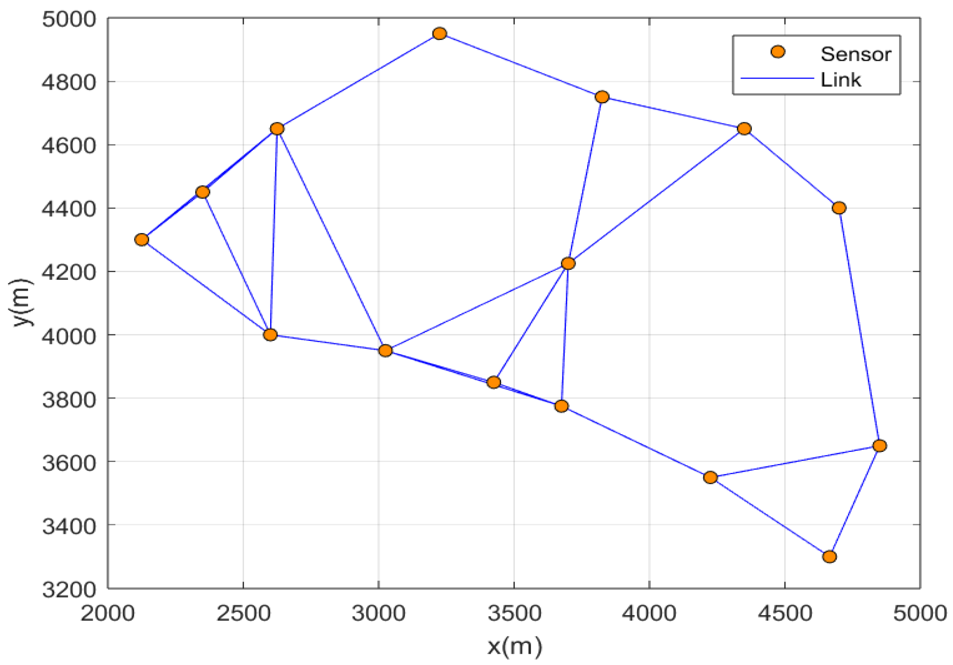
The measurement noise variance is $R=diag\left(\right[\begin{array}{cc}{15}^2& {15}^2\left]\right)\end{array}$ The sensor network comprises 15 nodes, and Figure 2 illustrates their network topology.

The initial state and covariance are

$$x_0={\left[\begin{array}{cccc}2600& 20& 3800& 10\end{array}\right]}^T$$

$$P_0=diag\left(\left[\begin{array}{cccc}{50}^2& 5^2& {50}^2& 5^2\end{array}\right]\right)$$

The process noise and measurement noise distributions with outliers is

$${\omega }_k\sim \left\{\begin{array}{c}N(0,Q)1-p_0\\ N(0,100Q)p_0\end{array}\right.$$

$$v_k^n\sim \left\{\begin{array}{c}N(0,R)1-p_0\\ N(0,100R)p_0\end{array}\right.$$

where $p_0$ is the probability of measuring outliers.

The remainder of this section is devoted to presenting the results of the simulation experiments. Three methods are compared: (1) Distributed Consensus Kalman Filter, named DCKF; (2) Distributed Consensus Student-t Filter, named DCSTF; (3) Distributed Consensus Kalman Filter with IMM, named DCKFIMM; and (4) the proposed algorithm, named DDMDFIMM.

The consensus iteration count for all of the above consensus filtering algorithms is 6, while the proposed algorithm just diffuses once.

Target maneuvers are simulated using a Markov chain model as follows:

$$\left\{\begin{array}{c}{F}_k=F_{k,2}or{F}_{k,3}ifrand>0.8;F_{k-1}=F_{k-1,1}\\ F_k=F_{k,1}or{F}_{k,3}ifrand>0.8;F_{k-1}=F_{k-1,2}\\ F_k=F_{k,1}or{F}_{k,2}ifrand>0.8;F_{k-1}=F_{k-1,3}\end{array}\right.$$

At each time step, the target’s motion model remains unchanged with a probability of 0.8. With a probability of 0.2, the model transitions to one of the two other models, each with a probability of 0.1. This results in a model transition probability matrix with dominant diagonal elements, reflecting the persistence of motion in real-world maneuvers.

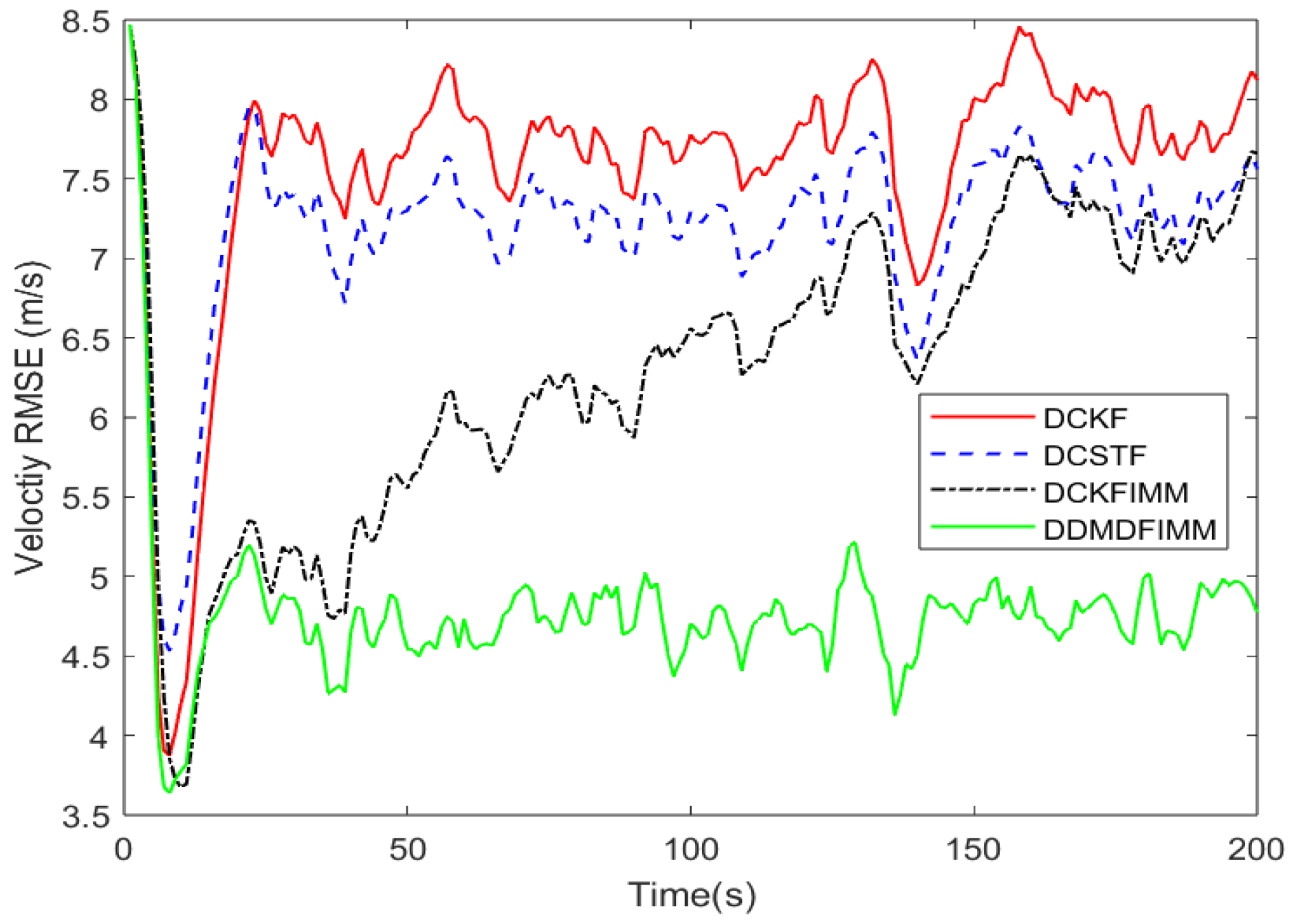
To evaluate performance in a Gaussian noise environment, the outlier occurrence probability $p_0$ was set to zero. Figure 3 illustrates the actual and estimated trajectories from a single simulation. Figure 4 and Figure 5 present the root mean squared error (RMSE) for position and velocity estimates generated by four algorithms. The DDMDFIMM algorithm demonstrates performance superior to other algorithms, while the DCKFIMM algorithm shows a considerably higher error. The DCSTF algorithm exhibits intermediate performance, while the DCKF shows considerably higher error. These findings indicate that, without outliers in maneuvering, Student-t models are more effective than Gaussian models, probably because Student-t treat dynamic measurement as outliers in the variance of motion mode. However, the DCKFIMM and DDMDFIMM algorithm, employing an IMM, achieves superior estimation accuracy; moreover, the DDMDFIMM employs an adaptive mixed model incorporating both Gaussian and Student-t distributions, showing better performance.

We assigned an outlier occurrence probability of $p_0$ = 0.2. The actual and estimated trajectories for a sample simulation are visualized in Figure 6. Figure 7 and Figure 8 depict the RMSE values for position and velocity, calculated for each of the three algorithms under consideration. As can be seen, the DCKF algorithm performed the worst. This is attributable to the inherent limitations of assuming a Gaussian distribution, which, while adequate for typical noise, proves inadequate when outliers are present. The DCKFIMM has a better performance than DCKF, and the performance of the DCKDIMM demonstrates performance comparable to the DCSTF algorithm probably because the present outlier degrades the performance of Gaussian distribution in the DCKFIMM algorithm. DDMDFIMM employs Student-t distribution, better reflecting the noise characteristics in the presence of outliers. Notably, DDMDFIMM achieved superior performance due to its hybrid distribution model, enabling adaptive model adjustments during estimation, thus enhancing robustness and accuracy.

This study employs a two-hypothesis model, incorporating both Gaussian and Student-t distributions, to address estimation in the presence of heavy-tailed noise. The selection of the Student-t distribution is motivated by its inherent flexibility, adjustable via its degrees of freedom, permitting approximation of both Gaussian and Cauchy distributions. State estimates obtained from both distributions are subsequently fused using a weighted average to achieve a balance between robustness and accuracy.

As can be seen from the

Table 1. Comparison without outliers.

	DCKF	DCSTF	DCKFIMM	DDMDFIMM
RMSE	27.0767	21.9831	21.2361	9.7129
TIME	0.3042	0.1466	0.5061	1.8484

and

Table 2. Comparison with outliers.

	DCKF	DCSTF	DCKFIMM	DDMDFIMM
RMSE	34.7188	17.7127	16.6515	12.1128
TIME	0.3031	0.1450	0.4971	1.8303

, although the method proposed in this paper performs well in terms of estimation accuracy, it has a relatively long running time. This is because it is the result of the joint application of IMM, hybrid noise distribution, and distributed networks, so this method is only suitable for situations with sufficient computing resources. In future research, we plan to use event-triggered methods to control the operation of IMM on nodes and the diffusion or consensus of distributed networks.

The communication overhead is a critical consideration in distributed state estimation, while the computational burden of multi-model algorithms is a direct consequence of the concurrent execution of multiple filtering processes, one for each model considered. Therefore, to reduce the computational cost, this algorithm uses diffusion instead of consensus with multi steps.

From the above simulation experiments, it can be seen that the method proposed in this paper is excellent in terms of estimation accuracy for maneuvering targets with outliers. In future practical deployment, it is first necessary to combine existing sensor hardware configurations, while using C language to optimize algorithms and data structures, and embed the algorithms into the hardware. Different modules must be mutually compatible, such as communication modules, signal transmission modules, and so on. Deploy the actual network using the overall principles of engineering theory. Before actual deployment, we will use semi-physical simulation to further verify the proposed method.

5. Conclusions

This paper presents a novel IMM distributed state estimation algorithm designed to handle heavy-tailed measurement noise in maneuvering target tracking. The proposed algorithm employs a multi-model, multi-distribution approach based on parallel Gaussian and Student-t filters. We successfully obtained a closed-loop solution for the hybrid noise distribution using the matrix matching method. The estimation accuracy is significantly better than that of a single noise distribution, both in the presence of obvious outlier noise and under normal conditions. We also used IMM to solve the problem of tracking maneuvering targets. It turned out that combining IMM with a hybrid noise distribution filter performed very well and was able to capture maneuvering targets effectively. The proposed diffusion algorithm exhibits good robustness when faced with different outliers in a single node. The method proposed in this paper provides inspiration for tracking and monitoring large radar networks, but specific deployment must still be considered in conjunction with various aspects (such as communications and hardware). However, the method proposed in this paper integrates algorithms from various fields, which results in a slightly cumbersome calculation process and a decrease in overall computing speed. This indicates that this method is only suitable for scenarios with sufficient computing resources and a focus on estimation accuracy and robustness. In the future, while further verifying this method, we plan to adopt an event-triggered approach to reduce the overall computing burden.

References

1. Bar-Shalom, Y. Multitarget Tracking: Applications and Advances; Artech House: Boston, MA, USA, 2000. [Google Scholar]
2. Reif, K.; Gunther, S.; Yaz, E.; Unbehauen, R. Stochastic stability of the discrete-time extended Kalman filter. IEEE Trans. Autom. Control. 1999, 44, 714–728. [Google Scholar] [CrossRef]
3. Julier, S.; Uhlmann, J.; Durrant-Whyte, H.F. A new method for the nonlinear transformation of means and covariances in filters and estimators. IEEE Trans. Autom. Control 2000, 45, 477–482. [Google Scholar] [CrossRef]
4. Shen, K.; Dong, P.; Jing, Z.; Leung, H. Consensus-Based Labeled Multi-Bernoulli Filter for Multitarget Tracking in Distributed Sensor Network. IEEE Trans. Cybern. 2022, 52, 12722–12733. [Google Scholar] [CrossRef]
5. Battistelli, G.; Chisci, L. Kullback–Leibler average, consensus on probability densities, and distributed state estimation with guaranteed stability. Automatica 2014, 50, 707–718. [Google Scholar] [CrossRef]
6. Cattivelli, F.S.; Sayed, A.H. Diffusion strategies for distributed Kalman filtering and smoothing. IEEE Trans. Autom. Control 2010, 55, 2069–2084. [Google Scholar] [CrossRef]
7. Hu, J.; Xie, L.; Zhang, C. Diffusion Kalman filtering based on covariance intersection. IEEE Trans. Signal Process. 2012, 60, 891–902. [Google Scholar] [CrossRef]
8. Li, X.R.; Jilkov, V. Survey of maneuvering target tracking. Part V: Multiple-model methods. IEEE Trans. Aerosp. Electron. Syst. 2005, 41, 1255–1320. [Google Scholar] [CrossRef]
9. Zhu, H.; Zhang, G.; Li, Y.; Leung, H. A novel robust Kalman filter with unknown non-stationary heavy-tailed noise. Automatica 2021, 127, 109511. [Google Scholar] [CrossRef]
10. Bishop, C.M. Recognition and Machine Learning (Information Science and Statistics); Springer: New York, NY, USA, 2006. [Google Scholar]
11. Arulampalam, M.; Maskell, S.; Gordon, N.; Clapp, T. A tutorial on particle filters for online nonlinear/non-Gaussian Bayesian tracking. IEEE Trans. Signal Process. 2002, 50, 174–188. [Google Scholar] [CrossRef]
12. Chen, B.; Liu, X.; Zhao, H.; Principe, J.C. Maximum correntropy Kalman filter. Automatica 2017, 76, 70–77. [Google Scholar] [CrossRef]
13. Ma, Y.; Zhao, S.; Huang, B. Multiple-Model State Estimation Based on Variational Bayesian Inference. IEEE Trans. Autom. Control 2019, 64, 1679–1685. [Google Scholar] [CrossRef]
14. Zhu, H.; Zhang, G.; Li, Y.; Leung, H. An Adaptive Kalman Filter With Inaccurate Noise Covariances in the Presence of Outliers. IEEE Trans. Autom. Control 2022, 67, 374–381. [Google Scholar] [CrossRef]
15. Huang, Y.; Zhang, Y.; Li, N.; Wu, Z.; Chambers, J.A. A Novel Robust Student’s t-Based Kalman Filter. IEEE Trans. Aerosp. Electron. Syst. 2017, 53, 1545–1554. [Google Scholar] [CrossRef]
16. Wang, G.; Yang, C.; Ma, X. A Novel Robust Nonlinear Kalman Filter Based on Multivariate Laplace Distribution. IEEE Trans. Circuits Syst. II Exp. Briefs. 2021, 68, 2705–2709. [Google Scholar] [CrossRef]
17. Huang, Y.; Zhang, Y.; Shi, P.; Chambers, J. Variational Adaptive Kalman Filter With Gaussian-Inverse-Wishart Mixture Distribution. IEEE Trans. Autom. Control 2021, 66, 1786–1793. [Google Scholar] [CrossRef]
18. Youn, W.; Huang, Y.; Myung, H. Outlier-Robust Student’s-t-Based IMM-VB Localization for Manned Aircraft Using TDOA Measurements. IEEE/ASME Trans. Mechatronics 2020, 25, 1646–1658. [Google Scholar] [CrossRef]
19. Xie, G.; Sun, L.; Wen, T.; Hei, X.; Qian, F. Adaptive Transition Probability Matrix-Based Parallel IMM Algorithm. IEEE Trans. Syst. Man Cybern. Syst. 2021, 51, 2980–2989. [Google Scholar] [CrossRef]
20. Wang, G.; Wang, X.; Zhang, Y. Variational Bayesian IMM-Filter for JMSs With Unknown Noise Covariances. IEEE Trans. Aerosp. Electron. Syst. 2020, 56, 1652–1661. [Google Scholar] [CrossRef]
21. Youn, W.; Huang, Y.; Myung, H. Robust Localization Using IMM Filter Based on Skew Gaussian-Gamma Mixture Distribution in Mixed LOS/NLOS Condition. IEEE Trans. Instrum. Meas. 2020, 69, 5166–5182. [Google Scholar] [CrossRef]
22. Blom, H.; Bar-Shalom, Y. The interacting multiple model algorithm with Markovian switching coefficients. IEEE. Trans. Autom. Control 1988, AC-33, 780–783. [Google Scholar] [CrossRef]
23. Hwang, I.; Seah, C.E.; Lee, S. A Study on Stability of the Interacting Multiple Model Algorithm. IEEE Trans. Autom. Control 2017, 62, 901–906. [Google Scholar] [CrossRef]
24. Cui, T.; Jing, Z.; Dong, P. Variational Bayesian Multiple Model Filter in the Presence of Outliers. IEEE Sens. J. 2024, 24, 12985–12994. [Google Scholar] [CrossRef]
25. Huang, Y.; Zhang, Y.; Zhao, Y.; Chambers, J.A. A novel robust Gaussian-student’s T mixture distribution based Kalman filter. IEEE Trans. Signal Process. 2019, 67, 3606–3620. [Google Scholar] [CrossRef]
26. Bruno, M.; Dias, S. A Bayesian interpretation of distributed diffusion filtering algorithms [Lecture Notes]. IEEE Signal Process. Mag. 2018, 35, 118–123. [Google Scholar] [CrossRef]
27. Chang, G.; Fu, W.; Song, L.; Cui, T.; Dong, P. Distributed Consensus Multi-Distribution Filter for Heavy-Tailed Noise. J. Sens. Actuator Netw. 2024, 13, 38. [Google Scholar] [CrossRef]
28. Hage, J.; Xu, P.; Bonnifait, P. Student’s t information filter with adaptive degree of freedom for multi-sensor fusion. In Proceedings of the 2019 22th International Conference on Information Fusion (FUSION), Ottawa, ON, Canada, 2–5 July 2019; IEEE: New York, YK, USA, 2019. [Google Scholar]
Figure 1. Architectural diagram of DDMDIMM filter.
Signals 06 00037 g001
Figure 2. Topology of sensor network.
Signals 06 00037 g002
Figure 3. The true and estimated trajectories.
Signals 06 00037 g003
Figure 4. Position root mean square errors of different algorithms.
Signals 06 00037 g004
Figure 5. Velocity root mean square errors of different algorithms.
Signals 06 00037 g005
Figure 6. The true and estimated trajectories.
Signals 06 00037 g006
Figure 7. Position root mean square errors of different algorithms.
Signals 06 00037 g007
Figure 8. Velocity root mean square errors of different algorithms.
Signals 06 00037 g008