Improved RSSI Indoor Localization in IoT Systems with Machine Learning Algorithms

Abstract

Recent developments in machine learning algorithms are playing a significant role in wireless communication and Internet of Things (IoT) systems. Location-based Internet of Things services (LBIoTS) are considered one of the primary applications among those IoT applications. The key information involved in LBIoTS is finding an object’s geographical location. The Global Positioning System (GPS) technique does not perform better in indoor environments due to multipath. Numerous methods have been investigated for indoor localization scenarios. However, the precise location estimation of a moving object in such an application is challenging due to the high signal fluctuations. Therefore, this paper presents machine learning algorithms to estimate the object’s location based on the Received Signal Strength Indicator (RSSI) values collected through Bluetooth low-energy (BLE)-based nodes. In this experiment, we utilize a publicly available RSSI dataset. The RSSI data are collected from different BLE ibeacon nodes installed in a complex indoor environment with labels. Then, the RSSI data are linearized using the weighted least-squares method and filtered using moving average filters. Moreover, machine learning algorithms are used for training and testing the dataset to estimate the precise location of the objects. All the proposed algorithms were tested and evaluated under their different hyperparameters. The tested models provided approximately 85% accuracy for KNN, 84% for SVM and 76% accuracy in FFNN.

1. Introduction

With the rapid development of IoT- and AI-integrated technologies, researchers and developers have been driven to create intelligent location-based IoT applications for smart cities, transportation, intelligent buildings, smart agriculture, military applications, etc. Location-based services (LBS) are among these applications, and they are regarded as crucial ones since LBS makes it possible to determine the precise location of moving objects in enclosed spaces. Many people spend a day in indoor environments because of work, school, shopping, etc. Therefore, LBIoTSs play a significant role in this era by locating objects in indoor environments and providing crucial information for many intelligent applications, for example, locating an older person who is living alone in a house, locating a human in a shopping mall, automatically taking students’ attendance on a smart campus, locating a person using a wearable sensor in a hospital, locating people inside a building during a fire, etc. [1,2].

Regarding localization, there are two environments: outdoor and indoor. GPS technology is well performed in outdoor environments; however, it is inappropriate for indoor localization due to several reasons [3,4]. The GPS will not work accurately in the indoor environment due to the multipath fading effect and less accuracy in estimation [5]. Due to the above reasons, researchers have developed indoor localization algorithms based on deterministic algorithms, probabilistic algorithms, and filters. Many widely used deterministic and probabilistic algorithms can be found in related works, such as trilateration, multilateration, the Levenberg–Marquardt algorithm, and Kalman filters [6]. The drawbacks of the mentioned algorithms are lower accuracy, inefficiency, complex hardware systems, and most of the time, they are impractical to deploy in robust indoor environments.

Similar works exist on using ML techniques for indoor localization applications. The existing works can be categorized as supervised regressor-based, classifier-based, deep learning-based, and unsupervised learning-based approaches. The works [7] used a supervised regressor to find the location. In contrast, different types of regressors, such as Decision Tree Regression, Random Forest Regression, Linear Regression, Polynomial Regression, Support Vector Regression, and Extra Tree Regression, have been employed. The results indicate that RFR, SVR, and ETR perform better than other algorithms. While various ML-based frameworks have been proposed, certain algorithms need to be carefully analyzed, taking into consideration the practicality of implementing them on real hardware devices. There is a high impact of RSSI data filtering on localization accuracy. In the literature, many works have proposed linear and non-linear filters to filter the collected data. The works [8,9] used moving average filters, and [10,11] used Kalman and extended Kalman filters when smoothing RSSI data. Though Kalman filters outperform moving average filters, the moving average filters are widely used due to their simplicity [12].

The works [12,13,14,15,16] have used supervised classifiers for indoor localization. Neural Networks (NN), Feed Forward Neural Networks (FFNNs), SVM, and kNN are used as ML algorithms. According to [16], NN is good in accuracy, but it requires high computational power. The kNN also gives a reasonable accuracy. MATLAB, a Python-based IDE, has been used to implement these algorithms. During the evaluation of performances, confusion matrices are used. One crucial observation is that a standard ML algorithm cannot be proposed for all indoor applications because the outperformed algorithm varies due to many reasons, such as wireless technology, signal measurement techniques, the types of filters used, the environment’s robustness, the computational power of devices, the dataset’s size, the dataset’s hyperparameter tuning aspects, etc.

This paper investigates how to use supervised classifiers for indoor localization, where locations are estimated as categorical data with improved RSSI linearization. We introduced a novel linearization and filtering mechanism with ML framework to improve the localization accuracy in robust indoor localization systems. For this experiment, we used a publicly available testbed and its dataset [17]. In this case, we consider the location estimation as a classification-type ML problem, and where the specific location (zone) of an existing person will be predicted. This testbed consists of 13 BLE ibeacon nodes implemented inside a library. In addition, high security, a low cost, and minimal power consumption are all benefits of Bluetooth positioning technology; yet, Bluetooth has poor signal reliability and a limited communication range. More details on the dataset and testbed will be discussed later in this paper. We used the RSSI dataset for pre-processing using a moving average filter and weighted least-squares method. Afterward, the dataset was trained by the supervised classifiers FFNN, SVM, and kNN, and we evaluated each algorithm’s performance on localization. However, this study was limited to one particular BLE dataset, and other wireless technologies were not considered.

This paper is organized as follows: firstly, the background theory of wireless indoor localization will be discussed in the background section. Secondly, related works in ML for indoor localization and the mathematical model will be discussed. Thirdly, our novel system model is proposed. In the fourth section, we elaborate on the steps of data pre-processing and the ML-model development and training. The fifth section discusses the model evaluation in detail, including the hyperparameter tuning for each model. Finally, we conclude the findings.

Wireless indoor localization is a technique that estimates the objects’ location by using distance measurements. Primarily, indoor localization systems can be categorized as device-free and device-based localization. Typically, these location localization techniques require distance measurements as input for the algorithm. The widely used distance measurement techniques in positioning systems are the Angle of Arrival (AoA), Time of Arrival (ToA), Time of Flight (ToF), Time Difference of Arrival (TDoA), Channel State Information (CSI), and Received Signal Strength Indicator (RSSI). When comparing the above distance measurement techniques, there are pros and cons. For instance, the AoA system uses a set of antennae to determine the signal propagation angle, since more hardware is needed and implementation cost is high. The AoA technology typically requires complex hardware such as antenna arrays calibrated to get the correct position. The RSSI level correlates the distance between the transmitter and the receiver. Additionally, the signal intensity weakens as it goes away from the transmitter; it is frequently used to calculate the separation between a transmitter and the receiver of the nodes. Because the transmitting signal is vulnerable to environmental noise and multipath fading, RSSIs generally lead to inaccurate values and errors in localization systems; therefore, strong signal processing techniques should apply before it is processed through ML algorithms. Once it has a distance measure, it can feed as the input for the algorithm. Before being fed into the algorithms, it requires strong signal filtering. Specific algorithms require a bare minimum number of anchor nodes. For instance, trilateration requires at least three anchor nodes in the system [17,18,19].

2. Related Works

This section provides an overview of related studies carried out on Indoor Localization estimation techniques with different machine-learning algorithms.

Aigerim et al. employed an ML classifier-based approach for indoor localization. The experiment tested the RSSI data collected from mobile devices (Sony Xperia XA1) and BLE product iTAG sent-out signals. The location column showed the iTAG at the building’s entrance. Students assisted in the collection of the dataset. Three groups of twelve students each had an iTAG device formed. They entered the constrained space with their iTAGs turned on. Three marked locations represented the building’s entrance—inside, in the vestibule, and outside—on an 18.35 m × 3 m long hallway. Signals were collected using two Sony Xperia XA1 smartphones, which were located at the beginning and end of the 2.35 m long “in vestibule” space. The collection of RSSIs lasted for twenty minutes. The raw RSSIs and filtered RSSIs were the two datasets. Actual RSSIs from a smartphone are known as raw RSSIs. To smooth RSSIs, a feedback filter is used. The filtered data were trained using Naive Bayes and Support Vector Machine algorithms, and their results showed 0.95 accuracy for SVM when it had four vectors.

Singh et al. contributed to investigating mobile phone-based indoor localization using ML techniques. They set up an indoor experimental testbed, gathered 3110 RSSI data points, and assessed the effectiveness of many machine learning methods. The algorithm was tested with kNN, RFR, Multilayer and Perceptron, and ZeroR. It was concluded that the proposed methods surpassed other indoor localization methods, with a mean error as exact as 0.76 m. The study also suggested a hybrid instance-based strategy that, compared to conventional instance-based methods, accelerates performance by a factor of ten without sacrificing accuracy. Furthermore, the proposed study was examined on its precision, crucial usage in real-world settings, and how it was affected by less-dense datasets. Finally, by analyzing their performance in an online, in-motion experiment, they showed that these techniques are suitable for real-world deployment [20].

Kaur et al. investigated RSSI- and ML-based approaches for indoor localization. In this study, the researchers used Neural Networks to carry out localization strategies based on the RSSI measurements. The RSSI dataset was collected from the experiment in [14], and the position estimate outcomes were compared with two approaches (the ANN and the Decision Tree). The proposed study first employed an Artificial Neural Network with three inputs to estimate the position of each RSSI’s triplet. Then, it calculated the mean’s error value for each position acquired. A similar process was performed for the ANN design with four inputs, where they estimated the position for each of the four inputs and determined the mean’s error value for these estimates. In summary, the tested algorithms achieved better precision than the Decision Tree algorithm [21].

Jun et al. contributed by applying a weighted least-squares Techniques to RSSI-based localization to improve its accuracy. The study employed a weighted multilateration approach to make it more resilient to errors and less dependent on an ideal channel model. Two weighted least-squares techniques based on the conventional hyperbolic and circular positioning algorithms were used to estimate the precise location. These methods specifically took the accuracy of the various data into account. Through extensive real-world testing on different wireless network types and numerical simulations, these methodologies were contrasted against the conventional hyperbolic and circular positioning methods (a wireless sensor network, a Wi-Fi network, and a Bluetooth network). The methods yielded an increased tolerance to environmental changes as well as improved localization results, with very little additional processing expense [14].

Xudong et al. proposed a deep learning-based method for indoor localization in multi-floor environments. In this research work, they presented an improved algorithm based on deep learning, namely CNNLoc, a Convolutional Neural Network (CNN)-based indoor localization system with WiFi fingerprints for multi-story buildings and multi-floor localization. The authors contributed explicitly towards creating a novel classification model by fusing a one-dimensional CNN and a stacked auto-encoder (SAE). While the CNN was trained to attain high accuracy rates in the positioning phase efficiently, the SAE was used to precisely extract critical characteristics from sparse Received Signal Strength (RSS) data. Further, they assessed the proposed system using several cutting-edge techniques on the UJIIndoorLoc and Tampere datasets. The findings demonstrated that the CNNLoc outperformed the existing methods, with success rates of 100% for building-level localization and also 95% for floor-level localization, respectively, where the results showed very high accuracy. Further, in [22], a framework for indoor localization with NN based on smartphones was proposed. Table 1 shows the comparison study of the existing works and finding.

Table 1. Comparison study of the existing works and to finding.

Proposed Methodologies for Localization	Machine Learning Algorithms Used	The Complexity of the Algorithm	Remarks
Localization of nodes [14]	Convolutional Neural Networks	Moderate	Giving good accuracy; signal filtering and linearization not investigated
Human Localization [15]	Neural Networks	Moderate	77% accuracy, no comparison with other algorithms
Localization based on NNs [16]	Neural Networks	High	78% accuracy, only NN was investigated and no comparison with other types of ML techniques
Localization using SVM [17]	Support Vector Machine	Moderate	82% accuracy, high power consumption as Wi-Fi was used
Underwater Surveillance System [18]	Decision Tree-Based Localization	Low	Decent accuracy of DT, no hyperparameter tuning for DT algorithm
Distributed Localization [19]	Self-Organizing Map	Moderate	Fairly good accuracy provided. Wi-Fi was used
Soft Localization [20]	Neural Networks	Moderate	Providing a low accuracy. No comparison with other ML models. None of the linearization techniques were investigated.

All the above works provided the potential to use ML techniques in the localization problem. Yet, the comparative analysis of the performance of multiple algorithms, linearization of RSSI signals, and hyperparameter tuning was lacking in the present works. Further, the performance of the model also highly depends on the dataset, wireless technology used, filter techniques, and linearization used. Advanced ML techniques, such as Deep Learning, require a large dataset for more accurate results. Additionally, the nature of the dataset causes overfitting and underfitting in ML models.

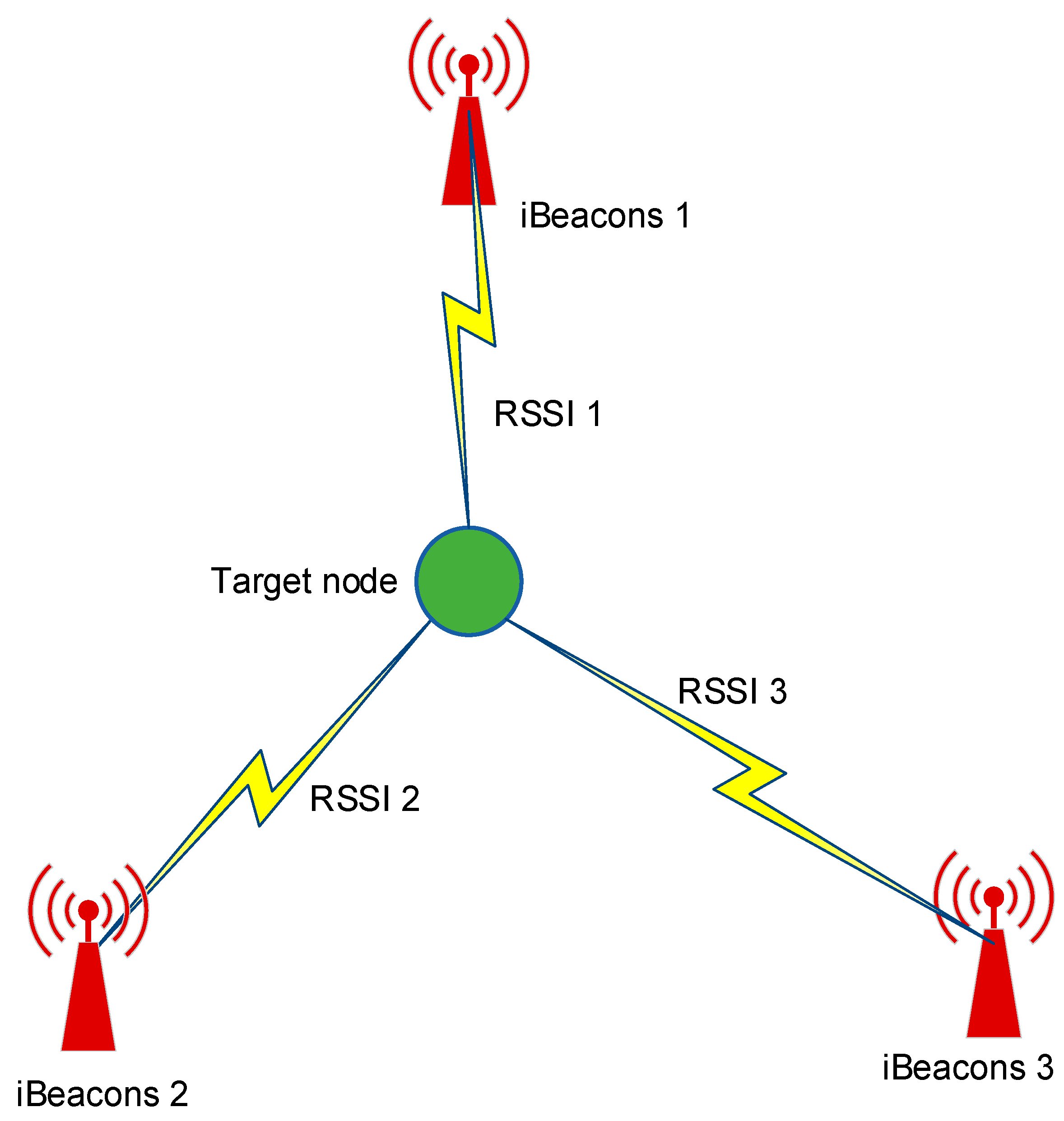
Received Signal Strength Indicator

The Received Signal Strength Indicators (RSSI) is a well-known location estimation approach, in which the power-intensity value is assessed from the beacons and measured in dBm. The RSSI measurements for one particular location of the target node are collected, as shown in Figure 1.

Figure 1. Arrangement of anchor node and target nodes.

The RSSI value defines the distance between beacons and the target node, and the value increases accordingly as the distance increases. The logarithmic distance loss model is calculated as Equation (1) [5]:

$$RSS{I}_r(p)=RSS{I}_r(p_0)-10\eta \log \frac{p}{p_0}+X_{\sigma }$$

(1)

where $RSS{I}_r(p)$ is defined as the received power [dBm] at a distance $p$ [m] from the transmitter, $X_{\sigma }$ is defined as a zero-mean Gaussian random variable with the variance of $\left(\mathbb{N}(0,{\sigma }^2)\right)$, $RSS{I}_r(p_0)$ refers to the received power [dBm] at the reference distance $p_0$ from the transmitter, and $\eta$ is the path loss exponent, which varies from 2 in free space to 4 in indoor environments. The localization algorithm is applied to estimate the location of the target node with the distances to different beacons. In this study, we proposed a weighted least-squares method for improved RSSI-based localization. The basic idea of the proposed algorithm was to find the position $\left(a,b\right)$ of the target node that decreased the sum of the squared error values. Let $p_n=(a_n,b_n)$ be the location of beacons, such that $n (n=1, 2, \dots , N$), where $N$ is the total number of beacons and ${\tilde{p}}_n$ is the estimated location of the beacons. Therefore, the square of the distance between the target node and the beacon node $n$ is calculated as

$$p_n^2={(a_n-a)}^2+{(b_n-b)}^2$$

(2)

The starting point is used at the beacon $n=1$, such that, $a_1=b_1=0$. Therefore, for $n>1$,

$$p_n^2-p_1^2=a_n^2-2a{a}_n+b_n^2-2b{b}_n$$

(3)

Therefore, Equation (3) can be written in Matrix as

$$\left[\begin{array}{ccc}2a_2& & 2b_2\\ ⋮& & ⋮\\ 2a_N& & 2b_N\end{array}\right]\left[\begin{array}{c}a\\ b\end{array}\right]=\left[\begin{array}{c}{a}_2^2+b_2^2-p_2^2+p_1^2\\ ⋮\\ a_N^2+b_N^2-p_N^2+p_1^2\end{array}\right]$$

(4)

The above, Equation (4), can be written as

$$M·\tilde{A}=\tilde{C}$$

(5)

where $M=\left[\begin{array}{ccc}2a_2& & 2b_2\\ ⋮& & ⋮\\ 2a_N& & 2b_N\end{array}\right],\tilde{A}=\left[\begin{array}{c}a\\ b\end{array}\right]$ and $\tilde{C}$ defines the random vector as

$$\tilde{C}=\left[\begin{array}{c}{a}_2^2+b_2^2-p_2^2+p_1^2\\ ⋮\\ a_N^2+b_N^2-p_N^2+p_1^2\end{array}\right]$$

(6)

Thus, the location of the target node is estimated by using the linear least-square method as

$$\tilde{A}={(M^{T}M)}^{-1}{M}^T\tilde{C}$$

(7)

The localization is dependent on ${(M^{T}M)}^{-1}$. The expression $M^{T}M$ is a square, non-singular, and invertible matrix if the beacons are reasonably far from the target node.

We applied weighted least-squares in Equation (5) as

$$\tilde{A}={(M^T{R}^{-1}M)}^{-1}{M}^T{R}^{-1}\tilde{C}$$

(8)

where R defines the covariance matrix of the vector $\tilde{C}$ and is written as

$$R=\left[\begin{array}{cccc}Var({\tilde{p}}_1^2)+Var({\tilde{p}}_2^2)& Var({\tilde{p}}_1^2)& \dots & Var({\tilde{p}}_1^2)\\ Var({\tilde{p}}_1^2)& Var({\tilde{p}}_1^2)+Var({\tilde{p}}_3^2)& \dots & Var({\tilde{p}}_1^2)\\ ⋮& ⋮& \ddots & \\ Var({\tilde{p}}_1^2)& Var({\tilde{p}}_1^2)& \dots & Var({\tilde{p}}_1^2)+Var({\tilde{p}}_N^2)\end{array}\right]$$

(9)

Therefore, the value of the covariance matrix R is evaluated as

$$Var ({\tilde{p}}_n^2)=E\left[{\tilde{p}}_n^4\right]-{\left(E\left[{\tilde{p}}_n^2\right]\right)}^2$$

(10)

Now, by using the channel condition model, the estimated location ${\tilde{p}}_n$ of Equation (1) is

$${\tilde{p}}_n=p_n·{10}^{\frac{N(0,\sigma )}{10\eta }}={10}^{N\left(\log 10p_n,\frac{\sigma }{10\eta }\right)}=e^{N\left(\log 10p_n,\frac{\sigma }{10\eta }\right)}=e^{N\left(\ln p_n,\frac{\sigma \ln 10}{10\eta }\right)}$$

(11)

where ${\tilde{p}}_n$ defines the lognormal random variable, along with parameters ${\sigma }_p=\ln p_n$ and ${\sigma }_p=\frac{\sigma \ln 10}{10\eta }$. The jth moment of a lognormal random variable of parameters $({\mu }_p,{\sigma }_p)$ is given by ${\mu }_j=e^{j·{\mu }_p+\frac{1j_{}^2{\sigma }_p^2}{2}}$.

Therefore,

$$E\left[{\tilde{p}}_n^4\right]=\exp \left(4{\mu }_p+8{\sigma }_p^2\right)$$

(12)

$$E\left[{\tilde{p}}_n^2\right]=\exp \left(2{\mu }_p+2{\sigma }_p^2\right)$$

(13)

Then, we put Equations (12) and (13) in Equation (10) as

$$Var ({\tilde{p}}_n^2)=E\left[{\tilde{p}}_n^4\right]-{\left(E\left[{\tilde{p}}_n^2\right]\right)}^2=\exp \left(4{\mu }_p\right)·\left(\exp \left(8{\sigma }_p^2\right)-\exp \left(4{\sigma }_p^2\right)\right)$$

(14)

Here, ${\mu }_p$ is dependent on the actual location $p_n$ and estimation location ${\tilde{p}}_n$ of the target node and the iBeacons. Therefore, the proposed weighted least-squares method solves the non-linear problem of RSSI-based localization and provides a precise estimation of the target location.

3. System Model

3.1. Machine Learning for Wireless Indoor Localization

Machine learning algorithms can be categorized into supervised, semi-supervised, and unsupervised learning algorithms. The supervised learning algorithms required a labeled dataset for predictions, and unsupervised algorithms used an unlabeled dataset for their predictions. The typical ML lifecycle has several stages: data pre-processing, model training, hyperparameter tuning, and model evaluation. ML algorithms can be used for classification or regression tasks. In classification, machine learning algorithms classify data into different categories, while regression learns from training data to predict continuous variables. The object’s location can be estimated as a numerical value (regression) or as a classification (classifiers). For example, consider a person living inside a house and obtaining the location through an IoT system. The location of the person or object can be estimated geographically with coordinates or can predict the location as an area such as the bedroom, kitchen, etc. In this work, we have selected three algorithms, and each algorithm’s brief details are given as follows.

3.1.1. Artificial Neural Networks

Artificial Neural Networks considers a powerful ML technique that can be applied to indoor localization systems. The basic working of an ANN is like the human neural network in our brain. The ANN follows the same structure of how brain neurons are interconnected. The ANN has three layers: the input layer, the hidden layer(s), and the output layer. The ANN has many advantages. Once the ANN is trained, the model will provide the output even with inadequate data. Moreover, ANN has a memory distribution, manages fault tolerance, and has a flexible network structure. The ANN performance is highly dependent on the hardware it runs.

A Feed-Forward Neural Network (FFNN) is considered a sub-branch of ANN. An FFNN consists of at least one layer of neurons and input and output layers. The network’s intensity can be observed based on the collective behavior of the connected neurons. The output is chosen by evaluating the network’s output in its input context. The main benefit of this network is that it learns to assess and identify input patterns. Generally speaking, an Artificial Neural Network has three layers, named the input layer, the hidden layer, and the output layer. Few works in the literature have used FFNN for indoor localization, giving considerably good results. However, it was observed that ANNs require a considerable computational time and capacity.

3.1.2. Support Vector Machine

The SVM is a machine learning algorithm that uses labeled training samples to learn the classification of data points. For example, one way to detect malicious behavior on a node is to use SVMs to investigate the temporal and spatial correlation of data. To explain this point, the WSN observation is used as a point in the element space, and the SVM divides it into multiple parts. These parts are separated by the widest possible margin (the separation gap), and the new readings are sorted according to which side of the gap they are on. An SVM algorithm uses linear constraints to optimize a quadratic function (the problem of building a set of hyperplanes). It provides an alternative to Multi-layer Neural Networks with non-convex, unconstrained optimization problems.

3.1.3. K-Nearest Neighbor Algorithm

K-Nearest Neighbor (kNN) is considered the simplest classifier used for indoor positioning systems. The kNN algorithm uses a feature-similarity approach for prediction. The kNN algorithm can be used for both classification- and regression-type problems. In this study, the nearest neighbors were those data points with a minimal distance in the feature space from the new data point. Additionally, the value k was the number of such data points we considered in implementing the algorithm. For example, a number k was selected by KNN algorithms as the nearest neighbor to the data point that needed to be categorized. For instance, if k is 3, it will search for the three closest neighbors to that data point, where k is the hyperparameter of the kNN algorithm. The value of k has an impact on the model accuracy. A prepared table that lists the relative strengths of two or more separate received signals from neighborhood routers is necessary for the kNN algorithm. The offline phase is when the predetermined table is built.

3.2. Testbed and Dataset

We used the publicly available dataset in [23] for our experiments. The dataset used in this experiment is available [8]. In this experimental setup, the dataset seen in Figure 2 was created using the RSSI readings from a set of 13 iBeacons on the first floor of the Waldo Library at Western Michigan University. The data were collected using an iPhone 6S, Apple USA. A labeled dataset (1420 samples) and an unlabeled dataset (1420 samples) were included in the dataset (5191 samples). In the original dataset in [8] authors have numbered the experiment area from A to U as rows and 1–18 as columns. In the experiment each cell has a unique identification number i.e B3001 as in Figure 2. When it comes to our experiment, the total experiment area divided in to four zones as A, B, C and D for simplicity and the ML models developed to estimate the location as one of these zones as a categorical problem. The recording was completed within the library’s regular operating hours. During the experiments, other wireless devices were switched off to reduce the disturbances from the different sources. More significant RSSI values showed a nearer proximity to a given iBeacon. For out-of-range iBeacons, the RSSI was shown by −200. Figure 2 shows the layout of the plan of iBeacons in green color circles. For the experimentation, we used only the labeled dataset given by the authors.

Figure 2. Arrangement of the sensor nodes in the testbed [8].

4. Model Training and Evaluation

In this work, we followed the machine learning life cycle to develop the models for location estimation. We started with data pre-processing, where row RSSI data were linearized and filtered. Additionally, we trained our models with the row RSSI dataset to understand the proposed filtering effect in location estimation accuracy. Then, the dataset was trained using ML models implemented using the scikit-learn ML library available in Python 3. All the models were developed on a Jupyter Notebook. Each stage of the implementation is explained as follows.

4.1. Data Pre-Processing

The RSSI dataset consisted of 5191 data and was filtered using the moving average filters. The moving average (MA) filter is the most common and widely used filter in digital signal processing because it is the most accessible digital filter in this kind of application. The row RSSI data in both the time and frequency domains are shown in Figure 3. Where we have only plotted the RSSI data received from three access points to understand the fluctuation and nature of the signals. The RSSI values received from access points one, two and three are shown in black, orange and blue color in the Figure 3.

Figure 3. RSSI data with frequency and time domain.

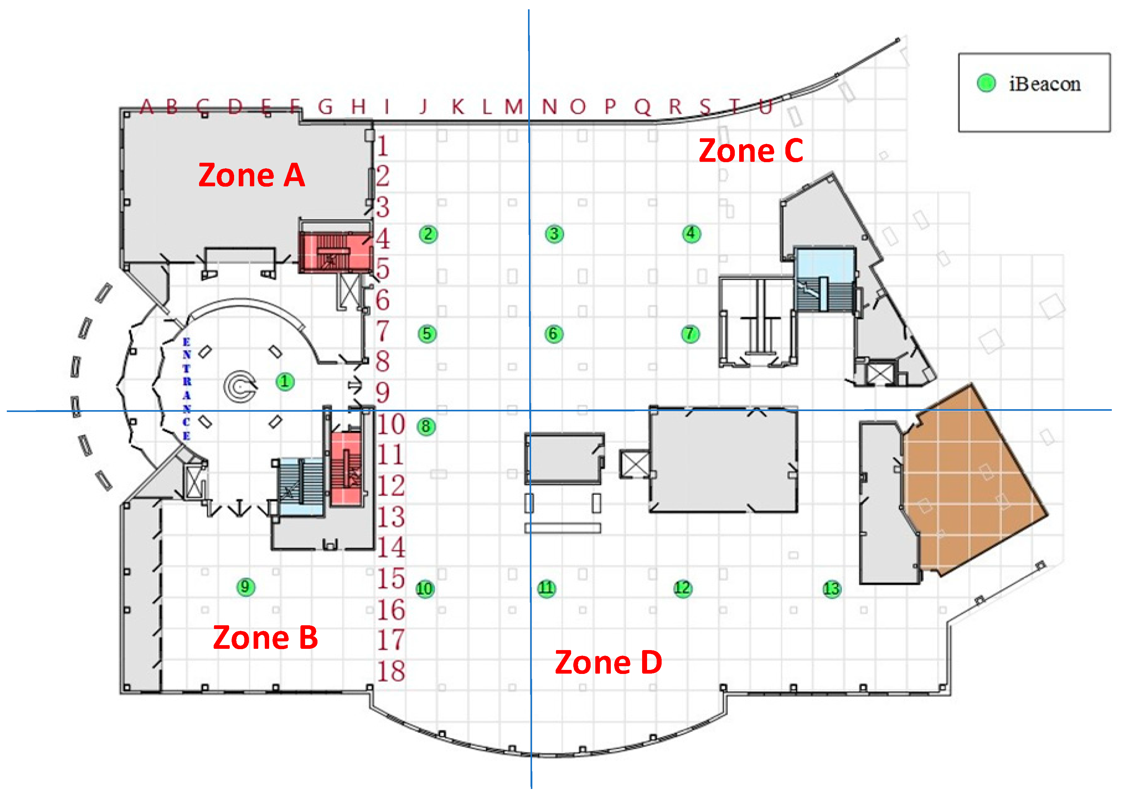
After the filtering, four columns were added to the dataset, as shown in Table 2, where zones A, B, C, and D were shown as per Figure 2. This modification was performed as we needed to train our ML models as a classification task. Table 2 shows the original dataset, where the location column denotes the location ID allocated for each location, and OO2, PO1, PO2 and PO3 are the RSSI levels received by the anchor nodes. Table 3 shows the dataset modified for classification purposes, where four new columns are added.

Table 2. A few data samples from the original dataset.

Location	OO2	PO1	PO2	PO3
B3001	−200	−200	−200	−200
B3002	−200	−200	−200	−200
B3003	−200	−200	−200	−200
B3004	−200	−200	−200	−200
B3005	−200	−200	−200	−200
B3006	78	−78	−77	−77
B3007	−200	−200	−200	−200
B3008	−200	−200	−200	−200
B3009	−200	−200	−200	−200
B3010	−200	−200	−200	−200
B3011	−200	−200	−200	−200
B3012	−200	−200	−200	−200
B3013	−200	−200	−200	−200

Table 3. A few samples from the modified dataset.

Location	OO2	PO1	PO1	PO1
B3001	−200	−200	−200	−200
B3002	−200	−200	−200	−200
B3003	−200	−200	−200	−200
B3004	−200	−200	−200	−200
B3005	−200	−200	−200	−200
B3006	−78	−78	−77	−77
B3007	−200	−200	−200	−200
B3008	−200	−200	−200	−200
B3009	−200	−200	−200	−200
B3010	−200	−200	−200	−200
B3011	−200	−200	−200	−200
B3012	−200	−200	−200	−200
B3013	−200	−200	−200	−200
Zone A	0	0	0	0
Zone B	0	0	0	0
Zone C	1	1	1	1
Zone D	0	0	0	0

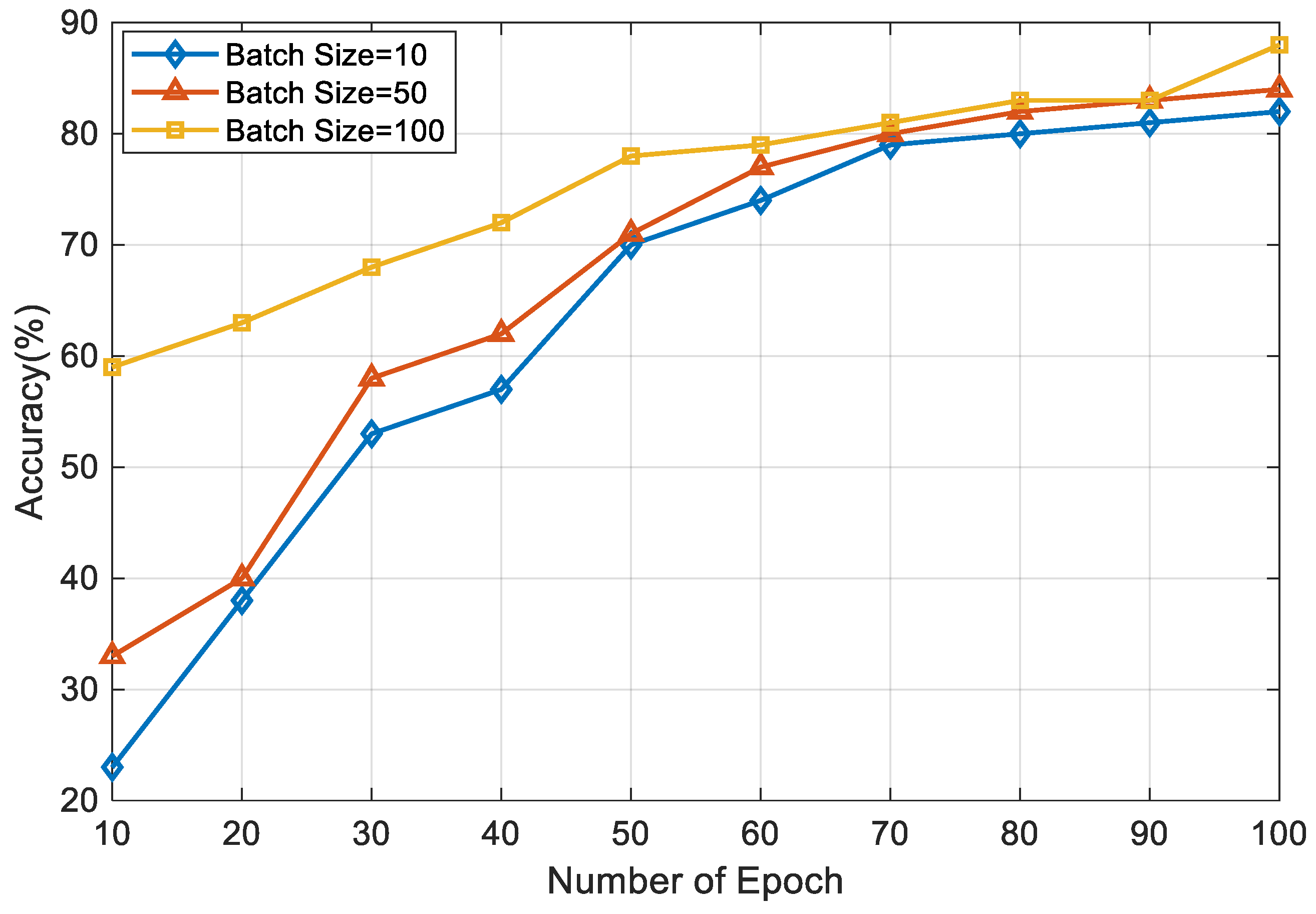
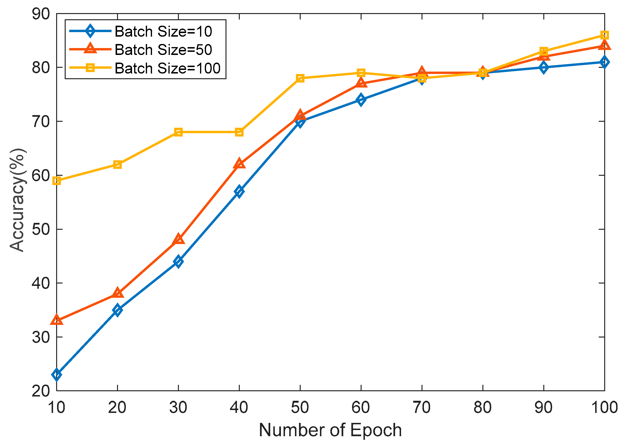
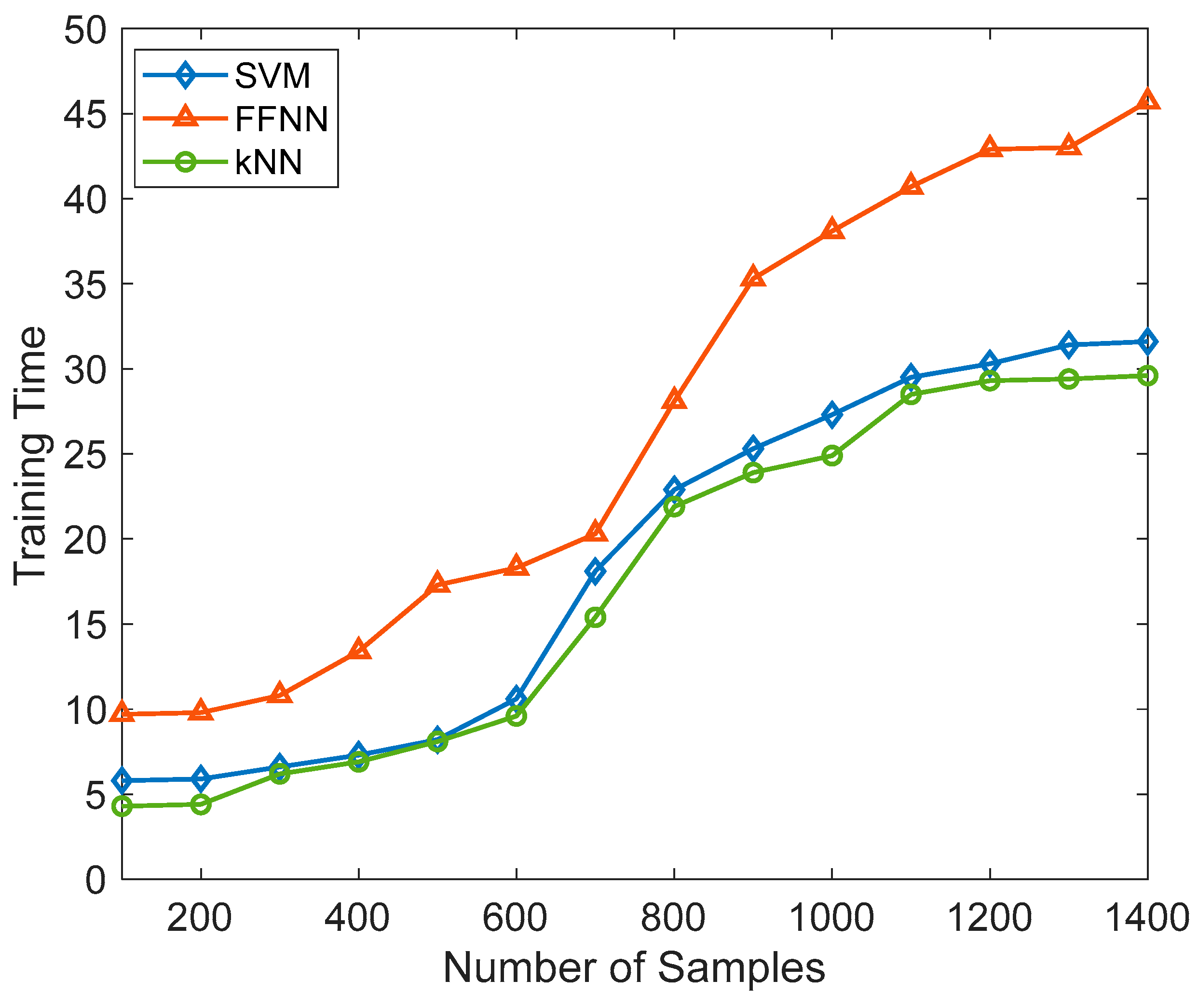
4.2. Model Training

The filtered RSSI dataset was trained using FFNN, SVM, and kNN, respectively. The proposed FFNN architecture comprised two fully connected layers and one output layer, as shown in Figure 4. This FFNN had three layers, where, thirteen inputs were presented at the input layer as it had thirteen beacon node inputs. And it had one hidden layer and the output layer. The first fully connected layer included twenty neurons, while the second fully connected layer had seventeen neurons. For all simulations, the network architecture had four completely linked levels and one categorization layer. Using the neural network toolkit in MATLAB 2020, the FFNN was implemented. Moreover, the FFNN was trained underneath three different hyper-parameters values of the learning rate (LR), batch size, and epochs. The activation function of the FFNN is very important as it is accountable for transforming the node’s summed weighted input into the node’s activation. Here, we used the ReLU activation function, which will output the input directly if it is positive; otherwise, it is zero. Moreover, ReLU is easy to train and provides better performance. To increase the model’s accuracy during the simulations, the ReLU activation function in fully connected layers and the SoftMax function in the final layer were both utilized. We re-trained our model data-interpolating techniques to generate new samples between existing data points. This did not increase the accuracy significantly, but we observed smoother representation of the signal variations. This information is mentioned in the manuscript.

Figure 4. Testing accuracy vs. number of epochs.

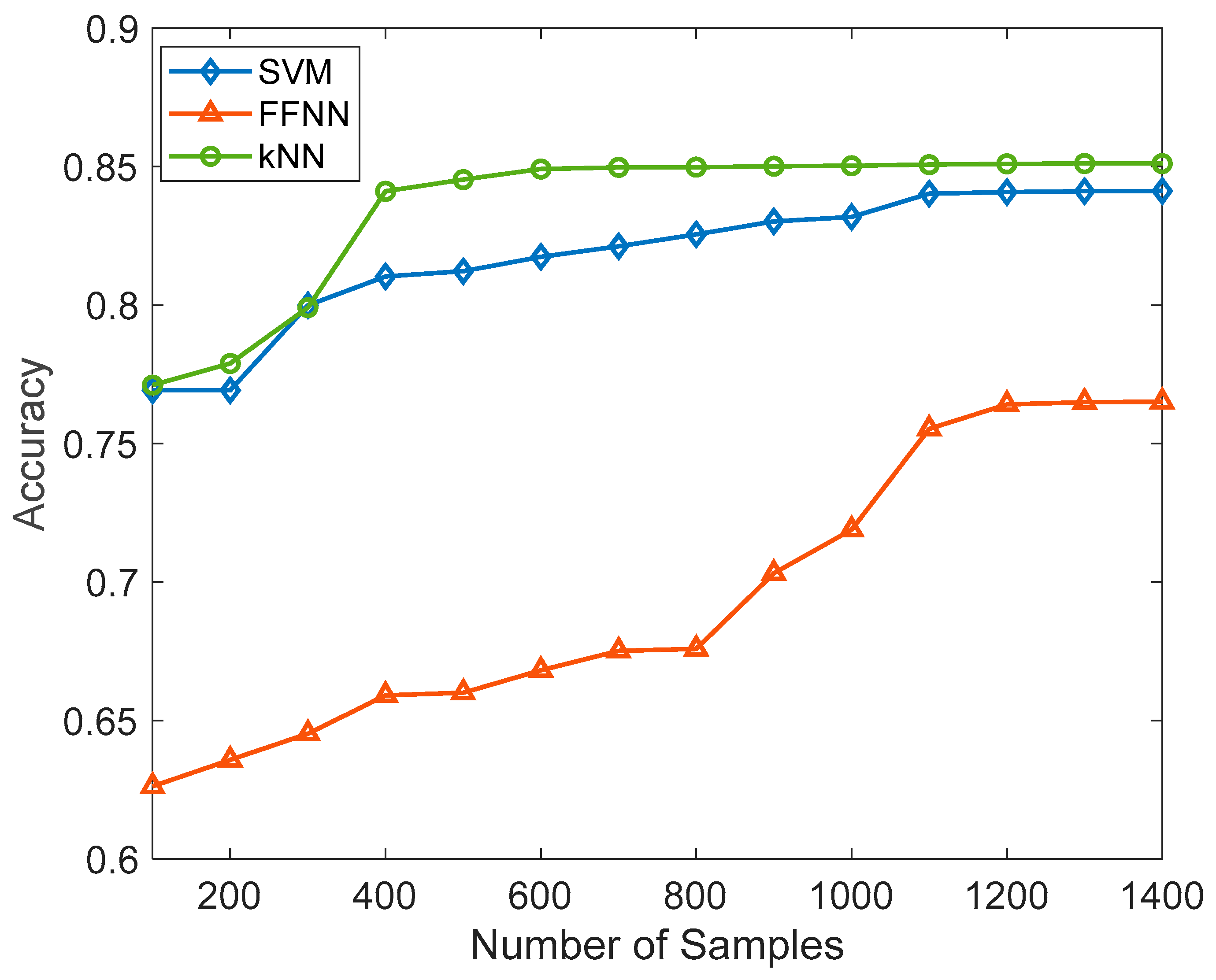
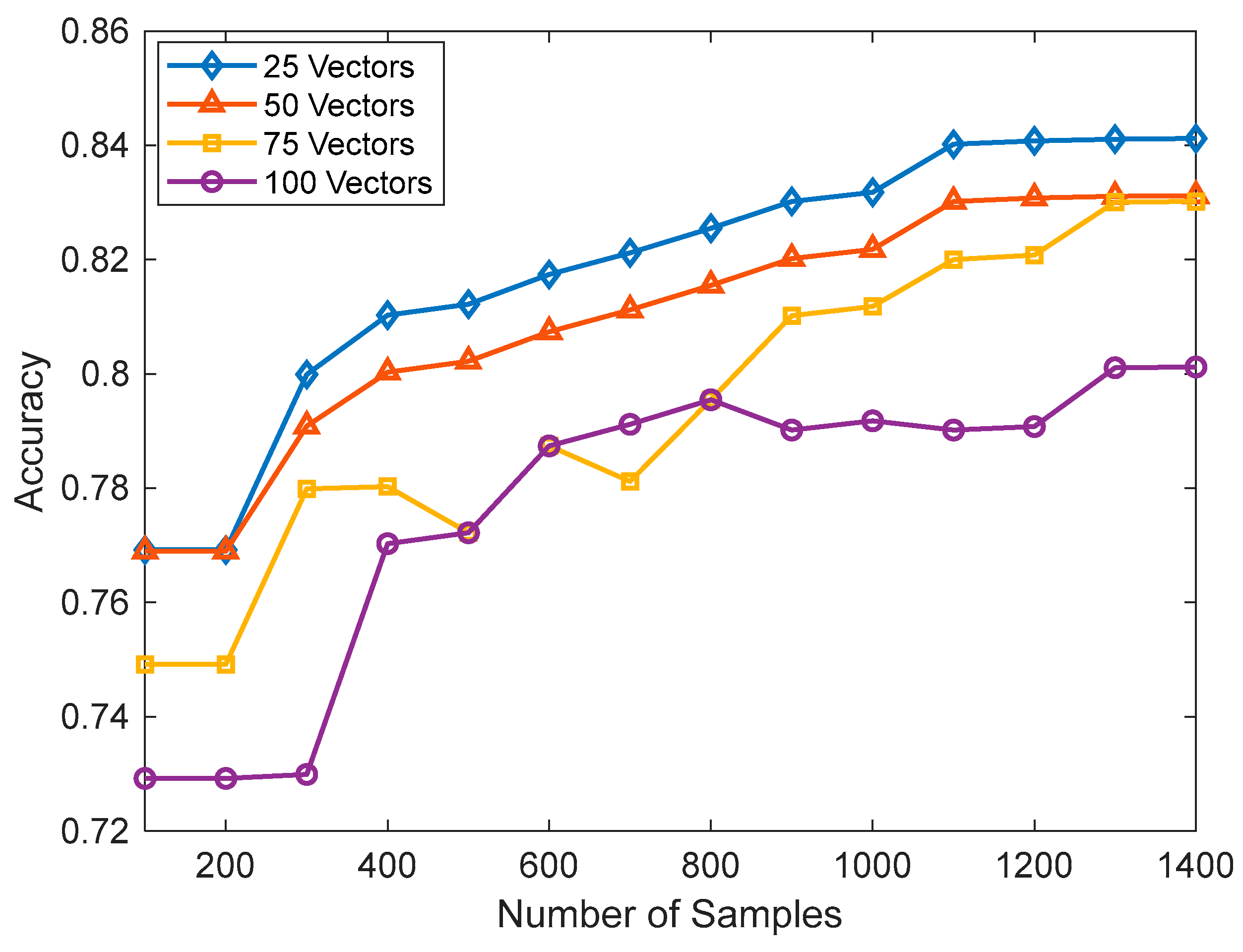
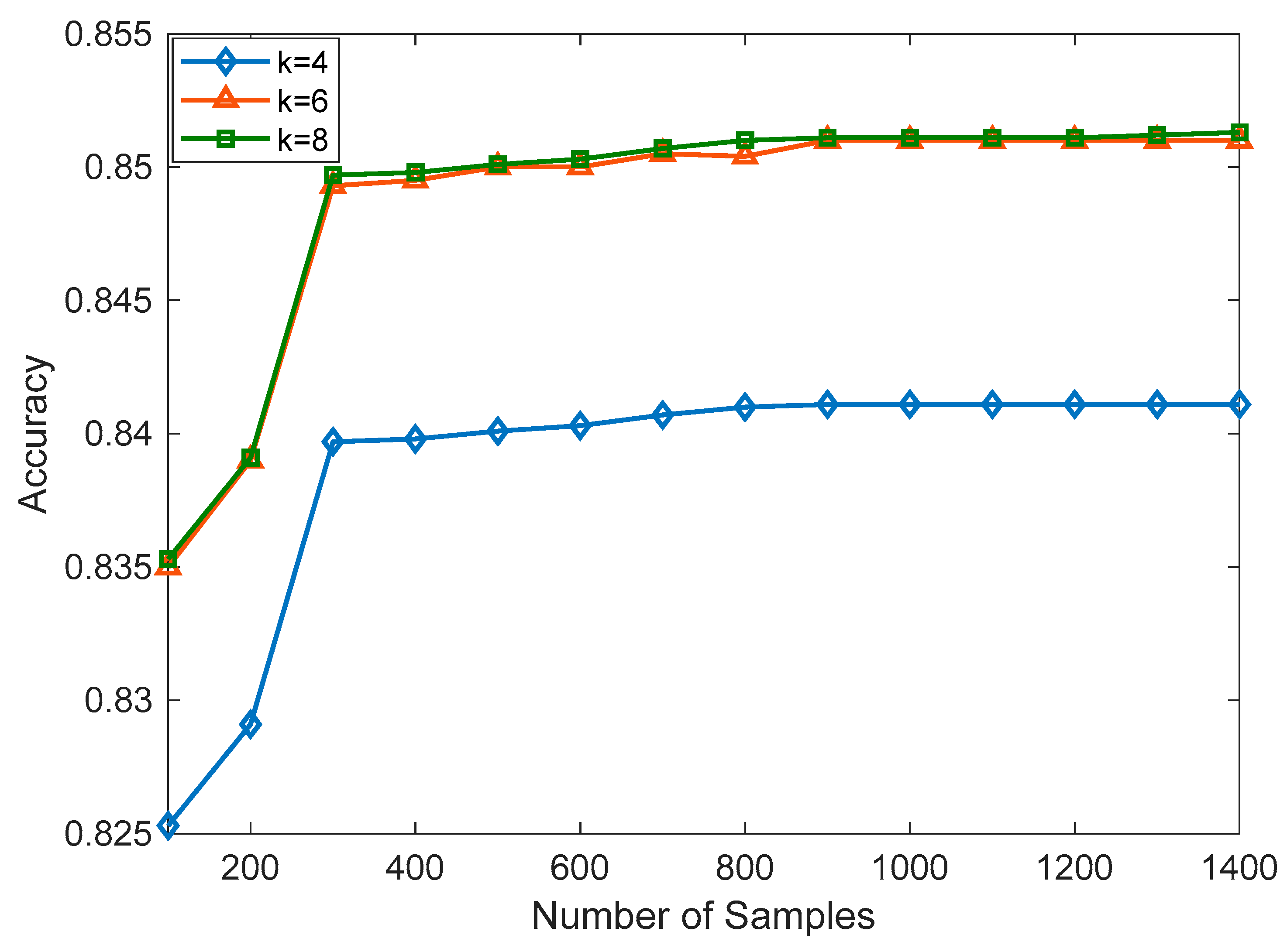
In SVM, the choice of kernel function determined the mapping of data into a higher-dimensional space; here, we used a linear kernel, and the regularization parameter(C) was set to 0.01. The most important hyperparameter to consider when making predictions in k-NN was the number of nearest neighbors. It determines the size of the neighborhood used to classify or regress new data points. We kept k as 5 during our experiment. Both the SVM and kNN were trained using a Jypiter notebook and Python 3 programming language. To build the model, the scikit learn and Pandas library were used. The models were built on an Intel (R) Core (TM) i5-10210U CPU @ 1.60 GHz 2.11 GHz personal computer. During training, the dataset of 5191 was split as 70% for training and 30% for testing. The linear kernel was used for SVM, and the number of vectors was set as 25 in the initial phase. Further, the number of vectors was increased in the model so we could observe the effect of the number of vectors on the accuracy. Initially, the k value of kNN was set to be 4, and we gradually increased the value of k to observe the changes in the accuracy. Further, we also happened to experiment with Logistic Regression (LR), Decision Tree Classifier (DTC), and Random Forest Classifier (RFC). LR yielded an accuracy of 54.2%, DTC demonstrated 76.4% accuracy, and RFC achieved 78.7% accuracy.

All the algorithms evaluated the accuracy, precision, sensitivity, and F1 score. In SVM, the number of support vectors changed from 25 to 75 as a hyperparameter tuning.

5. Results and Discussion

5.1. Results

For all the algorithms, FFNN, SVM and kNN, we calculated the performance evaluation matrices, precision, recall, and the f1-score, in each zone. Finally, we calculated the matrices of the entire dataset. The general definitions for each performance evaluation matrix are as follows:

$$Accuracy=\frac{TP+TN}{TP+FP+FN+TN}$$

(15)

$$Precision=\frac{TP}{TP+FP}$$

(16)

$$Sensitivity=\frac{TP}{TP+FN}$$

(17)

$$F1\text{-}Score=\frac{2\times (Sensitivity\times Precision)}{Sensitivity+Presition}$$

(18)

Without linearization and filtering, the model provided overall accuracies of approximately 77% for KNN, 70% for SVM and 42% for FFNN. Once the filters and linearization were applied, the precision of the FFNN varied from 0.50 to 0.71, the SVM from 0.75 to 0.88, and the kNN from 0.78 to 0.96. Additionally, for the recall, the FFNN was from 0.40 to 0.76, the SVM was from 0.74 to 0.90, and the kNN was from 0.81 to 0.96. For output-sensitive estimation such as localization, we required a high precision and recall. Overall, all the algorithms had over 83% precision and over 76% accuracy in location estimation. The zone-wise precision, recall and f1-score for the FFNN and SVM are presented in Table 4 and Table 5, respectively, where the linear kernel used in the SVM had a gamma value of 0.001 and regularization parameter of 0.01. Table 6 shows the estimation performance zone-wise for the KNN algorithm.

Table 4. FFNN.

Zone	Precision	Recall	f1-Score
Zone A	0.71	0.76	0.73
Zone B	0.50	0.46	0.48
Zone C	0.81	0.85	0.83
Zone D	0.70	0.76	0.72

Table 5. SVM.

	Precision	Recall	f1-Score
Zone A	0.75	0.83	0.79
Zone B	0.89	0.74	0.81
Zone C	0.90	0.85	0.87
Zone D	0.88	0.90	0.89

Table 6. KNN.

	Precision	Recall	f1-Score
Zone A	0.78	0.81	0.79
Zone B	0.88	0.91	0.89
Zone C	0.89	0.87	0.88
Zone D	0.96	0.96	0.96

Previous studies have not paid much attention to hyperparameter tuning. This may have led to low accuracy in the location estimation being provided. Related works show some low accuracies, such as 50–60% in algorithms, due to the number of samples in the dataset and the due unavailability of RSSI filtering [18,19,20]. During the experiments, we considered the hyperparameter tuning of the SVM, kNN, and FFNN algorithms. For the SVM, the number of vectors was increased from 25 to 75. It can be observed that accuracy improves when the number of vectors in the SVM increases. Table 7 denotes the summary of performance for each algorithm. When increasing the vectors, it was observed that there was a significant improvement in the accuracy and f1-score. Overall, the kNN gave 0.8511 accuracies, and it outperformed the other algorithms.

Table 7. Performance comparison of all the machine learning algorithms.

Algorithm		Sensitivity	Specificity	Precision	Accuracy	f1-Score
FFNN		0.8976	0.5176	0.8344	0.7651	0.6949
SVM	Vectors = 25	0.9083	0.5176	0.8505	0.8401	0.8479
	Vectors = 50	0.9083	0.5176	0.8505	0.8408	0.8480
	Vectors = 75	0.9083	0.5176	0.8505	0.8412	0.8485
KNN		0.9587	0.4215	0.9062	0.8511	0.8817

For FFNN, we adjusted the hyper-parameters, including the learning rate, batch size, and the number of epochs. It was observed that the training accuracy was consistently higher than the testing accuracy. Three distinct batch sizes, 10, 50, and 100, were used to test the training and testing accuracy. The epochs ranged from 0 to 100. Figure 4 and Figure 5 display the outcomes. The kNN operates based on its proximity to training examples. In cases where the decision boundary is not highly complex and can be approximated well by a set of local regions, kNN can be effective. The FFNN and SVM might introduce unnecessary complexity in such scenarios. The practicality of implementing machine learning algorithms like the FFNN, k-NN, and SVM on IoT edge devices depends on factors like model complexity, computational resources, memory constraints, and the specific use case. While lightweight algorithms like k-NN are generally well-suited for edge deployment, more complex models like FFNN and SVMs may require careful optimization and the consideration of resource limitations. Additionally, model quantization, pruning, and approximate algorithms can be used to improve the feasibility of these algorithms on IoT edge devices.

Figure 5. Training accuracy vs. number of epochs.

5.2. Training Time

Figure 6 shows the association between the number of samples and the training time for all three algorithms. When the number of samples increases, all the algorithms’ training times increase, where kNN shows the lowest training time while FFNN gives the highest training time. It was observed that from 200 samples to 1200 samples, the training time increased exponentially. Additionally, after 1200 samples, it showed stableness. When comparing the training time of FFNN, it was higher compared to the other algorithms tested. This could be due to the computational complexity of the neural network. To overcome this, the stochastic gradient descent can be proposed. Stochastic gradient descent works by randomly selecting a small number m, chosen haphazardly training inputs. The kNN showed less training time because it does not learn a discriminative function from the training data.

Figure 6. Training time vs. various machine learning algorithms.

5.3. Accuracy

Figure 7 shows the correlation between the number of samples versus the accuracy. The accuracy rose as the number of samples increased for all the algorithms. In an FFNN up to 1000 samples, the accuracy increased exponentially. Additionally, after 1000 samples, accuracy became sort of saturated. However, the FFNN provides the lowest accuracy compared to the other two algorithms. The smaller number of data points could be a reason for it showing the lowest accuracy in the FFNN. In the SVM and kNN, up to 200 samples, we could see a significant increment of accuracy. However, after 200 samples, we saw less of an increment. The reduction of model overfitting can be used to explain the accuracy versus the training dataset size curve. In general, as the amount of the training dataset increases, model overfitting considerably decreases.

Figure 7. Accuracy vs. various machine learning algorithms.

5.4. F1-Score

Figure 8 shows the relationship between the number of samples and the f1-score. By computing the harmonic mean of a classifier’s precision and recall, the f1-score assimilates both into a single metric. It is mainly used to compare the effectiveness of two classifiers. As per the results, the f1-score also rapidly upsurged as the number of samples increased. According to the results, the kNN gave the highest f1-score, and the FNN offered the lowest value. Generally, the accuracy was suitable for a balanced dataset. However, the utilized dataset in this work was an imbalanced dataset, where we had an unequal number of data samples for four Zones A, B, C, and D. Since the dataset had an imbalance, the matrix f1-score was more suitable for evaluating this model.

Figure 8. f1-score vs. various machine learning algorithms.

5.5. Accuracy with Number of Vectors

Figure 9 shows the relationship between the accuracy, number of samples, and vectors. When the number of samples increases, accuracy increases irrespective of the number of vectors. When the number of vectors increases, accuracy sees a significant reduction. We considered the linear kernel SVM in this experiment. Additionally, improving the classifier’s performance did not always result in the addition of more support vectors. The trade-off between accuracy and the number of support vectors that we previously considered true did not always hold in this specific situation. If there were already more than a particular number of support vectors—in this case, about 110—then adding another support vector resulted in declining marginal returns.

Figure 9. Accuracy vs. number of samples, with different number of vectors.

5.6. Accuracy vs. k Value in kNN

Figure 10 shows the effect of the k value in the kNN on the accuracy. When k increased from 2 to 6, we can observe an exponential increment in accuracy. Additionally, from 6 to 20 the accuracy increased. A low number of k indicates that noise will have a more significant impact on the outcome. A considerable value makes it computationally expensive and somewhat contradicts the fundamental tenets of KNN.

Figure 10. Accuracy vs. number of samples with different k values.

6. Conclusions

This paper presented a simplified localization method based on BLE and supervised ML classifiers that could apply in robust indoor localization applications. Since the proposed localization method is based on ML, it could be easily deployed in practical environments as the ML model could run on tiny embedded systems. The RSSI values were collected from thirteen different iBeacon nodes installed in an indoor environment utilized in this experiment. The RSSI data were linearized using the weighted least-squares method and filtered using moving average filters to remove the outliers. Afterward, RSSI data were trained using the SVM, kNN, and FFNN algorithms. During the experiments, each algorithm’s hyperparameters were tuned, and the impact on its accuracy was observed. It was observed that there were significant improvements in the accuracy once the sample size was increased. Further, training time was observed against the sample size and the number of epochs versus accuracy. The training time increased as the number of samples increased. Further, accuracy had a significant improvement once the epoch size increased. Overall, the kNN offers reasonably good accuracy in classifying the right zone of 85%, the FFNN provides 76% when the batch size is 100, under a learning rate of 0.01, and the SVM provides 84% with 75 support vectors.