Article

Application of Machine Learning Techniques for Predicting Students’ Acoustic Evaluation in a University Library

1
Department of Building Environment and Energy Engineering, The Hong Kong Polytechnic University, Hong Kong, China
2
Department of Architecture and Industrial Design, Università degli Studi della Campania “Luigi Vanvitelli”, 81031 Aversa, Italy
*
Author to whom correspondence should be addressed.
Acoustics 2024, 6(3), 681-697; https://doi.org/10.3390/acoustics6030037
Submission received: 29 May 2024 / Revised: 10 July 2024 / Accepted: 23 July 2024 / Published: 25 July 2024
(This article belongs to the Special Issue Acoustical Comfort in Educational Buildings)

Abstract

:
Understanding students’ acoustic evaluation in learning environments is crucial for identifying acoustic issues, improving acoustic conditions, and enhancing academic performance. However, predictive models are not specifically tailored to predict students’ acoustic evaluations, particularly in educational settings. To bridge this gap, the present study conducted a field investigation in a university library, including a measurement and questionnaire survey. Using the collected personal information, room-related parameters, and sound pressure levels as input, six machine learning models (Support Vector Machine–Radial Basis Function (SVM (RBF)), Support Vector Machine–Sigmoid (SVM (Sigmoid)), Gradient Boosting Machine (GBM), Logistic Regression (LR), Random Forest (RF), and Naïve Bayes (NB)) were trained to predict students’ acoustic acceptance/satisfaction. The performance of these models was evaluated using five metrics, allowing for a comparative analysis. The results revealed that the models better predicted acoustic acceptance than acoustic satisfaction. Notably, the RF and GBM models exhibited the highest performance, with accuracies of 0.87 and 0.84, respectively, in predicting acoustic acceptance. Conversely, the SVM models performed poorly and were not recommended for acoustic quality prediction. The findings of this study demonstrated the feasibility of employing machine learning models to predict occupants’ acoustic evaluations, thereby providing valuable insights for future acoustic assessments.

1. Introduction

1.1. Importance of Acoustic Quality in Learning Environments

Acoustic quality plays a crucial role in creating an optimal learning environment. It can significantly impact students’ health [1] and well-being [2]. High noise levels can decrease students’ cortisol variability and result in stress, fatigue, and headaches [1,3]. Furthermore, long reverberation time also can hurt students’ well-being [4,5] and reduce their happiness [6]. Long exposure to such environments may further affect students’ cognitive processing and epistemic motivation [7].
Moreover, acoustic comfort is closely related to students’ academic performance, particularly in relation to their listening comprehension [8]. Various studies have revealed that different types of noise have detrimental effects on students’ listening comprehension, with speech distractors having the greatest negative impact [9,10]. Notably, the impacts were more obvious for non-native speakers and during higher-level comprehension tasks [10,11]. Additionally, noise also hampers students’ numeracy, reading, and writing abilities due to its potential to disrupt attention control, thereby impeding cognitive processes necessary for these tasks [12,13].
Considering the effectiveness of acoustic quality on students’ health, well-being, and learning performance, ensuring a comfortable acoustic environment in learning spaces is paramount. To achieve this, the initial and primary step is to effectively evaluate the acoustic quality in learning environments and identify areas that exhibit poor acoustic conditions. Subsequently, targeted renovations can be implemented to improve the acoustic quality in the identified areas.

1.2. Prediction of Acoustic Quality in Learning Environments

Acoustic measurement and evaluation are time-consuming and device-demanding, especially the measurement of reverberation time and the questionnaire survey. Therefore, many previous studies have only measured sound pressure level as the indicator of acoustic quality [14,15], and several studies proposed regression models to evaluate occupants’ acoustic comfort only based on this indicator [16,17,18]. For example, Yang and Mak [17] and Cao et al. [18] established linear regression models to predict occupants’ acoustic satisfaction based on the A-weighted sound pressure level. Wong et al. [19] developed a logistic regression model to quantify the impact of noise level on occupants’ acoustic acceptance. Regression analysis, including linear and logistic regression, is renowned for its simplicity and ease of comprehension. Nevertheless, it is important to acknowledge that the accuracy of regression models may be limited due to their sensitivity to outliers and influential points. Consequently, exploring and employing more advanced techniques to mitigate these limitations is advisable to develop more accurate prediction models.

1.3. Application of Machine Learning for Prediction of Indoor Environment Quality

The development of machine learning techniques has revolutionized the prediction of indoor environmental quality (IEQ). By leveraging large amounts of data and complex algorithms, machine learning models can accurately predict the specific quality of the investigated environments. Many studies have tested different algorithms predicting IEQ in the past five years. However, most of these studies focused on thermal comfort and indoor air quality (IAQ) [20,21,22,23]. For example, Luo et al. [22] established nine machine learning models using the ASHRAE Global Thermal Database to predict occupants’ thermal sensation votes. Wong et al. [20] employed nine classification models to assess indoor air quality. All these studies demonstrated machine learning models’ ability to accurately predict the quality of environmental factors.
Nonetheless, regarding the application of machine learning in acoustic-related pre-diction, studies are relatively limited. Most of these studies focused on the acoustic quality of vehicles, for example, the sound quality prediction in different types of cars [24], the sound insulation evaluation in high-speed trains [25], and occupants’ acoustic comfort prediction in buses [26]. Additionally, some studies utilized machine learning for acoustic prediction in buildings. For instance, Yeh and Tsay [27] used four machine learning algorithms to predict acoustic-related indicators, such as sound pressure level and speech transmission index in Multi-Functional Activity Centers, based on the geometric information and material properties; Bonet-Solà et al. [28] employed convolutional neural network (CNN) and logistic regression to evaluate the acoustic comfort of dwellings based on the 30 s video of acoustic events recorded onsite; and Puyana-Romero et al. [29,30] applied different models to predict students’ acoustic satisfaction and online learning performance at home. However, to the best of the authors’ knowledge, no study has yet applied the machine learning algorithm to predict students’ acoustic comfort in educational buildings, and no studies have compared how different algorithms and feature selection can influence prediction accuracy.

1.4. Research Questions of the Current Study

Therefore, the primary objective of this study is to explore the feasibility of employing machine learning techniques in predicting students’ acoustic evaluations within a university library setting. Specifically, this study aims to address the following two research questions:
  • Which variables will likely influence students’ acoustic evaluations of a learning space?
  • Which predictive models demonstrate the highest accuracy in forecasting students’ acoustic evaluations?
By answering these questions, it will be possible to identify an accurate model capable of predicting students’ acoustic evaluations and, in turn, that can facilitate assessing and enhancing acoustic quality in learning environments.

2. Materials and Methods

Figure 1 illustrates the overall process of this study. First, a field study was carried out in a university library to collect data. Then, data analyses were conducted to select potential predictors of students’ acoustic evaluations. Lastly, several machine learning models were trained and compared to predict students’ acoustic assessment. Each step will be explained in detail in the following subsections.

2.1. Data Collection

The field study, including on-site measurement and questionnaire survey, took place in four study rooms of a university library in Hong Kong for weekdays from 19 October to 1 November 2022. These rooms consisted of two group study rooms where students could discuss their studies and two self-study rooms where students were required to keep silent.
Four EVQ SENSEs integrated IEQ sensors (Annecy Solutions Limited, Central, Hong Kong) were utilized for the on-site measurement to measure the A-weighted sound pressure level (SPL) every minute during the investigation period, specifically from 9:00 to 18:00 each day (see Figure 2). Following the sampling process recommended by CIBSE (Chartered Institution of Building Services Engineers) [31], the sensor was placed at the center of each study room on top of a desk (1.1 m in height). Before this study, the four devices were compared with a calibrated sound level meter—RS PRO DT-8852 (RS PRO, London, UK)—in an office environment. No significant differences in sound pressure levels (SPLs) were identified between the devices, indicating their validity.
During the measurement, students studying in the investigated rooms for at least 30 min were randomly asked (maximum once) to participate in the questionnaire survey. Four researchers, each stationed in one room, were responsible for distributing and collecting the questionnaires. The questionnaire comprised several parts; however, only the personal and room information (i.e., gender, age, current feeling, seat location, and room type) and the evaluation of acoustic quality were exported and analyzed in the present paper. Regarding the question on current feelings (i.e., “How are you feeling now”), the answers were Good/Neutral/Bad, coded as 1/0/−1; for the questions on seat location (i.e., “Where do you sit in the room”), the answers were Middle/Others, coded as 1/0; and for the question on acoustic evaluation (i.e., “How satisfied are you with this acoustic environment”), a 7-point Likert scale was used, and the answers from totally dissatisfied to neutral to totally satisfied were coded as −3 to 0 to 3. The room types were also recorded by the researchers. The group study rooms were coded as 1 and the self-study rooms were coded as 0.
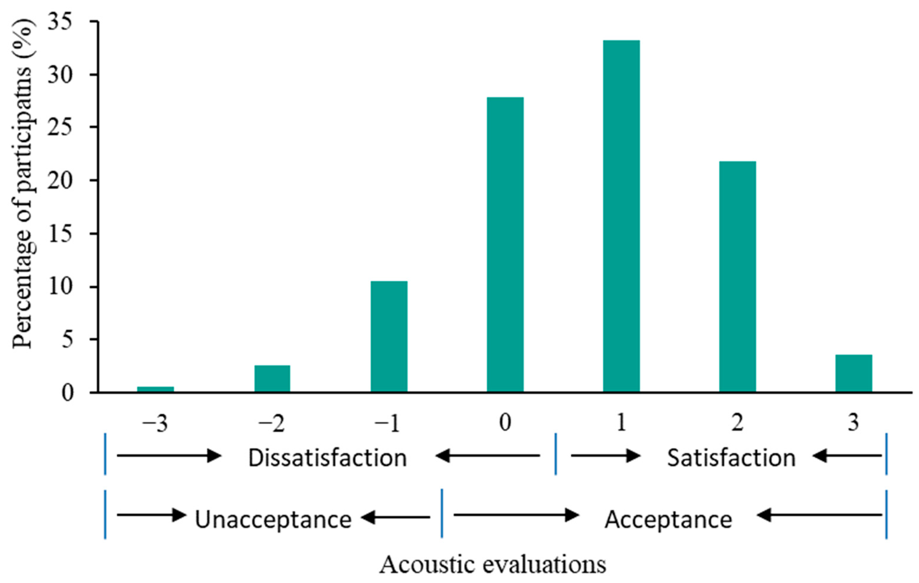
Previous studies have treated the concept of “neutral” differently when evaluating IEQ [32,33]. As indicated by Karmann et al. [34], different studies and standards adopted different ranges of the 7-point scales (i.e., from neutral to very satisfied or from slightly satisfied to very satisfied) as “satisfied” conditions, because of the different judgements between satisfaction and acceptability. Since there is no unified method regarding the satisfaction metrics, this study provided two ways to analyze this parameter: acoustic satisfaction (exclude neutral) and acoustic acceptance (include neutral). Although the terms “satisfaction” and “acceptance” have different definitions in the dictionary, they have sometimes been used interchangeably in previous studies [35,36]. This variation in usage often depends on the specific context and the authors’ interpretations. In the current study, as shown in Figure 3, these two sets of terms were defined as follows:
  • Acoustic Dissatisfaction: answers from “totally dissatisfied (−3)” to “neutral (0)”;
  • Acoustic Satisfaction: answers from “slightly satisfied (1)” to “totally satisfied (3)”;
  • Acoustic Unacceptance: answers from “totally dissatisfied (−3)” to “slightly dissatisfied (−1)”;
  • Acoustic Acceptance: answers from “neutral (0)” to “totally satisfied (3)”.
By providing these two ways of analyzing the satisfaction metric, this study aims to offer a more comprehensive understanding of the relationship between acoustic conditions and occupant satisfaction.

2.2. Data Analysis

The collected data were imported into IBM SPSS 26.0 for the primary analyses. First, the data were cleaned by screening outliers identified by Z-scores of the SPLs. The cases where the absolute values of the Z-scores exceeded three were excluded from the analysis.
After that, the 15 min A-weighted equivalent sound pressure level was calculated based on the SPLs using Equation (1), as this is the most common environmental noise descriptor [37].
L A e q = 10 log 10 1 n i = 1 n 10 S P L i 10
where n is the number of samples in the targeted interval, namely 15 min, and S P L i is ith sampled SPL in dB(A). Also, LA90 and LA10 were calculated to represent the background noise and the sporadic loud noise levels, as they defined the A-weighted sound level which exceeded for 90% or 10% of the measurement period.
Then, the relationships between the acoustic acceptance/satisfaction and the variables at the interval/ratio level (i.e., age and body mass index (BMI)) were checked by independent t-tests; relationships between the SPL and the variables at the nominal/ordinal level (i.e., room type, seat location, gender, and feeling) were checked by Chi-square tests. All the variables that might potentially influence acoustic acceptance/satisfaction (p < 0.1) were selected as the indicators in the machine learning models.

2.3. Machine Learning

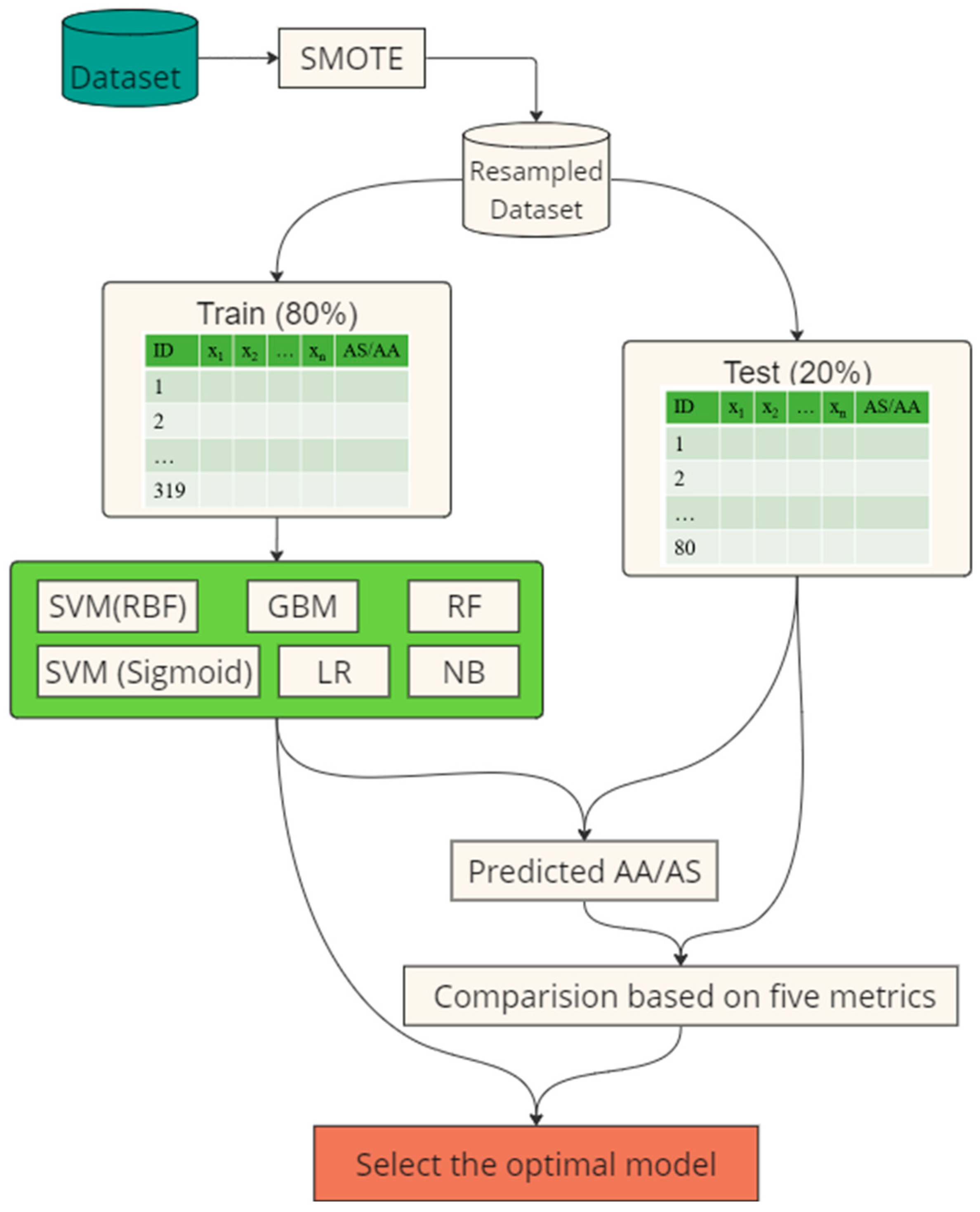
The process of the model development and selection is shown in Figure 4. Before the development of the models, the Synthetic Minority Over-sampling Technique (SMOTE) was applied to address the imbalances in the predicted binary classifications. SMOTE is a widely used over-sampling technique that generates synthetic samples for the minority class by interpolating between existing minority class examples [38]. It efficiently deals with imbalanced datasets [39,40]. The current study used SMOTE to generate new cases that closely resemble the dataset’s acoustic unacceptance/dissatisfied cases. After this process, the dataset expanded to 688 cases for the acoustic acceptance prediction and 466 cases for the acoustic satisfaction prediction.
The training data and testing data were randomly selected at a distribution ratio of training data (80%) and testing data (20%). Based on previous studies in the field of IEQ, the following six ML techniques were applied in the current study to predict students’ acoustic acceptance/satisfaction in a library.
  • Support Vector Machine–Radial Basis Function (SVM (RBF)): SVM (RBF) is a popular kernel-based classification algorithm that can handle non-linear and high-dimensional data. The radial basis function (RBF) kernel is a common choice for SVM, which maps the data into a high-dimensional space using a Gaussian function. SVM (RBF) is relatively sensitive to model parameters [41].
  • Support Vector Machine–Sigmoid (SVM (Sigmoid)). SVM (Sigmoid) is another variant of SVM, and it is also a powerful technique to handle non-linear data. Unlike the SVM (RBF), SVM (Sigmoid) uses the hyperbolic tangent function to map the data [41].
  • Gradient Boosting Machine (GBM): GBM is an ensemble technique that builds models sequentially, where each new model aims to improve the previous ones. It combines the predictions of multiple weak learners (usually decision trees) to produce a strong model [42].
  • Logistic Regression (LR): LR is a statistical model used for binary classification based on one or more predictor variables. As indicated by its name, LR uses the logistic function to map data [43].
  • Random Forest (RF): RF is also an ensemble learning method that constructs multiple decision trees. However, unlike FBM, RF builds trees independently and relies on averaging prediction, leading to high robustness [44].
  • Naïve Bayes (NB): NB is a probabilistic classifier based on Bayes’ theorem. NB assumes independence between predictors, which is efficient but might result in less accurate outcomes [45].
Then, these models were applied to predict students’ acoustic acceptance/satisfaction using the test data. The differences between the predicted and collected results were used to calculate the models’ accuracies and evaluate their performance. According to the evaluation metrics of these models, the optimal prediction model could be identified.
In terms of the evaluation metrics, five commonly used indicators were considered in the current study: accuracy, sensitivity, precision, specificity, and F1 score. Accuracy represents the percentages of the correctly predicted cases in the tested dataset (see Equation (2), where TP, TN, FP, and FN represent true positives, true negatives, false positives, and false negatives of the model’s predictions, respectively). Sensitivity, known as the true positive rate, represents the proportion of correctly predicted positive cases among all the actual positive cases (see Equation (3)); precision represents the percentage of correctly predicted acceptance cases among all the cases that were predicted as acceptance (see Equation (4)); specificity, known as the true negative rate, represents the proportion of correctly predicted negative cases among all the actual negative (see Equation (5)); F1 score represents the combination of sensitivity and precision, and it is calculated as the harmonic mean of sensitivity and precision (see Equation (6)). For all these indicators, higher values typically indicate better performance of the models.
A c c u r a c y = T P + T N T P + T N + F P + F N
S e n s i t i v i t y = T P T P + F N
P r e c i s i o n = T P T P + F P
S p e c i f i c i t y = T N T N + F P
F 1 = 2 × S e n s i t i v i t y × P r e c i s i o n S e n s i t i v i t y + P r e c i s i o n

3. Results

3.1. Predictor Selection

In total, 404 questionnaires were collected in the field study, and six were excluded because of the incompletion of the necessary questions (i.e., the acoustic perceptions). Therefore, 398 questionnaires were considered valid and analyzed in the current study.
Table 1 shows the general information of the occupants’ personal information, room-related indicators, and dose-related acoustic variables. According to the collected questionnaires, the proportions of females (48%) and males (52%) were relatively balanced; most students felt good during the survey; their BMIs were generally within the healthy range recommended by WHO; there were more students in the group-study rooms (57%) than in the self-study rooms (43%); and about half of the students sat in the middle spots in the investigated room.
In addition, the measurement results indicated that the average LAeq in these rooms was 50.1 dB(A), the average LA10 was 51.1 dB(A), and the average LA90 was 49.1 dB(A). It should be noted that the LA10 and LA90 were calculated every 15 min, which explains why the difference between them was minimal. Considering the entire investigated period, the LA10 was 56.5 dB(A), and the LA90 was 40.0 dB(A). The result indicates that the sound pressure level (SPL) was lower than 40.0 dB(A) for 90% of the investigated period.
In order to select the factor for predicting students’ acoustic acceptance/satisfaction in the investigated room, a series of t-tests and Chi-square tests were conducted, and results are also shown in Table 1. The potential predictors of acoustic acceptance were age, gender, feeling, room type, and seat location. Additionally, LAeq was selected as the representative of the dose-related indicator, considering its relatively lower p-value among the three acoustic indicators. Regarding acoustic satisfaction, its potential predictors include age, feeling, BMI, and all the acoustic indicators. However, since LAeq, LA10, and LA90 were all calculated based on SPL [46], only LAeq was selected (because of its relatively lower p-value) to avoid the intercorrelations between the predictors.
Figure 5 illustrates students’ evaluations of the acoustic quality in the investigated learning environment. As shown in this figure, the answers of 58% of occupants were positive (1 to 3), 28% were neutral (0), and only 15% were negative (−1 to −3). Considering the large proportion of “neutral”, which cannot be ignored, and the inconsistent classification regarding the “neutral” choice in previous studies, as mentioned in Section 2.1, this study applied two modes of analyzing this variable: acoustic satisfaction (1–3) and acoustic acceptance (0–3). According to the data shown in Figure 4, 58% of occupants were categorized under “acoustic satisfaction”, 42% under “dissatisfaction”, 85% “acoustic acceptance”, and 15% “unacceptance”.

3.2. Acoustic Acceptance Prediction

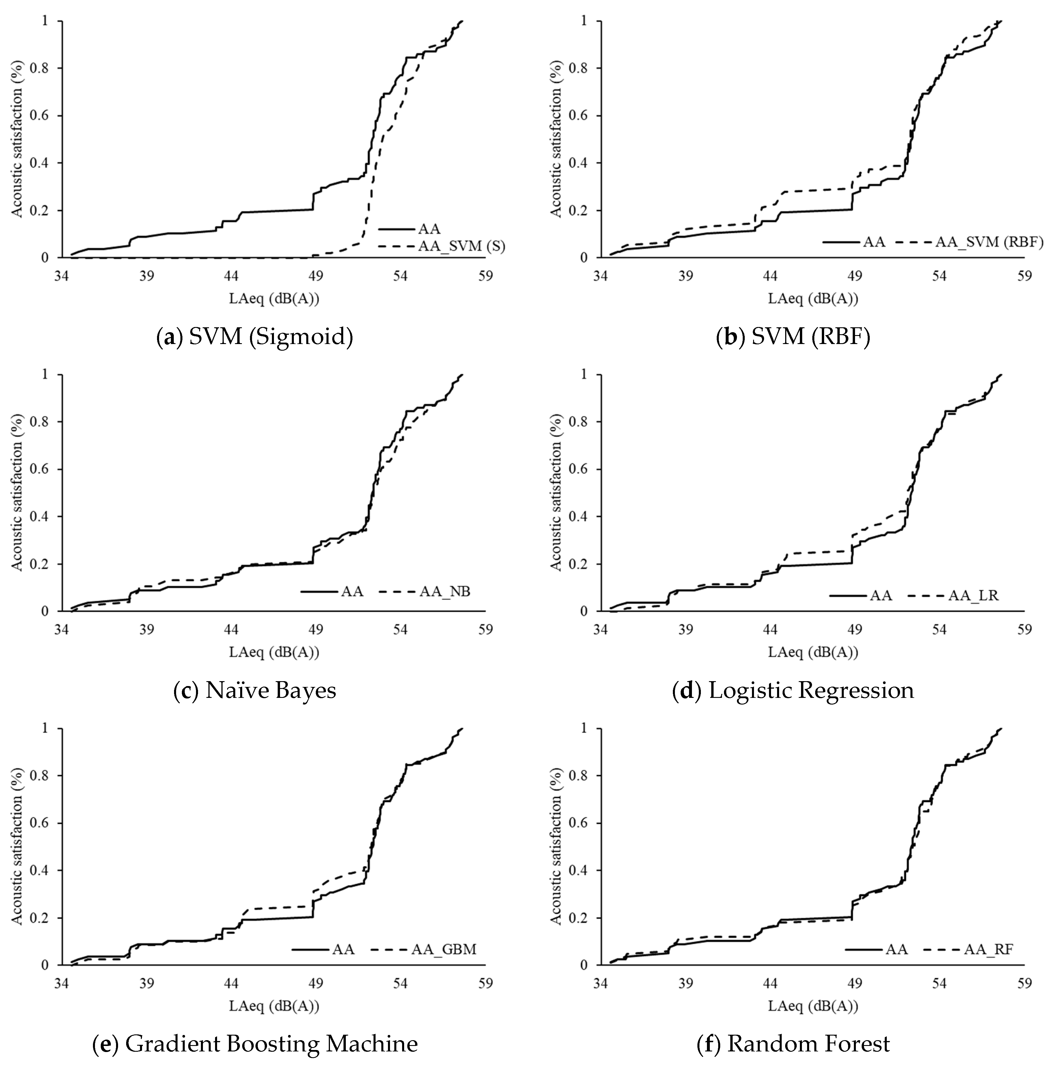
Figure 6 exhibits the predicted and collected acoustic acceptance in the test dataset. Since the dataset expanded to 688 cases for the acoustic acceptance prediction after the over-sampling, the test dataset included 138 cases, namely 20% of the whole dataset. Among the six tested models, SVM (both Sigmoid and RBF) performed the worst (with less than 65% accuracy), followed by NB and LR (with around 75% accuracy), while GBM and RF performed the best (with around 83% accuracy). In addition, according to the Chi-square test results shown in Table 2, the results predicted by almost all these models (except for SVM (Sigmoid)) were significantly correlated with the collected data (p < 0.05).
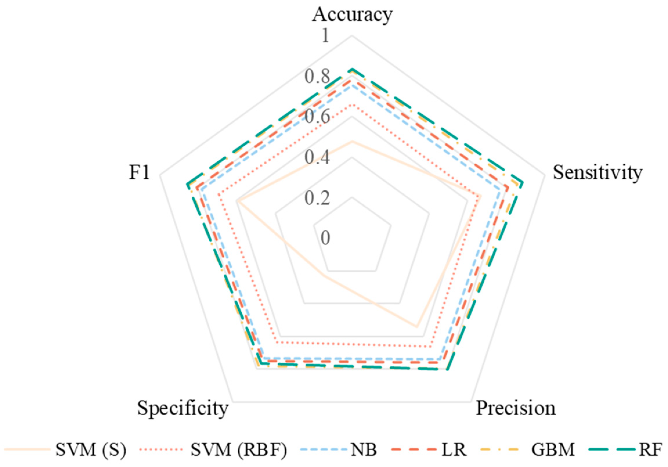
Regarding other evaluation indicators, as shown in Figure 7, the ranking among these models was almost the same as the ranking of accuracy. Specifically, RF and GBM consistently outperformed the others. They achieved high scores across all metrics—accuracy, sensitivity, precision, specificity, and F1—indicating strong discrimination ability and a good balance between precision and sensitivity. This comprehensive performance indicates that RF and GBM are highly effective in correctly classifying positive and negative instances, making them reliable choices for predictive students’ acoustic acceptance. The NB and LR performed reasonably well. Both models exhibited relatively high accuracy and demonstrated a balanced performance in terms of precision and sensitivity. NB and LR showed moderate effectiveness in identifying true positive and true negative cases, suggesting that they can still be valuable in practical applications where a simpler model may be preferred for computational efficiency. In contrast, the two SVM models showed the poorest performance, especially the one with the Sigmoid kernel, with the lowest scores for all the evaluation indicators. This result indicates that the SVM (Sigmoid) model struggled significantly with classification tasks, failing to effectively discriminate between acoustic acceptance and unacceptance. The SVM (RBF) performed slightly better than the SVM (Sigmoid) but still lagged behind the other models in terms of overall performance.

3.3. Acoustic Satisfaction Prediction

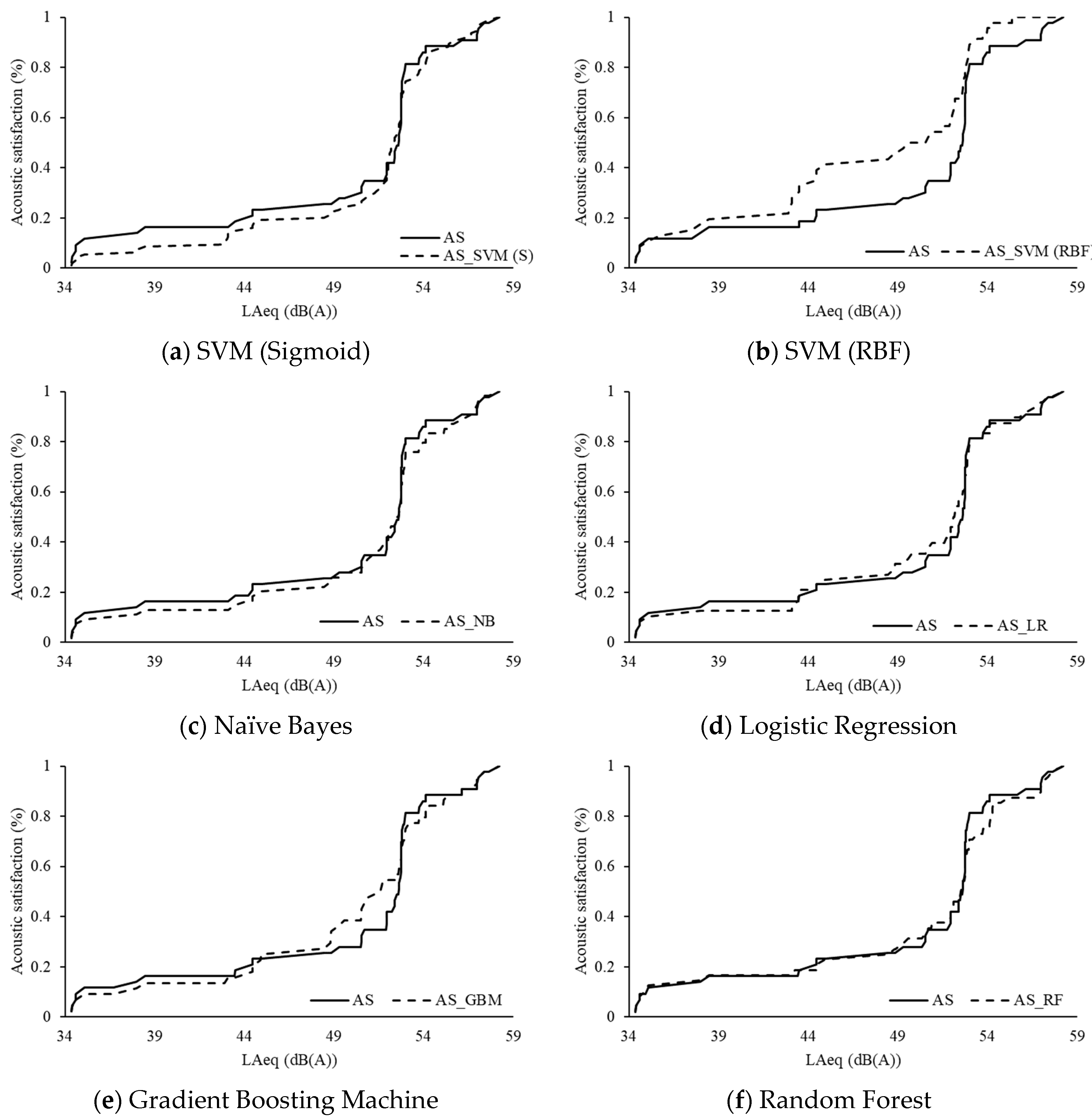
Regarding the prediction of students’ acoustic satisfaction, the accuracies of these models (46–67%) were lower than those of the prediction of their acoustic acceptance (48–83%), as shown in Figure 8. After the over-sampling by SMOTE, the dataset was expanded to 466 cases for the acoustic satisfaction prediction, and thus the test dataset included 94 (20% × 466) cases. Among the six tested models, the SVM (Sigmoid) performed the worst (with less than 50% accuracy) for the prediction of acoustic satisfaction, which was similar to the acoustic acceptance prediction. Next were SVM (RBF) and LR (with around 55% accuracy), while NB, GBM, and RF performed the best (with around 65% accuracy). In addition, according to the Chi-square test results in Table 3, only the NB, GBM, and RF predictions were significantly correlated with the collected data (p < 0.05).
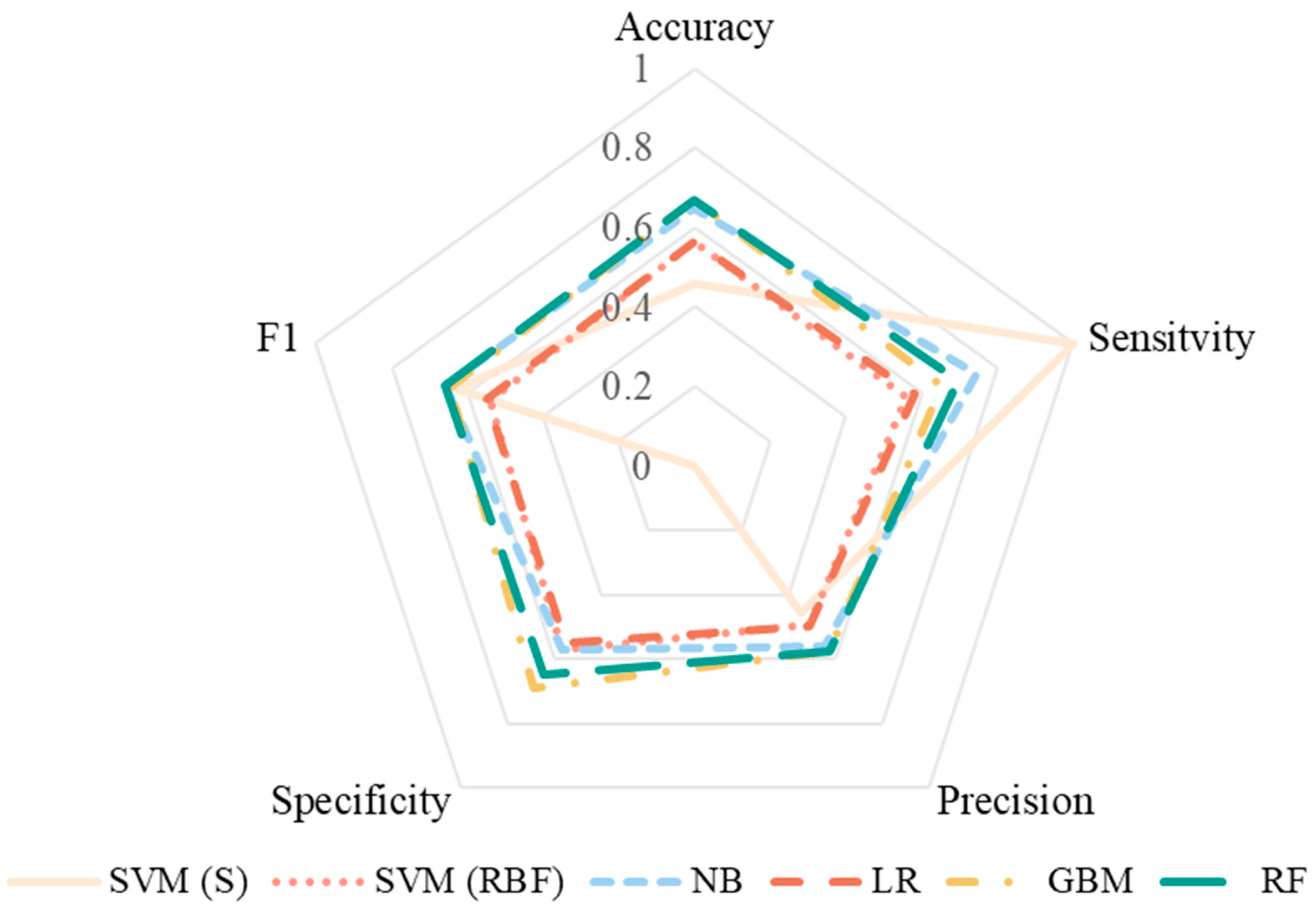
Regarding the evaluation of these models’ performance on acoustic satisfaction prediction, Figure 9 illustrates the related evaluation. Most models demonstrated balanced scores, except for SVM (Sigmoid). This model had a sensitivity of 1 and specificity of 0, indicating a problem with its predictions, since it falsely predicted all the dissatisfied cases as satisfied and resulted in a complete lack of true negative predictions. Apart from that, all the other models achieved relatively balanced scores for these evaluation metrics (0.5–0.7). Moreover, these models’ performances were slightly different than their performance on acoustic acceptance prediction. Specifically, RF, GBM, and NB performed on par with each other, demonstrating the top performance. The NB and SVM (RBF) models showed moderate performance with balanced scores across all the metrics. On the other hand, the SVM (Sigmoid) model exhibited significant imbalances between sensitivity and specificity, making it unsuitable for the acoustic satisfaction prediction.

4. Discussion

4.1. Parameters to Indicate Occupants’ Acoustic Evaluations

The current study focused on two target parameters, acoustic acceptance and acoustic satisfaction, derived from students’ acoustic evaluations. Acoustic satisfaction encompassed options indicating varying satisfaction levels, while acoustic acceptance included the satisfaction options and the additional “neutral” option, allowing for a broader response. Approximately 30% of students selected “neutral” regarding their acoustic satisfaction in the examined rooms. The classification and treatment of these neutral responses could substantially influence the ultimate findings and conclusions of the study.
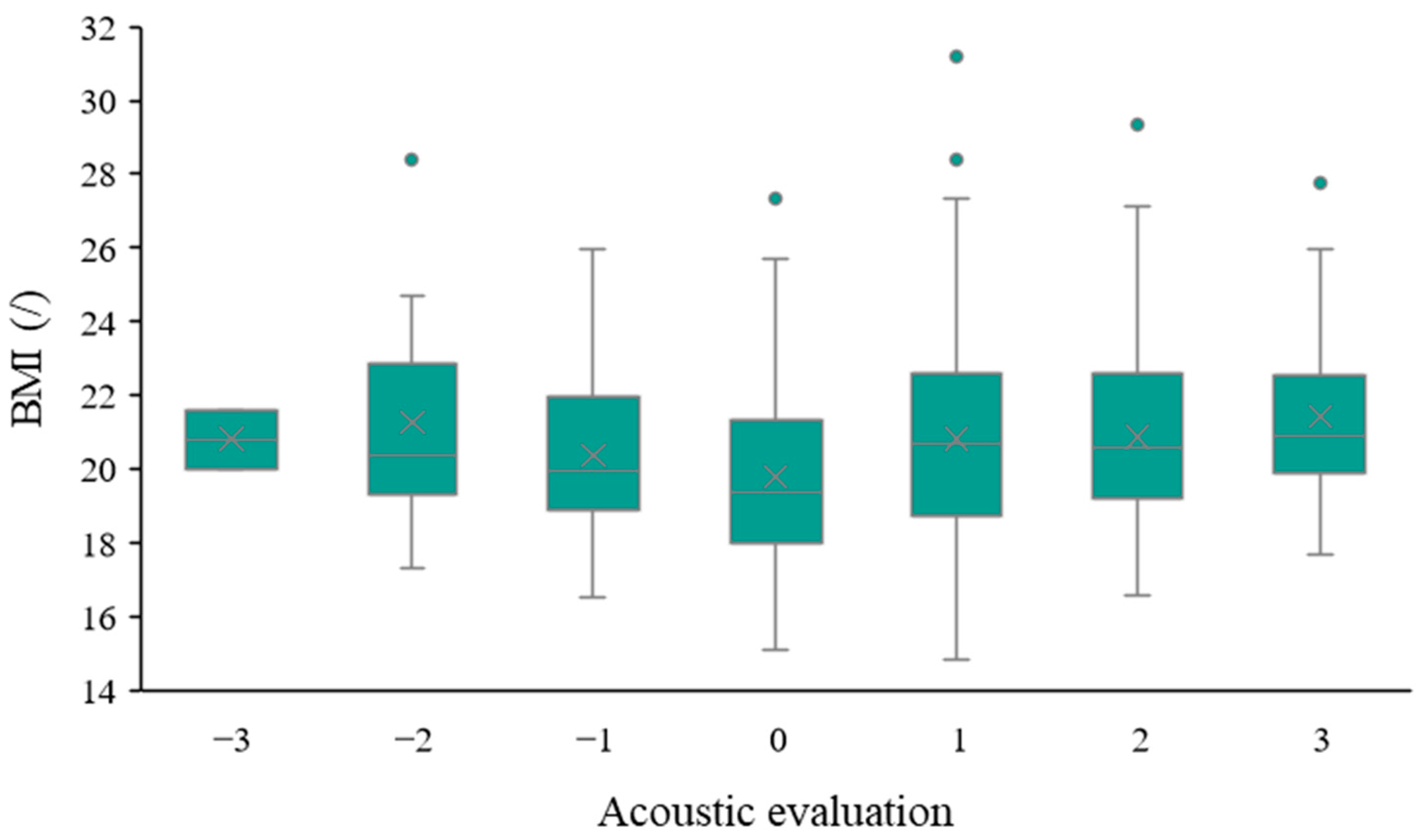
Based on the correlation analysis results shown in Table 1, it seems that acoustic satisfaction exhibits stronger associations with dose-related acoustic indicators (i.e., LAeq, LA10, and LA90), whereas acoustic acceptance demonstrates stronger relationships with room-related indicators (i.e., room type and seat location). In addition, it is worth noting that there were differences in the impact of BMI on these two parameters. Specifically, BMI showed a significant correlation with students’ acoustic satisfaction rate: the average BMI of students who were satisfied with the acoustic quality was 20.9, while it was 20.1 for those who were not satisfied with the acoustic quality. However, BMI did not correlate with students’ acoustic acceptance rate, as the average BMIs of accepting and non-accepting students were 20.5. A one-way ANOVA test was conducted to explore further the relationship between students’ BMI and their acoustic evaluations. The result indicated a significant difference in BMI between the students with different acoustic evaluations (F = 2.406, p = 0.027). As shown in Figure 10, the BMI of students who selected “0 (neutral)” was significantly lower than that of other students. One possible underlying reason is that students with lower BMI might have healthier behavior and better stress/emotion management, potentially leading to neutral evaluation. More investigations on students’ lifestyle habits and demographic factors are needed to confirm this hypothesis.
Regarding the prediction of these two parameters, the average accuracy of the six tested models for acoustic acceptance (0.72) was higher than for acoustic satisfaction (0.58). The different sizes of the training datasets might cause this. Although the original datasets were the same for the prediction of these two parameters, more cases were generated for the prediction of acoustic acceptance to address the imbalances between the positive and negative cases since the proportion of the binary classifications for acoustic acceptance was more unbalanced (85% vs. 15%) than for acoustic satisfaction (58% vs. 42%). A larger training dataset might increase the prediction accuracy. As Ng et al. [47] found, increasing the training data size significantly improved the prediction accuracy of machine learning models. However, contrasting results were reported by Bailly et al. [48], who did not identify any impact of dataset size on the model performance. Furthermore, Tsangaratos and Ilia [49] conducted a study indicating that the impact of dataset size was only significant for the LR model but not for the NB model.
The inconsistent results suggest that other factors might contribute to the different prediction accuracies for these two parameters. One potential factor is the selection of input variables. In the current study, nine variables were examined, but according to research by Hamida [50], numerous other variables could potentially influence occupants’ acoustic evaluations. These variables include heart rate, blood pressure, reverberation time, speech transmission index, floor materials, room volumes, etc. The relatively poorer prediction for acoustic satisfaction in the current study might be due to the insufficient features captured by the selected input variables. Therefore, future studies should investigate more variables influencing occupants’ acoustic satisfaction to understand the underlying factors better.
Based on the present study’s findings, it seems that acoustic acceptance is a more appropriate parameter for evaluating acoustic quality in the learning environment for the following two reasons. Firstly, the investigated machine learning models could provide a more accurate prediction of students’ acoustic acceptance in the learning spaces compared with acoustic satisfaction. Secondly, acoustic acceptance is more inclusive since it includes “neutral” opinions. Consequently, this implies that the “unacceptance” cases were relatively fewer but more significant and should be given more attention. Thus, utilizing this parameter could assist researchers and managers in identifying the spaces with more serious acoustic issues.

4.2. Comparison of Tested Machine Learning Models

Six machine learning models were trained and compared in the current study. Most of them, i.e., RF, GBM, LR, and NB, achieved an accuracy rate exceeding 70% for predicting acoustic acceptance and over 60% for acoustic satisfaction. The RF and GBM demonstrated the most favorable performance. Similar findings were reported by Boudreault et al. [51] and Luo et al. [22] in the context of modeling heat-health relationships and predicting thermal sensation, respectively. Specifically, Boudreault et al. [51] compared nine machine and deep learning models and found that RF and GBM outperformed other models in terms of prediction of heat-related mortality; Luo et al. [22] compared nine machine learning models regarding their performance in thermal sensation prediction and indicated that RF performed the best among the tested models. Two reasons might contribute to the outperformance of the GBM and RF models. Firstly, they can capture complex patterns and interactions in the data due to their ensemble nature. They can combine multiple weak learners to form a strong predictive model [52]. On the other hand, NB and LR models are relatively similar, which might limit their ability to capture complex patterns. Second, RF and GBM are more flexible and can handle diverse data distributions without any assumptions. On the other hand, LR and NB models work based on specific data distribution assumptions. To be precise, LR assumes a linear relationship between the features and the log odds [53]; NB assumes that all the features are independent of each other [53,54]. These assumptions simplify the models and increase the computational efficiency, but they also might decrease the prediction accuracies.
In terms of the performance of the SVM models, both showed poor results for predicting subjective acoustic evaluations, with SVM (Sigmoid) being particularly unsuitable. This inadequate accuracy of SVM (Sigmoid) was also identified by Wong et al. [20] in their study on predicting indoor air quality. However, in a comparison study among seven machine learning models conducted by Osisanwo et al. [55], SVM was the most accurate model in predicting diabetes. The different performances of SVM models might be related to the complex relationships between the features and the target variables. The SVM (Sigmoid) model is usually inappropriate for high-dimensional datasets [56].
Additionally, the lower accuracies observed in SVM models in the current study might also be due to the hyperparameter selection, which could significantly influence the model’s accuracy. In this study, only the default settings were tested, and no further analysis was conducted to optimize the model hyperparameters, which might impact the model’s performance. According to Wong et al. [20], modifying the hyperparameters of the SVM (Sigmoid) model could enhance the accuracy from 0.4 to 0.8. Therefore, it is plausible that a more thorough exploration and tuning of the hyperparameters could improve the SVM models’ performance in predicting students’ acoustic evaluation.

4.3. Limitations and Future Studies

There are three noteworthy limitations in this study. The first limitation pertains to the input variables and the hyperparameters used for the machine learning models. Although the survey considered three groups of indicators (occupants-related, room-related, and dose-related), only a few variables in each group were investigated, and only the default settings were applied. Numerous other variables and the impact of the hyperparameters warrant further exploration. Secondly, this study only compared six machine learning models commonly used in previous studies on indoor environmental quality. Future studies should consider exploring the performance of other models, such as deep learning, in predicting students’ acoustic evaluations. Lastly, although this study considered rooms of varying types and sizes, all were located within a single educational building. This setting may limit the broader implications of the current results. Therefore, future studies are encouraged to evaluate the performance of these models in other educational buildings as well. Furthermore, to better serve a broader range of occupants, including students, teachers, staff, and facility managers, in understanding the acoustic quality of their learning and working spaces, an easy-to-use device or application could be developed based on the machine learning model established in this study.

5. Conclusions

This study examined the acoustic quality of four rooms in a university library, including the collection of objective and subjective variables. A series of correlation analyses identified variables associated with acoustic evaluation as predictors for students’ acoustic acceptance (from neutral to totally satisfied) and acoustic satisfaction (from slightly satisfied to totally satisfied). Using these predictors as inputs, six machine learning models, i.e., Support Vector Machine–Radial Basis Function (SVM (RBF)), SVM (Sigmoid), Gradient Boosting Machine (GBM), Logistic Regression (LR), Random Forest (RF), and Naïve Bayes (NB), were established to predict students’ acoustic acceptance and acoustic satisfaction. By analyzing the results and comparing the performance of these models, the following conclusions can be drawn:
  • Personal factors (e.g., age, gender, BMI, and current feeling) significantly impact students’ acoustic evaluations. These personal factors should be considered as essential variables in future acoustic investigations.
  • The combination of age, gender, feeling, room type, seat location, and LAeq was used as input variables to predict acoustic acceptance, while the combination of age, feeling, BMI, and LAeq was applied to predict acoustic satisfaction.
  • Acoustic acceptance is more tolerant than acoustic satisfaction, as 85% of students accepted the acoustic quality in the investigated environment, while only 58% were satisfied. Moreover, the prediction accuracy of acoustic acceptance (0.72) was higher than that of acoustic satisfaction (0.58). Thus, it is recommended that future acoustic investigations prioritize acoustic acceptance as the target parameter.
  • RF and GBM models best predicted both acoustic acceptance and acoustic satisfaction, while SVM models performed the poorest, especially the SVM (Sigmoid).
This study demonstrated the feasibility of employing machine learning techniques to predict occupants’ acoustic evaluations in learning environments. This approach should be applied in future acoustic studies to avoid time-consuming and labor-intensive questionnaire surveys. However, given the limited variables and machine learning models examined in this study, there might be a more accurate prediction model that needs to be explored. Therefore, future research is suggested to conduct a broader investigation, including a more comprehensive range of variables and models, to improve the accuracy of forecasting students’ acoustic evaluations within the learning environment. Additionally, exploration of different types of learning environments, such as classrooms and lecture halls, is recommended to investigate the generalizability of these findings.

Author Contributions

Conceptualization, D.Z., L.-T.W., M.M. and K.-W.M.; methodology, L.-T.W., M.M. and D.Z.; formal analysis, D.Z.; resources, L.-T.W. and K.-W.M.; data curation, D.Z.; writing—original draft preparation, D.Z.; writing—review and editing, L.-T.W., M.M. and K.-W.M.; visualization, D.Z.; supervision, L.-T.W., M.M. and K.-W.M.; project administration L.-T.W. and K.-W.M.; funding acquisition, L.-T.W. and K.-W.M. All authors have read and agreed to the published version of the manuscript.

Funding

This research was funded by the General Research Fund, Research Grants Council of the Hong Kong Special Administrative Region, China (Project no. 15217221, PoyU P0037773/Q86B) and partially supported by the PolyU internal funds (P0040864 and P0043831).

Data Availability Statement

The data presented in this study are available on request from the corresponding author due to confidentiality and privacy concerns regarding the participants’ personal information.

Conflicts of Interest

The authors declare no conflicts of interest.

References

  1. Mealings, K. A Scoping Review of the Effects of Classroom Acoustic Conditions on Primary School Children’s Physical Health. Acoust. Aust. 2022, 50, 373–381. [Google Scholar] [CrossRef]
  2. Mealings, K. A scoping review of the effects of classroom acoustic conditions on primary school children’s mental wellbeing. Build. Acoust. 2022, 29, 529–542. [Google Scholar] [CrossRef]
  3. Wålinder, R.; Gunnarsson, K.; Runeson, R.; Smedje, G. Physiological and Psychological Stress Reactions in Relation to Classroom Noise. Scand. J. Work Environ. Health. 2007, 33, 260–266. [Google Scholar] [CrossRef] [PubMed]
  4. Klatte, M.; Hellbrück, J.; Seidel, J.; Leistner, P. Effects of Classroom Acoustics on Performance and Well-Being in Elementary School Children: A Field Study. Environ. Behav. 2010, 42, 659–692. [Google Scholar] [CrossRef]
  5. Polewczyk, I.; Jarosz, M. Teachers’ and students’ assessment of the influence of school rooms acoustic treatment on their performance and wellbeing. Arch. Acoust. 2020, 45, 401–417. [Google Scholar] [CrossRef]
  6. Astolfi, A.; Puglisi, G.E.; Murgia, S.; Minelli, G.; Pellerey, F.; Prato, A.; Sacco, T. Influence of Classroom Acoustics on Noise Disturbance and Well-Being for First Graders. Front. Psychol. 2019, 10, 2736. [Google Scholar] [CrossRef] [PubMed]
  7. Dohmen, M.; Braat-Eggen, E.; Kemperman, A.; Hornikx, M. The Effects of Noise on Cognitive Performance and Helplessness in Childhood: A Review. Int. J. Environ. Res. Public Health 2023, 20, 288. [Google Scholar] [CrossRef] [PubMed]
  8. Mealings, K. A Scoping Review of the Effect of Classroom Acoustic Conditions on Primary School Children’s Numeracy Performance and Listening Comprehension. Acoust. Aust. 2023, 51, 129–158. [Google Scholar] [CrossRef]
  9. Klatte, M.; Lachmann, T.; Meis, M. Effects of noise and reverberation on speech perception and listening comprehension of children and adults in a classroom-like setting. Noise Health 2010, 12, 270–282. [Google Scholar] [CrossRef]
  10. Prodi, N.; Visentin, C.; Borella, E.; Mammarella, I.C.; Di Domenico, A. Using speech comprehension to qualify communication in classrooms: Influence of listening condition, task complexity and students’ age and linguistic abilities. Appl. Acoust. 2021, 182, 108239. [Google Scholar] [CrossRef]
  11. Brännström, K.J.; Rudner, M.; Carlie, J.; Sahlén, B.; Gulz, A.; Andersson, K.; Johansson, R. Listening effort and fatigue in native and non-native primary school children. J. Exp. Child. Psychol. 2021, 210, 105203. [Google Scholar] [CrossRef] [PubMed]
  12. Mealings, K. Classroom acoustics and cognition: A review of the effects of noise and reverberation on primary school children’s attention and memory. Build. Acoust. 2022, 29, 401–431. [Google Scholar] [CrossRef]
  13. Masullo, M.; Ruggiero, G.; Fernandez, D.A.; Iachini, T.; Maffei, L. Effects of urban noise variability on cognitive abilities in indoor spaces: Gender differences. Noise Vib. Worldw. 2021, 52, 313–322. [Google Scholar] [CrossRef]
  14. Sarantopoulos, G.; Lykoudis, S.; Kassomenos, P. Noise levels in primary schools of medium sized city in Greece. Sci. Total Environ. 2014, 482–483, 493–500. [Google Scholar] [CrossRef] [PubMed]
  15. Kanu, M.O.; Joseph, G.W.; Targema, T.V.; Andenyangnde, D.; Mohammed, I.D. On the Noise Levels in Nursery, Primary and Secondary Schools in Jalingo, Taraba State: Are they in Conformity with the Standards? Present Environ. Sustain. Dev. 2022, 2, 95–111. [Google Scholar] [CrossRef]
  16. Tahsildoost, M.; Zomorodian, Z.S. Indoor environment quality assessment in classrooms: An integrated approach. J. Build. Phys. 2018, 42, 336–362. [Google Scholar] [CrossRef]
  17. Yang, D.; Mak, C.M. Relationships between indoor environmental quality and environmental factors in university classrooms. Build. Environ. 2020, 186, 107331. [Google Scholar] [CrossRef]
  18. Cao, B.; Ouyang, Q.; Zhu, Y.; Huang, L.; Hu, H.; Deng, G. Development of a multivariate regression model for overall satisfaction in public buildings based on field studies in Beijing and Shanghai. Build. Environ. 2012, 47, 394–399. [Google Scholar] [CrossRef]
  19. Wong, L.T.; Mui, K.W.; Hui, P.S. A multivariate-logistic model for acceptance of indoor environmental quality (IEQ) in offices. Build. Environ. 2008, 43, 1–6. [Google Scholar] [CrossRef]
  20. Wong, L.T.; Mui, K.W.; Tsang, T.W. Updating Indoor Air Quality (IAQ) Assessment Screening Levels with Machine Learning Models. Int. J. Environ. Res. Public Health 2022, 19, 5724. [Google Scholar] [CrossRef]
  21. Zhang, W.; Wu, Y.; Calautit, J.K. A review on occupancy prediction through machine learning for enhancing energy efficiency, air quality and thermal comfort in the built environment. Renew. Sustain. Energy Rev. 2022, 167, 112704. [Google Scholar] [CrossRef]
  22. Luo, M.; Xie, J.; Yan, Y.; Ke, Z.; Yu, P.; Wang, Z.; Zhang, J. Comparing machine learning algorithms in predicting thermal sensation using ASHRAE Comfort Database II. Energy Build. 2020, 210, 109776. [Google Scholar] [CrossRef]
  23. Chai, Q.; Wang, H.; Zhai, Y.; Yang, L. Using machine learning algorithms to predict occupants’ thermal comfort in naturally ventilated residential buildings. Energy Build. 2020, 217, 109937. [Google Scholar] [CrossRef]
  24. Huang, H.B.; Huang, X.R.; Li, R.X.; Lim, T.C.; Ding, W.P. Sound quality prediction of vehicle interior noise using deep belief networks. Appl. Acoust. 2016, 113, 149–161. [Google Scholar] [CrossRef]
  25. Wang, R.; Yao, D.; Zhang, J.; Xiao, X.; Xu, Z. Identification of Key Factors Influencing Sound Insulation Performance of High-Speed Train Composite Floor Based on Machine Learning. Acoustics 2024, 6, 1–17. [Google Scholar] [CrossRef]
  26. Zhang, E.; Peng, Z.; Zhuo, J. A case study on improving electric bus interior sound quality based on sensitivity analysis of psycho-acoustics parameters. Noise Vib. Worldw. 2023, 54, 460–468. [Google Scholar] [CrossRef]
  27. Yeh, C.Y.; Tsay, Y.S. Using machine learning to predict indoor acoustic indicators of multi-functional activity centers. Appl. Sci. 2021, 11, 5641. [Google Scholar] [CrossRef]
  28. Bonet-Solà, D.; Vidaña-Vila, E.; Alsina-Pagès, R.M. Prediction of the acoustic comfort of a dwelling based on automatic sound event detection. Noise Mapp. 2023, 10, 20220177. [Google Scholar] [CrossRef]
  29. Puyana-Romero, V.; Díaz-Márquez, A.M.; Ciaburro, G.; Hernández-Molina, R. The Acoustic Environment and University Students’ Satisfaction with the Online Education Method during the COVID-19 Lockdown. Int. J. Environ. Res. Public Health 2023, 20, 709. [Google Scholar] [CrossRef]
  30. Puyana-Romero, V.; Larrea-Álvarez, C.M.; Díaz-Márquez, A.M.; Hernández-Molina, R.; Ciaburro, G. Developing a Model to Predict Self-Reported Student Performance during Online Education Based on the Acoustic Environment. Sustainability 2024, 16, 4411. [Google Scholar] [CrossRef]
  31. The Chartered Institution of Building Services Engineers. CIBSE TM68: Monitoring Indoor Environment Quality; The Chartered Institution of Building Services Engineers: London, UK, 2022. [Google Scholar]
  32. Aryal, A.; Becerik-Gerber, B. Thermal comfort modeling when personalized comfort systems are in use: Comparison of sensing and learning methods. Build. Environ. 2020, 185, 107316. [Google Scholar] [CrossRef]
  33. Hagberg, K.G. Evaluating field measurements of impact sound. Build. Acoust. 2010, 17, 105–128. [Google Scholar] [CrossRef]
  34. Karmann, C.; Schiavon, S.; Arens, E. Percentage of Commercial Buildings Showing at Least 80% Occupant Satisfied with Their Thermal Comfort. Available online: www.escholarship.org/uc/item/89m0z34x (accessed on 25 May 2024).
  35. Tsang, T.W.; Mui, K.W.; Wong, L.T.; Yu, W. Bayesian updates for indoor environmental quality (IEQ) acceptance model for residential buildings. Intell. Build. Int. 2021, 13, 17–32. [Google Scholar] [CrossRef]
  36. Ghazal, S.; Aldowah, H.; Umar, I.N. The relationship between acceptance and satisfaction of learning environment system usage in a balanced learning environment. J. Fundam. Appl. Sci. 2018, 10, 858–870. [Google Scholar] [CrossRef]
  37. NSW Environment Protection Authority, Noise Guide for Local Government. NSW Environment Protection Authority. 2023. Available online: https://www.epa.nsw.gov.au/your-environment/noise/regulating-noise/noise-guide-local-government (accessed on 25 May 2024).
  38. Chawla, N.V.; Bowyer, K.W.; Hall, L.O.; Kegelmeyer, W.P. SMOTE: Synthetic Minority Over-Sampling Technique. Artif. Intell. Res. 2002, 16, 321–357. [Google Scholar] [CrossRef]
  39. Akın, P. A new hybrid approach based on genetic algorithm and support vector machine methods for hyperparameter optimization in synthetic minority over-sampling technique (SMOTE). AIMS Math. 2023, 8, 9400–9415. [Google Scholar] [CrossRef]
  40. Satriaji, W.; Kusumaningrum, R. Effect of Synthetic Minority Oversampling Technique (SMOTE), Feature Representation, and Classification Algorithm on Imbalanced Sentiment Analysis. In Proceedings of the 2nd International Conference on Informatics and Computational Sciences (ICICoS), Semarang, Indonesia, 30–31 October 2018; pp. 1–5. [Google Scholar]
  41. Ghosh, S.; Dasgupta, A.; Swetapadma, A. A study on support vector machine based linear and non-linear pattern classification. In Proceedings of the 2019 International Conference on Intelligent Sustainable Systems (ICISS), Palladam, India, 21–22 February 2019; pp. 24–28. [Google Scholar]
  42. Ayyadevara, V.K. Gradient Boosting Machine. In Pro Machine Learning Algorithms, 1st ed.; Apress: Berkeley, CA, USA, 2018; pp. 117–134. [Google Scholar]
  43. Ayyadevara, V.K. Logistic Regression. In Pro Machine Learning Algorithms: A Hands-On Approach to Implementing Algorithms in Python and R, 1st ed.; Apress: Berkeley, CA, USA, 2018; pp. 49–69. [Google Scholar] [CrossRef]
  44. Ayyadevara, V.K. Random Forest. In Pro Machine Learning Algorithms, 1st ed.; Apress: Berkeley, CA, USA, 2018; pp. 105–116. [Google Scholar]
  45. Chen, S.; Webb, G.I.; Liu, L.; Ma, X. A novel selective naïve Bayes algorithm. Knowl.-Based Syst. 2020, 192, 105361. [Google Scholar] [CrossRef]
  46. Tang, S.K. Performance of noise indices in air-conditioned landscaped office buildings. J. Acoust. Soc. Am. 1997, 102, 1657–1663. [Google Scholar] [CrossRef] [PubMed]
  47. Ng, W.; Minasny, B.; de Sousa Mendes, W.; Demattê, J.A.M. The influence of training sample size on the accuracy of deep learning models for the prediction of soil properties with near-infrared spectroscopy data. SOIL 2020, 6, 565–578. [Google Scholar] [CrossRef]
  48. Bailly, A.; Blanc, C.; Francis, É.; Guillotin, T.; Jamal, F.; Wakim, B.; Roy, P. Effects of dataset size and interactions on the prediction performance of logistic regression and deep learning models. Comput. Methods Programs Biomed. 2022, 213, 106504. [Google Scholar] [CrossRef]
  49. Tsangaratos, P.; Ilia, I. Comparison of a logistic regression and Naïve Bayes classifier in landslide susceptibility assessments: The influence of models complexity and training dataset size. Catena 2016, 145, 164–179. [Google Scholar] [CrossRef]
  50. Hamida, A.; Zhang, D.; Ortiz, M.A.; Bluyssen, P.M. Indicators and methods for assessing acoustical preferences and needs of students in educational buildings: A review. Appl. Acoust. 2023, 202, 109187. [Google Scholar] [CrossRef]
  51. Boudreault, J.; Campagna, C.; Chebana, F. Machine and deep learning for modelling heat-health relationships. Sci. Total Environ. 2023, 892, 164660. [Google Scholar] [CrossRef] [PubMed]
  52. Ayyadevara, V.K. Pro Machine Learning Algorithms: A Hands-On Approach to Implementing Algorithms in Python and R; Apress Media LLC: Berkeley, CA, USA, 2018. [Google Scholar] [CrossRef]
  53. Steyerberg, E.W. Clinical Prediction Models A Practical Approach to Development, Validation, and Updating, 2nd ed.; Springer: Chem, Switzerland, 2019. [Google Scholar]
  54. Kelly, A.; Johnson, M.A. Investigating the statistical assumptions of naïve bayes classifiers. In Proceedings of the 2021 55th Annual Conference on Information Sciences and Systems, CISS 2021, Baltimore, MD, USA, 24–26 March 2021; Institute of Electrical and Electronics Engineers Inc.: New York, NY, USA, 2021. [Google Scholar] [CrossRef]
  55. Osisanwo, F.Y.; Akinsola, J.E.T.; Awodele, O.; Hinmikaiye, J.O.; Olakanmi, O.; Akinjobi, J. Supervised Machine Learning Algorithms: Classification and Comparison. Int. J. Comput. Trends Technol. 2017, 48, 128–138. [Google Scholar] [CrossRef]
  56. Kar, A.; Nath, N.; Kemprai, U.; Aman. Performance Analysis of Support Vector Machine (SVM) on Challenging Datasets for Forest Fire Detection. Int. J. Commun. Netw. Syst. Sci. 2024, 17, 11–29. [Google Scholar] [CrossRef]
Figure 1. Overall research flowchart.
Acoustics 06 00037 g001
Figure 2. The measurement device and location.
Acoustics 06 00037 g002
Figure 3. Definition of “acoustic satisfaction” and “acoustic acceptance” in the current study.
Acoustics 06 00037 g003
Figure 4. Model development process.
Acoustics 06 00037 g004
Figure 5. Participants’ acoustic evaluations.
Acoustics 06 00037 g005
Figure 6. Acoustic acceptance prediction accuracies of the tested models. Note: AA in the figures represents acoustic acceptance.
Acoustics 06 00037 g006
Figure 7. Evaluation of the tested models for acoustic acceptance prediction.
Acoustics 06 00037 g007
Figure 8. Acoustic satisfaction prediction accuracies of the tested models. Note: AS in the figures represents acoustic satisfaction.
Acoustics 06 00037 g008
Figure 9. Evaluation of the tested models for acoustic satisfaction prediction.
Acoustics 06 00037 g009
Figure 10. Relationship between students’ BMI and their acoustic evaluations. Note: the bottom of the box representing the 1st quartile (25th percentile) of the data; the top of the box representing the 3rd quartile (75th percentile) of the data; the line inside the box indicating the median (2nd quartile) of the data. The “×” symbol inside the box represents the mean value of the data; the whiskers outside the box represent the minimum and maximum values of the data; the points outside the whiskers represent outliers.
Acoustics 06 00037 g010
Table 1. Relationships between the potential predictors and the acoustic acceptance/satisfaction.
Variables N = 398Acoustic AcceptanceAcoustic Satisfaction
Occupant-related indicators
Age21.3 (3.5)t = −3.115 (p = 0.002)t = −2.224 (p = 0.027)
GenderFemale190 (48%)Χ2 = 3.324 (p = 0.068)Χ2 = 1.611 (p = 0.204)
Male208 (52%)
FeelingGood295 (74%)Χ2 = 4.775 (p = 0.092)Χ2 = 9.831 (p = 0.007)
Neutral95 (24%)
Bad8 (2%)
BMI20.5 (2.6)t = −0.033 (p = 0.974)t = 3.142 (p = 0.002)
Room-related indicators
Room typeGroup 228 (57%)Χ2 = 8.642 (p = 0.003)Χ2 = 0.269 (p = 0.604)
Self170 (43%)
Seat locationMiddle213 (54%)Χ2 = 12.381 (p = 0.002)Χ2 = 2.055 (p = 0.358)
Others185 (46%)
Dose-related indicators
LAeq50.1 (6.2)t = −1.033 (p = 0.302)t = −2.502 (p = 0.013)
LA9049.1 (6.7)t = −0.806 (p = 0.421)t = −2.356 (p = 0.019)
LA1051.1 (6.0)t = −1.038 (p = 0.304)t = −2.483 (p = 0.013)
Note: independent t-tests were conducted to check the impact of age, BMI, LAeq, LA10, and LA90 on students’ acoustic acceptance/satisfaction; Chi-square tests were conducted to check the impact of feeling, room type, and seat location on students’ acoustic acceptance/satisfaction. p-values less than 0.1 were marked in bold.
Table 2. Correlations between the predicted and collected acoustic acceptance.
Models PredictedAccepted
N (%)
Unaccepted
n (%)
p *
Collected
SVM (Sigmoid)Accepted 52 (37.7%)26 (18.8%)0.199
Unaccepted 46 (33.3%)14 (10.1%)
SVM (RBF)Accepted 53 (38.4%)25 (18.1%)<0.001
Unaccepted 22 (15.9%)38 (27.5%)
NBAccepted 60 (43.5%)18 (13.0%)<0.001
Unaccepted 16 (11.6%)44 (31.9%)
LRAccepted 63 (43.5%)15 (10.9%)<0.001
Unaccepted 15 (10.9%)45 (32.6%)
GBMAccepted 67 (48.6%)11 (8.0%)<0.001
Unaccepted 13 (9.4%)47 (34.1%)
RFAccepted 69 (50.0%)9 (6.5%)<0.001
Unaccepted 14 (10.1%)46 (33.3%)
Note: * p-values were obtained from the Chi-square tests, and p-values less than 0.05 were marked in bold.
Table 3. Correlations between the predicted and collected acoustic satisfaction.
Models PredictedSatisfied n (%)Dissatisfied n (%)p *
Collected
SVM (Sigmoid)Satisfied 51 (54.3%)0 (0%)/
Dissatisfied 43 (45.7%)0 (0%)
SVM (RBF)Satisfied 24 (25.5%)19 (20.2%)0.221
Dissatisfied 22 (23.4%)29 (30.9%)
NBSatisfied 32 (34.0%)11 (11.7%)0.002
Dissatisfied 22 (23.4%)29 (30.9%)
LRSatisfied 25 (26.6%)18 (19.1%)0.208
Dissatisfied 23 (24.5%)28 (29.8%)
GBMSatisfied 28 (29.8%)15 (16.0%)0.001
Dissatisfied 16 (17.0%)35 (37.2%)
RFSatisfied 30 (31.9%)13 (13.8%)<0.001
Dissatisfied 18 (19.1%)33 (35.1%)
Note: * p-values were obtained from Chi-square tests, and p-values less than 0.05 were marked in bold.
Disclaimer/Publisher’s Note: The statements, opinions and data contained in all publications are solely those of the individual author(s) and contributor(s) and not of MDPI and/or the editor(s). MDPI and/or the editor(s) disclaim responsibility for any injury to people or property resulting from any ideas, methods, instructions or products referred to in the content.