A Stable IIR Filter Design Approach for High-Order Active Noise Control Applications

Abstract

In commercial non-adaptive active noise control (ANC) applications, an IIR filter structure is often used to reduce real-time computations. On the contrary, an FIR filter structure is usually preferred in the filter design phase because the FIR filter design formulation can be convex and is simple to solve. To combine the benefits of both FIR and IIR filter structures, one common approach in ANC applications is to use an IIR filter structure to fit a pre-designed FIR filter. However, to ensure stability, most of the common IIR filter fitting approaches involve the computation and relocation of poles which can be difficult for high-order cases. In this current work, a stable IIR filter design approach that does not need the computation and relocation of poles is improved to be applicable in ANC applications. The results demonstrate that the proposed method can achieve better fitting accuracy and steady-state noise control performance in high-order non-adaptive applications when the pre-designed noise control FIR filter is fitted. Besides fitting the noise control filter, the proposed method can also be used to fit the secondary path and acoustic feedback path to reduce the required real-time computations if adaptive controllers are applied.

1. Introduction

Active noise control (ANC) techniques have been implemented in a wide range of applications in the past decades, such as headrests [1], automobiles [2], motorcycle helmets [3], air-conditioners [4,5], ventilation windows [6], etc. In most of these practical applications, finite impulse response (FIR) filters were used because of their simplicity and stability in real-time implementation [7]. Besides the real-time implementation phase, the use of a FIR filter structure can be more beneficial in the design phase because the filter response will be a linear function of the FIR filter coefficients to be designed and it simplifies the filter design problem formulation. Moreover, various practical constraints shall be considered when designing the ANC filter coefficients in many commercial ANC applications, e.g., headphones [8], vehicles [2], and air-conditioners [4,5]. The constrained filter design problem can be formulated to be a convex problem if an FIR filter structure is used in the control filter and the global optimal filter coefficients can be obtained [2,4].

However, compared with the infinite impulse response (IIR) filter, the FIR filter usually requires a longer filter length, thus, a higher real-time computational power. In many commercial ANC applications, a high sampling rate may be chosen for multiple reasons [9], e.g., to reduce the electronic delay to improve the noise control performance [10], to achieve a wider frequency band [11], to be compatible with the sampling rate in audio applications, etc. The use of a high sampling rate in ANC systems significantly increases the required order of control filters if an FIR filter structure is used [9,11]. Thus, an IIR filter structure is preferred in high-sampling cases to reduce the real-time computations at the sacrifice of simplicity in the filter design phase.

One common approach in ANC applications to combine the benefits of both FIR and IIR filter structures is to use an IIR filter structure to fit pre-designed FIR filter coefficients (or the desired frequency responses). Thus, the desired time-domain filter coefficients or frequency-domain responses can be designed first using the FIR filter structure to simplify computation in the filter design phase. Then, an IIR filter is fitted from the desired time-domain coefficients or the frequency-domain responses. The most challenging part of using this approach is that the designed IIR filter should be stable. Many traditional IIR filter fitting methods cannot ensure stability directly, such as the prony’s method [12], stmcb method [13,14], the least-square approximation in the frequency domain using equation error method [15], or the damped Gauss–Newton method [16]. To ensure stability, most of the methods compute the poles and map the unstable poles to the inside of the unit circle in the z-transform domain at each iteration. However, for high-order cases, numerically computing the poles (i.e., computing the roots of a high-order polynomial) can be difficult [17,18], which makes many traditional stable IIR filter approximation approaches not suitable to be used in high sampling rate ANC applications. Thus, a stable IIR approximation approach for high sampling rate ANC applications should be developed.

In this paper, to fit a stable IIR filter for non-adaptive ANC applications, the IIR filter approximation method proposed by Brandenstein and Unbehauen [19,20] is adopted. Improvements are proposed based on their method to make it applicable in ANC applications. A non-adaptive ANC system installed on a commercial earphone prototype is used to investigate the performance of the proposed method. The result shows that the proposed improved IIR filter approximation method can achieve better fitting accuracy and noise control performance compared with the traditional IIR fitting approach. Besides fitting the noise control filter, the proposed method can also be applied to the fitting of secondary paths and acoustic feedback paths to further reduce the real-time computations if adaptive controllers are applied.

2. Methods

In this section, the commonly used traditional stable IIR filter fitting approach is first reviewed. Then, the method proposed by Brandenstein and Unbehauen is reviewed and the proposed improvements based on their method are explained. Only FIR and IIR filters with real-valued time-domain coefficients are considered in this article.

Let the transfer function of the FIR filter that needs to be approximated be

$$F\left(z\right)=\sum _{n=0}^L{f}_n{z}^{-n}.$$

(1)

The transfer function of a causal and stable IIR filter is expressed as

$$H\left(z\right)=\frac{P\left(z\right)}{Q\left(z\right)},$$

(2)

where, the numerator polynomial $P\left(z\right)$ is

$$P\left(z\right)=\sum _{\mu =0}^M{p}_{\mu }{z}^{-\mu },$$

(3)

and the denominator polynomial $Q\left(z\right)$ is

$$Q\left(z\right)=1+\sum _{\nu =1}^N{q}_{\nu }{z}^{-\nu }.$$

(4)

The objective of fitting an FIR filter using an IIR filter structure is to minimize the approximation error

$$E={\left(\frac{1}{2\pi }{\int }_{-\pi }^{\pi }W\left(e^{j\mathrm{\Omega }}\right){\left|F\left(e^{j\mathrm{\Omega }}\right)-H\left(e^{j\mathrm{\Omega }}\right)\right|}^{2}d\mathrm{\Omega }\right)}^{\frac{1}{2}},$$

(5)

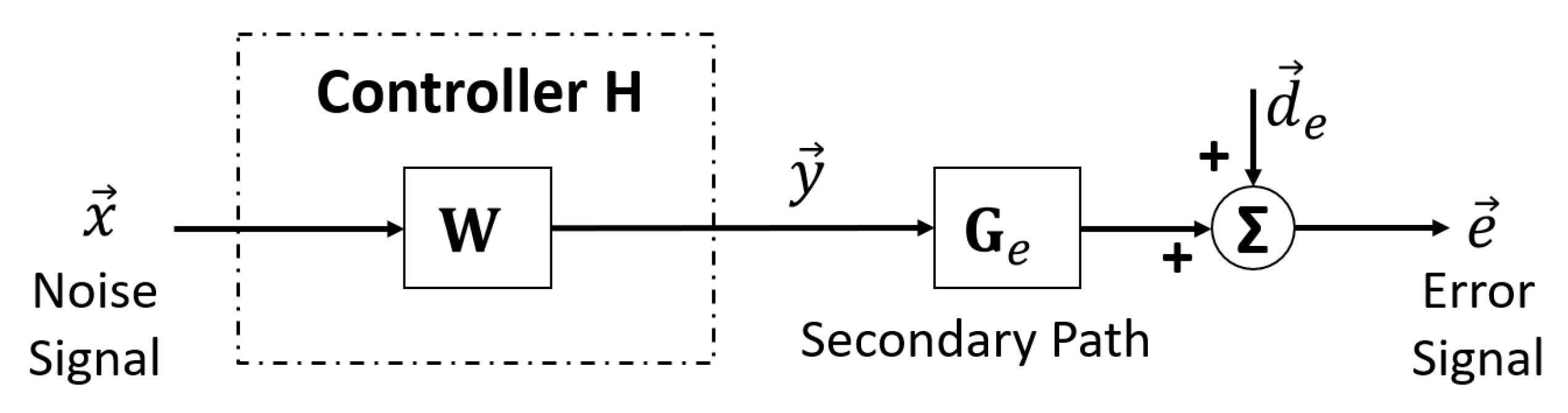
with respect to $p_{\mu }$ ($\mu$ = 0, 1, ⋯, M) and $q_{\nu }$ ($\nu$ = 1, 2, ⋯, N), where $W\left(e^{j\mathrm{\Omega }}\right)$ denotes the weighting function and $W\left(e^{-j\mathrm{\Omega }}\right)=W\left(e^{j\mathrm{\Omega }}\right)$ if the fitted FIR filter has only real coefficients.

2.1. Review of Traditional Stable IIR Filter Fitting Method

One commonly used traditional stable IIR filter fitting method is reviewed here. For simplicity, this approach is referred to as the “traditional method” in this article.

For this traditional method, instead of the objective function value E used in Equation (5), a discrete form of fitting error is formulated for numerical computation:

$$E_s=\sum _{i=0}^{N_f}W\left(e^{j{\mathrm{\Omega }}_i}\right){\left|F\left(e^{j{\mathrm{\Omega }}_i}\right)-H\left(e^{j{\mathrm{\Omega }}_i}\right)\right|}^2,$$

(6)

where ${\mathrm{\Omega }}_i$ is the i-th sampled frequency, and $N_f$ is the total number of considered discretized frequency points. If the total number of frequencies is chosen to be sufficiently large, then minimizing $E_s$ in Equation (6) can lead to approximately the same optimal filter coefficients compared with minimizing E in Equation (5). To find the optimal filter coefficients that minimize $E_s$ in Equation (6), some iterative search algorithms can be implemented, e.g., the damped Gauss–Newton method [16]. The initial point for the iterative search algorithms can be chosen using the optimal coefficients solved by minimizing the equation error formulation [15]:

$$E_l=\sum _{i=0}^{N_f}W\left(e^{j{\mathrm{\Omega }}_i}\right){\left|F\left(e^{j{\mathrm{\Omega }}_i}\right)Q\left(e^{j{\mathrm{\Omega }}_i}\right)-P\left(e^{j{\mathrm{\Omega }}_i}\right)\right|}^2.$$

(7)

Better fitting accuracy may be achieved by changing the limit of the integral in Equation (5), or the lower and upper bounds in summation in Equations (6) and (7) to the desired noise control range instead of the whole frequency range. However, this may lead to inaccurate fitting outside the desired frequency band and cause noise amplifications. Thus, in this presented work, the fitting procedure is still targeting the whole frequency range but a weighting function W is used to improve the fitting accuracy in the desired frequency range.

To ensure stability, at each iteration, the roots of the polynomial $Q\left(z\right)$, i.e., the poles, should be computed and checked. If some roots $z_i$ are outside the unit circle in the z-transform domain (i.e., $|z_i|>1$), they should be stabilized by replacing $z_i$ with $1/z_i^{*}$ where $z_i^{*}$ is the complex conjugate of $z_i$. This traditional method is used in many IIR filter fitting toolboxes such as the invfreqz() function in Matlab R2022b.

The challenge of using this traditional method for high-order IIR filter cases is that computing the roots of a high-order polynomial can be difficult and there is no guarantee that the traditional method can converge when the pole stabilizing process is applied.

2.2. Review of a Weighted Least-Square Approximation Method

A least-square method for approximating an FIR filter using an IIR filter structure that guarantees the fitted IIR filter is stable without mapping unstable poles inside the unit circle was proposed by Brandenstein and Unbehauen [19] and then extended to its weighted version [20]. Since no computation and mapping of poles are required, it is applicable even in cases where the IIR filter length is large [19,20]. Another advantage of their proposed method is that the optimal denominator coefficients can be fitted first. The optimal numerator coefficients can then be computed using the optimal denominator coefficients. For simplicity, their original proposed method is referred to as the “BU’s method” in this article. Their method is briefly summarized as follows (See Brandenstein and Unbehauen’s work for more details [19,20]).

A user-defined weighting function $W\left(e^{j\mathrm{\Omega }}\right)$ is usually real and positive (i.e., having zero phases). However, the phase of the weighting function $W\left(e^{j\mathrm{\Omega }}\right)$ in Equation (6) can be arbitrary as long as the magnitude satisfies the required weighting shape. Brandenstein and Unbehauen proved that if a maximum phase weighting function is used, it can make their proposed method likely to converge to the optimal solution. [19,20] Thus, assume that there is a maximum phase function $G\left(z\right)$ with order K satisfying $|G\left(e^{j\mathrm{\Omega }}\right){|}^2=W\left(e^{j\mathrm{\Omega }}\right)$. Then, a function $X\left(z\right)$ can be defined as

$$X\left(z\right)=z^{-K}{G}_{*}\left(z^{-1}\right)z^{-L}{F}_{*}\left(z^{-1}\right),$$

(8)

where $G_{*}\left(z\right)$ denotes the polynomial which is obtained from $G\left(z\right)$ by replacing each coefficient with its conjugate complex counterpart, and $F_{*}\left(z\right)$ is defined in a similar way. By using $X\left(z\right)$, starting from an initial guess $Q^0\left(z\right)=1$, the optimal coefficients in the denominator of the IIR filter $Q\left(z\right)$ can be solved iteratively [19,20]. More specifically, suppose at the k-th iteration, $X^{\left(k\right)}\left(z\right)$ is defined as

$$X^{\left(k\right)}\left(z\right)=\frac{X\left(z\right)}{Q^{(k-1)}\left(z\right)},$$

(9)

where $Q^{(k-1)}\left(z\right)$ is the $Q\left(z\right)$ obtained in the $(k-1)$-th iteration. In practice, Equation (9) means the $X^{\left(k\right)}$ can be obtained by filtering the coefficients of $X\left(z\right)$ using an IIR filter with 1 in the numerator and $Q^{(k-1)}\left(z\right)$ in the denominator. Then, $Q^{\left(k\right)}\left(z\right)$ can be obtained by solving the set of equations

$${\mathbf{A}}^{\left(k\right)}{\overrightarrow{q}}^{\left(k\right)}={\overrightarrow{b}}^{\left(k\right)},$$

(10)

in a least-square sense, i.e., ${\overrightarrow{q}}^{\left(k\right)}={({{\mathbf{A}}^{\left(k\right)}}^{\mathrm{T}}{\mathbf{A}}^{\left(k\right)})}^{-1}({{\mathbf{A}}^{\left(k\right)}}^{\mathrm{T}}{\overrightarrow{b}}^{\left(k\right)})$, where

$${\mathbf{A}}^{\left(k\right)}=\left[\begin{array}{cccc}{x}^{\left(k\right)}\left(0\right)& 0& \cdots & 0\\ x^{\left(k\right)}\left(1\right)& x^{\left(k\right)}\left(0\right)& \cdots & 0\\ ⋮& ⋮& \ddots & 0\\ x^{\left(k\right)}(N-1)& x^{\left(k\right)}(N-1)& \cdots & x^{\left(k\right)}\left(0\right)\\ x^{\left(k\right)}(L+N-M-1)& x^{\left(k\right)}(L+N-M-2)& \cdots & x^{\left(k\right)}(L-M)\end{array}\right],$$

(11)

$${\overrightarrow{b}}^{\left(k\right)}=-{\left[\begin{array}{cccccc}0& \cdots & 0& x^{\left(k\right)}\left(0\right)& \cdots & x^{\left(k\right)}(L-M-1)\end{array}\right]}^{\mathrm{T}},$$

(12)

and $x^{\left(k\right)}\left(n\right)$ is the sequence obtained by the inverse z-transform of $X^{\left(k\right)}\left(z\right)$. The solved ${\overrightarrow{q}}^{\left(k\right)}$ consists of the coefficients of $Q^{\left(k\right)}\left(z\right)$,

$${\overrightarrow{q}}^{\left(k\right)}={\left[\begin{array}{cccc}{q}_N^{\left(k\right)}& q_{N-1}^{\left(k\right)}& \cdots & q_1^{\left(k\right)}\end{array}\right]}^{\mathrm{T}}.$$

(13)

The approximation error norm at k-th iteration is defined as

$$E^{\left(k\right)}=\sum _{n=0}^{L+N-M-1}{u}^{\left(k\right)}{\left(n\right)}^2,$$

(14)

where $u^{\left(k\right)}\left(n\right)$ is the sequence obtained by the inverse z-transform of $U^{\left(k\right)}\left(z\right)$ and

$$U^{\left(k\right)}\left(z\right)=z^{-N}{Q}^{\left(k\right)}\left(z^{-1}\right)X^{\left(k\right)}\left(z\right).$$

(15)

After the optimal denominator coefficients, $Q\left(z\right)$ is obtained, and the optimal numerator coefficients $P\left(z\right)$ can be obtained by solving the $M+1$ linear equations

$$\sum _{\mu =0}^{M}c(\lambda -\mu )p_{\mu }=d\left(\lambda \right),$$

(16)

for $\lambda$ = 0, 1, …, M, where

$$c\left(n\right)=\frac{1}{2\pi }{\int }_{-\pi }^{\pi }\frac{W\left(e^{j\mathrm{\Omega }}\right)}{|Q\left(e^{j\mathrm{\Omega }}\right){|}^2}{e}^{jn\mathrm{\Omega }}d\mathrm{\Omega }$$

(17)

$$d\left(n\right)=\frac{1}{2\pi }{\int }_{-\pi }^{\pi }W\left(e^{j\mathrm{\Omega }}\right)\frac{F\left(e^{j\mathrm{\Omega }}\right)}{{\left[Q\left(e^{j\mathrm{\Omega }}\right)\right]}^{*}}{e}^{jn\mathrm{\Omega }}d\mathrm{\Omega }$$

(18)

2.3. Proposed Improvements in Weighted Least-Square Approximation Method for ANC Applications

In this section, some improvements are made to the BU’s method such that it is more suitable for practical ANC applications. For simplicity, these improvements on BU’s method are referred to as the “proposed method” in this article.

When using the iteration process described in the previous section, the approximation error norm $E^{\left(k\right)}$ does not always converge to the minimum value, especially for some maximum phase FIR filters with high orders (larger than 50) [19]. Thus, instead of using the $Q^{\left(k\right)}\left(z\right)$ solved at the last iteration, Brandenstein and Unbehauen suggested trying a sufficiently large number of iterations and then choosing the one with the lowest approximation error norm [19]. In ANC applications, the order of the FIR filter is usually larger than 50. This phenomenon is more likely to happen. Since this phenomenon occurs when the matrix ${\mathbf{A}}^{\left(k\right)}$ is ill-conditioned [19], one improvement is proposed as follows. If ${{\mathbf{A}}^{\left(k\right)}}^{\mathrm{T}}{\mathbf{A}}^{\left(k\right)}$ is near singular at the current iteration, then a gradient descent is applied to continue solving $Q\left(z\right)$. More specifically, the goal of solving Equation (10) is to minimize

$$\begin{array}{cc}\hfill J\left({\overrightarrow{q}}^{\left(k\right)}\right)& =\parallel {\mathbf{A}}^{\left(k\right)}{\overrightarrow{q}}^{\left(k\right)}-{\overrightarrow{b}}^{\left(k\right)}{\parallel }_2^2\hfill \\ \hfill & ={\overrightarrow{q}}^{{\left(k\right)}^{\mathrm{T}}}{\mathbf{A}}^{{\left(k\right)}^{\mathrm{T}}}{\mathbf{A}}^{\left(k\right)}{\overrightarrow{q}}^{\left(k\right)}-2{\overrightarrow{b}}^{{\left(k\right)}^{\mathrm{T}}}{\mathbf{A}}^{\left(k\right)}{\overrightarrow{q}}^{\left(k\right)}+{\overrightarrow{b}}^{{\left(k\right)}^{\mathrm{T}}}{\overrightarrow{b}}^{\left(k\right)}.\hfill \end{array}$$

(19)

Thus, $\widehat{\overrightarrow{g}}$, an estimation of the gradient of the function $J({\overrightarrow{q}}^{\left(k\right)})$ can be obtained by using ${\overrightarrow{q}}^{(k-1)}$

$$\widehat{\overrightarrow{g}}=2{{\mathbf{A}}^{\left(k\right)}}^{\mathrm{T}}{\mathbf{A}}^{\left(k\right)}{\overrightarrow{q}}^{(k-1)}-2{{\mathbf{A}}^{\left(k\right)}}^{\mathrm{T}}{\overrightarrow{b}}^{\left(k\right)}.$$

(20)

The approximated ${\overrightarrow{q}}^{\left(k\right)}$ can then be obtained by

$${\overrightarrow{q}}^{\left(k\right)}={\overrightarrow{q}}^{(k-1)}-\alpha \widehat{\overrightarrow{g}},$$

(21)

where $\alpha >0$ is the step length such that $Q^{\left(k\right)}\left(z\right)$ is stable and can have a smaller approximation error norm compared with $Q^{\left(k\right)}(z-1)$. Repeat this process until some prescribed convergence criteria are satisfied, e.g., step length, norm of gradient, etc. Note that this proposed gradient method is implemented once in each step but if it is implemented sufficiently many times in each step and well-conditioned, it will likely approach the solution obtained using BU’s original method. The ability to use prescribed convergence criteria in the proposed gradient method can be helpful to prevent the issues caused by the large condition number.

The selection of maximum phase weighting function $G\left(z\right)$ also needs to be considered. In ANC applications, the required weighting function is usually in the form of $\left|W\right(e^{-j\mathrm{\Omega }}\left)\right|$. For simplicity, a linear-phase FIR filter with real coefficients can be easily designed to have the magnitude $\sqrt{\left|W\right(e^{-j\mathrm{\Omega }}\left)\right|}$, such that $W\left(e^{-j\mathrm{\Omega }}\right)=W\left(e^{j\mathrm{\Omega }}\right)$ is satisfied. Because of the linear phase, the coefficients of this designed filter will be symmetric such that a spectral factorization can be applied to the coefficient sequence of this FIR filter to obtain a minimum phase decomposition. After flipping the coefficients of decomposed minimum phase filter, the maximum phase counterpart $G\left(z\right)$ can be obtained.

Since the signal used in the ANC controller is usually in a discrete format, the computation of c(n) and b(n) in Equations (17) and (18) is done by FFT and IFFT after a sufficiently large zero padding.

In summary, the whole proposed process of fitting an FIR filter using an IIR filter structure is presented in Algorithms 1–3. 

Algorithm 1: Finding an appropriate weighting function

Input: desired weighting curve $\left|W\right(e^{j\mathrm{\Omega }}\left)\right|$ in the frequency domain;     the order of weighting filter K Output: the weighting coefficients $\overrightarrow{G}={\left[\begin{array}{cccc}{g}_0& g_1& \dots & g_K\end{array}\right]}^{\mathrm{T}}$ Designed a linear phase filter coefficients ${\overrightarrow{W}}_z={\left[\begin{array}{cccc}{w}_0& w_1& \dots & w_{2K}\end{array}\right]}^{\mathrm{T}}$ that has frequency magnitude $\sqrt{\left|W\right(e^{j\mathrm{\Omega }}\left)\right|}$ (E.g., using Parks-McClellan or least-square optimal FIR filter design). Apply spectral factorization to ${\overrightarrow{W}}_z$ to obtain a minimum phase decomposition ${\overrightarrow{G}}_{min}={\left[\begin{array}{cccc}{\tilde{g}}_0& {\tilde{g}}_1& \dots & {\tilde{g}}_K\end{array}\right]}^{\mathrm{T}}$. The maximum phase weighting filter coefficients are $\overrightarrow{G}=\mathrm{flip}\left({\overrightarrow{G}}_{min}\right)={\left[\begin{array}{cccc}{\tilde{g}}_K& {\tilde{g}}_{K-1}& \dots & {\tilde{g}}_0\end{array}\right]}^{\mathrm{T}}$.

Algorithm 2: Finding the optimal IIR filter denominator coefficients

Algorithm 3: Finding the optimal IIR filter numerator coefficients

Input: FIR filter coefficients $\overrightarrow{F}={\left[\begin{array}{cccc}{f}_0& f_1& \dots & f_L\end{array}\right]}^{\mathrm{T}}$,    the order of IIR numerator M,    the weighting function $\overrightarrow{G}={\left[\begin{array}{cccc}{g}_0& g_1& \dots & g_K\end{array}\right]}^{\mathrm{T}}$ in Algorithm 1,    IIR denominator $\overrightarrow{Q}={\left[\begin{array}{cccc}{q}_0& q_1& \dots & q_N\end{array}\right]}^{\mathrm{T}}$ in Algorithm 2. Output: fitted IIR numerator $\overrightarrow{P}={\left[\begin{array}{cccc}{p}_0& p_1& \cdots & p_M\end{array}\right]}^{\mathrm{T}}$ ${\overrightarrow{S}}_W\leftarrow$ square of the magnitude of FFT of sufficiently zero-padded sequence $\overrightarrow{G}$ ${\overrightarrow{S}}_Q\leftarrow$ FFT of sufficiently zero-padded sequence $\overrightarrow{Q}$ ${\overrightarrow{S}}_F\leftarrow$ FFT of sufficiently zero-padded sequence $\overrightarrow{F}$ $\overrightarrow{c}\leftarrow$ IFFT of ${\overrightarrow{S}}_W$ pointwise divided by the square of magnitude of ${\overrightarrow{S}}_Q$, truncate to $M+1$ points $\overrightarrow{d}\leftarrow$ IFFT of ${\overrightarrow{S}}_W$ pointwise multiplied by ${\overrightarrow{S}}_F$ and then pointwise divided by the complex conjugate of ${\overrightarrow{S}}_Q$, truncate to $M+1$ points ${\mathbf{C}}_p\leftarrow$ construct a square real symmetric Toeplitz matrix using ${\overrightarrow{c}}^{\mathrm{T}}$ as the first row $\overrightarrow{P}\leftarrow$ solve ${\mathbf{C}}_p\overrightarrow{P}=\overrightarrow{d}$, Toeplitz properties can be applied

3. Results

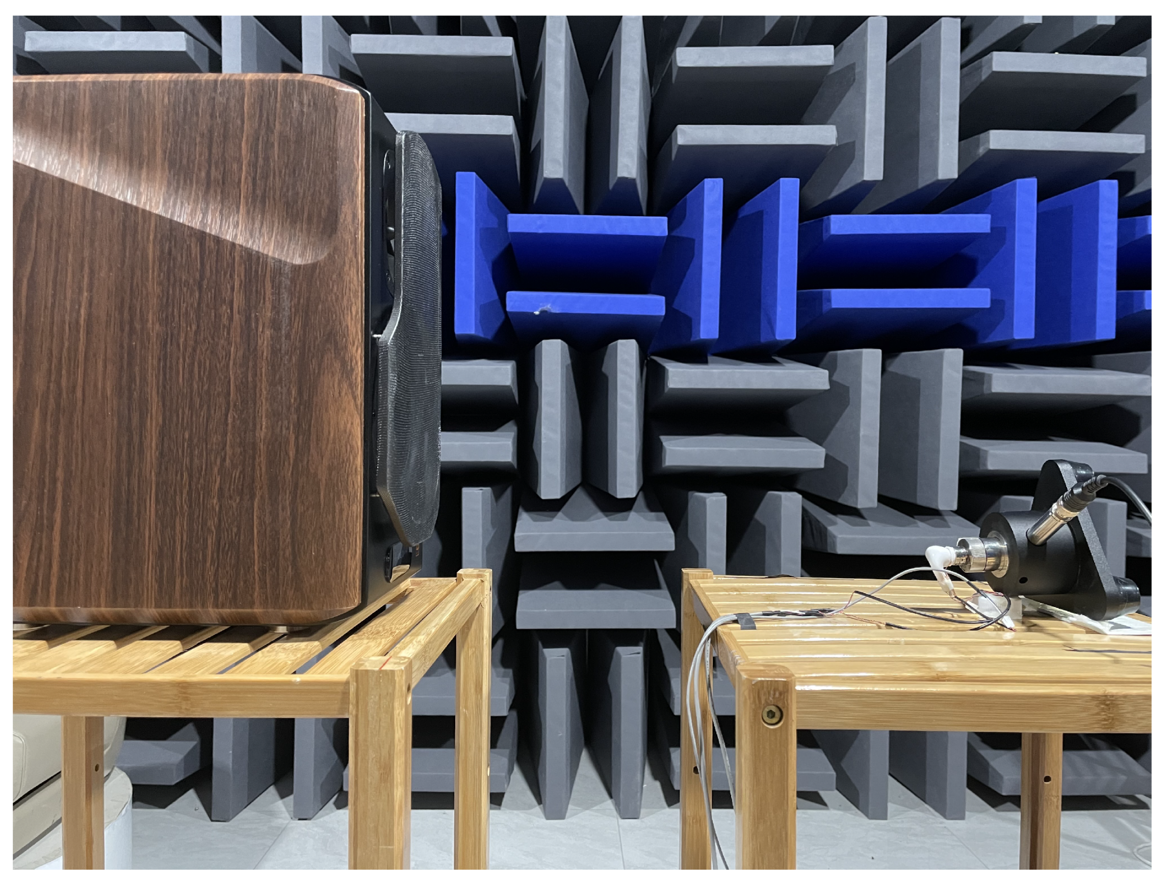
3.1. Experimental Setup Description

To investigate the fitting performance and its effect on the noise control performance of the proposed method, an earphone is used to collect the system response data. For this earphone, there is one microphone used as the reference sensor and one speaker used as the noise control speaker. The error microphone used in this experiment that measured the noise control performance is in an artificial ear shown in Figure 1. The artificial ear used is Hangzhou Aihua AWA6162 (IEC711).

The broadband noise control performance is considered in this section. Because of the limited dimension of the earphone, the delay in the signal path introduced by the electronic devices and anti-aliasing/reconstruction filters should be sufficiently small to achieve broadband noise control performance. Thus, the sampling rate of the data acquisition system and the noise control system was set to 48 kHz. Although the sampling rate is high (48 kHz), the desired noise control band is set from 50 Hz to 3 kHz for practical considerations. When measuring and computing the system responses, two million sampling points (about 42 s) are acquired and a hamming window of 48,000 points (around 1 s) is used for averaging with 50% overlap.

When the acoustic feedback path effect is canceled by an estimate of the acoustic feedback path, the block diagram of the ANC system installed in the tested earphone is shown in Figure 2. $\overrightarrow{x}$ denotes the noise signals from the primary noise source at the reference microphone location. White noise played by the speaker is used as the noise signal at the noise source in this experimental setup. $\overrightarrow{y}$ denotes the output of the noise control filter and $\mathbf{W}$. ${\mathbf{G}}_e$ denotes the secondary path which is the acoustical response of the secondary source at the error sensor position. The frequency responses of the measured secondary path are shown in Figure 3. ${\overrightarrow{d}}_e$ denotes the disturbance signals and $\overrightarrow{e}$ denotes the sum of primary and secondary sound fields at error sensor locations, whose total power is attenuated by the ANC system.

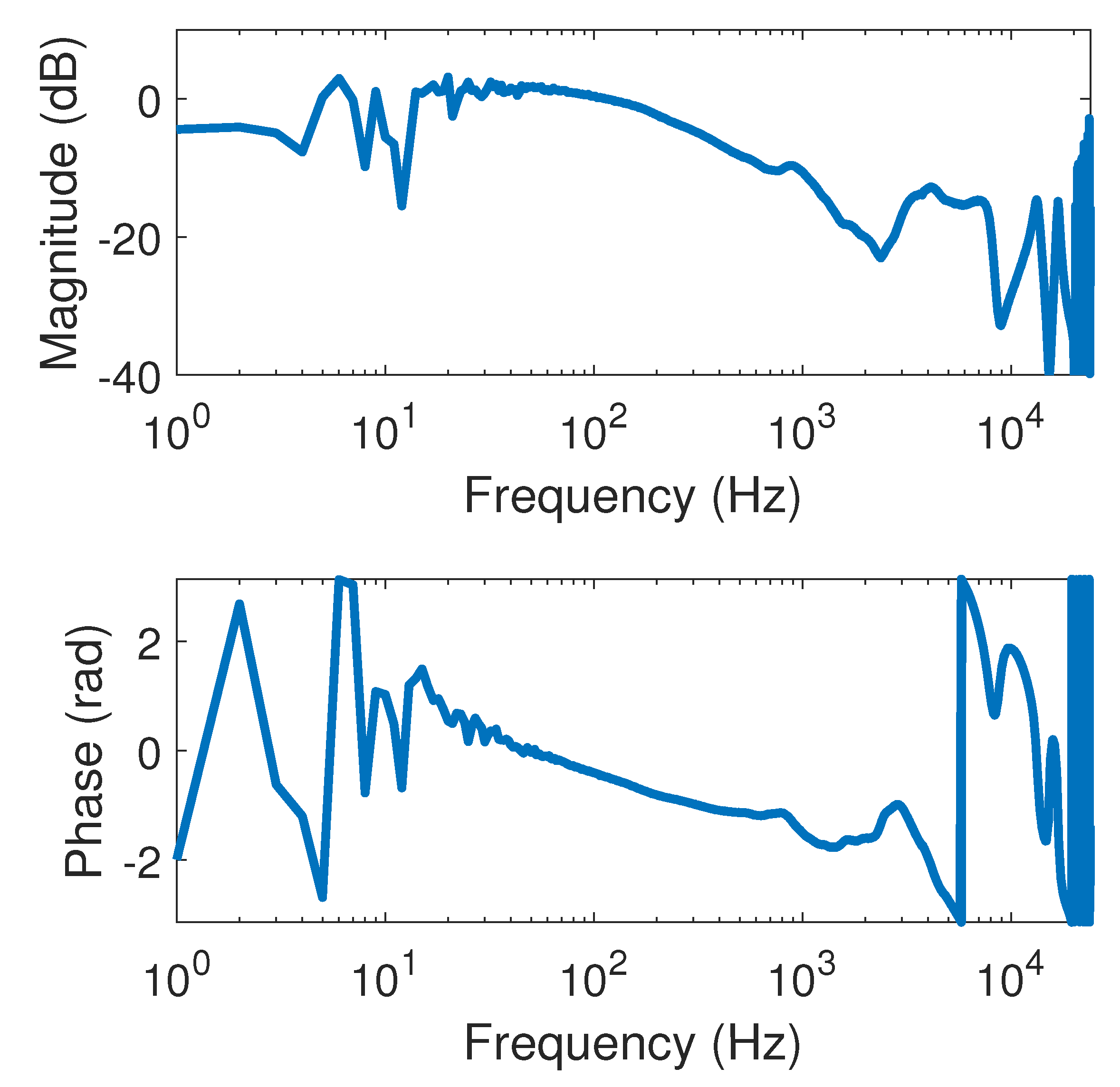
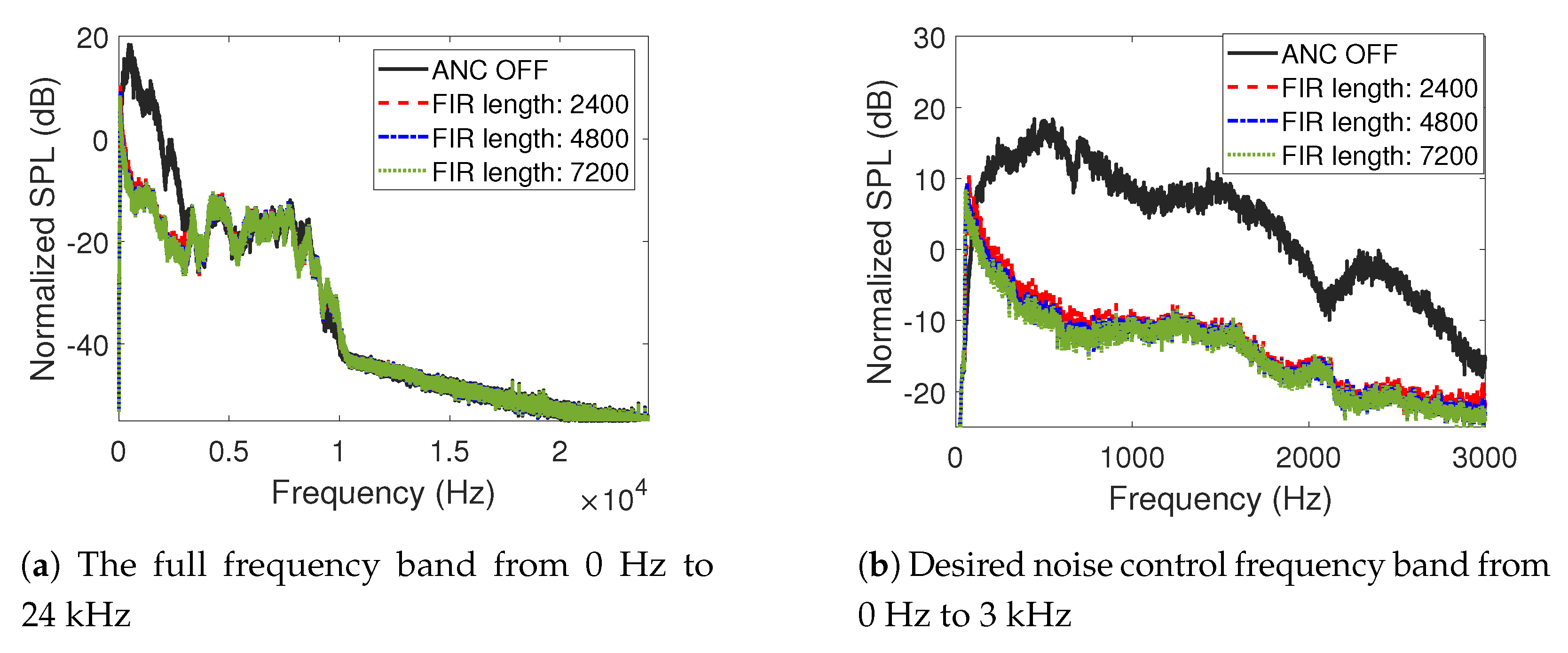
3.2. Comparison of Fitting Accuracy and Noise Control Performance

Because the desired noise control band is from 50 Hz to 3 kHz and the sampling rate is 48 kHz, which is much higher than the desired noise control band, some constraints, e.g., the filter responses amplitude constraints or the disturbance enhancement constraints should be applied at the higher frequency band to prevent the amplification of the high-frequency noises outside the desired noise control frequency band. Thus, the time-domain coefficients of the noise control filter $\mathbf{W}$ were designed firstly using an FIR filter structure with constrained optimal filter design methods [4,5]. Since the FIR filter is not the filter implemented in real-time, a sufficiently large order should be chosen. Thus, the FIR filter length is increased until the noise control performance cannot be improved any further. The nominal noise control performance using the designed FIR filter is shown in Figure 4 and Figure 5. From Figure 4, the designed FIR filter can achieve satisfactory noise control performance in the desired noise control frequency band and does not amplify noises outside the desired noise control frequency band. Figure 5 demonstrates that a large filter length (i.e., 7200) is needed because, compared with using 2400 and 4800 coefficients, using 7200 coefficients (equivalent to 0.15 s in the time-domain filter response length) can still improve the noise control performance, especially around the lower frequency band (3–4 dB better than 2400 coefficients case and around 1 dB better than 4800 coefficient cases). Since the improvement from using 4800 coefficients to using 7200 coefficients are not significant, 7200 coefficients are considered sufficient for this ANC application. The impulse response and frequency response of the designed FIR filter using 7200 coefficients are shown in Figure 6.

Although using 7200 coefficients can achieve satisfactory noise control performance at the desired frequency band without amplifying noises outside the frequency band, the real-time computational requirement is significant if a 7200-point FIR filter is implemented at a 48 kHz sampling rate. Thus, an IIR filter structure should be used to fit the responses of this 7200-point FIR filter. When using the IIR filter structure to fit the pre-designed FIR filter in Figure 6, the order of the numerator polynomial is set to be equal to the order of the denominator polynomial. Because the desired noise control (50 Hz to 3 kHz) is relatively narrow compared with the full band, 100 times higher weighting is applied to frequencies below 3 kHz to ensure an accurate fitting in the desired noise control band. When using the proposed method, a condition number higher than ${10}^{12}$ is considered large and the estimated gradient is used. Since the condition number is used as a threshold and the computation of coefficients does not need the exact value of the condition number, efficient estimates of condition numbers will be sufficient, e.g., the rcond() function in Matlab [21].

When using the traditional method, if the order of the IIR filter is chosen to be higher than 64, the algorithm cannot converge to a stable IIR filter. However, the proposed method can successfully fit the frequency responses using IIR filters with higher orders (e.g., 128 or 256). The comparison between pre-designed FIR filter frequency responses and the fitted IIR filter frequency responses using different methods and filter orders are shown in Figure 7a. From Figure 7a, all methods and filter orders can achieve satisfactory overall fitting accuracy for the whole frequency band, especially at higher frequencies. A zoomed-in frequency band from 100 Hz to 800 Hz is shown in Figure 7b to have a clearer comparison of the fitting accuracy. It demonstrates that during this relatively lower frequency range, the IIR filter fitted using the proposed method has a much better fitting accuracy compared with that of using the traditional method because the proposed method enables a higher-order stable IIR filter to be fitted. The comparison of nominal noise control performance using the traditional method and the proposed method is shown in Figure 8 for the full frequency band and the desired noise control band. The zoomed-in frequency band from 100 Hz to 800 Hz is also shown in Figure 9. This demonstrates that the proposed method can achieve a better noise control performance compared with the traditional method, especially for certain frequency bands, e.g., 3–5 dB better from 400 Hz to 600 Hz.

4. Discussion and Conclusions

In this article, a stable IIR fitting approach in high-order ANC applications is proposed by improving Brandenstein and Unbehauen’s method [19,20] such that the stability of the designed IIR filter can be guaranteed without implementing root-finding. A gradient-based searching method is proposed in this article in addition to the original solving approach in BU’s method such that convergence can be guaranteed, which is more applicable in practical applications. Practical approaches to obtain the required maximum phase weighting function and compute the optimal IIR filter numerator coefficients are also proposed in this article. An ANC system installed on an earphone prototype is used to investigate the performance of the proposed method. The result shows that the proposed improved IIR filter approximation method can achieve better fitting accuracy and noise control performance compared with the traditional IIR fitting approach.

Besides the fitting of the noise control filter, the proposed method can also be used for fitting secondary paths and acoustic feedback paths to further reduce real-time computations. Moreover, the proposed method can be used for fitting the secondary paths and acoustic feedback paths in both non-adaptive and adaptive applications.

Since no root relocation is required during the fitting process, the proposed method is more efficient and reliable and it may be extended in the real-time continuous redesign process where a noise control filter is designed by solving the optimal filter coefficients continuously [22].

References

- Bean, J.; Schiller, N.; Fuller, C. Numerical Modeling of an Active Headrest. In Proceedings of the INTER-NOISE and NOISE-CON Congress and Conference Proceedings, Hong Kong, China, 27–30 August 2017; Institute of Noise Control Engineering: Washington, DC, USA, 2017; Volume 255, pp. 4065–4075. [Google Scholar]
- Cheer, J.; Elliott, S.J. Multichannel control systems for the attenuation of interior road noise in vehicles. Mech. Syst. Signal Process. 2015, 60, 753–769. [Google Scholar] [CrossRef]
- Kajikawa, Y.; Gan, W.S.; Kuo, S.M. Recent advances on active noise control: Open issues and innovative applications. Apsipa Trans. Signal Inf. Process. 2012, 1, e3. [Google Scholar] [CrossRef]
- Zhuang, Y.; Liu, Y. Constrained optimal filter design for multi-channel active noise control via convex optimization. J. Acoust. Soc. Am. 2021, 150, 2888–2899. [Google Scholar] [CrossRef] [PubMed]
- Zhuang, Y.; Liu, Y. A numerically stable constrained optimal filter design method for multichannel active noise control using dual conic formulation. J. Acoust. Soc. Am. 2022, 152, 2169–2182. [Google Scholar] [CrossRef] [PubMed]
- Shi, D.; Gan, W.S.; He, J.; Lam, B. Practical implementation of multichannel filtered-x least mean square algorithm based on the multiple-parallel-branch with folding architecture for large-scale active noise control. IEEE Trans. Very Large Scale Integr. (Vlsi) Syst. 2019, 28, 940–953. [Google Scholar] [CrossRef]
- Ho, C.Y.; Shyu, K.K.; Chang, C.Y.; Kuo, S.M. Development of equation-error adaptive IIR-filter-based active noise control system. Appl. Acoust. 2020, 163, 107226. [Google Scholar] [CrossRef]
- Wu, L.; Qiu, X.; Guo, Y. A generalized leaky FxLMS algorithm for tuning the waterbed effect of feedback active noise control systems. Mech. Syst. Signal Process. 2018, 106, 13–23. [Google Scholar] [CrossRef]
- Lam, B.; Gan, W.S.; Shi, D.; Nishimura, M.; Elliott, S. Ten questions concerning active noise control in the built environment. Build. Environ. 2021, 200, 107928. [Google Scholar] [CrossRef]
- Bai, M.R.; Lin, Y.; Lai, J. Reduction in electronic delay in active noise control systems—A multirate signal processing approach. J. Acoust. Soc. Am. 2002, 111, 916–924. [Google Scholar] [CrossRef] [PubMed]
- Rout, N.K.; Das, D.P.; Panda, G. Computationally efficient algorithm for high sampling-frequency operation of active noise control. Mech. Syst. Signal Process. 2015, 56, 302–319. [Google Scholar] [CrossRef]
- Parks, T.W.; Burrus, C.S. Digital Filter Design; Wiley-Interscience: Hoboken, NJ, USA, 1987. [Google Scholar]
- Steiglitz, K.; McBride, L. A technique for the identification of linear systems. IEEE Trans. Autom. Control. 1965, 10, 461–464. [Google Scholar] [CrossRef]
- Ljung, L. System Identification-Theory for the User, 2nd ed.; Ptr Prentice-Hall: Upper Saddle River, NJ, USA, 1999. [Google Scholar]
- Levy, E. Complex-curve fitting. IRE Trans. Autom. Control. 1959, AC-4, 37–43. [Google Scholar] [CrossRef]
- Dennis, J.E., Jr. Rb Schnabel Numerical Methods for Unconstrained Optimization and Nonlinear Equations; Society for Industrial and Applied Mathematics: Philadelphia, PA, USA, 1983. [Google Scholar]
- Calvetti, D.; Reichel, L. On the evaluation of polynomial coefficients. Numer. Algorithms 2003, 33, 153–161. [Google Scholar] [CrossRef]
- Sitton, G.A.; Burrus, C.S.; Fox, J.W.; Treitel, S. Factoring very-high-degree polynomials. IEEE Signal Process. Mag. 2003, 20, 27–42. [Google Scholar] [CrossRef]
- Brandenstein, H.; Unbehauen, R. Least-squares approximation of FIR by IIR digital filters. IEEE Trans. Signal Process. 1998, 46, 21–30. [Google Scholar] [CrossRef]
- Brandenstein, H.; Unbehauen, R. Weighted least-squares approximation of FIR by IIR digital filters. IEEE Trans. Signal Process. 2001, 49, 558–568. [Google Scholar] [CrossRef]
- Anderson, E.; Bai, Z.; Bischof, C.; Blackford, L.S.; Demmel, J.; Dongarra, J.; Du Croz, J.; Greenbaum, A.; Hammarling, S.; McKenney, A.; et al. LAPACK Users’ Guide; Society for Industrial and Applied Mathematics: Philadelphia, PA, USA, 1999. [Google Scholar]
- Zhuang, Y.; Liu, Y. An adaptive constrained multi-channel active noise control filter design approach using convex cone optimization. In Proceedings of the INTER-NOISE and NOISE-CON Congress and Conference Proceedings, Grand Rapids, MI, USA, 12–14 June 2017; Institute of Noise Control Engineering: Washington, DC, USA, 2023. [Google Scholar] [CrossRef]
Disclaimer/Publisher’s Note: The statements, opinions and data contained in all publications are solely those of the individual author(s) and contributor(s) and not of MDPI and/or the editor(s). MDPI and/or the editor(s) disclaim responsibility for any injury to people or property resulting from any ideas, methods, instructions or products referred to in the content. |
© 2023 by the authors. Licensee MDPI, Basel, Switzerland. This article is an open access article distributed under the terms and conditions of the Creative Commons Attribution (CC BY) license (https://creativecommons.org/licenses/by/4.0/).
Share and Cite
Zhuang, Y.; Liu, Y. A Stable IIR Filter Design Approach for High-Order Active Noise Control Applications. Acoustics 2023, 5, 746-758. https://doi.org/10.3390/acoustics5030044
Zhuang Y, Liu Y. A Stable IIR Filter Design Approach for High-Order Active Noise Control Applications. Acoustics. 2023; 5(3):746-758. https://doi.org/10.3390/acoustics5030044
Chicago/Turabian StyleZhuang, Yongjie, and Yangfan Liu. 2023. "A Stable IIR Filter Design Approach for High-Order Active Noise Control Applications" Acoustics 5, no. 3: 746-758. https://doi.org/10.3390/acoustics5030044
APA StyleZhuang, Y., & Liu, Y. (2023). A Stable IIR Filter Design Approach for High-Order Active Noise Control Applications. Acoustics, 5(3), 746-758. https://doi.org/10.3390/acoustics5030044