Active Control of the Reflection Coefficient of an Underwater Surface

Abstract

From a strategic point of view, it is essential to protect underwater vehicles from being detected by opponents. Modern mono- or bistatic sonar systems are capable of precisely determining the position of a watercraft. In order to triangulate the positions of watercrafts, the sonar sends out acoustic signals that are reflected by the vehicles’ surfaces. These deflected sound waves are subsequently detected and evaluated. How well an object can be detected using a sonar can be measured according to the target strength. Through their shape, construction and choice of materials, modern underwater vehicles are optimized in relation to minimizing their radiated and reflected sound waves; in this way, their target strength is minimized. These passive measures are particularly effective in the medium- and high-frequency range down to 1500 Hz. To effectively reduce reflections at lower frequencies, an active system is developed in this study and evaluated in a laboratory test with a water-filled impedance tube. The incident sound waves were measured in front of an active surface and then processed using an adaptive control system based on an FPGA platform. The system operates with a very thin piezoceramic applied to the surface in order to minimize the reflections of the sound waves. The laboratory tests showed the high effectiveness of the system under the influence of sonar-like signals.

1. Introduction

The main tactical advantage of a submarine is its possibility to operate undetected by an enemy. To conceal the sound signature of a submarine, researchers and manufactures reduce the emitted sound power of modern vehicles. In addition to passive measures, such as adding damping materials, active noise control (ANC) has already been proposed for submarines with diesel engines. This method shows a promising noise reduction of the engine exhaust system [1]. But even if the vehicle itself operates quietly, it can still be detected using an active sonar. Developed in the First World War for submarine detection, this sonar has evolved into the modern mono- and bistatic systems through continuous improvements [2]. The risk of detection using an active sonar is directly dependent on the object’s target strength. The target strength, often considered as an object’s acoustic size, is not only dependent on the dimensions, but also on the material, geometric and inner structure of the object [3,4]. The majority of studies researching the target strength of submarines are based on numerical methods to test designs, since measurements are often not feasible due to high costs and confidentiality constraints. In [5,6], the benchmark target echo strength simulation (BeTSSi) is used. Nolte et al.’s study focuses on a comparison of the performance of different solvers and numerical methods. Sathish et al. used the Helmholtz–Kirchhoff method and FEM in their studies, in which they concluded that an anti-reflection coating should be used to absorb high-frequency sonar signals. In [7], the authors Fang et al. drew the same conclusion based on a different submarine model and simulation environment. Kwonn et al., in [8], also validated their simulations based on the Kirchhoff approximation, using measurements of a downscaled model. They claim to be able to predict the effect of material and geometric changes on the target strength with their simulation. These numerical studies all draw the same conclusions and suggest the use of absorbing materials as coatings to dampen higher-frequency sonar signals, thus decreasing the target strength of submarines. Nonetheless, a major drawback of absorbing materials is that they require increasing the layer thickness as the sonar frequency is reduced. For lower frequencies, it is not feasible to rely on the absorption characteristics of the outer skin of a vehicle. Another strategy to reduce the target strength is to inhibit the reception of reflected signals by choosing a stealth form. This approach is well established and well known for military aircraft with stealth shapes that are optimized to avoid detection by radar. The goal of the stealth shape is to deflect the incident sound waves away from the radar’s or sonar’s direction. In the field of submarines, this concept is still under research and development. One example can be found in [9,10], where the authors carried out extensive simulations to compare the target strength of a stealth submarine form to a classic cylindrical shape. The investigation based on BeTSSi also includes absorbing materials on the outer hull and distinct oceanic regions around the world. However, at frequencies below 1500 Hz, the desired effect is less pronounced, and parts of the sound waves are directly reflected to the sonar’s position. To effectively protect against detection—even in the frequency range below 1500 Hz—active measures could be a promising solution. A classic ANC system minimizes the sound pressure locally by applying the principle of the destructive interference of sound waves. In the present report, the wall impedance of the surface shall be manipulated in order to minimize reflections of the incident sound waves. This method is often called active impedance control (AIC) and was demonstrated for an air-filled impedance tube in [11,12,13]. 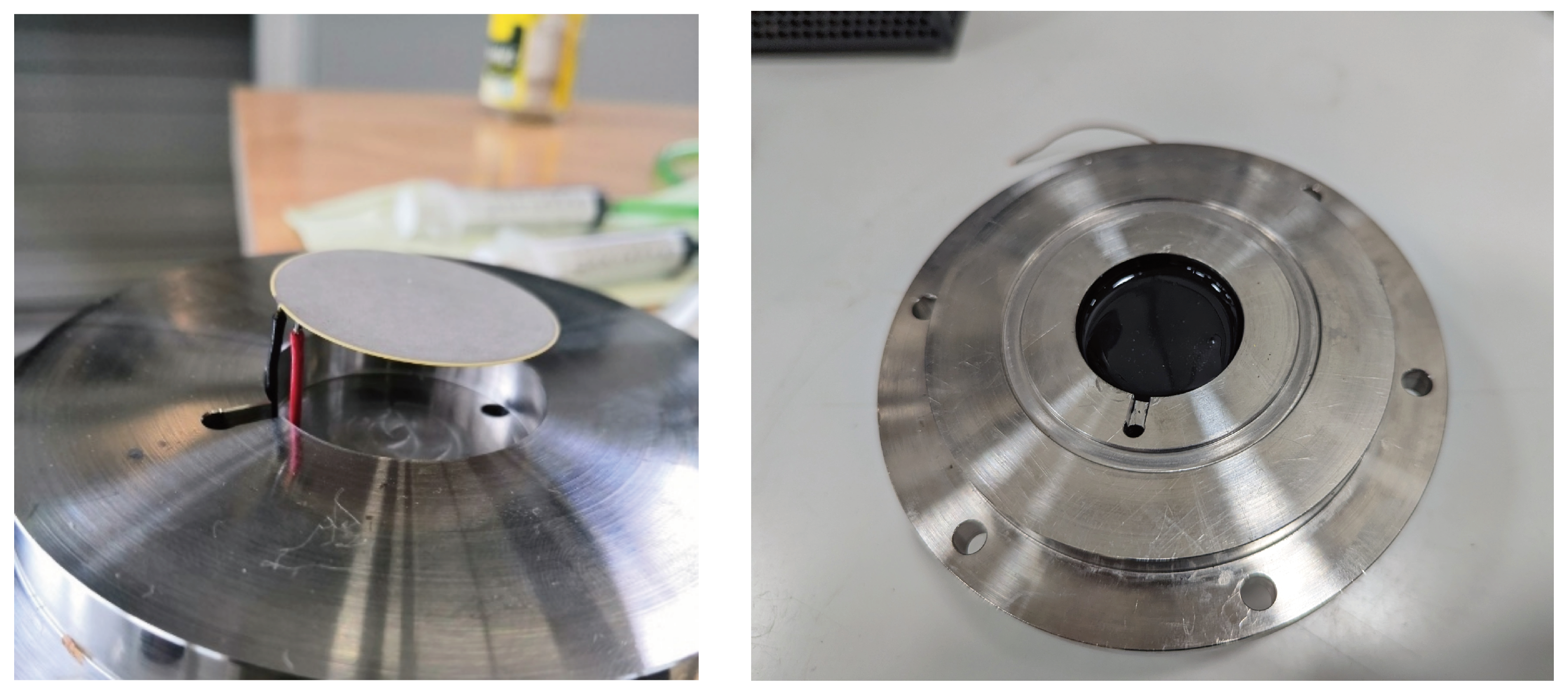As part of this project, a preliminary study [14] was conducted to develop a demonstrator to minimize the reflective properties of a submerged steel surface. This was based on a water-filled impedance tube that contained a Tonpilz transducer at one end as the primary actuator in order to emulate the sonar signal. The opposite end was realized using a thin piezoceramic as a secondary actuator representing the vehicle surface. Several sensors were located in the tube to measure the sound pressure distribution. The piezo-actuator was controlled by means of an adaptive controller in the frequency domain, the effectiveness of which was demonstrated in a series of experiments. The presented system in [14] had several drawbacks, such as its dependence on the internal reference of the signal generator and the limitation to only stationary tonal signals.

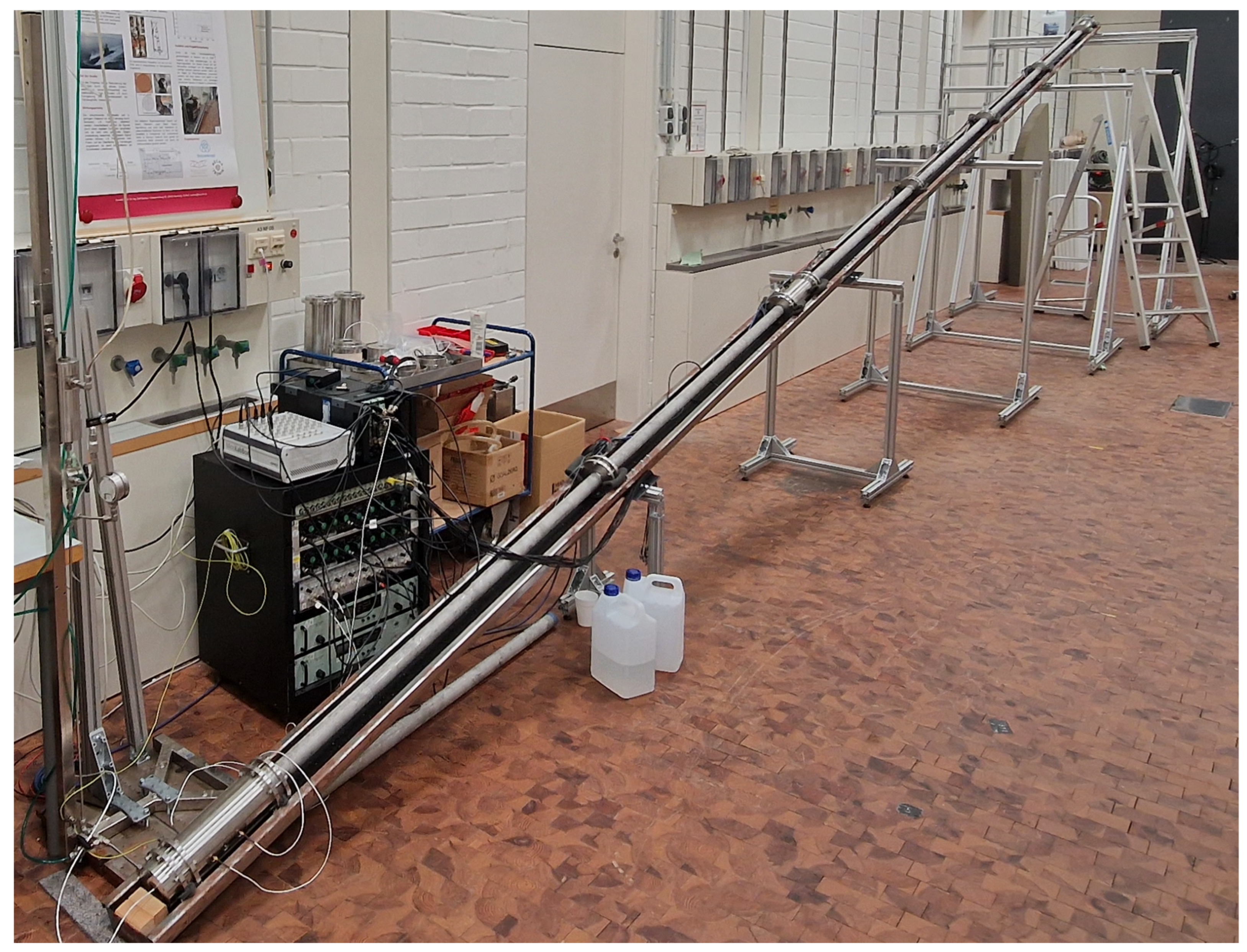
In this paper, the adaptive control system is redesigned and implemented in the time domain to improve its capabilities. The measurement setup is extended to an impedance tube up to 9.81 m, which can be equipped with several sensor modules. This allows for the detection of the incident sound wave with physical sensors, which is necessary for adapting the active control system to vehicles in the future. As a result, the system is able to minimize the reflections of sonar-like signals inside the impedance tube and delivers a proof-of-concept for further research on active surfaces for submarines.

2. Materials and Methods

2.1. Implementation

As mentioned previously, using an actuator to reduce acoustic wave reflections is called AIC, which is described in [11,12,13]. This method requires the decomposition of the sound field into an incident and reflected wave and can be implemented in the frequency or time domain. The high speed of sound in water results in low latency requirements that can be challenging when the signals have to be first transformed into the frequency domain. For this reason, AIC should be implemented in the time domain. Figure 1 shows a schematic drawing of the measurement setup, which is used to explain the operation of the AIC system.

An estimation of the incident and reflected waves can be achieved by measuring the pressure at two hydrophones, which are arranged at a distance of $\Delta s$ from each other. Hydrophone 1.1 has a distance from the wall of $s_1$, and hydrophone 1.2 has a distance from the wall of $s_2$. According to [12], the signals $h_{1.1}$ and $h_{1.2}$ are measured at the hydrophones in the time domain and can be expressed in terms of

$$h_{1.1}\left(t\right)=A_1[p_i(t+\frac{s_1}{c})+p_r(t-\frac{s_1}{c})]$$

(1)

and

$$h_{1.2}\left(t\right)=A_2[p_i(t+\frac{s_1+\Delta s}{c})+p_r(t-\frac{s_1+\Delta s}{c})],$$

(2)

where $A_1$ and $A_2$ are weighting factors describing the respective sensitivities of the hydrophones. Using the speed of sound c, the acoustic delay $\tau$ between the two hydrophone positions $s_1$ and $s_2$ can be calculated with

$$\tau =\frac{\Delta s}{c}.$$

(3)

The time signals $h_{1.1}^{\prime }\left(t\right)$ and $h_{1.2}^{\prime }\left(t\right)$ delayed by $\tau$ can thus be formulated in terms of the incident and reflected sound waves as follows:

$$h_{1.1}^{\prime }\left(t\right)=A_1[p_i(t+\frac{s_1-\Delta s}{c})+p_r(t-\frac{s_1+\Delta s}{c})]$$

(4)

and

$$h_{1.2}^{\prime }\left(t\right)=A_2[p_i(t+\frac{s_1}{c})+p_r(t-\frac{s_1+2\Delta s}{c})].$$

(5)

Assuming the sensitivities $A_1$ and $A_2$ of the two hydrophones are identical, the difference between Equations (2) and (4), denoted here as $u\left(t\right)$, and the difference between (1) and (5), denoted here $v\left(t\right)$, are calculated as follows:

$$u\left(t\right)=A[p_i(t+\frac{s_1+\Delta s}{c})-p_i(t-\frac{s_1-\Delta s}{c})]$$

(6)

and

$$v\left(t\right)=A[p_r(t-\frac{s_1}{c})-p_r(t-\frac{s_1+2\Delta s}{c})],$$

(7)

respectively. It is obvious that $u\left(t\right)$ consists only of components of the incident sound wave and $v\left(t\right)$ is correspondingly composed exclusively of components of the reflected sound wave. Thus, $u\left(t\right)$ and $v\left(t\right)$ provide an estimate of the incident and reflected sound waves according to

$$p_i\left(t\right)\approx u\left(t\right)=h_{1.2}\left(t\right)-h_{1.1}^{\prime }\left(t\right)$$

(8)

and

$$p_r\left(t\right)\approx v\left(t\right)=h_{1.1}\left(t\right)-h_{1.2}^{\prime }\left(t\right).$$

(9)

To calculate the complex reflection coefficient $\underline{r}$, $u\left(t\right)$ and $v\left(t\right)$ would then have to be transformed into the frequency domain [12]. However, this study shows that estimating the incident and reflected sound waves using the time signals $u\left(t\right)$ and $v\left(t\right)$ is sufficient for an adaptive controller to reduce the reflections of the active surface. The calculation of the Equations (8) and (9) can be performed with analog elements, or the hydrophone signals are directly sampled and all calculations are performed in the digital domain, resulting in the time discrete signals $u\left(n\right)$ and $v\left(n\right)$. In this study, distilled water at room temperature under normal atmospheric pressure was used. Its speed of sound was estimated as $c=1472\frac{\mathrm{m}}{\mathrm{s}}$. With a distance of 75 mm between sensors H1.1 and H1.3, which were primarily used in the measurements, the acoustic delay $\tau$ was equal to 50.95 μs. A digital control system with wave separation calculation needs to be at least able to represent $\tau$, resulting in a minimum sampling rate of $f_s$ = 19,627 Hz. Although it was not a focus of this study, it is worth noting that our measurement setup is capable of both pressurization and temperature control. Variations in these environmental variables predominantly affect the speed of sound, a critical factor that must be accounted for in an active system.

To actively control the wall impedance and thereby lower the reflection coefficient, the estimated reflected wave was fed to a normalized feedforward filtered-x least mean square (FxLMS) algorithm as an error signal. The update of the adaptive coefficient vector $\mathit{w}\left(n\right)$ for the next iteration step

$$\mathit{w}(n+1)=\mathit{w}\left(n\right)-\mu e\left(n\right){\mathit{x}}^{\prime }\left(n\right)$$

(10)

was performed, where $\mu$ represents the step size, $e\left(n\right)$ is the error signal and ${\mathit{x}}^{\prime }\left(n\right)$ is the buffered reference signal that was filtered by the estimation of the secondary path, hence the name filtered-x. Presumably, several signals are suitable as references for the feedforward controller in this study. In the laboratory experiment, the signal generated by the signal generator for the Tonpilz transducer could be used directly as an internal reference. This will likely result in the best performance of the active surface, but cannot be applied to a real world application where the signal generated by a sonar is unknown. However, it is possible to place another sensor module at a greater distance in front of the surface, at which point either the pressure or, according to Equations (1)–(8), the incident sound wave are measured. The FxLMS was extended via the power normalization of the step size to improve the convergence speed and stability. The resulting adaptive step size

$$\mu (n)=\frac{\alpha }{L\max \left[{\widehat{P}}_x^{\prime }\right(n),P_{\min }]},0<\alpha <2.$$

(11)

is calculated depending on the normalized step size parameter $\alpha$, the number of adaptive filter coefficients L and the power of the filtered reference signal. To compensate for large step sizes in the case of a small signal power of $x’\left(n\right)$, a minimum power $P_{min}$ was introduced to enhance stability. To avoid larger fluctuations in the estimated signal power,

$${\widehat{P}}_x^{\prime }\left(n\right)=(1-\beta ){\widehat{P}}_x(n-1)+\beta {\mathbf{x}}^2\left(n\right).$$

(12)

was averaged using the smoothing parameter $\beta$. Therefore, the smoothing parameter $\beta$ could be used to tune the considered time window for the average power calculation. If $\beta$ is small, a long time window is chosen, and smoother power estimates occur, which can be beneficial for stationary signals. If the reference signal is non-stationary, a larger $\beta$ should be chosen to track rapid power changes. As a last measure, a leakage factor

$$\nu \left(n\right)=1-\mu \left(n\right)\gamma ,0<\gamma <1$$

(13)

complements the algorithm to improve stability, especially for tonal signals, by preventing the uncontrolled growth of the adaptive filter coefficients [15]. The advanced update term changes Equation (10) to

$$\mathit{w}(n+1)=\nu \left(n\right)\mathit{w}\left(n\right)-\mu \left(n\right)e\left(n\right){\mathit{x}}^{\prime }\left(n\right).$$

(14)

A detailed explanation of the implementation of the normalized FxLMS with leakage factor for FPGA platforms was described in [16,17] for various feedback systems and was validated for different ANC applications. This implementation is consistent with the described standard in [15]. The application in this current study required that the algorithm be changed to a feedforward configuration. In addition, the error signal and, if necessary, the reference signals are calculated on the FPGA according to the wave separation (Equations (8) and (9)). Due to the resonance effects of the measurement setup, it cannot be expected that the system will operate stably in every situation. For this reason, a reset of the algorithm was implemented in the design and was triggered if the system became unstable and the output reached a pre-specified threshold.

2.2. Measurement Setup

The measurement setup consists of a steel tube with an inner diameter of 35 mm, which has a variable length up to 9.81 m. The cut-on frequency, where the first corresponding cross mode appears, was around 21 kHz. This depends on the inner tube diameter and the speed of sound. Below this cut-on frequency, only plane sound waves were expected. The tube was divided into several modular segments. An incline angle of about 14° was chosen for the complete setup to ensure self-venting. This was mandatory, as bubbles or air pockets can strongly influence the measurements. At one end of the tube, a Tonpilz transducer was installed, which simulated the active sonar. The opposite end of the tube was realized using a 0.2 mm thick piezoceramic in front of a steel wall, which represented the surface of the underwater vehicle. The piezoceramic, shown in Figure 2 (Left), was embedded in an acoustic potting compound, AptFlex F21, to protect it from mechanical and chemical damage. The potting compound also ensured the electrical isolation of the contacted piezoceramic disc from the steel housing. On the right hand side, the finished actuator is shown.

The piezoceramic works in the lengthwise direction and was fully electrically contacted on the top and bottom. The cables were then guided through the back of the steel housing. This active termination module was directly attached to the first measurement module, which is shown in Figure 3.

These modules can be equipped with up to three pressure sensors and were manufactured for these measurements. A photo of the full-length measurement setup in the laboratory is displayed in Figure 4.

There was a total number of six hydrophones, pressure sensors PCB Piezotronics S112A22, installed into the two modules at different positions in the tube. Within one module, the hydrophones were not equidistantly arranged in order to avoid special cases where the nodes of the wave field were at all sensor positions at the same time. The exact positions of the sensors, relative to the end of the tube containing the piezoceramic (see Figure 1), are listed in

Table 1. Positions of the pressure sensors inside the tube.

	H1.1	H1.2	H1.3	H2.1	H2.2	H2.3
Distance to piezoceramic surface in m	0.076	0.107	0.151	1.841	1.874	1.916

.

The whole tube lay on a rubber insert in a folded steel construction as shown. At the flanges, the sides were insulated with additional foam sheets. An analog filter bank from the I.E.D company was used for signal conditioning as an aliasing and reconstruction filter. The low-pass filters were second-order Bessel filters set to a cut-off frequency of 8 kHz. Additional high-pass filters, Kemo VBF/8 set to 200 Hz, were applied to the reference signals. This was necessary to reduce the effects of the mains frequency of 50 Hz and multiples of it on the reference signals in the measurement. The Tonpilz transducer and the experimental piezo-actuator were each driven by a Brüel & Kjær 2732 amplifier. The wave separation and the adaptive algorithm were executed on a dSpace Microlabbox. This rapid prototyping platform was equipped with a Xilinx Kintex-7 XC7K325T FPGA and had 16-bit analog-to-digital converters (ADC) and digital-to-analog converters (DAC) with a sampling rate of up to 1 MHz. For data analysis and primary signal generation, Brüel & Kjær frontend modules were used. The reflection coefficient was calculated using a custom script in the Brüel&Kjær Pulse Labshop software using the auto- and cross-correlation of the measured pressure signals.

3. Results

To get an overview of the sound field inside the tube and of the system properties, the Tonpilz transducer and the experimental piezo-actuator were first examined individually without active control. Both actuators were driven separately after each other using a sine sweep from 300 Hz to 1500 Hz with a frequency increase of $1.5\frac{\mathrm{Hz}}{\mathrm{s}}$. The amplifiers were set to an output voltage of 5 V in both cases. 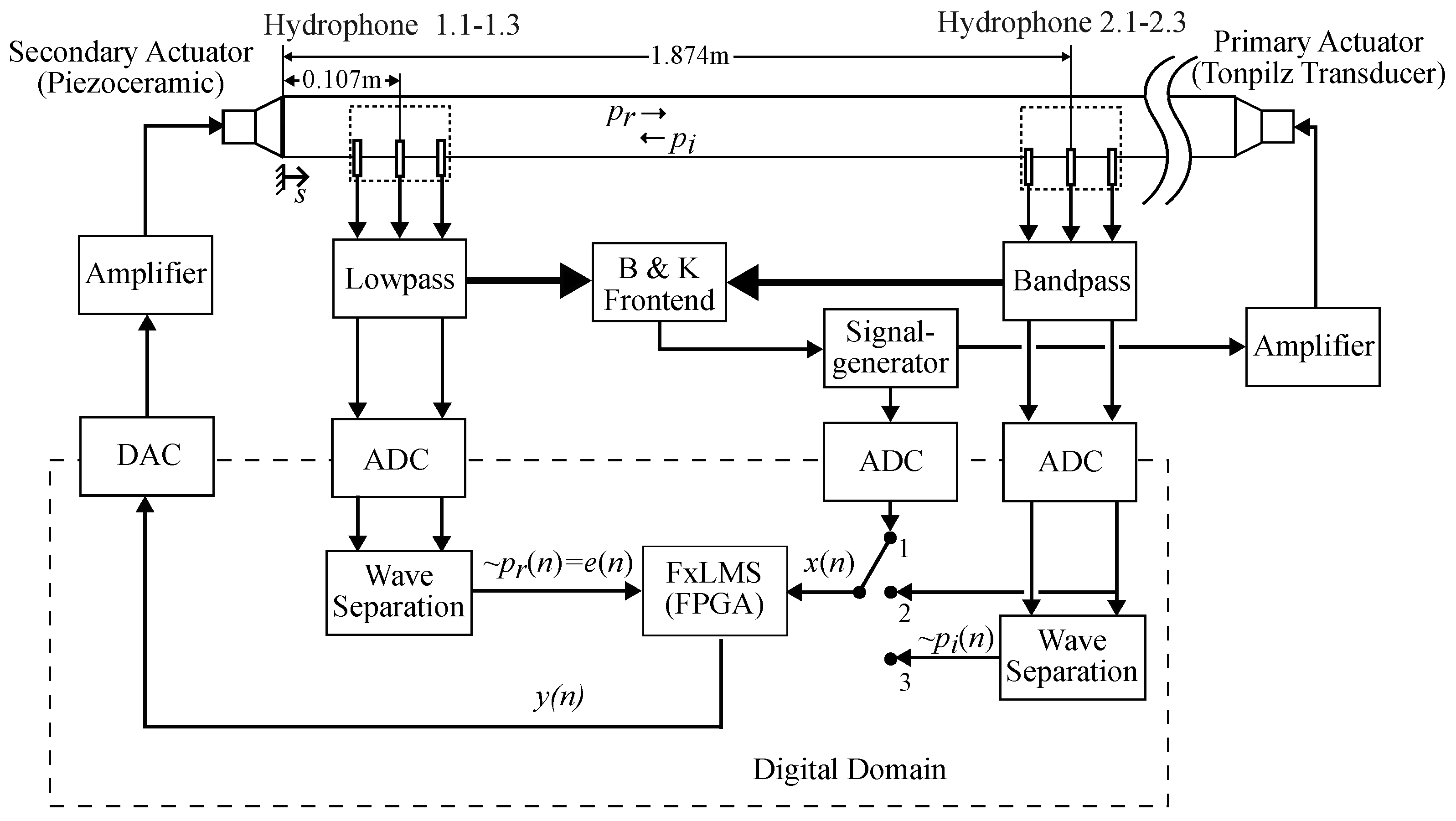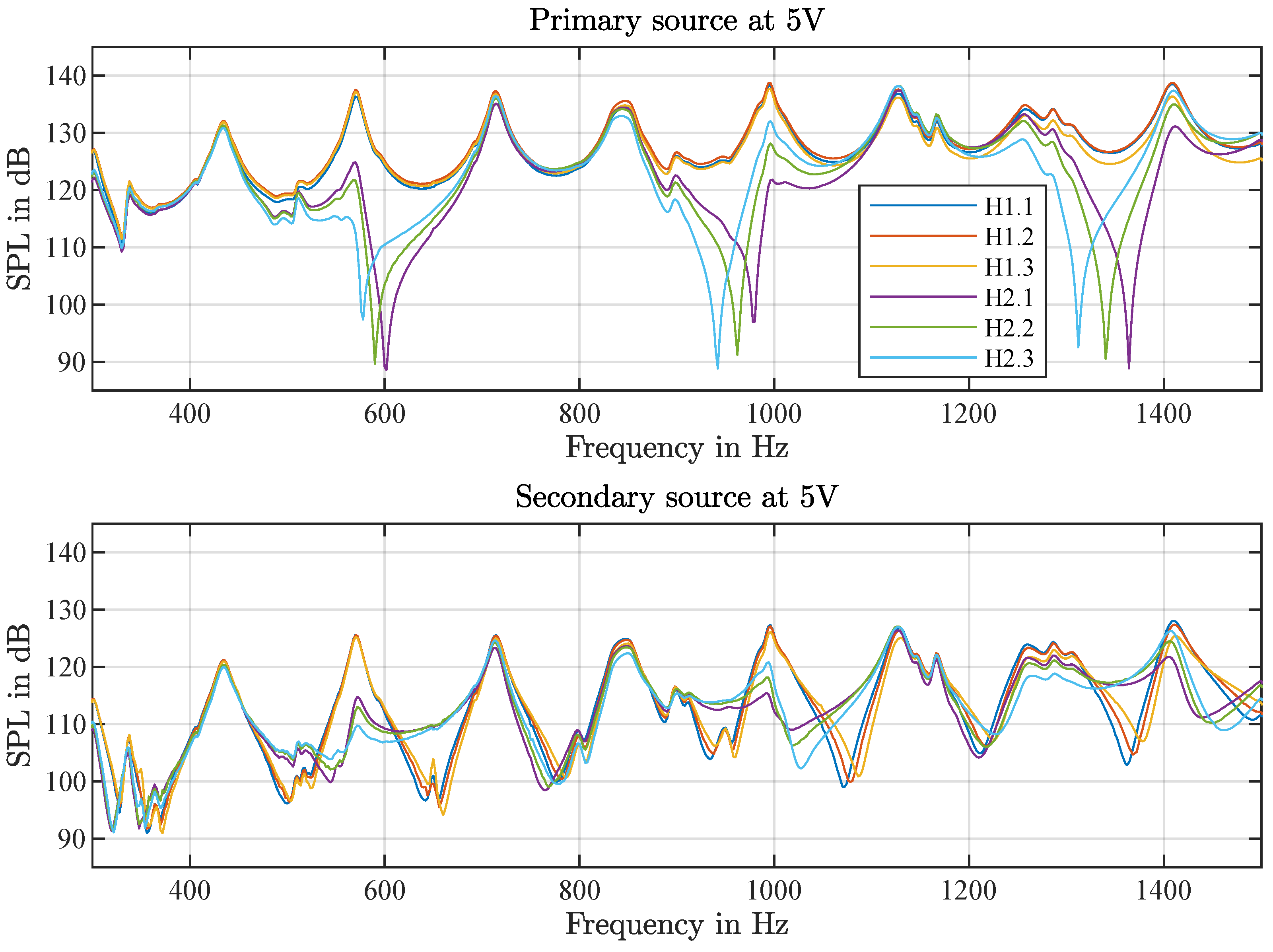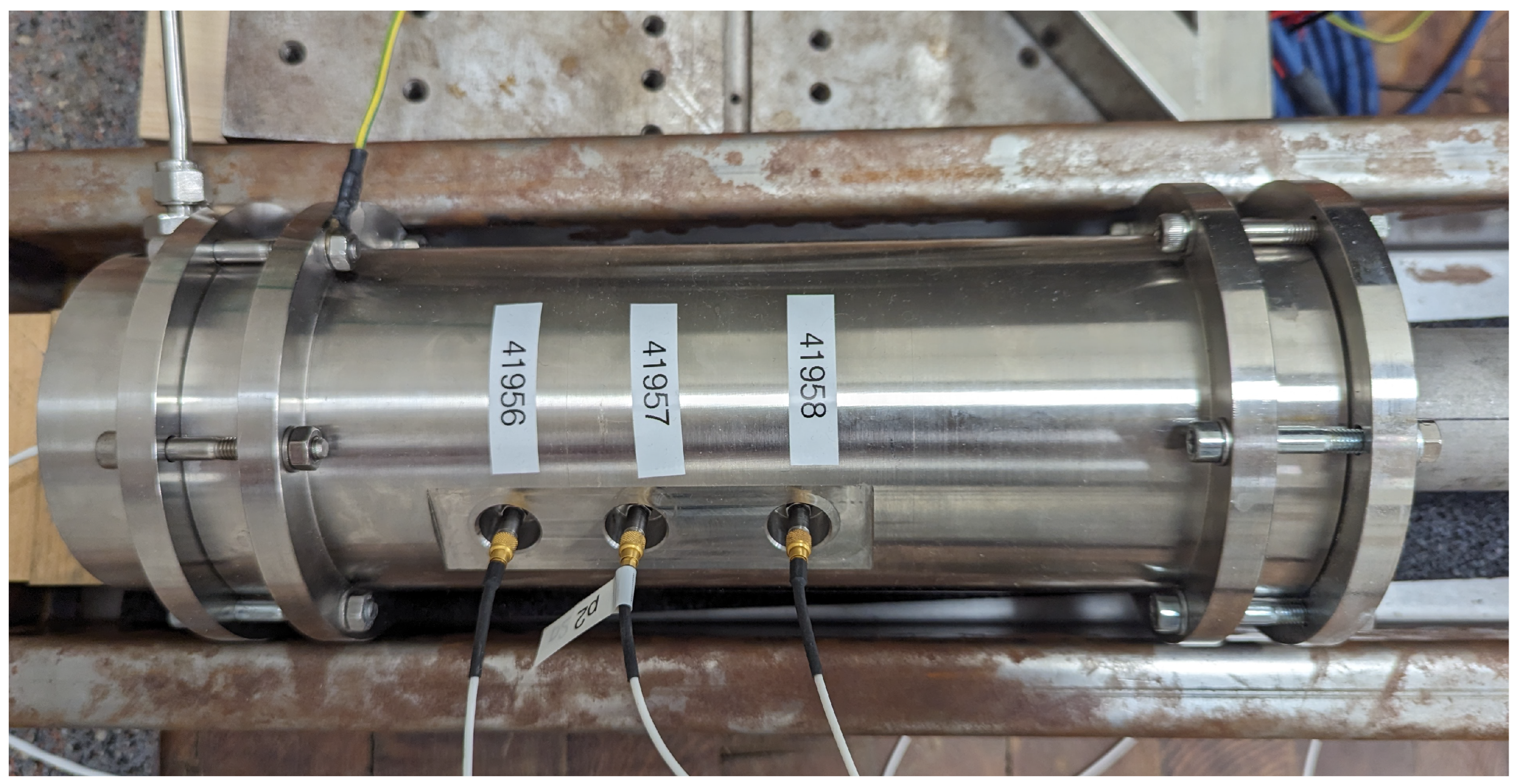Figure 5 shows a comparison of the measured sound pressure level (SPL) of all sensors generated by both actuators, respectively, located on opposite sides of the tube, as shown in Figure 1. The tube was configured to a length of 5.03 m, and the hydrophone positions are stated in Table 1. The primary reason for using a reduced length were resonance effects that will be further analyzed and discussed in the following.

When only the primary actuator (Tonpilz transducer) was active, there were significant minima of the SPL at the position of measurement module two. These minima occurred at the vibration nodes caused by standing waves inside the tube. Their positions within the tube depended on the wavelength and thus on the frequency. The arrangement of the piezoceramic on the steel construction realized a hard acoustic boundary condition and reflected the sound waves with minimal energy loss. This behavior can also be observed in the following investigation of the reflection coefficient. Comparing the sound pressure caused by the secondary actuator and by the Tonpilz transducer, different behaviors of the actuators can be observed. The 0.2 mm piezoceramic was less efficient than the Tonpilz using the same 5 V driving voltage, which is not surprising, because a Tonpilz transducer is optimized for sound radiation and typically actuated via a piezo stack (pp. 98–106, [18]). As a passive end element of the tube, the Tonpilz also resulted in a different boundary condition, absorbing more energy of the incident sound wave. As a result, the pressure minima occurring at measurement module two were less pronounced. The k resonance frequencies of a water column with sound pressure and sound velocity boundary conditions are as follows:

$$\begin{array}{c}\hfill f_k=k{\displaystyle \frac{c}{2l}}=k{\displaystyle \frac{1472\mathrm{m}/\mathrm{s}}{10.06\mathrm{m}}}\approx k146.3\mathrm{Hz}.\end{array}$$

(15)

This depended on the speed of sound c and the inner length of the tube l. The higher eigenfrequencies were at 293 Hz, 439 Hz, 586 Hz, 732 Hz, 879 Hz, 1024 Hz, 1172 Hz, 1317 Hz and 1465 Hz. These caused anomalies in the measured pressure with both actuators, which had a direct impact on the active system. These frequencies can be identified in Figure 5 as maxima of the SPL, independent of the actuator used. It should be noted that the pressure maximum around 1317 Hz was less defined compared to the other eigenfrequencies. Regardless of the actuator type selected, mode splitting was noticeable, as shown in Figure 5, for example, around 1172 Hz. This behavior could potentially be attributed to several factors. One possible explanation is the presence of residual air bubbles within the tube. Another consideration is the interaction occurring at the boundary between the water and the steel surface of the tube. Additionally, the interaction between the fluid acoustics within the tube, and the propagation of acoustic waves through the steel material of the tube, could also contribute to this phenomenon. In the next step, the results of the active system will be discussed. To achieve optimal results, the sampling rate $f_s$ was set to 40 kHz in the following experiments. A complete overview of the parameters of the experiment is presented in

Table 2. Parameters of the implementation.

${\mathit{f}}_{\mathit{s}}$	${\mathit{f}}_{\mathit{c}}$	Static Coefficients	Adaptive Coefficients	$\mathit{\alpha }$	$\mathit{\beta }$	$\mathit{\gamma }$	${\mathit{P}}_{\mathit{min}}$
40 kHz	8 kHz	128	128	0.0001	0.1	0.01	0.0001

.

In our study, the FxLMS parameters were not individually adjusted for each design iteration that used a different reference signal. This decision was made to facilitate a more straightforward and objective comparison of the results across various designs. Prior to the final experiments, we selected a set of parameters for the FxLMS algorithm based on empirical data and our prior experience.

The synthesis of the feedforward FxLMS including the wave separation resulted in a hardware utilization of the Xilinx Kintex-7 XC7K325T FPGA, as displayed in

Table 3. Resource utilization of the Xilinx Kintex-7 XC7K325T.

Type	Used	Available	Utilization
Configurable Logic Block Slices	8171	50,950	16.04%
Configurable Logic Block Slice LUTs	26,626	203,800	13.06%
Configurable Logic Block Slice Flip-Flops	25,330	407,600	6.21%
Block RAM Blocks 32 Kb	1	445	0.22%
Block RAM Blocks 16 Kb	4	890	0.45%
DSP Slices	61	840	7.26%

.

The resources with the highest usage were the configurable logic blocks (CLBs) and lookup tables (LUTs) with up to 16.04% of their available capacity being used. The resource utilizations of the other components were below 10%, leaving headroom for future experiments with more complex setups with multiple actuators and more sensors. All the following results are based on this configuration.

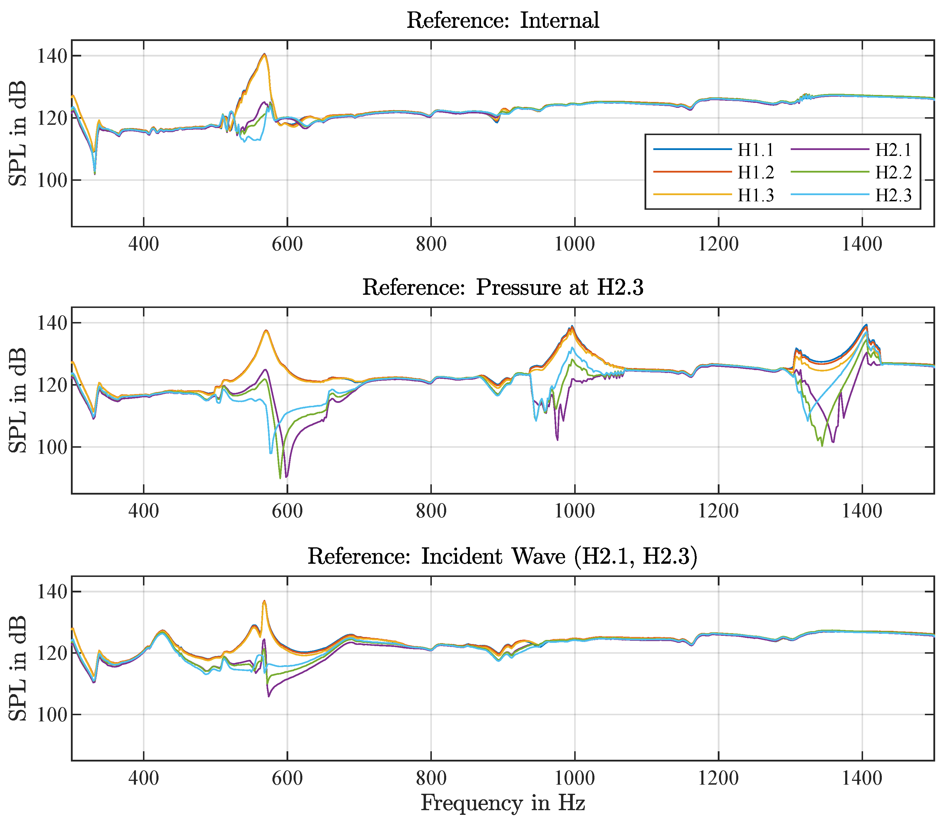
In the following measurements, the Tonpilz was again driven by the same 5 V sine sweep as in Figure 5 (Top). In addition, the adaptive control system was then active. The results of the measurements with the three types of reference signals are displayed in Figure 6.

The top row shows the system with the internal reference, the middle row is based on the measured SPL of H2.3 and the bottom uses a reference based on the incident sound wave calculated using Equation (8), using H2.1 and H2.3. The SPL with active control became mostly constant compared to Figure 5. The SPL rose slightly from around 115 dB below 400 Hz to 125 dB above 1400 Hz, showing a more efficient sound radiation of the transducers for higher frequencies. The equality of the sound pressure distribution indicated that the incident wave was no longer reflected at the piezoceramic. Therefore, no standing wave field was building up. The best results were achieved by the controller using the internal reference (Top), which was to be expected. Even in this case, the system showed some irregularities that corresponded to the resonance frequencies at 586 Hz, 879 Hz, 1172 Hz and 1317 Hz. The effects could also be observed with designs based on the other reference signals. The worst result at all sensors, in terms of a flat amplitude frequency response, was achieved by the controller using only a single pressure sensor as reference (Figure 6, Middle). Moreover, there were three frequency ranges of diverging amplitude frequency response, around 600 Hz, 950 Hz and 1350 Hz. These corresponded to the nodes at module 2, as seen in Figure 5 (Top). In this case, the SPL at the reference sensor was low and not representative of the incident sound wave arriving at the active surface. As a result, the algorithm may diverge, and the output reaches the pre-specified threshold. Consequently, the adaptive filter weights were reset. The reference signal based on the wave separation faced the same problem (Figure 6, Bottom), but the controller appeared to be more robust, especially for higher frequencies. Using the two observation points within the tube to calculate the incident wave probably achieved a better coherence between the reference and the error signal of the controller.

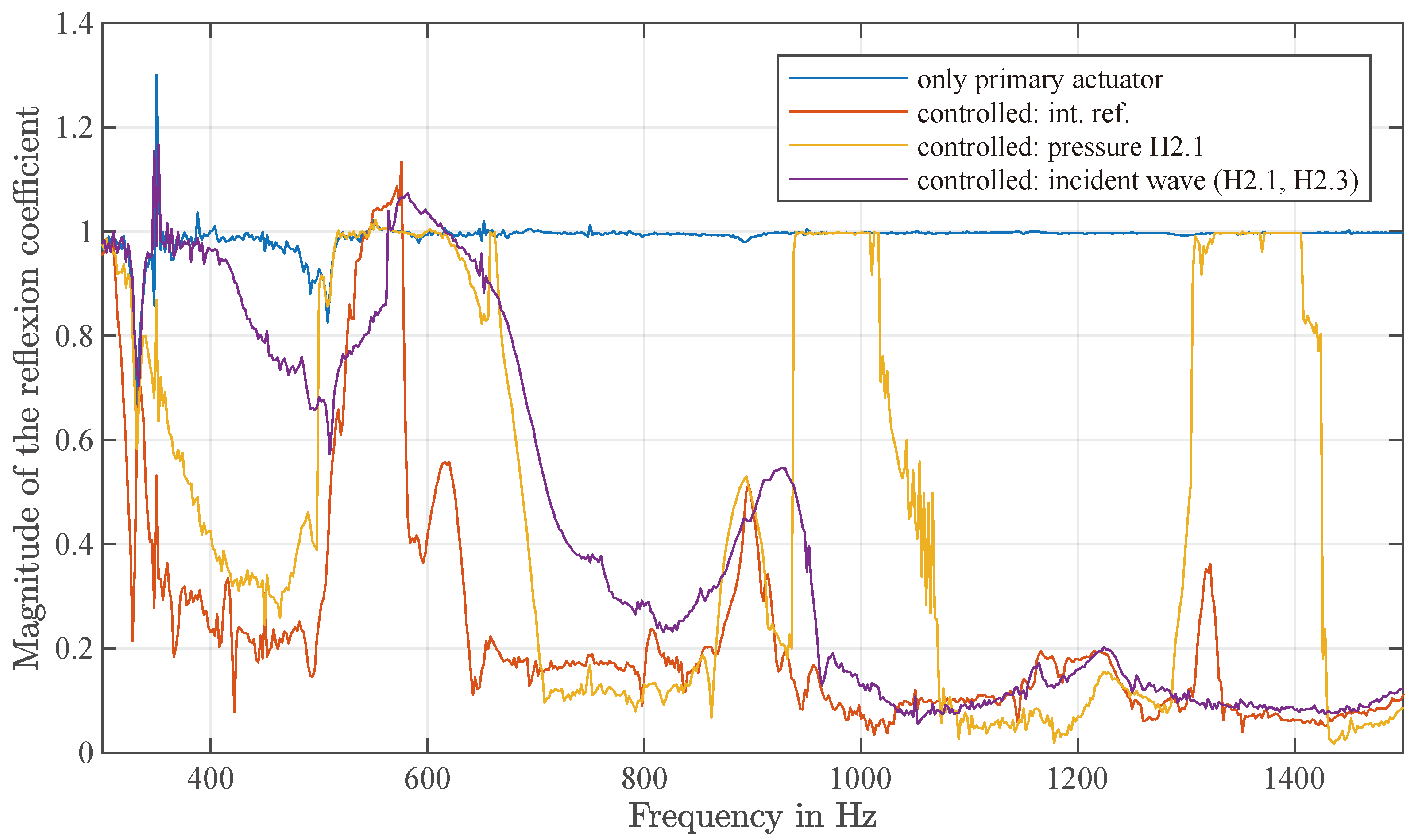
The SPL is a good indicator for the effectiveness of the active system. However, the reflection coefficient delivered more information because it shows the ratio of the incident and reflected wave directly. Figure 7 displays the magnitude of the reflection coefficient, calculated from H1.1 and H1.3, when applying a sine sweep from 300 Hz to 1500 Hz with $1.5\frac{\mathrm{Hz}}{\mathrm{s}}$.

The blue line represents the measurement without control. The magnitude of the reflection coefficient was slightly below one for most of the observed frequency range. This observation matches the assumption that the experimental piezo-actuator acts as a hard acoustic boundary condition. The red, yellow and purple lines represent the measurements with the three different reference signals. In a wide frequency range, the magnitude of the reflection coefficient can be reduced to approximately 0.1. All three implementations show better results for higher frequencies, which were probably caused by the higher signal-to-noise ratios (SNRs) of the signals. Preparatory measurements showed that the background noise below 500 Hz was high (spikes of up to 90 dB SPL in the spectrum and a floor of 65 dB), compared to the measured SPL in Figure 5 and Figure 6. The controller based on the internal reference struggled, in particular, at three multiples of the resonance frequency (586 Hz, 879 Hz and 1317 Hz). The controller with the pressure-based reference signal caused problems when the signal at H2.3 was low (see Figure 5, Top). The critical frequency ranges were 500 Hz–700 Hz, 950 Hz–1050 Hz and 1300 Hz to 1425 Hz. This result is in line with the observations in Figure 6 (Middle). The performance of the system with the wave separation reference was not as good as the other designs under 950 Hz. But, above this frequency, the system with wave separation performed better compared to the system with pressure as a reference signal. Contrary to our expectations, it even outperformed the internal reference design at an eigenfrequency of 1317 Hz. It achieved a reflection coefficient of 0.1 compared to 0.35.

The active system, independent of the reference signal used, was less effective below 500 Hz. It should be noted that the SNR at these frequencies was worse, since the actuators were less efficient in that frequency range and there was a significant amount of low frequency noise present in the signals. Unfortunately, the driving voltage of the experimental piezoceramic had to be limited to 25 V in order to minimize the risk of damaging the actuator. In addition, multiples of the mains frequency of 50 Hz had a negative impact on this experiment. This can be observed in Figure 7 at 350 Hz, where the reflection coefficient was overestimated. The magnitude of the reflection coefficient also showed local maxima at 450 Hz, 650 Hz and 750 Hz in the experiments.

4. Conclusions

The aim of this study was to develop an adaptive mechatronic system to reduce the reflections of sound waves from a submerged surface. For this purpose, an experimental setup with a water-filled tube, two actuators and multiple sensors was developed. Using acoustic wave separation and an FxLMS algorithm implemented on an FPGA-platform, an active system was presented that is able to control the wall impedance and, consequently, minimize the reflections of the surface. The results of the laboratory experiments with a water-filled impedance tube showed the high overall effectiveness of the system. Reflections at the active surface were significantly reduced in laboratory tests. The magnitude of the reflection coefficient below 0.1 in relevant frequency areas and the normalization of the pressure inside the tube both demonstrated the system’s effectiveness. The outstanding features of this system are the thin actuator (0.2 mm), the low latency of the FPGA-based implementation and the short distance of the reference sensors to the active surface (under 2 m). The instabilities of the adaptive controller can be explained by the physical properties of the measurement setup, such as its resonance effects. For applications in the open ocean, these resonance effects will not appear. Based on the findings in this paper, the implementation of such a system for an underwater vehicle is promising. In future studies, an array of piezo-actuators should be designed and tested for applications in larger structures. This requires an expansion into a multiple-input multiple-output configuration to accommodate the increased complexity introduced by actuator and sensor arrays.

References

1. Sachau, D.; Jukkert, S.; Hövelmann, N. Development and experimental verification of a robust active noise control system for a diesel engine in submarines. J. Sound Vib. 2016, 375, 1–18. [Google Scholar] [CrossRef]
2. D’Amico, A.; Pittenger, R. A brief history of active sonar. Aquat. Mamm. 2009, 35, 426–434. [Google Scholar] [CrossRef]
3. Cox, H. Fundamentals of the Bistatic Active Sonar. In Underwater Acoustic Data Processing, NATO ASI Series 161; Springer: Dordrecht, The Netherlands, 1989; pp. 3–24. [Google Scholar] [CrossRef]
4. Tyler, G.D. Low-Frequency Acoustics as an Antisubmarine Warfare. Johns Hopkins Apl Tech. Dig. 1992, 13, 145–159. [Google Scholar]
5. Sathish, K.; Anbazhagan, R.; Venkata, R.C.; Arena, F.; Pau, G. Investigation and Numerical Simulation of the Acoustic Target Strength of the Underwater Submarine Vehicle. Inventions 2022, 7, 111. [Google Scholar] [CrossRef]
6. Nolte, B.; Ehrlich, J.; Hofmann, H.G.; Schäfer, I.; Schäfke, A.; Stoltenberg, A.; Burgschweiger, R. Numerical Methods in Underwater Acoustics-Sound Propagation and Backscattering. Hydroacoustics 2015, 18, 127–140. [Google Scholar]
7. Fang, Y.Y.; Cheng, K.A.; Sung, P.J.; Chao, C.H.; Chen, C.F. Study of target strength of underwater vehicle. In Proceedings of the 2017 IEEE Underwater Technology (UT), Busan, Republic of Korea, 21–24 February 2017; pp. 1–5. [Google Scholar] [CrossRef]
8. Kwon, H.W.; Hong, S.Y.; Song, J.H. A Study for Acoustic Target Strength Characteristics of Submarines Using Kirchhoff Approximation. Mar. Technol. Soc. J. 2017, 51, 52–58. [Google Scholar] [CrossRef]
9. Avsic, T. An underwater vehicle shape with reduced acoustic backscatter. In Proceedings of the 23rd International Congress on Acoustics, Aachen, Germany, 9–13 September 2019; pp. 1935–1942. [Google Scholar]
10. Avsic, T. Stealth-Technik für Unterwasserfahrzeuge. Doctoral Dissertation, Hamburg University of Technology, Hamburg, Germany, 2021. [Google Scholar] [CrossRef]
11. Guicking, D.; Karcher, K. Active impedance control for one-dimensional sound. J. Vib. Acoust. Trans. ASME 1984, 106, 393–396. [Google Scholar] [CrossRef]
12. Suzuki, C. A new method absorption acoustic of measuring normal of materials incident using sound characteristics tube. Acoust. Soc. Jpn. 1981, 3, 161–167. [Google Scholar] [CrossRef]
13. Lacour, O.; Galland, M.A.; Thenail, D. Preliminary experiments on noise reduction in cavities using active impedance changes. J. Sound Vib. 2000, 230, 69–99. [Google Scholar] [CrossRef]
14. Timmermann, J.; Avsic, T.; Sachau, D.; Martens, I. Aktive Reduzierung der Schallreflexion an Oberflächen in Wasser. In Proceedings of the Fortschritte der Akustik—DAGA 2021, Jahrestagung für Akustik, Wien, Austria, 15–18 August 2021; p. 47. [Google Scholar]
15. Kuo, S.M.; Morgan, D.R. Active Noise Control System: Algorithm and DSP Implementations; John Wiley & Sons, Inc.: New York, NY, USA, 1996. [Google Scholar]
16. Klemd, A.; Eckert, M.; Klauer, B.; Hanselka, J.; Sachau, D. A parameterizable feedback FXLMS architecture for FPGA platforms. In Proceedings of the ACM International Conference Proceeding Series, Nagasaki, Japan, 6–7 June 2019; pp. 1–4. [Google Scholar] [CrossRef]
17. Klemd, A.; Klauer, B.; Timmermann, J.; Sachau, D. A flexible multi-channel feedback FXLMS architecture for FPGA platforms. In Proceedings of the 2021 31st International Conference on Field-Programmable Logic and Applications, FPL 2021, Dresden, Germany, 30 August–3 September 2021; pp. 319–326. [Google Scholar] [CrossRef]
18. Sherman, C.H.; Butler, J.L. Transducers and Arrays for Underwater Sound; Springer: Berlin, Germany, 2007; pp. 1–610. [Google Scholar] [CrossRef]
Figure 1. Schematic of the laboratory setup for active impedance control in a water-filled pipe.
Acoustics 05 00065 g001
Figure 2. Contacted 0.2 mm piezoceramic disc (Left) embedded in acoustic compound with steel housing (Right).
Acoustics 05 00065 g002
Figure 3. Measurement module with three pressure sensors and termination module with experimental piezo-actuator.
Acoustics 05 00065 g003
Figure 4. Experimental setup of the modular steel tube including the measurement hardware.
Acoustics 05 00065 g004
Figure 5. Comparison of the SPL of the primary Tonpilz transducer (Top) and the secondary experimental piezoceramic (Bottom).
Acoustics 05 00065 g005
Figure 6. Comparison of the controlled SPL: internal reference from the signal generator (Top), pressure at H2.3 as reference (Middle), reference based on the wave separation (incident sound wave, H2.1 and H2.3) (Bottom).
Acoustics 05 00065 g006
Figure 7. Magnitude of the reflection coefficient of the active surface.
Acoustics 05 00065 g007