Article

Identification of Noise Sources in a Realistic Turbofan Rotor Using Large Eddy Simulation

by
Pavel Kholodov
*,† and
Stéphane Moreau
Département de Génie Mécanique, Université de Sherbrooke, Sherbrooke, QC J1K2R1, Canada
*
Author to whom correspondence should be addressed.
These authors contributed equally to this work.
Acoustics 2020, 2(3), 691-706; https://doi.org/10.3390/acoustics2030037
Submission received: 18 August 2020 / Revised: 14 September 2020 / Accepted: 18 September 2020 / Published: 22 September 2020
(This article belongs to the Special Issue Aeroacoustics of Turbomachines)

Abstract

:
Large Eddy Simulation is performed using the NASA Source Diagnostic Test turbofan at approach conditions (62% of the design speed). The simulation is performed in a periodic domain containing one fan blade (rotor-alone configuration). The aerodynamic and acoustic results are compared with experimental data. The dilatation field and the dynamic mode decomposition (DMD) are employed to reveal the noise sources around the rotor. The trailing-edge radiation is effective starting from 50% of span. The strongest DMD modes come from the tip region. Two major noise contributors are shown, the first being the tip noise and the second being the trailing-edge noise. The Ffowcs Williams and Hawkings’ (FWH) analogy is used to compute the far-field noise from the solid surface of the blade. The analogy is computed for the full blade, for its tip region (outer 20% of span) and for lower 80% of span to see the contribution of the latter. The acoustics spectrum below 6 kHz is dominated by the tip part (tip noise), whereas the rest of the blade (trailing-edge noise) contributes more beyond that frequency.

1. Introduction

The latest noise standards imposed by International Civil Aviation Organization (ICAO) [1] have further restricted the maximum noise level for an aircraft certified after 2018. In the present generation of aircraft, the turbofan is already a major noise contributor in high bypass-ratio (HBR) aircraft engines [2,3,4,5] and in the overall aircraft noise as well (mostly in the forward arc and at approach). Moreover, as shown in [4,5], the importance of fan noise will only increase with the next generation of ultra-high bypass ratio (UHBR) engines at all certification flight conditions. Consequently, a further reduction of aircraft noise will require to predict and mitigate all fan noise sources. Currently, the main fan noise sources are the rotor–stator interaction (RSI) and the group of sources associated with the rotor blade: the turbulence interaction with the rotor blades, the trailing-edge turbulent boundary layer and the tip vortices [4,5]. Whereas the first one is the most important source in the HBR [2,3,4], the rotor noise sources will compete with it due to the geometric changes in the UHBR: the increased fan blade height and chord length, the decrease of the nacelle length and the shortened distance between the rotor and the outlet guide vanes.
Despite a number of remaining uncertainties, the numerical simulation allows studying these noise sources in realistic configurations [6,7,8] by resolving the flow field numerically and either computing directly or modeling the corresponding noise contributions [4]. Only a few numerical studies are devoted to the fan broadband noise. Most of them are carried out on the NASA Source Diagnostic Test (SDT) database [9,10,11,12] as it provides unique measurements for the aerodynamic and acoustic performance of a conventional HBR.
The rotor–stator interaction noise is generated by the interaction between the turbulent wakes of the rotor and the outlet guide vanes (OGV). This is currently the most studied noise source as the rotor wakes can be well resolved by using various numerical methods. The hybrid Lattice–Boltzmann Method (LBM)–Very Large Eddy Simulation (VLES) [13,14] and the hybrid unsteady Reynolds-Averaged Navier–Stokes (uRANS)–LES [15,16] computations give a reliable prediction of the RSI noise, as it may not require such a high grid resolution around the rotor blades. However, applied to the rotor noise prediction, these methods either require a near-wall mesh resolution that is too expensive (LBM) or do not resolve the near-wall turbulence at all (uRANS). Large Eddy Simulation (LES) is more suitable to study the flow around the rotor. The wall-modeled LES resolves most of the turbulence spectrum in combination with a wall function to predict the wall shear stress. It is capable to resolve the turbulent structures that may serve as effective rotor noise sources. The present study aims at decomposing and identifying these sources using the high-fidelity data obtained from rotor-only (RO) LES computations [8,17,18,19]. The focus is put on the approach operating condition (62% of the operating point rotation speed), for which the fan is the dominant contributor in the overall turbofan noise [2]. The previous studies showed that the modeling of the trailing-edge and turbulence-interaction noise sources is not enough to correctly predict the total rotor broadband noise spectrum [17,18]. The analysis of the flow field showed that a complex tip flow, interacting with the neighbouring blades, can be an additional noise source along with the described two sources [8,19]. The current study aims at providing a deeper understanding of these noise sources and their contribution to the overall rotor broadband noise.
The paper is organized as follows. Section 2 describes the numerical model. Section 3 shows the aerodynamic results and their validation against experimental data. Then, the dynamic mode decomposition is shown to identify the possible noise sources around the rotor. Section 4 discusses the noise prediction from the rotor blade surface. Finally, conclusions are drawn.

2. Numerical Model

The present study simulates the RO configuration of the NASA SDT benchmark using the wall-modeled LES methodology. The geometry of the domain is shown in Figure 1. The domain is fully embedded inside the nacelle geometry and represents the external contour of a typical HBR turbofan. The rotor is simulated with periodic boundary conditions applied on the lateral surfaces of the sector. One rotor blade is computed. The hybrid computational grid is based on previous computations made for the Rotor–Stator configuration [20]. It consists of 62 million elements with 8 prism layers on the rotor blade such that the maximum dimensionless distance to the wall is Y + ∼30. The grid near the hub and casing surfaces is made without prism layers. The grid statistics is given in Table 1, the slice of the grid is presented in Figure 2.
The code AVBP [21] is used for the compressible LES. It has been extensively validated against multiple turbomachinery cases, including both aerodynamic and aeroacoustic ones [6,7,20,22]. The Taylor–Galerkin scheme TTG4A [23] that is 3 rd order accurate in space and 4 th order in time is used. The inlet and outlet boundary conditions are set as non-reflecting Navier–Stokes characteristic boundary conditions. These boundary conditions are defined with relaxation factors towards the mean velocity (at the inlet) and the mean pressure (at the outlet). The mean profiles themselves are taken from the previously made RANS computations [17]. No turbulence is injected at the inlet. Classical wall functions are applied on the solid surfaces. The computation is initialized from previous simulations of the RO configuration (see Pérez Arroyo et al. [8,17]). It is further run for 1 revolution of the rotor to verify the proper flow establishment. The case is then continued for 7 more revolutions to collect the unsteady statistics.
The time step of the simulation is 1.2 · 10 8 s. The unsteady data are collected with the time interval of 7 · 10 6 s, which yields a Nyquist frequency of around 75 kHz.

3. Aerodynamic Results

3.1. Mean Flow

The comparison of the measured and computed aerodynamic performances with the experiments is shown in Table 2. The computation shows similar performance and slight difference in the mass-flow rate compared to the experiments.
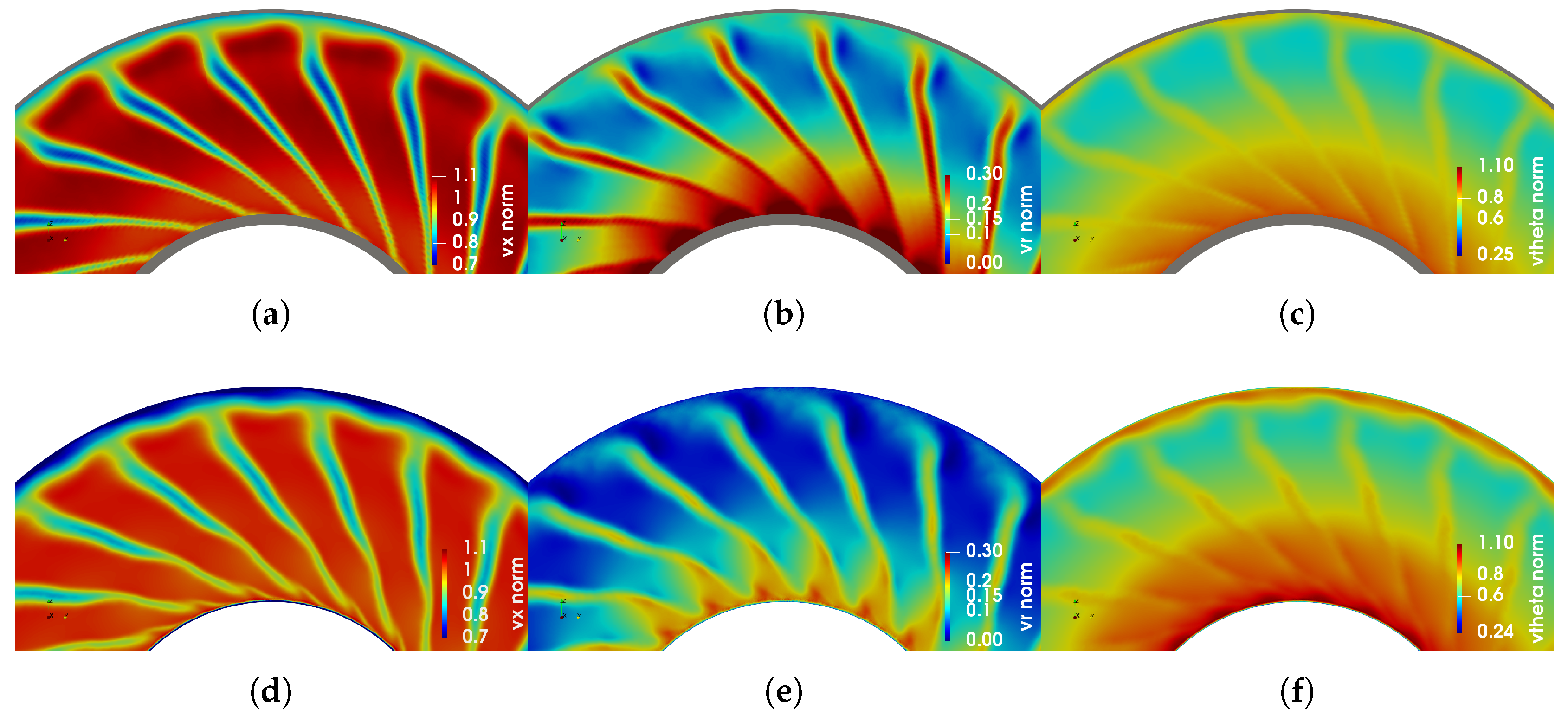
The contours of the mean velocity components at the mid-distance between the rotor and the theoretical stator location are presented in Figure 3 for LES and the experiment. Experimental data were obtained using Hot-Wire Anemometry (HWA) [24]. The velocities are normalized by the experimental mean axial velocity averaged in the measurement plane v ¯ x = 112.42 m/s. The results show that the wake width is well captured in LES. However, there exists some over-prediction in the tip zone, where the flow blockage is stronger than in the experiment. In addition to that, a notable difference exists in the radial component of the mean velocity that is higher in the experiment for the wake and the inter-wake region. For the experiment and LES, the axial velocity component dominates in the flow except for the lower 40% of span where the tangential component also becomes relatively large.
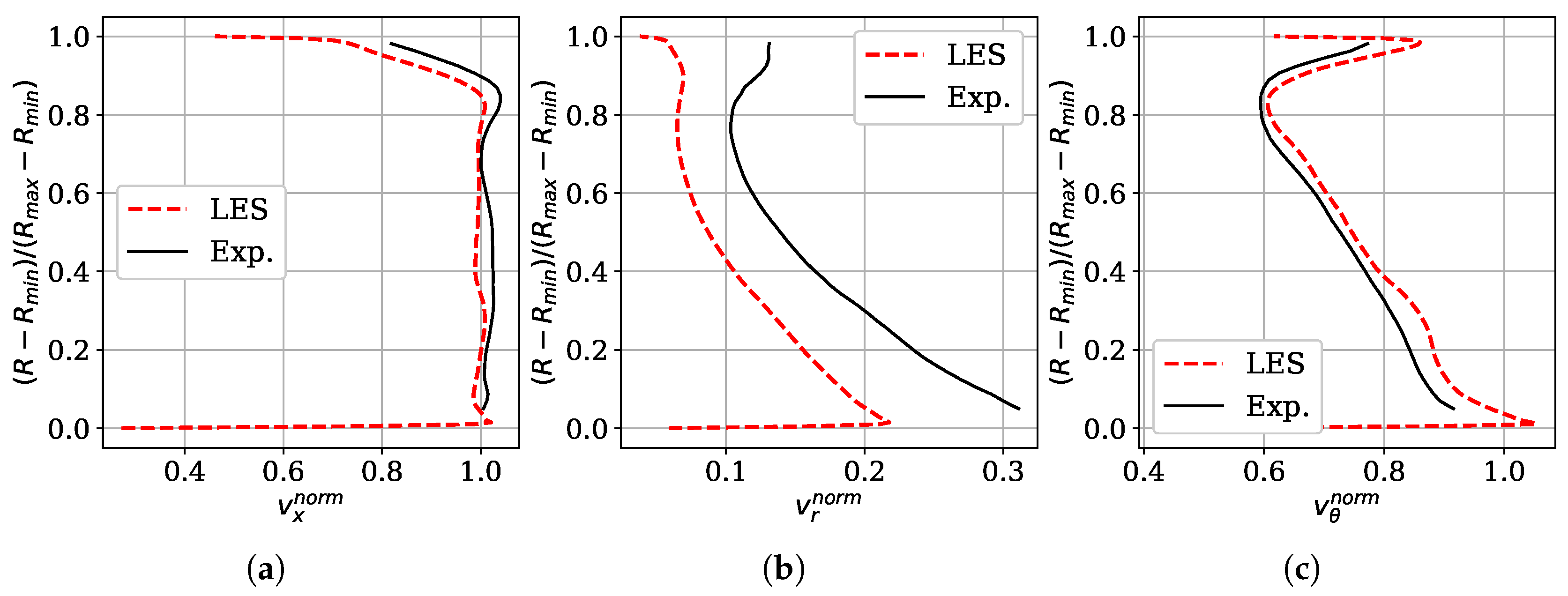
More quantitative comparison is given in form of meridional profiles at the same axial position. The results are presented in Figure 4. All the components are normalized by the same quantity as in Figure 3. This comparison shows that, except for the radial component, there is a very good match between the computation and experimental data. For the radial velocity component, the lower values in LES indicate a better radial equilibrium condition. It may be the effect of boundary profiles obtained from RANS simulations [17], where this condition was imposed on the outlet surface.
The relative difference between the profiles can be estimated by interpolating LES data on the experimental grid. By doing this, the obtained root mean square (RMS) of the difference between LES and the experiment is 3.6% for the axial, 6.4% for the radial and 3.7% for the tangential components. A notable difference between the computation and the experiment exists only in the region very close to the tip. There, the maximum difference reaches 0.092 v ¯ x in the axial velocity at 96% of span. For the radial velocity it is 0.11 v ¯ x at 5% of span. For the tangential velocity, the maximum difference is 0.086 v ¯ x at 98% of span. These span positions are on the edge of the casing boundary layer and are probably affected by the absence of the prism layers on the casing wall in LES. Consequently, the previously stated difference in the mass-flow rate comes from stronger flow blockage in the very tip of the flow passage.
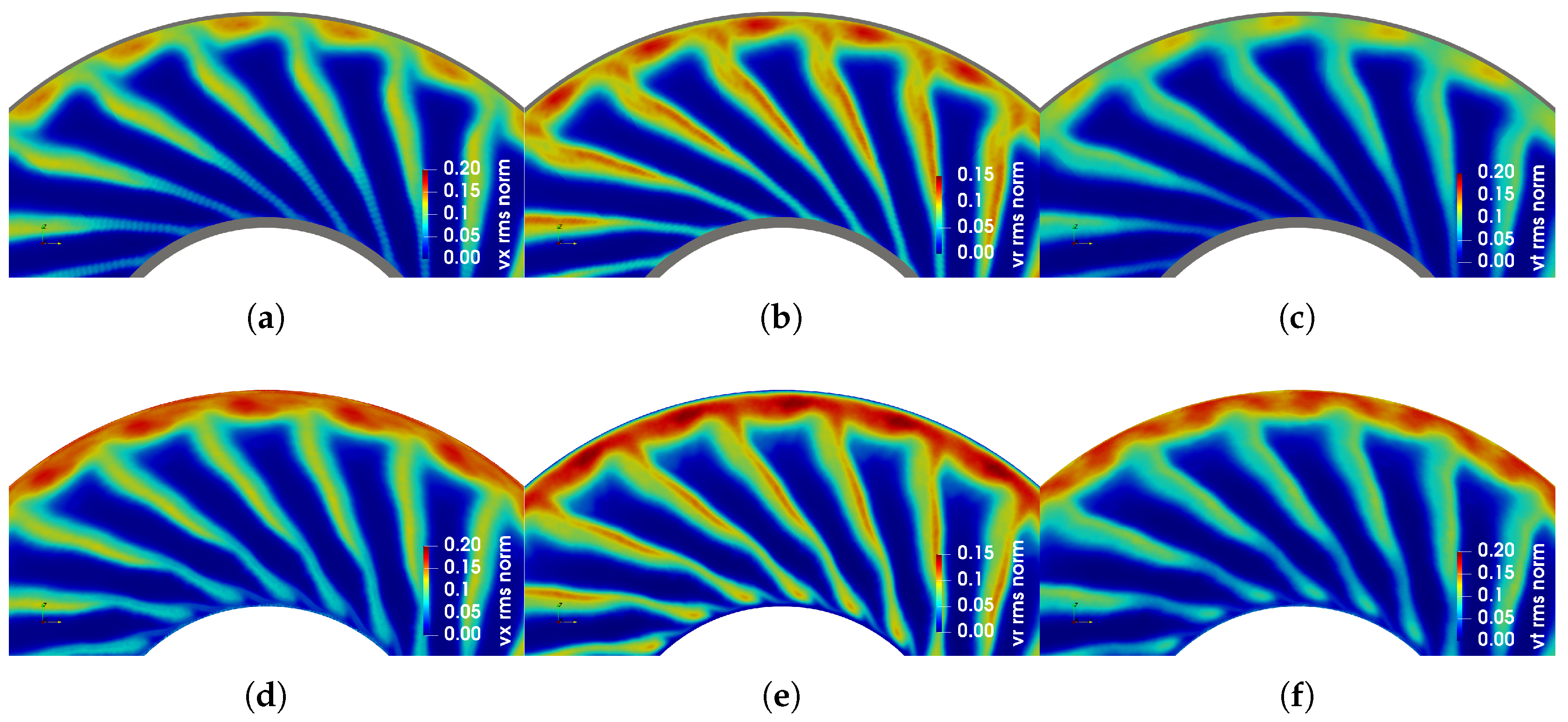
The normalized RMS contours of the velocity fluctuations are shown in Figure 5 for the same axial position as the mean velocities. Again, there is a good match with experimental data. The RMS values in the wake are close to the experiment, and an over-prediction exists only in the tip region. There is also a spot of elevated RMS values close to the hub in LES which is possibly a trace of the corner vortex. The maximum RMS values of the axial velocity fluctuations are located in the middle of the wake, whereas the radial and tangential components have their maxima shifted to one side.
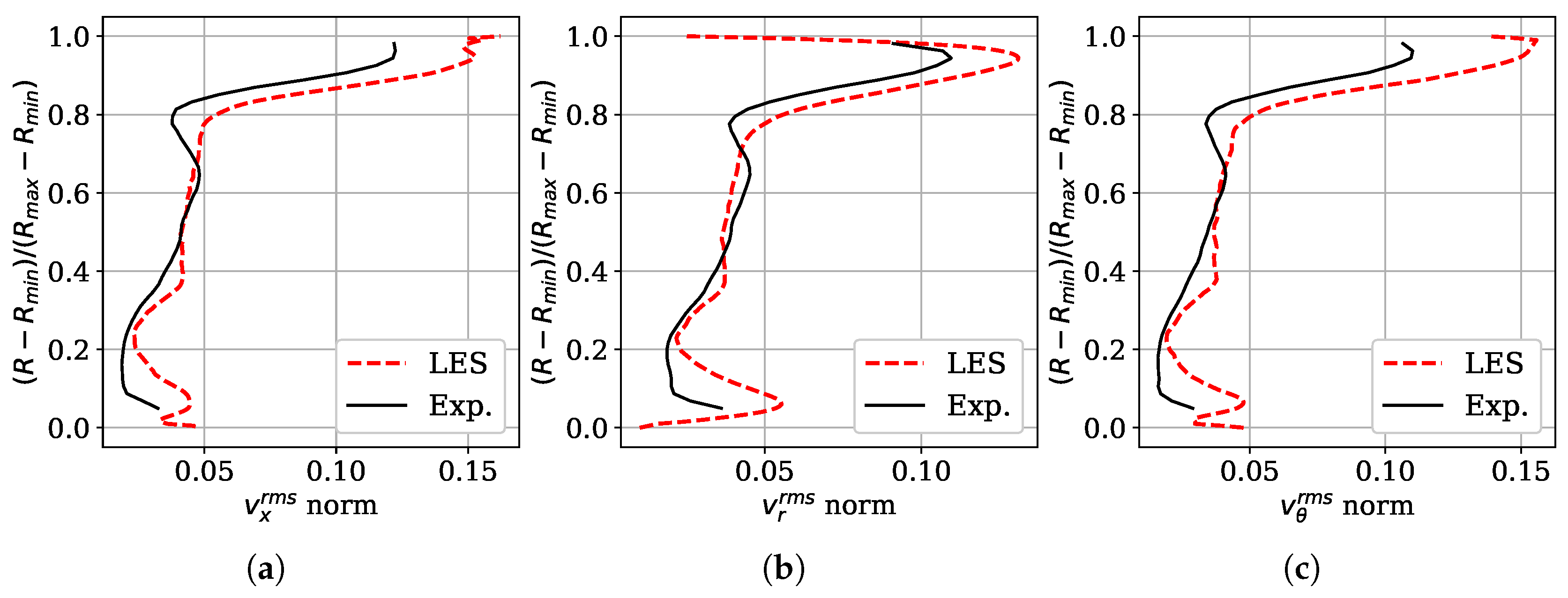
The same procedure as for the mean velocities is applied to estimate the difference between LES and the experiment. The RMS of the difference between computed and measured data is 1.5% for the axial, 1.2% for the radial and 1.7% for the tangential components. The meridional profiles shown in Figure 6 depict a close match between 20% and 80% of span. After 80%, the difference is present for all three components. The maximum difference between the profiles is 0.048 v ¯ x for the axial, 0.034 v ¯ x for the radial and 0.029 v ¯ x for the tangential component. Interestingly, all three components have the same position of the maximum difference with the experiments which is 89% of span. The profiles also show a growing trend in experimental data below 10% of span that possibly corresponds to the corner vortex. The corresponding growth of all three RMS components in LES starts below 20% of span.
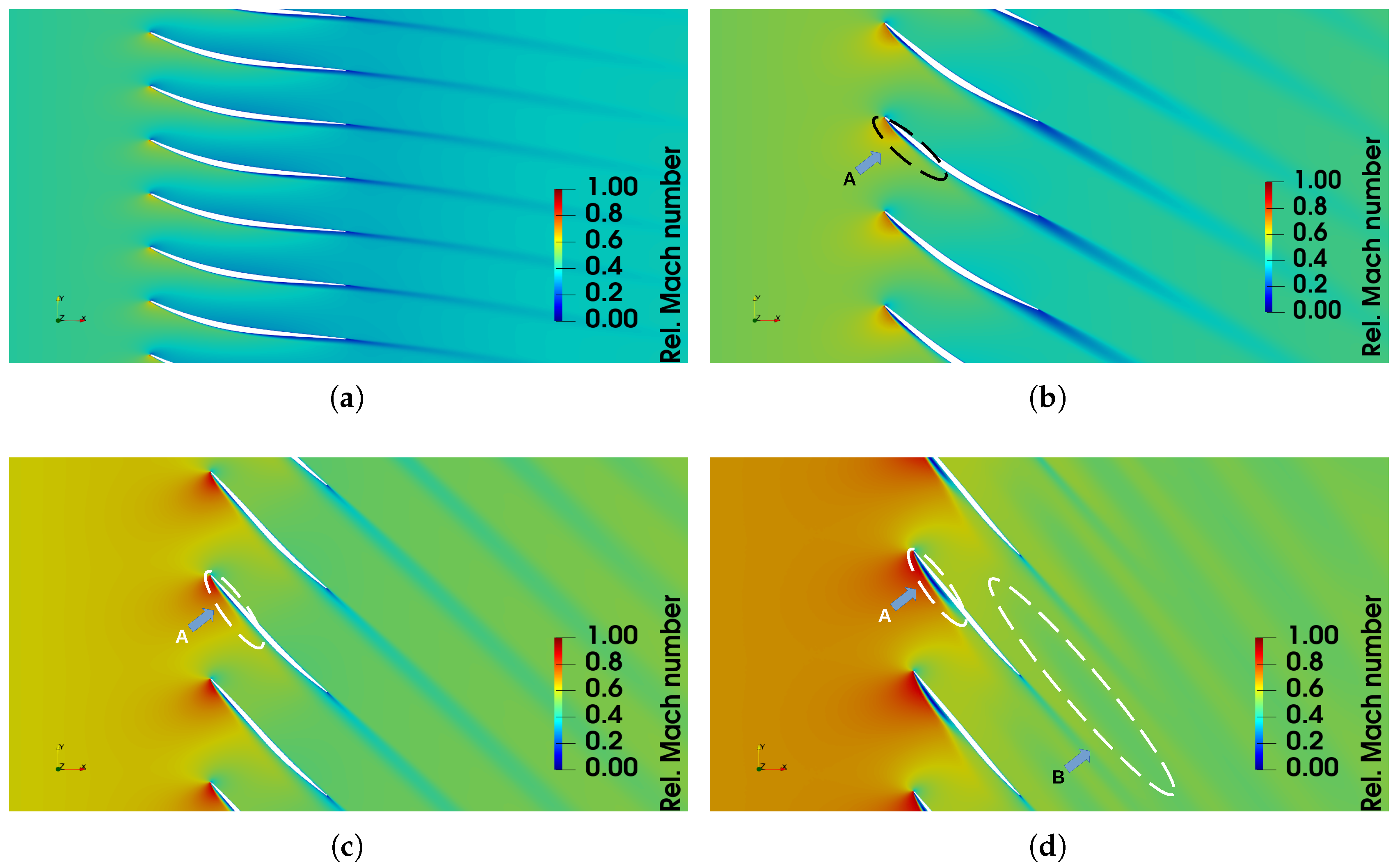
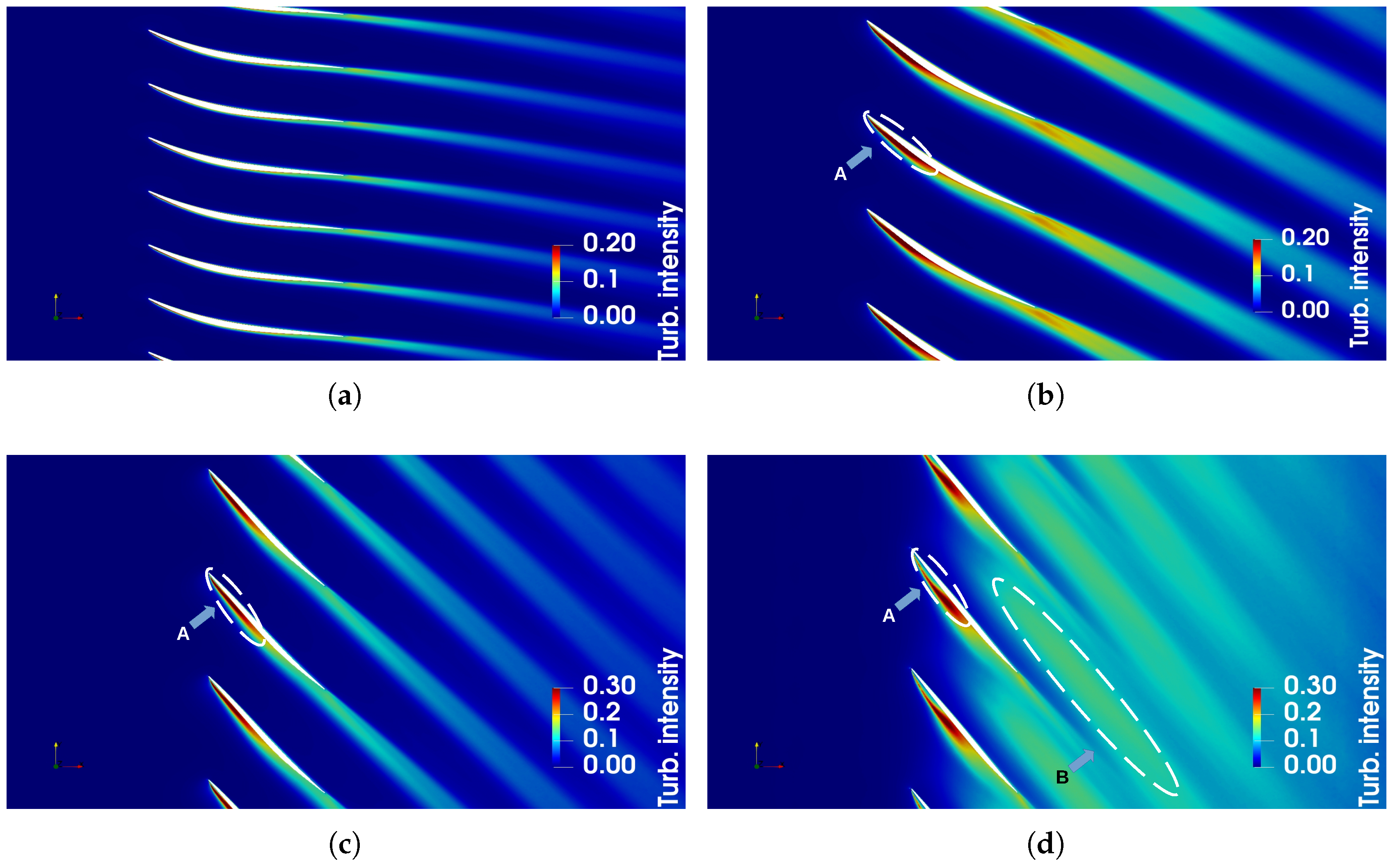
The results presented above show that, despite some over-prediction in the outer part of the flow passage the LES computation is quite close to the experiments. This allows studying further the mean flow field in the rest of the domain. The relative Mach number contours and the turbulence intensity at different spanwise positions are presented in Figure 7 and Figure 8. The flow field does not reveal any particularity at 25% of span. A leading-edge flow detachment is visible by low-Mach number and high turbulence intensity zones on the suction side at 50% of span (zone A). The detachment grows with the increase in span. The unsteady flow analysis presented below will show that it is a trace of a spanwise-moving leading-edge vortex. At 90%, the separation zone occupies one half of the suction side and is associated with the high-level zone of turbulence intensity. At this spanwise position, the leading-edge vortex rolls off towards the trailing edge and collides with the lowermost part of the tip vortices. A low-velocity and high-turbulence zone (B) is also visible in the inter-blade region. It is an averaged trace of tip vortices that are moving streamwise and inwards while being convected by the mean flow.

3.2. Unsteady Flow

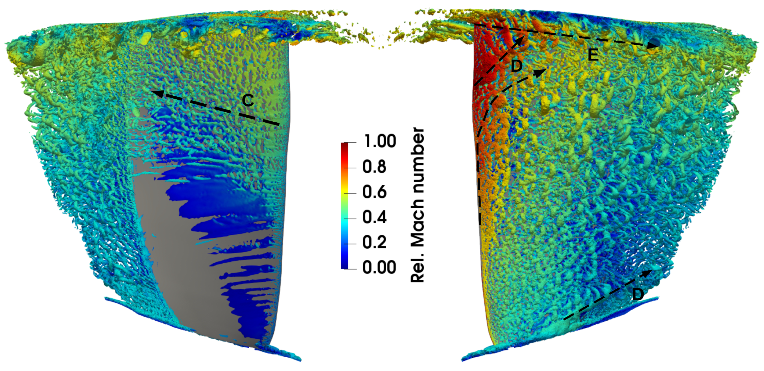
The next step in the study is to investigate the unsteady flow pattern in order to reveal the flow features that can possibly serve as noise excitation mechanisms. The unsteady flow is visualized in the form of iso-surfaces of the Q-criterion in Figure 9. The pressure side of the rotor blade does not reveal any turbulent structures up to 50% of span. Further outwards, only a few small-scale structures are visible. They are convected towards the trailing edge of the blade (C). On the suction side the flow is highly turbulent. The leading-edge vortex is moving radially outwards under the effect of centrifugal force and blade twist (D). The collision of this vortex with the tip vortices (zone E) is clearly seen in Figure 7 and Figure 8d (zone A). Moreover, the tip vortices plunge while moving in the streamwise direction to appear in the same figures (zone B). The other noticeable feature is the corner vortex (Figure 9 (right), zone D) that leaves its trace below 20% of span in the mean flow of Figure 3, Figure 4, Figure 5 and Figure 6. Its outward movement explains the increased radial component of the velocity in those figures.
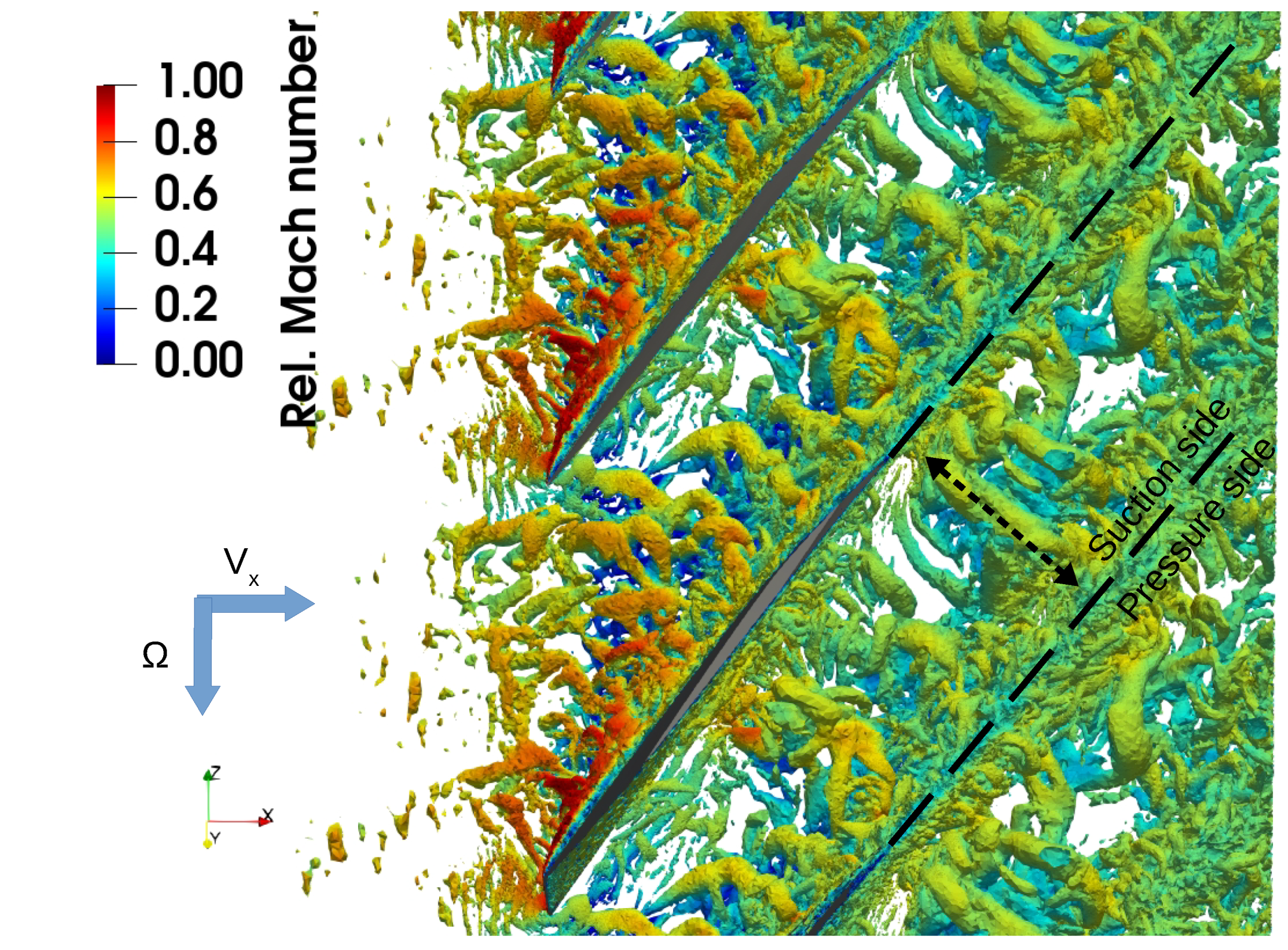
The view from the hub on the tip vortices highlights their evolution with the flow (Figure 10). This view reveals the formation of large tube-like structures moving between the blades. Some of them have the transverse length scale that is almost equal to the distance between the blades (dotted arrow). These structures evolve from the zone E in Figure 9.
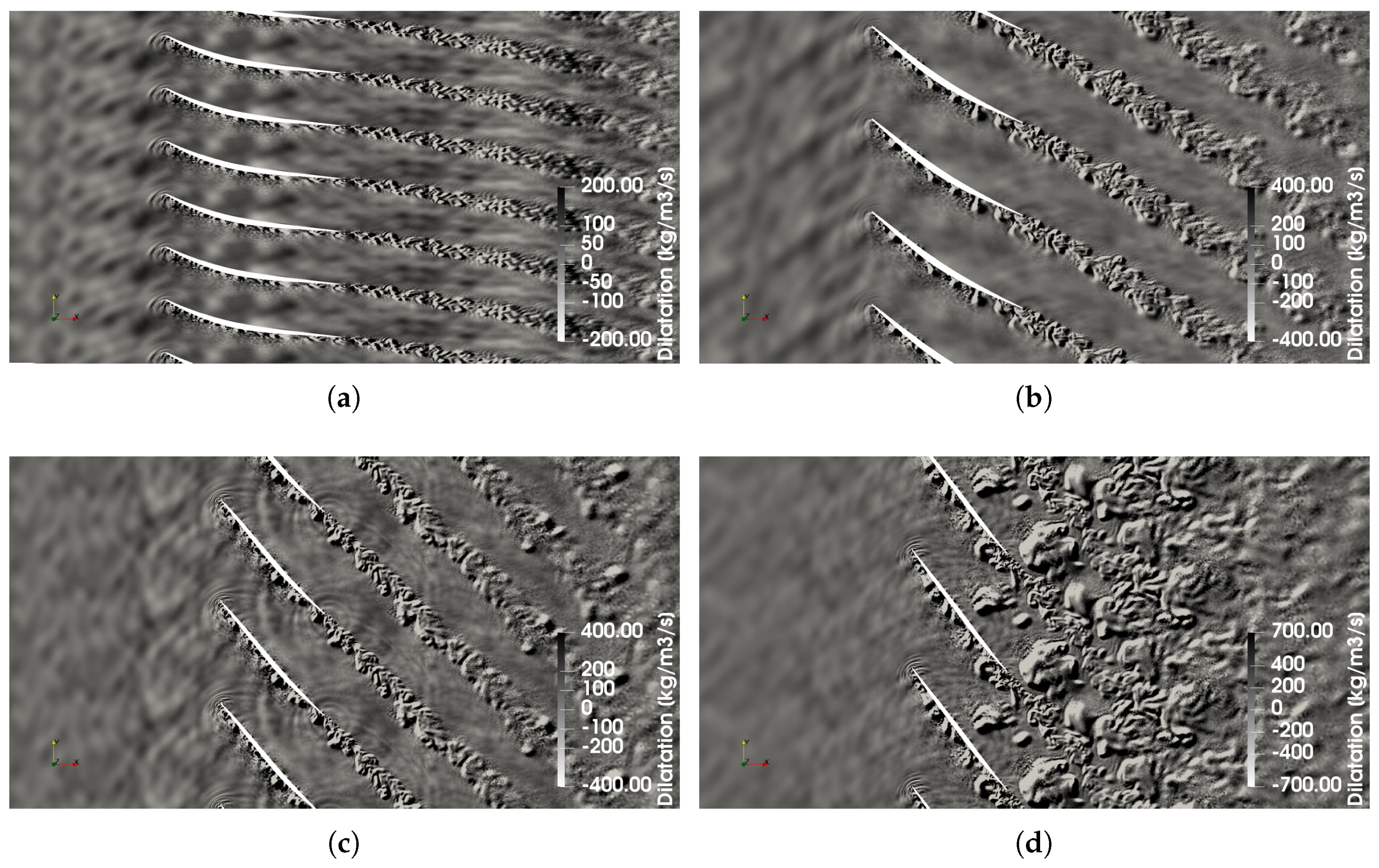
The dilatation field ( ρ / t ) allows identifying the flow perturbations that can serve as noise excitation mechanisms. Snapshots of four blade-to-blade views (in the rotor-locked reference frame) at different span positions are given in Figure 11. The common behavior for all presented positions is a clean flow upstream of the rotor. At 25% of span only the rotor wakes are presented as a source of flow disturbance. However, low-amplitude patterns everywhere in the inter-blade region and upstream reveal an intensive propagation of the acoustic-scale waves. The circular patterns visible around the leading edge is a diffraction of these waves. The animated dilatation field shows the dynamics of the diffraction of the acoustic waves as they leave the inter-blade region and propagate further upstream.
At 50% and 75% of span, the turbulent wakes of the rotor become wider and stronger. In-between the wakes, the flow is still as clean as upstream of the fan. The wakes mainly originate from the turbulent boundary layer on the suction side of the blade, whereas the pressure-side flow is almost quiescent at 50% and shows only small-scale perturbations at 75% of span. They likely come from the small structures in Figure 9 (left). At 90% of span, the other source of large-scale perturbations appears in the inter-blade region, completely disturbing the flow field downstream of the rotor. This phenomenon is the trace of the tip vortices grazing along the blade surface (Figure 9 (right), zone E).
Starting from 50% of span, there are circular wave patterns coming from the trailing edge. These acoustic waves are believed to be the source of the wave propagating upstream and visible at all span positions. They also move downstream; their reflection from the turbulent wakes and the interference between neighboring sources is clearly visible at 75%. The strength of the trailing-edge sources apparently grows with increasing spanwise location (and the local flow velocity). Nevertheless, they are hidden under the tip vortices appearing at 90% between the wakes. Still, the wave diffraction is present at this spanwise position and is expectedly stronger than at 75% of span. These vortices are likely to emit acoustic waves themselves along with the trailing-edge source. This is assessed by the modal analysis presented in the next section, and the far-field acoustics computation presented later in the paper.

3.3. Dynamic Mode Decomposition

The dynamic mode decomposition (DMD) [25] is computed using the unsteady pressure field upstream and downstream of the rotor. Two volumes are used for the recording, each is 0.12 m length and occupies all the radial and azimuthal extents of the domain. The length of the volume is chosen to fully contain one wavelength of the acoustic wave propagating at the first blade passing frequency (BPF), 2863 Hz. The volumes are shown in Figure 12.
A total of 4096 snapshots are used for the decomposition. The data are recorded with a sampling frequency of 75 kHz and interpolated on a regular mesh with a cell size of 0.002 m. Then, a dynamic mode decomposition [25] is performed in the stationary reference frame for each volume using the python library Antares developed at CERFACS, France [26]. The discrete pressure field is decomposed on an ensemble of DMD modes:
p k x n = A k p 0 x n = i λ i k Φ i x n
where p k is a k-th snapshot value of the pressure field, A k is a linear mapping operator, λ i k is an eigenvalue, Φ i x n is a DMD mode.
The angular complex frequency of the DMD mode is obtained as:
ω i = ln λ i Δ t
where Δ t is the recording time step. The modal amplitude is obtained by taking a quadratic norm of the DMD mode scaled by the cell volumes to obtain physically meaningful quantities:
Φ i = Φ i * Φ i ( N 1 ) V c
where N is the number of snapshots and V c is the cell volume.
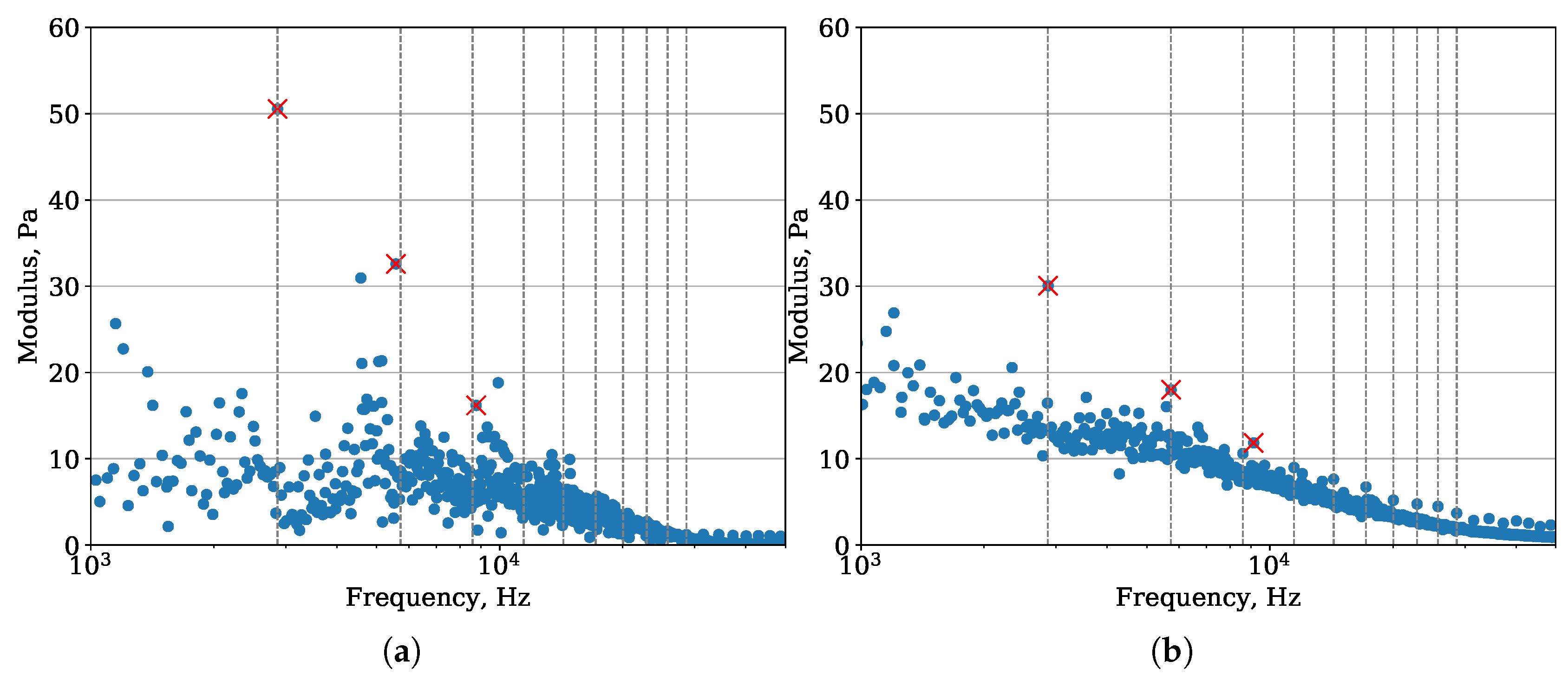
As a result, the amplitude spectra are given in Figure 13 for the upstream and downstream volumes. The spectra allow identifying the most energetic modes and segregating particular modes around the frequencies of interest. In both spectra such modes are present around the first three BPF and are highlighted by the red crosses in the figure. The most prominent are the modes at the first BPF: for the upstream volume, the difference between the mean spectrum level and this mode is more than 40 Pa. For the downstream volume, this difference is smaller and counts 15 Pa. In general, the downstream spectrum is more smooth, most probably due to the presence of the strong hydrodynamic fluctuations coming from the wakes and having the same order of magnitude, whereas the clean upstream flow exhibits mostly the acoustic waves upon the quiet environment, as seen in Figure 11. The other notable feature of the spectra is a sub-harmonic hump slightly below the second BPF in the upstream spectrum.
The temporal reconstruction of the DMD modes is obtained from the amplitude and the phase:
p i ( x n , t ) = Φ i cos 2 π t T + ϕ i
where t is the time, T = 1 / f i is the period of the fluctuations ( f i = ω i / 2 π ), Φ i is the amplitude and ϕ i is the phase of the DMD mode i.
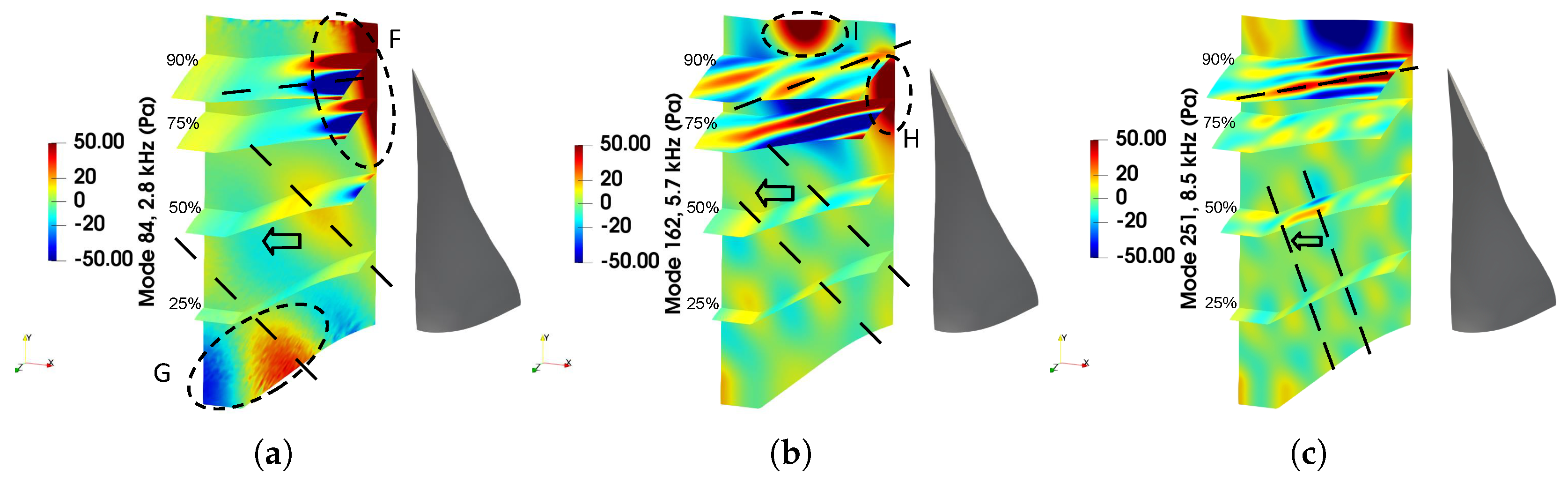
The reconstruction of the upstream volume is shown in Figure 14. It should be noted that all the modes are moving in all three directions, the dominant being the azimuthal (the rotation direction) and the axial ones. The mode at BPF1 (2.8 kHz) originates from the upper part of the blade. The amplitude of the mode increases from 50% of span and up to the tip (zone F). This corresponds very well to the diffraction patterns visible from the same spanwise position in Figure 11. The amplitude of the mode quickly decays; however, the mode is not evanescent as it continues to propagate farther upstream with a smaller amplitude. Close to the hub, where the annular duct swiftly changes to the cylindrical one (zone G), the amplitude suddenly increases, which is the evidence of the mode matching between these two duct shapes. The inclination of the wave front suggests that even at low spanwise locations the waves come from the tip region.
The second mode, located almost exactly at BPF2 (5.7 kHz), shows different pattern. It is also the strongest at the tip, where it contains two lobes (zones H and I): the first one coming from around 75–80% of span and the second one located directly at the tip. When combined with the plots of the dilatation and the Q-criterion this mode can be assumed to originate from the roll-off of the leading-edge vortex (zone D in Figure 9) and the tip vortices (zone B in Figure 8, zone E in Figure 9). At lower blade height, the inclination of the wave front is almost the same as in the mode at BPF1. This shows that the tip region is still a dominant source of acoustic waves at this frequency. The third upstream mode analyzed in the paper lies at 8.5 kHz (BPF3). Its maximum of amplitude still resides at the tip. Nevertheless, the acoustic wave propagates at a larger angle with respect to the fan axis. It exhibits an increased role of the other noise source at this frequency such as the trailing-edge noise. Other than that, the character of this mode is similar to the previously described ones.
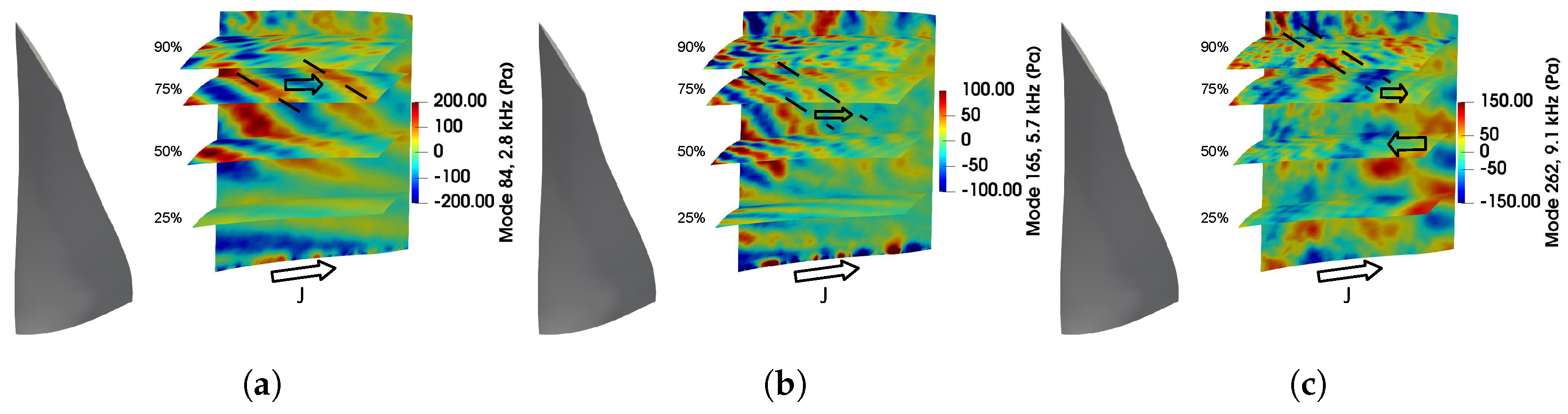
A similar analysis is applied to the modes in the downstream volume which are shown in Figure 15. Here, the first considered mode at 2.8 kHz is dominated by the fan wakes. At this frequency the hydrodynamic perturbations are masking the acoustic pressure field, and for most of the span the acoustic patterns are hardly distinguishable. However, below 30% height, the wakes become weaker and more axially aligned, and the temporal reconstruction shows almost axial propagation near the stationary part of the hub (zone J). It is obviously linked to the lower stagger angle of the fan blades and the smaller rotational speed. The second mode at 5.7 kHz (BPF2) shows larger amplitudes in the tip region (above 90% of span). It is coherent with the upstream mode at the same frequency (Figure 14b) that also has a high amplitude in the same spanwise region.
The third downstream mode propagates at 9.1 kHz which is higher than BPF3 (8.5 kHz). It is only a couple of Pa higher than the mean level of the DMD modes at this frequency. However, this mode is interesting to consider because of its complex propagation behavior. In the outer half of the flow passage the mode propagates similarly to the modes at BPF1 and BPF2. Below 50%, the axial propagation direction changes and the animated reconstruction reveals that the waves move upstream. Finally, very close to the hub, similar to the modes at BPF1 and BPF2, the propagation direction again changes to downstream. The upstream propagation of the mode at span below 50% matches well with the same observation made upon the dilatation field.
Making preliminary conclusions, the modal analysis shows that, in the low and mid-frequency range, most of the acoustic fluctuations come from the tip region of the blade. It is particularly visible in the upstream volume, where the flow is not contaminated by the hydrodynamic fluctuations. For higher frequencies, the trailing-edge noise starts to make its contribution to the noise propagation as well. The following section assesses how this near-field analysis corresponds to the far-field acoustics prediction.

4. Acoustic Results

For the acoustics computation, the unsteady pressure field is recorded on the solid surface of the fan blade. The sampling frequency is the same as for the DMD study, namely 75 kHz. The recording is made for 7 rotor revolutions. The far-field acoustics computation is made with the Ffowcs Williams and Hawkings’ analogy (FWH). The formulations of Casalino [27] and Najafi-Yazdi [28] had been implemented in the in-house code SherFWH. The loading-noise source term is computed integrating over the blade surface and the acoustics propagation is computed using the free-field Green’s function. A free-field axial Mach number of 0.1 is also accounted for to match wind-tunnel conditions. The far-field sound power level spectrum is obtained using Welch’s method and Hann windows with 50% overlap.
Along with the prediction for the whole blade surface, the computation is made for the blade split on two parts. The outer 20% of the blade is taken to investigate the contribution that is made by the tip flow to the far-field acoustics. The size of this part is chosen according to the results from the previous sections which show that this region is largely dominated by the tip flow. Moreover, the previous section also suggests that the major acoustic perturbations come from this part of the blade. The full power spectral density of the far-field acoustic pressure can be represented as the sum of the power spectral densities of the corresponding parts and their cross-spectral density:
p ^ p ^ b l a d e = p ^ p ^ t i p + p ^ p ^ l o w + p ^ t i p p ^ l o w
The results are shown in Figure 16 for the full blade, the two parts and the cross-correlation term for the upstream and the downstream propagation directions. The computed spectra give a good level of prediction with some over-predicted levels for the downstream direction in the mid-frequency range. The over-prediction of the computed spectrum is likely a consequence of the free-field Green’s function that neglects the effect of the annular duct downstream of the fan. The previous study [19] indirectly confirms it by the comparison of the experimental spectra with the spectra computed for permeable surfaces upstream and downstream of the rotor. Yet, the current analysis is useful in a sense that it allows identifying the blade regions contributing to the far-field noise. The tip part of the blade dominates the spectrum below 5.5 kHz. The difference between the tip and the low parts in this frequency range is around 5 dB. The hump appearing near the BPF1 in the upstream spectrum is clearly linked to the strong mode at the same frequency observed by DMD in the tip. Its presence in the far-field results can be likely explained by the formulation of the FWH analogy which does not take into account the decay of some acoustic modes in the near field which is the case in Figure 14a. The same happens with the hump around 1.2 kHz, which corresponds to peak modes in the DMD spectrum. The over-prediction at BPF2 is smaller and it matches well with the DMD results as the mode in Figure 14b clearly propagates farther than its counterpart at BPF1. A similar hump can also be noticed in the DMD upstream spectrum in Figure 13a. The low part of the blade becomes larger than the tip beyond 5.5 kHz and is dominant at BPF3 (8.5 kHz). It indirectly confirms the previous observation about the increased angle of the wave front in Figure 14c, which is attributed to the trailing-edge noise contribution. For the rest of the spectrum, the low part of the blade stays dominant.
The situation is similar for the downstream spectrum, except that the low part starts to contribute between BPF2 and BPF3. The low-frequency part of the spectrum is under-predicted. Yet, in the experiment, the contribution in this range is made by the jet noise and the impingement of the swirling wake on a supporting strut (see [10,11] for details). These additional noise sources are absent in the present simulation, which triggers the observed under-prediction. The hump in the full-blade spectrum below BPF2 still comes from the tip part. In fact, the tip-region spectrum depicts three humps of almost the same amplitude at 5.2, 7.1 and 10 kHz. In the high-frequency part of the spectrum, the tip and the low-part levels are roughly equal until 30 kHz, where the tip levels become higher. In general, the downstream direction is more difficult to analyze than the upstream one because of the hydrodynamic perturbations masking the acoustic modes. However, the acoustic spectra clearly show that the tip and the low parts of the blade act in the same frequency range for both propagation directions. Hence, one can suggest that these contributions come from the same sources on the blade. The cross-correlation spectrum for both directions is quite small and is not expected to contribute significantly in the whole frequency range. It matches well the previous observations, in particular the mean-flow meridional profiles (Figure 6), where the high levels of the velocity RMS fluctuations stay within the outer 20% of the span.

5. Conclusions

The LES computation performed for the rotor-alone configuration of the NASA Source Diagnostic Test benchmark at approach has allowed identifying different rotor noise sources. First of all, the results are extensively validated against the experimental measurements. The mean-flow profiles and contours showed a good match between LES and the experiments. The flow is slightly over-predicted near the tip region, where a stronger blockage is observed in the LES results. The radial equilibrium is better respected in LES, probably due to the imposed outlet pressure profile. For the axial and tangential velocity components, the flow closely matches the experiment below 80% of span.
The noise source identification was then made with the help of several techniques. The iso-contours of the dilatation field revealed sources of acoustics-scale perturbation that may serve as noise contributors. Starting from 50% of span, circular waves appear near the trailing-edge of the fan blade, which is the evidence of the trailing-edge noise. At 90% of span, the tip vortices appear in many scales and enhance the diffraction and the interference patterns of the unsteady perturbations.
The dynamic mode decomposition was then performed for the pressure upstream and downstream of the fan blade. It presented several strong modes around the first three blade passing frequencies. The temporal reconstruction of them showed that these modes originate from the tip region of the blade. However, around BPF3, the contribution from the rest of the blade becomes more evident. The conclusions on the modal behavior are easier to make for the upstream volume. The modal picture is strongly distorted downstream of the rotor and masked by the turbulent wakes of the rotor creating strong hydrodynamic fluctuations. Still, an interesting phenomenon was observed for the mode at BPF3, namely the upstream modal propagation below 50% of span. This observation matches very well with the analysis of the dilatation contours.
Finally, the acoustics computation was performed with the Ffowcs Williams and Hawkings’ analogy. The far-field spectra showed a good match with the experiment. Some over-prediction comes from the neglected effect of the annular duct on the sound propagation. The blade was also split into two regions: the outer 20% of the span and the rest. Such a splitting allowed showing that the tip part of the blade is a dominant contributor in the frequency range up to 5.5 kHz in the upstream and 6 kHz in the downstream directions. The cross-correlation spectrum between the tip and the rest of the blade is low in all the frequency range. Such a low level most likely results from the fact that the turbulent structures of the tip region stay within the outer 20% of span.
The provided analysis has identified the tip noise and the trailing-edge noise as the main sources of the fan broadband noise in the case of a clean inflow, each in its own frequency range, similarly to what was found previously for low-speed fans [29]. The current study showed that the combination of the detailed near-field analysis with the far-field acoustics computation can give many interesting insights on the noise generation and propagation in the fan. Still, more details of the noise propagation might be revealed by carrying out additional analysis in the future work. One of the perspective techniques might be the filtering of the downstream data by separating acoustic and hydrodynamic fluctuations. The impact of the duct on the noise propagation can be shown by projecting the recorded data on the duct modes. The modal and correlation analysis directly in the tip region of the blade can give more details on the orientation of the tip structures and their interaction with the blade.

Author Contributions

Conceptualization, P.K. and S.M.; methodology, P.K. and S.M.; validation, P.K. and S.M.; investigation, P.K.; resources, S.M.; writing, P.K. and S.M.; supervision, S.M. All authors have read and agreed to the published version of the manuscript.

Funding

This research was funded by NSERC Discovery Grants program.

Acknowledgments

The computations were made on the supercomputers Graham from University of Waterloo managed by WestGrid, and Niagara from University of Toronto managed by Scinet, all parts of Compute Canada’s national platform of Advanced Research Computing resources. The authors want to thank CERFACS, which develops and provides us with AVBP for academic research, and Edmane Envia from NASA who kindly provided us the experimental data for the NASA SDT benchmark.

Conflicts of Interest

The authors declare no conflict of interest.

References

  1. Annex 16 to the Convention on International Civil Aviation—Environmental Protection Volume I—Aircraft Noise; Technical Report; International Civil Aviation Organization: Montréal, QC, Canada, 2013.
  2. Envia, E. Noise emissions from commercial aircraft. In Green Aviation—Reduction of Environmental Impact Through Aircraft Technology and Alternative Fuels; Nelson, S.E., Reddy, R.D., Eds.; Sustainable Energy Developments; CRC Press: Boca Raton, FL, USA, 2017. [Google Scholar]
  3. Moreau, S.; Roger, M. Advanced noise modeling for future propulsion systems. Int. J. Aeroacoust. 2018, 17, 576–599. [Google Scholar] [CrossRef]
  4. Moreau, S. Turbomachinery Noise Predictions: Present and Future. Acoustics 2019, 1, 92–116. [Google Scholar] [CrossRef] [Green Version]
  5. Moreau, S. A Review of Turbomachinery Noise: From Analytical Models to High-Fidelity Simulations; Volume Fundamentals of High Lift for Future Civil Aircraft; Springer Nature: Cham, Switzerland, 2020. [Google Scholar] [CrossRef]
  6. Wang, G.; Sanjosé, M.; Moreau, S.; Papadogiannis, D.; Duchaine, F.; Gicquel, L. Noise mechanisms in a transonic high-pressure turbine. Int. J. Aeroacoust. 2016, 25, 1–18. [Google Scholar] [CrossRef]
  7. Papadogiannis, D.; Garnaud, X. Unstructured Large Eddy Simulations of the transonic compressor Rotor 37. In Proceedings of the 23rd AIAA Computational Fluid Dynamics Conference (AIAA-2017-3612), Denver, CO, USA, 5–9 June 2017. [Google Scholar]
  8. Pérez Arroyo, C.; Sanjose, M.; Moreau, S.; Duchaine, F. Large Eddy Simulation of a Rotor Stage for Fan Noise Source Diagnostic. In Proceedings of the Global Propulsion and Power Society, Montreal, QC, Canada, 7–9 May 2018. [Google Scholar]
  9. Hughes, C. Aerodynamic performance of scale-model turbofan outlet guide vanes designed for low noise. In Proceedings of the 40th AIAA Aerospace Sciences Meeting & Exhibit (AIAA-2002-0374), Reno, NV, USA, 14–17 January 2002. [Google Scholar]
  10. Hughes, C.; Jeracki, R.; Woodward, R.; Miller, C. Fan Noise Source Diagnostic Test-Rotor Alone Aerodynamic Performance Results. In Proceedings of the 8th AIAA/CEAS Aeroacoustics Conference & Exhibit (AIAA-2002-2426), Breckenridge, CO, USA, 17–19 June 2002. [Google Scholar]
  11. Woodward, R.; Hughes, C.; Jeracki, R.; Miller, C. Fan Noise Source Diagnostic Test-Far-field Acoustic Results. In Proceedings of the 8th AIAA/CEAS Aeroacoustics Conference & Exhibit (AIAA-2002-2427), Breckenridge, CO, USA, 17–19 June 2002. [Google Scholar]
  12. Podboy, G.; Krupar, M.; Hughes, C.; Woodward, R. Fan Noise Source Diagnostic Test-LDV Measured Flow Field Results. In Proceedings of the 8th AIAA/CEAS Aeroacoustics Conference & Exhibit (AIAA-2002-2431), Breckenridge, CO, USA, 17–19 June 2002. [Google Scholar]
  13. Casalino, D.; Hazir, A.; Mann, A. Turbofan Broadband Noise Prediction Using the Lattice Boltzmann Method. AIAA J. 2018, 56, 609–628. [Google Scholar] [CrossRef]
  14. Gonzalez-Martino, I.; Casalino, D. Fan Tonal and Broadband Noise Simulations at Transonic Operating Conditions Using Lattice-Boltzmann Methods. In Proceedings of the 2018 AIAA/CEAS Aeroacoustics Conference (AIAA-2018-3919), Atlanta, GA, USA, 25–29 June 2018. [Google Scholar]
  15. Shur, M.; Strelets, M.; Travin, A.; Spalart, P.; Suzuki, T. Unsteady Simulations of a Fan/Outlet-Guide-Vane System: Aerodynamics and Turbulence. AIAA J. 2018, 56, 2283–2297. [Google Scholar] [CrossRef]
  16. Suzuki, T.; Spalart, P.R.; Shur, M.L.; Strelets, M.K.; Travin, A.K. Unsteady Simulations of a Fan/Outlet-Guide-Vane System: Broadband-Noise Computation. AIAA J. 2019, 57, 5168–5181. [Google Scholar] [CrossRef]
  17. Arroyo, C.P.; Kholodov, P.; Sanjosé, M.; Moreau, S. CFD modeling of a realistic turbofan blade for noise prediction. Part 1: Aerodynamics. In Proceedings of the Global Power and Propulsion Society, Beijing, China, 16–18 September 2019. [Google Scholar]
  18. Sanjosé, M.; Kholodov, P.; Arroyo, C.P.; Moreau, S. CFD modeling of a realistic turbofan blade for noise prediction. Part 2: Acoustic predictions. In Proceedings of the Global Power and Propulsion Society, Beijing, China, 16–18 September 2019. [Google Scholar]
  19. Kholodov, P.; Sanjosé, M.; Moreau, S. Tip flow evolution in a turbofan rotor for broadband noise diagnostic. In Proceedings of the AIAA AVIATION 2020 Forum (AIAA-2020-2521), Reno, NV, USA, 15–19 June 2020. [Google Scholar]
  20. Pérez Arroyo, C.; Leonard, T.; Sanjosé, M.; Moreau, S.; Duchaine, F. Large Eddy Simulation of a scale-model turbofan for fan noise source diagnostic. J. Sound Vib. 2019, 445, 64–76. [Google Scholar] [CrossRef] [Green Version]
  21. Schönfeld, T.; Rudgyard, M. Steady and Unsteady Flow Simulations Using the Hybrid Flow Solver AVBP. AIAA J. 1999, 37, 1378–1385. [Google Scholar] [CrossRef]
  22. de Laborderie, J.; Duchaine, F.; Gicquel, L.; Moreau, S. Wall-Modeled Large-Eddy Simulations of a Multistage High-Pressure Compressor. Flow Turb. Comb. 2020, 104, 725–751. [Google Scholar] [CrossRef]
  23. Quartapelle, L.; Selmin, V. High-order Taylor-Galerkin methods for nonlinear multidimensional problems. J. Comp. Phys. 1993, 76, 46. [Google Scholar]
  24. Podboy, G.; Krupar, M.; Helland, S.; Hughes, C. Steady and Unsteady Flow Field Measurements within a NASA 22 inch fan model. In Proceedings of the 40th AIAA Aerospace Sciences Meeting & Exhibit (AIAA-2002-1033), Reno, NV, USA, 14–17 January 2002. [Google Scholar]
  25. Schmid, P. Dynamic mode decomposition of numerical and experimental data. J. Fluid Mech. 2010, 656, 5–28. [Google Scholar] [CrossRef] [Green Version]
  26. Antares Data Processing Library. Available online: https://cerfacs.fr/antares (accessed on 18 August 2020).
  27. Casalino, D. An advanced time approach for acoustic analogy predictions. J. Sound Vib. 2003, 264, 563–612. [Google Scholar] [CrossRef]
  28. Najafi-Yazdi, A.; Brèz, G.A.; Mongeau, L. An acoustic analogy formulation for moving sources in uniformly moving media. Proc. R. Soc. A Math. Phys. Eng. Sci. 2011, 467, 144–165. [Google Scholar] [CrossRef] [Green Version]
  29. Moreau, S.; Sanjosé, M. Sub-harmonic broadband humps and tip noise in low-speed ring fans. J. Acoust. Soc. Am. 2016, 139, 118–127. [Google Scholar] [CrossRef] [PubMed]
Figure 1. Geometry of the computational domain.
Acoustics 02 00037 g001
Figure 2. Slice of the computational grid.
Acoustics 02 00037 g002
Figure 3. Normalized mean velocity contours (view from downstream): (a,d) axial; (b,e) radial; (c,f) tangential. (ac) Experimental data (the grey parts show the surface not covered by Hot-Wire Anemometry (HWA)). (df) Large Eddy Simulation (LES) results.
Acoustics 02 00037 g003
Figure 4. Normalized meridional profiles of the mean velocity components: (a) axial; (b) radial; (c) tangential.
Acoustics 02 00037 g004
Figure 5. Normalized RMS velocity contours (view from downstream): (a,d) axial; (b,e) radial; (c,f) tangential. (ac) Experimental data (the grey parts show the surface not covered by HWA). (df) LES results.
Acoustics 02 00037 g005
Figure 6. Normalized RMS meridional profiles of the velocity fluctuations: (a) axial; (b) radial; (c) tangential.
Acoustics 02 00037 g006
Figure 7. Relative Mach number contours at different spanwise positions: (a) 25%; (b) 50%; (c) 75%; (d) 90%.
Acoustics 02 00037 g007
Figure 8. Turbulence intensity contours at different spanwise positions: (a) 25%; (b) 50%; (c) 75%; (d) 90%.
Acoustics 02 00037 g008
Figure 9. Iso-surfaces of the Q-criterion ( 10 7 s 2 ) around the blade. Left: pressure side. Right: suction side.
Acoustics 02 00037 g009
Figure 10. Iso-surfaces of the Q-criterion ( 3 · 10 7 s 2 ) in the tip region (view from the hub). The black dashed lines indicate the trajectory of the wakes.
Acoustics 02 00037 g010
Figure 11. Dilatation ( ρ / t ) contours in the rotor-locked reference frame at different spanwise positions: (a) 25%; (b) 50%; (c) 75%; (d) 90%.
Acoustics 02 00037 g011
Figure 12. Volumes used for pressure recording.
Acoustics 02 00037 g012
Figure 13. Dynamic mode decomposition(DMD) amplitude spectra: (a) upstream volume, (b) downstream volume. Vertical grey dashed lines show the blade passing frequencies. Red crosses indicate the most energetic modes around first three blade passing frequencies (BPFs).
Acoustics 02 00037 g013
Figure 14. Temporal snapshots of three DMD modes ( t = 0.5 T ) in the upstream volume: (a) 2.8 kHz, (b) 5.7 kHz, (c) 8.5 kHz. The modes correspond to red crosses in Figure 13a. Dashed lines show the orientation of the wave front and the arrows show the axial propagation direction.
Acoustics 02 00037 g014
Figure 15. Temporal snapshots of three DMD modes ( t = 0.5 T ) in the downstream volume: (a) 2.8 kHz, (b) 5.7 kHz, (c) 9.1 kHz. The modes correspond to red crosses in Figure 13a. Dashed lines show the orientation of the wave front and the arrows show the axial propagation direction.
Acoustics 02 00037 g015
Figure 16. Sound power level spectra from the experiments (black solid line), the Ffowcs Williams and Hawkings (FWH) analogy for the full blade (red dashed line), the tip region (blue dashed line), the low part of the blade (beige dashed line) and the cross-correlation part between them (brown dashed line). The dashed grey lines indicate the blade passing frequencies. (a) Upstream propagation direction. (b) Downstream propagation direction.
Acoustics 02 00037 g016
Table 1. Grid parameters.
ParameterValue
Cells, · 10 6 62
Prism layers8
Y m e a n + Rotor28
Y m e a n + Hub176
Y m e a n + Casing163
Upstream (max), · 10 3 m1.5
Downstream (max), · 10 3 m2.5
Inter-blade (max), · 10 3 m1.5
Wake min, · 10 3 m0.4
Blade (max), · 10 3 m0.8
Table 2. Performance comparison between the experiment and the computation. The relative difference with the experimental data is shown in brackets for each case.
ParameterExperimentLES
Mass flow rate, kg/s26.4426.18 (−0.98%)
Total pressure ratio1.1591.157 (−0.17%)
Total temperature ratio1.0481.05 (0.19%)

