Abstract
Frequency-invariant beam patterns are often required by systems using an array of sensors to process broadband signals. In some experimental conditions (small devices for underwater acoustic communication), the array spatial aperture is shorter than the involved wavelengths. In these conditions, superdirective beamforming is essential for an efficient system. We present a comparison between two methods that deal with a data-independent beamformer based on a filter-and-sum structure. Both methods (the first one numerical, the second one analytic) formulate a mathematical convex minimization problem, in which the variables to be optimized are the filters coefficients or frequency responses. The goal of the optimization is to obtain a frequency invariant superdirective beamforming with a tunable tradeoff between directivity and frequency-invariance. We compare pros and cons of both methods measured through quantitative metrics to wrap up conclusions and further proposed investigations.
1. Introduction
A beamformer is an important data processing method in different fields (radar, sonar, biomedical imaging, and audio processing) to elaborate the signals coming from an array of sensors to get a versatile spatial filtering [1]. The beamformer can process both narrow-band and broad-band signals. The weights of the coefficients in the case of a data-independent beamformer do not depend on the array data. In filter-and-sum beamforming, each array sensor (microphones in our case) of the array feeds a transversal finite impulse response (FIR) filter (Figure 1) [2,3,4] and the filter outputs are summed-up by a convolution in the time-domain with an impulse response (N is the total number of sensors and L is the FIR filter’s length) to produce the desired beam signal. The tapped delay line architectures are typically exploited to design a broadband spatial filter [5]. The beam pattern (BP) (Equation (2)) represents the beamformer spatial response in the far-field region and is a function of the direction of arrival (DOA) and the frequency . is the input source (plane wave) and (Equation (1)) is the final output (Figure 1).
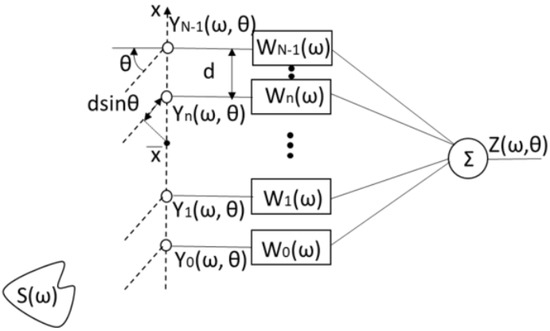
Figure 1.
Beamforming with a linear microphone array configuration.
We analyzed and implemented two different approaches in superdirective data-independent beamforming design described in literature [6,7,8]. To our knowledge, no one in the relevant literature has conducted this important and extremely deep comparison in order to apply further these methods in a real experimental context. Superdirective beamformers are sensitive to the errors in the uniform array characteristics. In the first numerical least-squares method proposed [6,9] a desired beam pattern (BP) profile has to be chosen as input by the user; moreover the frequency and angle independent array characteristics affect the beamformer in a manner close to spatially white noise. Then the white noise gain (Equation (6)) is the way to measure the performances and the robustness of the beamforming design. The method uses a threshold for its value to assure it, as a constraint for the to lie above this value. In the second approach [7,10,11] the BP profile is optimized by the method itself without any user’s choice [12], finding the most directive profile compatibly with the frequency invariance of the real BP. The robustness of the solution is guaranteed taking into account in the synthesis process the errors of the array, using the probability density function (PDF) of the microphones firstly introduced by Doclo and Moonen [8,13], inside the analytic minimization of the cost function. The method uses a cost function written in a closed form, which has an analytic minimum. Both methods deal with data-independent beamformer, which not suffer of problems of signal cancellation in presence of echoes and multipath, as it happens frequently with adaptive methods, so they are very suitable for real applications (phased array for radar, etc.). This paper is organized as follows. Section 2 describes the quantities useful to compare the results and the describes the mathematical background of the two methods implemented, Section 3 reports the conditions and the results of the comparison found, Section 4 comments the results, and Section 5 defines the conclusions and potential new directions of investigation.
2. Materials and Methods
Considering an equi-spaced (d is the constant distance between two microphones) linear array of N omnidirectional point-like sensors each connected to a FIR filter composed of L taps (Figure 1), the BP can be computed as:
where
is the distance of the n-th sensor to the center of the array, L is the FIR’s length, sampling interval of the FIR filter, c the speed of the acoustic waves in the medium, and the weight is a real value representing the l-th tap coefficient of the n-th filter. We can rewrite (Equation (2)) as:
where
Superdirective beamfomers algorithms are extremely sensitive to spatial white noise and to small errors in the array characteristics. These errors are nearly uncorrelated from sensor to sensor and affect the beamformer in a manner similar to spatially white noise. Hence, the is a commonly used measure for the robustness. The is given by:
where is the steering angle ( i.e., broadside geometry and for end-of-fire) (Figure 2).
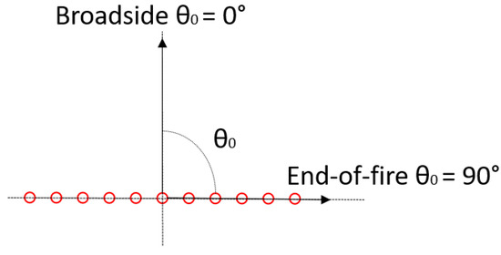
Figure 2.
Broadside end end-of-fire steering directions (broadside orthogonal to the linear array, end-of-fire parallel to the direction of the array).
An assessment of the beamformer performance independent of DOA, is attained through the array gain, which is the improvement in the signal to noise ratio obtained by using the array, when ambient noise is considered as noise. For isotropic noise, the array gain is called and for a linear array is given by:
In the methods of synthesis used, at a certain frequency, the higher is the , the lower is the and the more frequency-invariant is the beampattern generated in the whole bandwidth of interest. Both methods implemented deal with the problem of robustness of super directive beam pattern (BP) against errors in the microphone response due to manufacturing limitations which is the focal and critical point in the real experimental scenario.
2.1. Proposed Methods
2.1.1. Robust Least-Squares Frequency-Invariant Beamformer Design (RLSFIB)
In the first method used [6,14], the data-independent broadband least-squares frequency-invariant beamforming design (LSB), it directly constrains the to lie above a given lower limit by solving a convex optimization problem. The idea behind the design is to optimally approximate a desired response, , by in the least-squares (LS) sense. Typically, a numerical solution is obtained by discretizing the frequency range of the bandwidth into Q frequencies , where and the angular range of the DOA into P angles , where and solving the resulting set of linear equations numerically. Since the number of discretized angles is typically greater than the number of sensors, i.e., , the problem is therefore over-determined. A least-squares frequency-invariant beamformer design (LSFIB) is obtained by choosing the same desired response for all frequencies. This design inherently leads to superdirective beamformers for low frequencies if the wavelengths of the signals involved are larger than twice the sensor spacing and is therefore very sensitive to small random errors encountered in real-world applications. Since the is a measure of the robustness of a beamformer the first algorithm design is then obtained by constraining the above a threshold (Equation (8)). The algorithm imposes in the LS sense solution of the problem a constraint on the that indirectly makes the array robust to errors in microphones. The idea behind the method is to incorporate a constraint into the LSB design by adding the following quadratic constraint. The least-squares solution to this problem, which gives the smallest quadratic error by definition, is given by:
where is the lower bound for the and
where
Moreover, we impose that the desired signal from a given angle (broadside in this case) remains not distorted. This method requires an iterative optimization (sequential quadratic programming , in Matlab) but is able to reach the global minimum since the problem formulation is convex. In this method, the trade-off between frequency-invariant and directivity is given by : the higher is its value, the more the BP pattern will be frequency-invariant and the lower the directivity.
2.1.2. Frequency-Invariant Beam Pattern Design (FIBP)
The second method analyzed [7,10,11,14,15,16] uses a cost function over the probability density function PDF of errors (that must be known), granting in such way a solution that is optimal “on average”. The algorithm proposes a method of FIR synthesis that allows for the design of a robust broadband beamformer with tunable tradeoff between frequency-invariance and directivity, without the need to impose a desired beam pattern [12]. The algorithm uses a cost function minimized with respect to the FIR filter’s coefficient (Equation (10)) and the values of the vector of desired beam pattern (DBP) :
The length of the vector is because the desired beam pattern (DBP) at the steering angle (index ) equals 1 by construction and then is not a part of the vector. The cost function to be minimized is given by next equation:
We impose once again that the desired beam pattern (DBP) from a given angle (in our case broadside) equals 1. Such a cost function (Equation (12)) is made up of two terms: the first term accounts for the adherence between the obtained BP and the DBP in a least-squares sense, and for all the frequencies and directions of interest, and the second one expresses the DBP energy. The relative weight of the two terms is ruled by the K parameter, whose values belong to the interval . Finally, to avoid any distortions of the received signals, the phase of the DBP should be linear, to produce a time delay referred to as . The devised cost function has just one global minimum whose argument can be found in closed form by a computationally inexpensive procedure. The cost function previously described (Equation (12)) is based on the hypothesis that the characteristics of the sensors are perfectly known and not subject to deviations from the nominal values. Consequently, a synthesis based on this cost function, if applied to superdirective arrays, would produce a beamforming characterized by a high sensitivity to errors, especially in the gain and in the phase of the sensors. To overcome this drawback, a robust cost function is introduced. The method includes a subsequent modeling of the amplitude and phase errors of the microphones, of which we assume equal numerical values for the standard deviations. The relationships between mean values and standard deviations (variances) (Equation (13)) are expressed by the same article [7].
The cost function must be minimized with respect to the coefficients of the FIR filters, and to the DBP values, contained in the vector with each discretized DOA except the steering angle. Considering the constraint on the DBP at the steering angle and the definition of directivity, the minimization of the DBP energy (i.e., the second term of the cost function), is equivalent to the maximization of the DBP directivity calculated in an approximate way on a discrete number of angles. In order to get a robust cost function, the formula (Equation (2)) in the previous paragraph can be replaced with:
where
The term is included to take into account the gain and phase characteristics of the n-th sensor, supposed to be frequency invariant. The idea is to optimize the average performance, expressed through the weighted sum of the cost functions calculated for all possible combinations of sensor characteristics, using the probability density functions (PDFs) of the sensor characteristics as weights. For this purpose, a total cost function can be defined in the following equation:
Consider initially the non-robust cost function defined by the expression (Equation (2)), the expression of the BP can be written as:
where is the row vector of size and is the column vector containing the complex exponentials that take into account the delays introduced by the propagation of the plane wave and the delay lines of the filters. Entering the previous relation (Equation (17)) in the expression (Equation (12)) we obtain:
where . We rewrite the cost function in a matrix formulation using the following definitions:
where indicates the index of the direction of steering, the apices the transpose, and the conjugate complex, is the identity matrix of dimensions and is a column vector of size whose elements are all zeros. Introducing the matrix of dimensions defined as follows:
the cost function to be minimized becomes:
whose analytic minimum turns out to be:
The first M elements of represent the optimized FIR’s coefficients while the last elements present the optimized DBPs for all DOAs apart from the steering direction where the DBP is 1 for construction. The matrix (Equation (26)) is positive defined and therefore invertible. The described process can be extended to the minimization of the robust cost function in the following way, replacing the expression of the BP given by the relation (Equation (17)), which contains the model of the errors in amplitude and phase of the microphones within the same cost function (Equation (12)). After some calculations, the matrix expression of the expected cost function is similar to the relation (Equation (27)) with only some modifications of the matrices involved:
where
Finally, the matrix of size M × M is defined as:
The symbol ⊗ indicates the element-wise multiplication and indicates a matrix of size in which all the elements are equal to 1. The solution is given by:
Once the synthesis FIR coefficients’ of the beam pattern have been obtained, the expected beam power pattern (EBPP) can be computed through the expectation operator . The EBPP represents the mean of the actual beam power pattern and is considered the most likely quantity to compared the average performance of different superdirective design methods. The aim is to make a performance average with respect to the randomness of the gain and phase of every array sensor. While the function represents the nominal beam pattern (where all the array sensors have the nominal gain and phase behavior), we can denote by the actual beam pattern, i.e., the beam pattern in which the actual gain and phase (to be intended as realizations of random variables) of each sensor composing the array are duly considered. The EBPP, , is defined as the mean of the actual beam power pattern, as follows: . Working on the expectation operator, the following equation can be reached [7]:
where
Another important parameter to evaluate the synthesis’ performances is given by the generalized directivity [17] (Equation (37)), where k is the wavenumber , and is the steering direction. The n-th element (microphone) is placed at the position and the m-th at the position .
The generalized directivity represents the directivity of the EBPP obtained by using (Equation (7)) and replacing with .
3. Results
Both algorithms and the simulations have been developed and performed under Matlab framework [18,19]. The geometry used for both simulations is broadside () with:
- Aperture of the array 12 cm (length for superdirective beamforming).
- 8 equi-spaced microphones (good compromise between number of microphones and final price of the array).
- Sampling frequency 16 kHz (twice the maximum frequency of the signals involved to respect the Nyquist’s theorem).
- L i.e., FIR’s filter length 128 taps.
- Frequency band of interest (100–8000) Hz (typical bandwidth for audio applications).
- Value of the speed of sound m/s.
- We used a grid of input data dividing the frequency bandwidth of interest Hz in values with a constant step of 50 Hz, and the range of the angles of the direction of arrival in values with a constant step of .
In these conditions, we find d = 1.71 cm then the limit for the spatial aliasing is kHz, outside the band of the interest. To run both simulations we chose and , then for the second algorithm the computational load is related to iterations. For the first RLSFIB algorithm, we chose = −10 dB as the constraint whereas for the second FIBP algorithm we used K = 0.3 as numerical input as a trade-off between frequency-invariant and directivity. With this setting of parameters we get an intermediate synthesis between frequency-variant and frequency-invariant for both algorithms, but this is done to compare, in a fair way, their performances. The PDFs of the microphone gain and phase are assumed to be independent Gaussian functions with a mean equal to 1 and 0, respectively, and with a standard deviation of for both. Once synthesized the two FIR coefficient sets for the two algorithms design, we built up and compared directivities (Figure 3), (Figure 4), directivity and generalized directivity vs standard deviation (Figure 5) and BPs (Figure 6 and Figure 7).
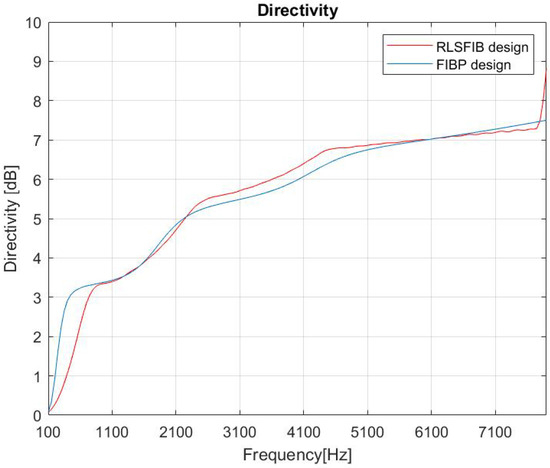
Figure 3.
Directivity comparison: frequency-invariant beam pattern design (FIBP) blue, robust least-squares frequency-invariant beamformer design (RLSFIB) red.
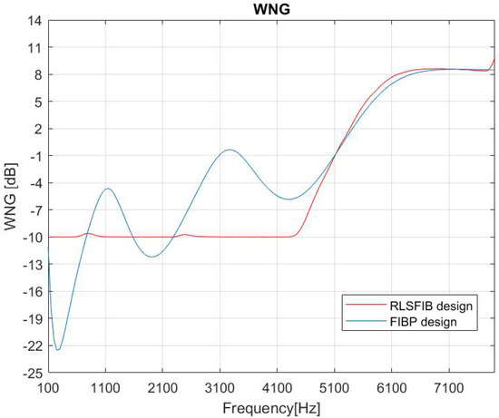
Figure 4.
WNG comparison: FIBP blue, RLSFIB red.
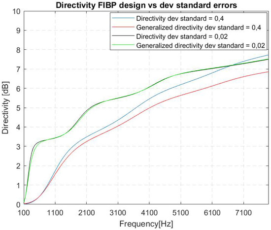
Figure 5.
FIBP design: directivity and generalized directivity vs dev standard comparison.
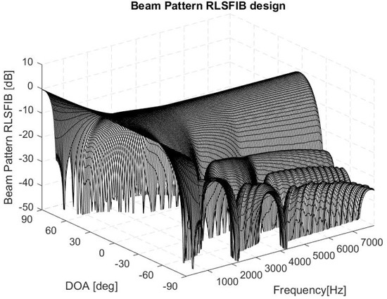
Figure 6.
Beam pattern RLSFIB design.
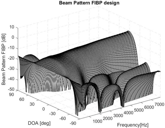
Figure 7.
Beam pattern FIBP design.
3.1. RLSFIB Algorithm
The constrained least-squares problem was shown to be convex and therefore well-established methods for convex optimization, such as the methods and , may be used to solve the constrained problem. The results shown confirm that the RLSFIB design is capable of controlling the robustness of the resulting beamformer, which underlines the flexibility of this design procedure.
3.2. FIBP Algorithm
The robustness of the solution is achieved by taking into account the PDFs of the sensors’ characteristics during the design phase. The EBPP (Figure 8) has been adopted to assess the performance of the beamformers obtained by the proposed synthesis method in addition to the traditional broadband BP graph and the curves of directivity and white noise gain.
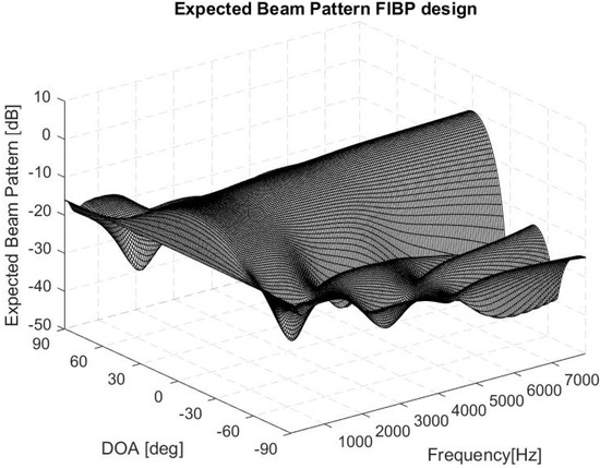
Figure 8.
Expected beam pattern FIBP design.
4. Discussion
In the described simulations, we have chosen a geometry and a set-up of parameters that allows us to make a fair comparison between the performances of the two different design methods analyzed. In particular, we addressed a small linear array for audio capture with different purposes (hearing aids, audio surveillance system, videoconference system, multimedia device, etc.). FIBP presents a more frequency-invariant BP and better performances at lower frequencies. With the parameters’ choice, directivity and are comparable for the two methods at the higher frequencies, but at lower frequencies has an oscillating behavior for FIBP method, avoided by definition for the RLSFIB design. The oscillating behavior of the in the FIBP method is due to the fact that, in general, and are mutually reciprocals. In fact, when the derivative of directivity in the FIBP method is high (Figure 3, blue line), the is low and vice versa. We can see that the first derivative of the directivity of the FIBP method is changing a lot in the range Hz: that is why the is oscillating (Figure 4, blue line). The change of the first derivative is less pronounced for the directivity of the RLSFIB method (Figure 3, red line). Moreover, the threshold in the forces this parameter to have a flatter and more stable curve (Figure 4, red line). The directivity at low frequencies provided by the RLSFIB method, lower than that provided by the FIBP method, justifies why the shape of the beam pattern (Figure 6) has a main lobe wider that of the FIBP method (Figure 7). The great advantage of the FIBP is the possibility to change the deviation standard of the distribution of the errors to highlight its impact: increasing the standard deviation, the difference between directivity and generalized directivity increases as well (Figure 5). This fact for FIBP design is very interesting because the difference between the generalized directivity and the nominal one provides useful insight on the expected impact that a given level of microphone mismatches induces on the system performance. This analysis allows us to choose the microphone accuracy, which is necessary to limit the (mean) performance decay at the level the user requires. A potential future work is to compare the performances of the two approaches for more frequency-variant rather then frequency-invariant synthesis, playing respectively with and K, comparing once again both performances of the algorithm of FIR’s synthesis, using respectively, a lower and a higher K with respect the current values.
5. Conclusions
In this paper we presented and compared the metrics of the synthesis of two different methods of simulation, following two different philosophies, to get the synthesis of FIR’s coefficient filters for an efficient and robust superdirective beamformer to target audio applications in a real experimental scenario using a compact linear array of microphones. The main drawback of the two methods presented is the limitation on the choice of the cost function forced by the convexity conditions. In particular, there is no way to differentiate between main lobe and side lobe region, or to impose a worst-case design by minimizing the maximum of the side lobes. Moreover cost functions are quadratic so that low energy regions of BP are not very weighted in the cost function. Working with different representations (logarithmic) of BP could allow for a better shaping of low energy regions. For all these reasons, for further development of a new and better method of synthesis, the cost function should be modified to lose the convexity property. Then, to face the related problem of local minima, it would be necessary to take into account heuristics algorithms such as genetic algorithms. The simulations presented in this paper allow us to point out, for the two compared design methods, the tradeoff between performance (directivity), invariance, robustness (), and sensor accuracy. They represent a starting base for further investigations the reader can perform, providing an insight on the parameters to modify in order to achieve the desired performance.
Author Contributions
A.T.: Conceptualization, Supervision, Knowledge of the Methods; D.G.: Investigation, Formal analysis, Methodology, Conduct of Research, Software Implementation, Data Curation, Drafting of the Article. All authors have read and agreed to the published version of the manuscript.
Funding
This research received no external funding.
Conflicts of Interest
The authors declare no conflict of interest.
References
- Veen, B.D.V.; Buckley, K.M. Beamforming: A versatile approach to spatial filtering. IEEE Assp Mag. 1998, 5, 4–24. [Google Scholar] [CrossRef]
- Ward, D.B.; Kennedy, R.A.; Williamson, R.C. FIR filter design for frequency invariant beamformers. IEEE Signal Process. Lett. 1996, 3, 69–71. [Google Scholar] [CrossRef]
- Ward, D.B.; Kennedy, R.A.; Williamson, R.C.; Brandstein, M. Microphone Arrays Signal Processing Techniques and Applications (Digital Signal Processing); Springer: Berlin/Heidelberg, Germany, 2001. [Google Scholar]
- Trees, H.L.V. Optimum Array Processing: Part IV of Detection, Estimation, and Modulation Theory; John Wiley & Sons, Inc.: Hoboken, NJ, USA, 2002. [Google Scholar]
- Ward, D.B.; Kennedy, R.; Williamson, R. Theory and design of broadband sensor arrays with frequency invariant far-field beam patterns. J. Acoust. Soc. Am. 1999, 97, 1023–1034. [Google Scholar] [CrossRef]
- Mabande, E.; Schad, A.; Kellermann, W. Design of robust superdirective beamformers as a convex optimization problem. In Proceedings of the 2009 IEEE International Conference on Acoustics, Speech and Signal Processing, Taipei, Taiwan, 19–24 April 2009; pp. 77–80. [Google Scholar] [CrossRef]
- Crocco, M.; Trucco, A. Design of robust superdirective arrays with a tunable tradeoff between directivity and frequency-invariance. IEEE Trans. Signal Process. 2011, 59, 2169–2181. [Google Scholar] [CrossRef]
- Doclo, S.; Moonen, M. Superdirective Beamforming Robust Against Microphone Mismatch. IEEE Trans. Audio Speech Lang. Process. 2007, 15, 617–631. [Google Scholar] [CrossRef]
- Doclo, S. Multi-Microphone Noise Reduction and Dereverberation Techniques for Speech Applications. Ph.D. Thesis. Available online: ftp://ftp.esat.kuleuven.ac.be/stadius/doclo/phd/ (accessed on 23 May 2003).
- Crocco, M.; Trucco, A. The synthesis of robust broadband beamformers for equallyspaced array. J. Acoust. Soc. Am. 2010, 128, 691–701. [Google Scholar] [CrossRef] [PubMed]
- Crocco, M.; Trucco, A. Stochastic and Analytic Optimization of Sparse Aperiodic Arrays and Broadband Beamformers With Robust Superdirective Patterns. IEEE Trans. Audio Speech Lang. Process. 2012, 20, 2433–2447. [Google Scholar] [CrossRef]
- Trucco, A.; Crocco, M.; Traverso, F. Avoiding the imposition of a desired beam pattern in superdirective frequency-invariant beamformers. In Proceedings of the 26th Annual Review of Progress in Applied Computational Electromagnetics, Tampere, Finland, 26–29 April 2010; pp. 952–957. [Google Scholar]
- Doclo, S.; Moonen, M. Design of Broadband Beamformers Robust Against Gain and Phase Errors in the Microphone Array Characteristics. IEEE Trans. Signal Process. 2003, 51, 2511–2526. [Google Scholar] [CrossRef]
- Mabande, E. Robust Time-Invariant Broadband Beamforming as a Convex Optimization Problem. Ph.D. Thesis. Available online: https://opus4.kobv.de/opus4-fau/frontdoor/index/index/year/2015/docId/6138/ (accessed on 10 April 2015).
- Trucco, A.; Traverso, F.; Crocco, M. Robust Superdirective End-Fire Arrays. In Proceedings of the OCEANS’13 IEEE Bergen Conference, Bergen, Norway, 10–14 June 2013; pp. 1–6. [Google Scholar] [CrossRef]
- Traverso, F.; Crocco, M.; Trucco, A. Design of Frequency-Invariant Robust Beam Patterns by the Oversteering of End-Fire Arrays. Signal Process. 2014, 99, 129–135. [Google Scholar] [CrossRef]
- Trucco, A.; Crocco, M. Design of an Optimum Superdirective Beamformer Through Generalized Directivity Maximization. IEEE Trans. Signal Process. 2014, 62, 12. [Google Scholar] [CrossRef]
- Trucco, A.; Traverso, F.; Crocco, M. Broadband performance of superdirective delay-and-sum beamformers steered to end-fire. J. Acoust. Soc. Am. 2014, 135, EL331–EL337. [Google Scholar] [CrossRef] [PubMed]
- Crocco, M.; Trucco, A. A Synthesis Method for Robust Frequency-Invariant Very Large Bandwidth Beamforming. In Proceedings of the 18th European Signal Processing Conference (EUSIPCO 2010), Aalborg, Denmark, 23–27 August 2010; pp. 2096–2100. [Google Scholar]
© 2020 by the authors. Licensee MDPI, Basel, Switzerland. This article is an open access article distributed under the terms and conditions of the Creative Commons Attribution (CC BY) license (http://creativecommons.org/licenses/by/4.0/).