ACAT1 Benchmark of RANS-Informed Analytical Methods for Fan Broadband Noise Prediction—Part I—Influence of the RANS Simulation

 , ,
, , 
Abstract
1. Introduction
- the RANS input,
- the preparation of the RANS input (i.e the extraction of flow and geometry, the reconstruction of wake flow and turbulence, the determination of integral turbulent length scales, etc.),
- and the applied acoustic model.
2. Methods
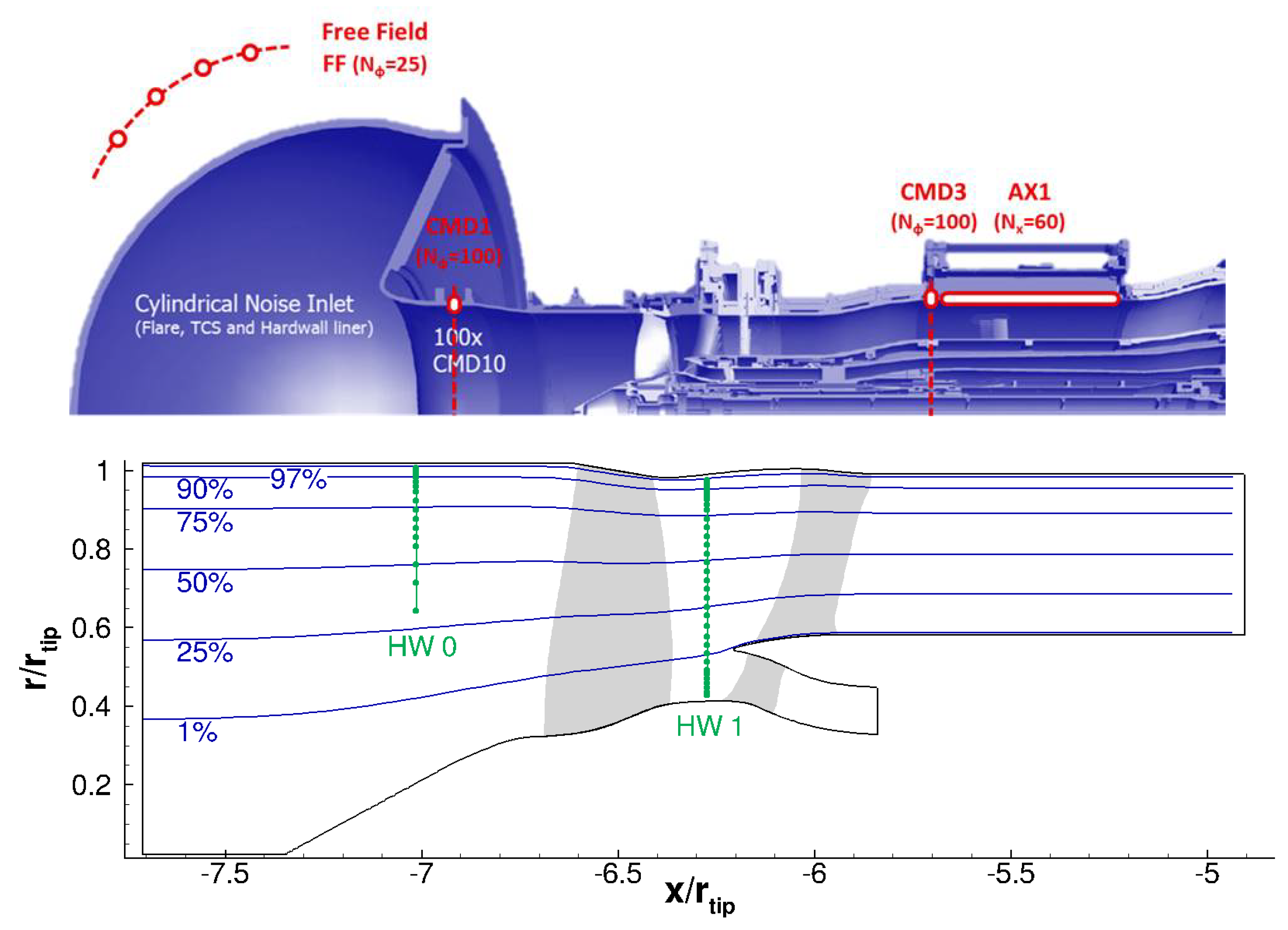
2.1. Experimental Setup and Used Measurement Data
2.2. RANS-Informed Analytical Methods
2.2.1. RANS Simulations and Turbulence Modeling
Linear Eddy Viscosity Turbulence Models
Non-Linear Eddy Viscosity Turbulence Models
Extensions of Eddy Viscosity Turbulence Models
Differential Reynolds Stress Turbulence Models
2.2.2. Preparation of the RANS Input
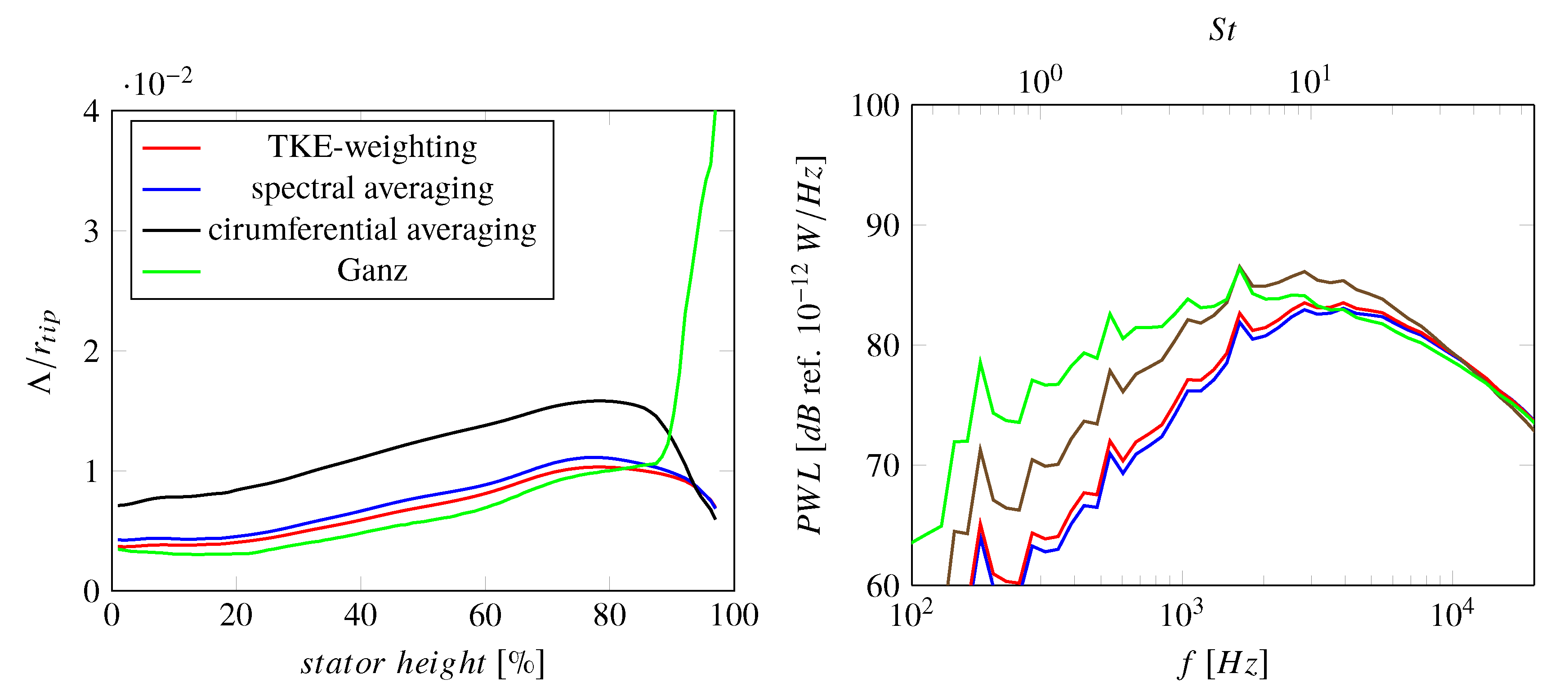
- a length scale determined by fitting the circumferential average of turbulence velocity frequency spectra with a target spectrum [38],
- a Pope-based length scale computed from circumferentially averaged turbulence characteristics ,
- and a Ganz-based, empirically motivated length scale (where A represents the wake area and d the wake velocity deficit) [39].
2.2.3. Analytical Acoustic Model
2.2.4. Post-Processing of Acoustic Results
2.3. Overview of Used RANS Simulations
2.3.1. Solvers and Turbulence Models
2.3.2. Operating Conditions
2.3.3. Geometry and Meshing
3. Results and Discussion
3.1. Influence of the Menter SST k- Turbulence Model
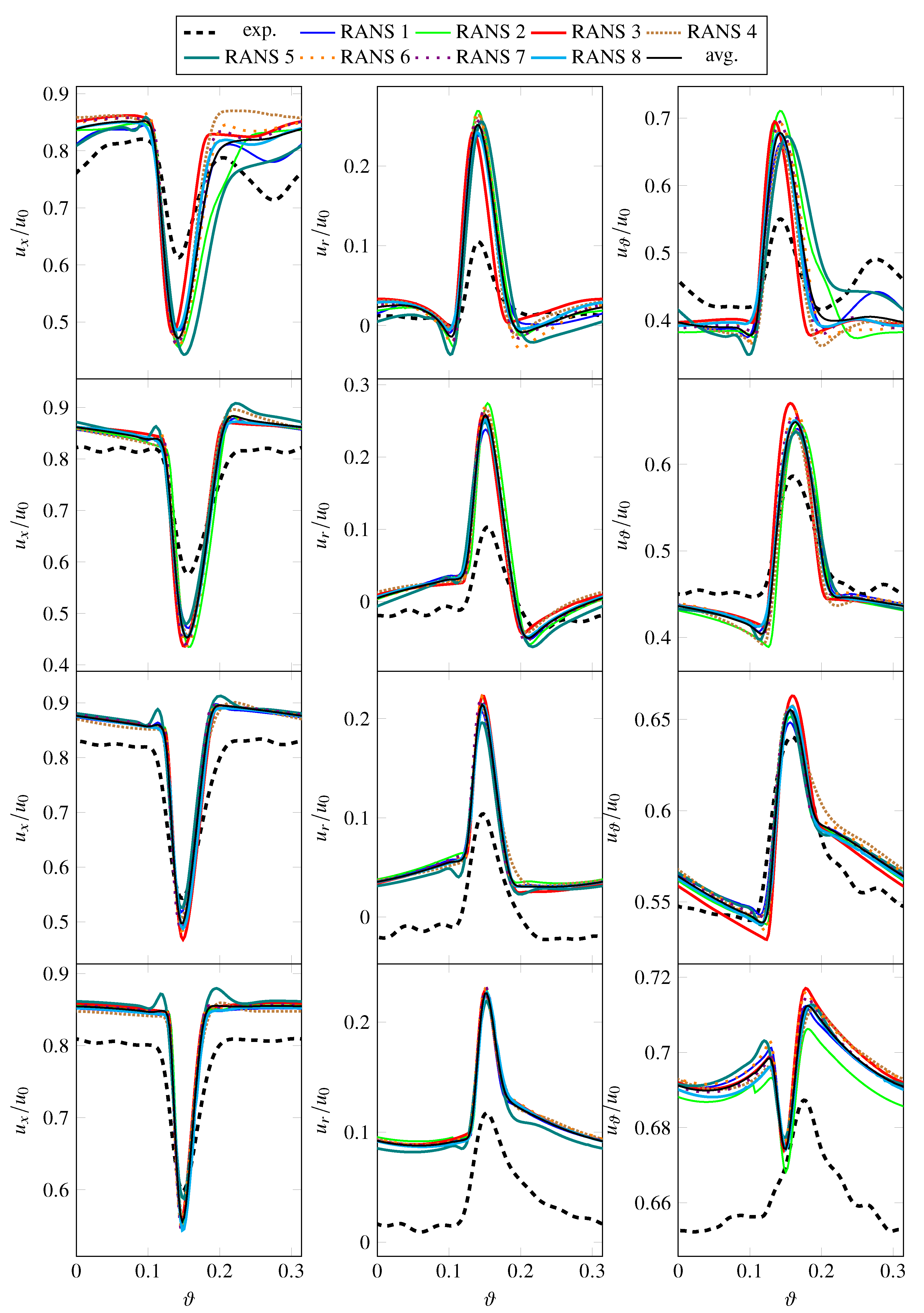
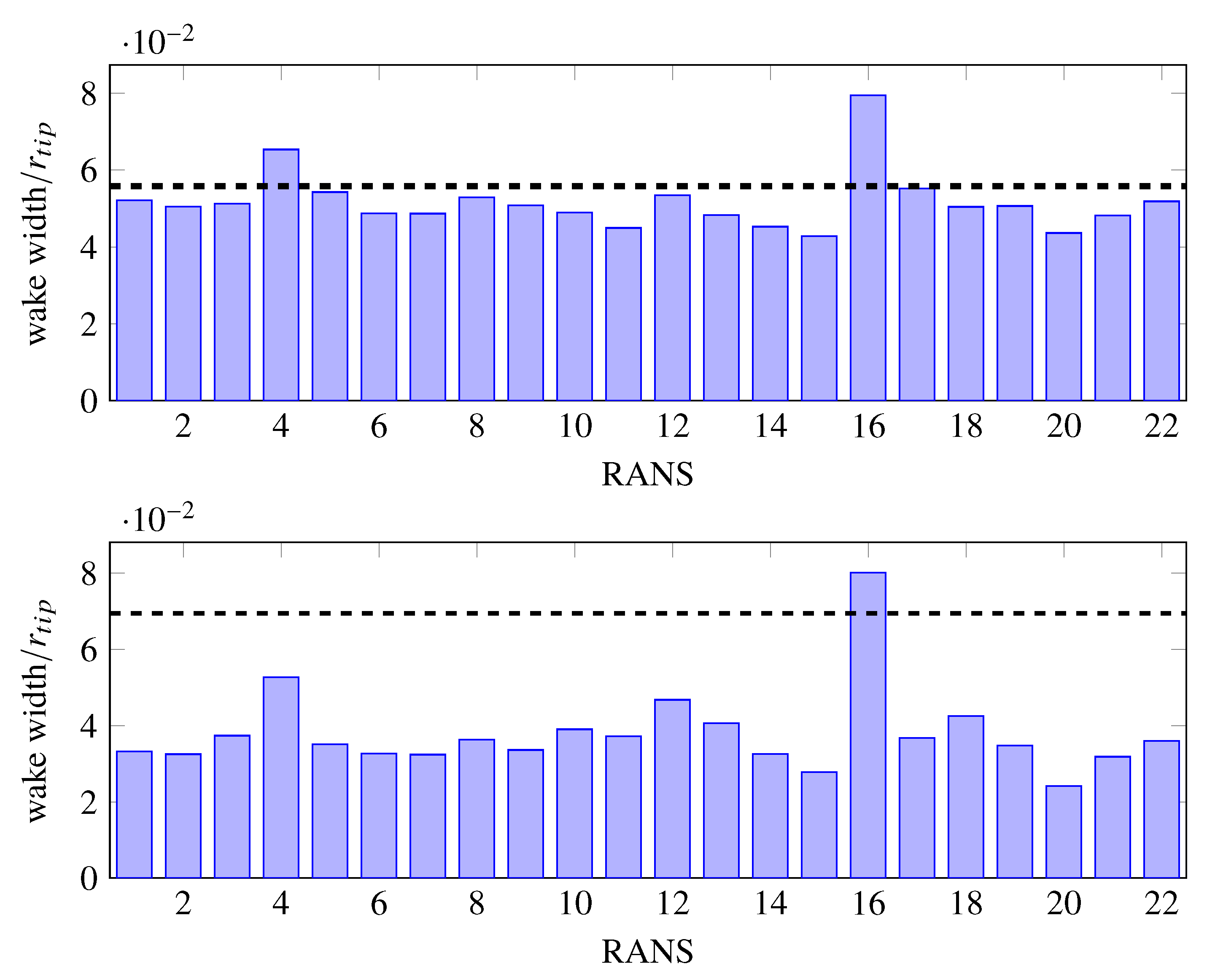
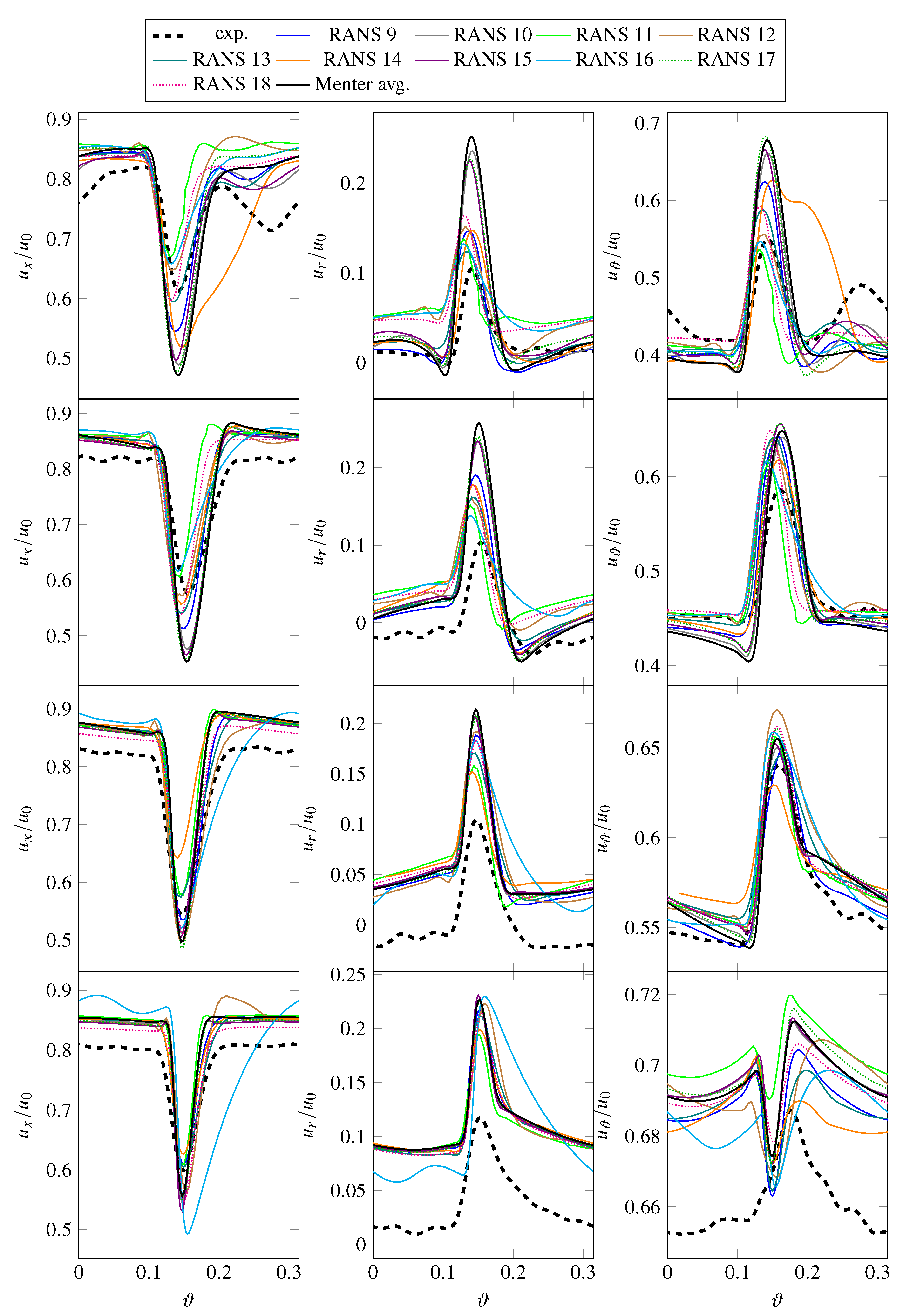
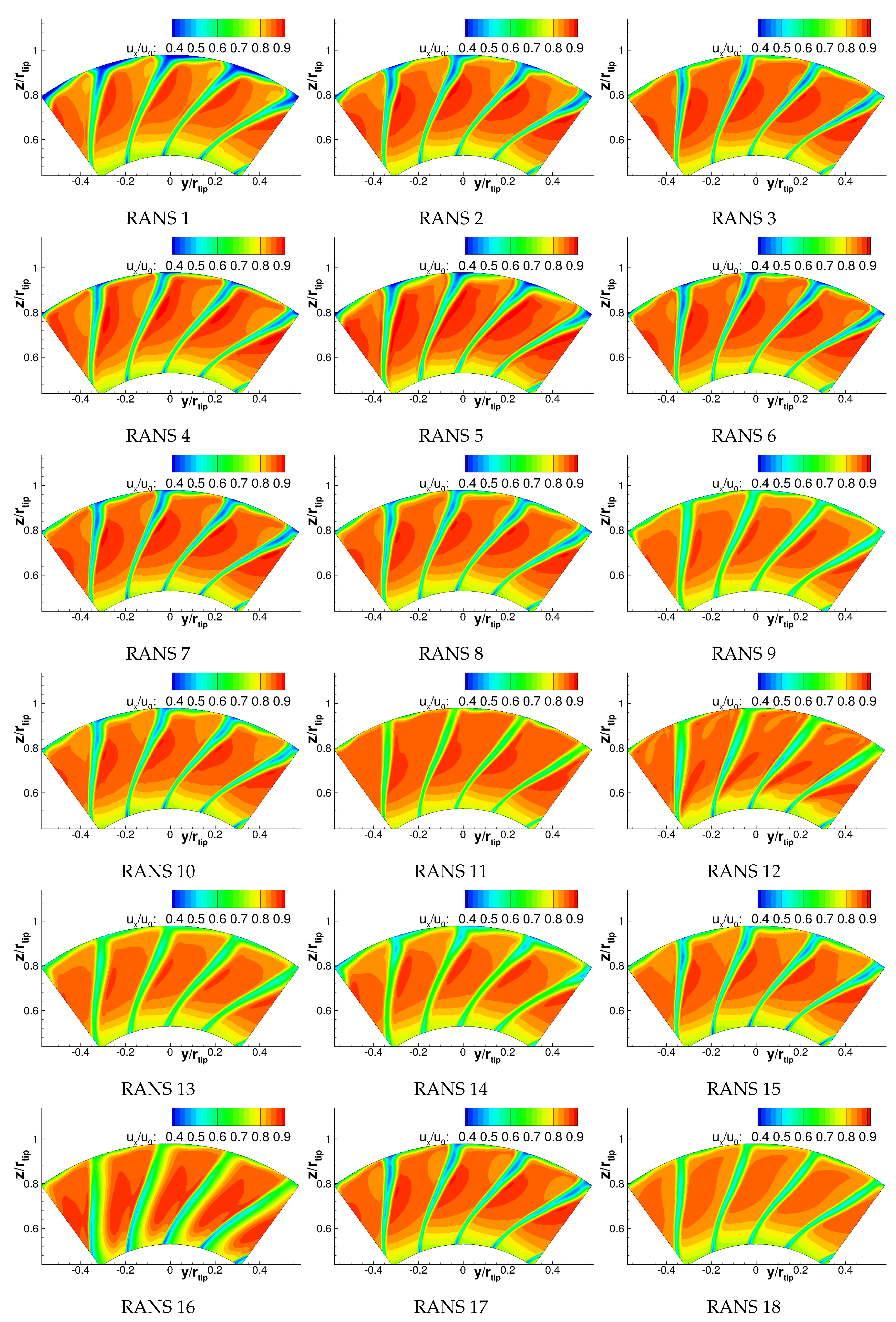
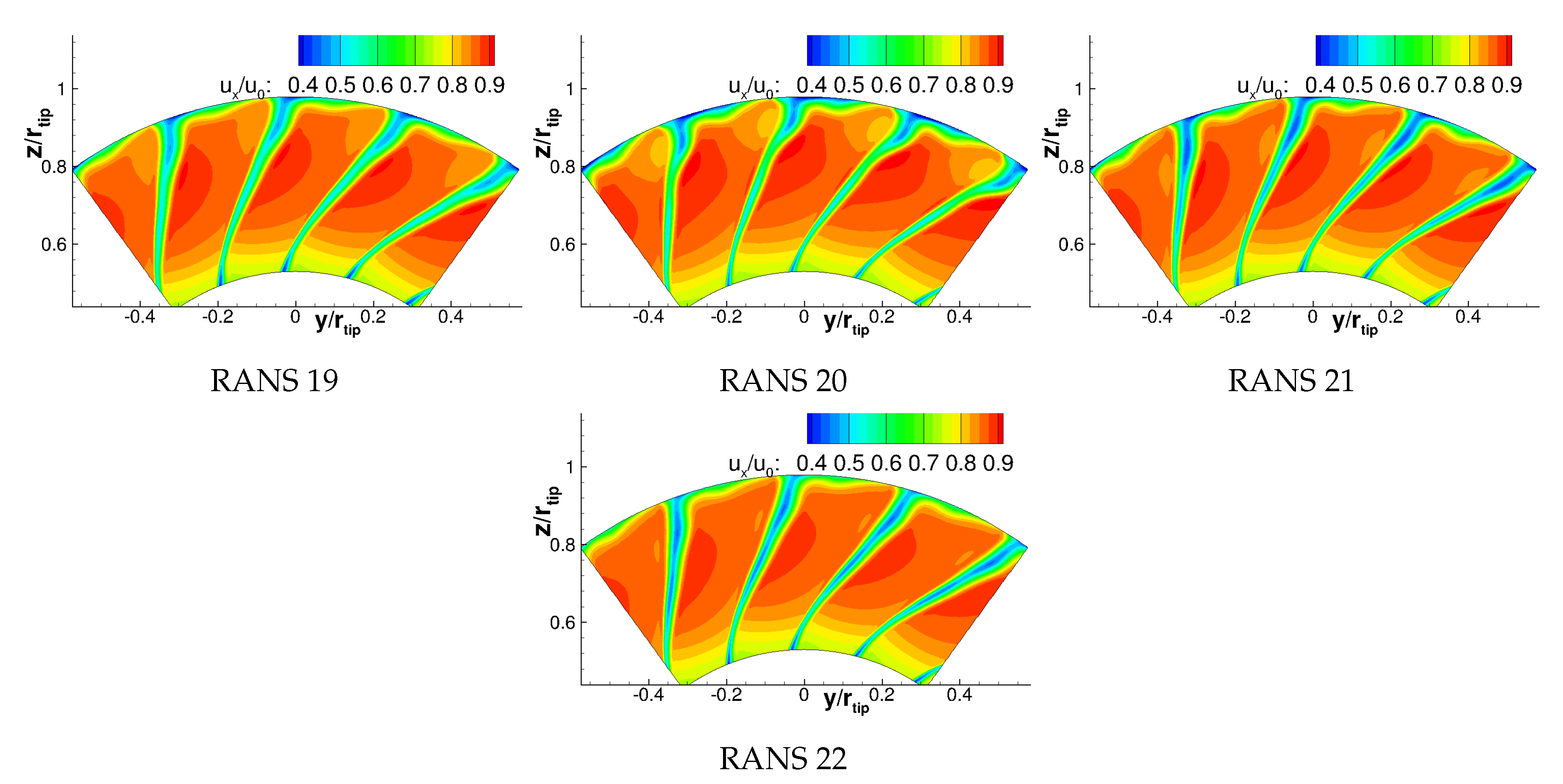
- The wake width is a bit larger in the experiment than in the simulations, especially at lower radial positions. One explanation for this phenomenon is that the hot-wire probes cover a measuring volume of 1 × 2 × 2 mm [10], which defines the spatial resolution. Therefore, the slope of the shear layers are “smeared” and wakes appear to be wider as they are in reality.
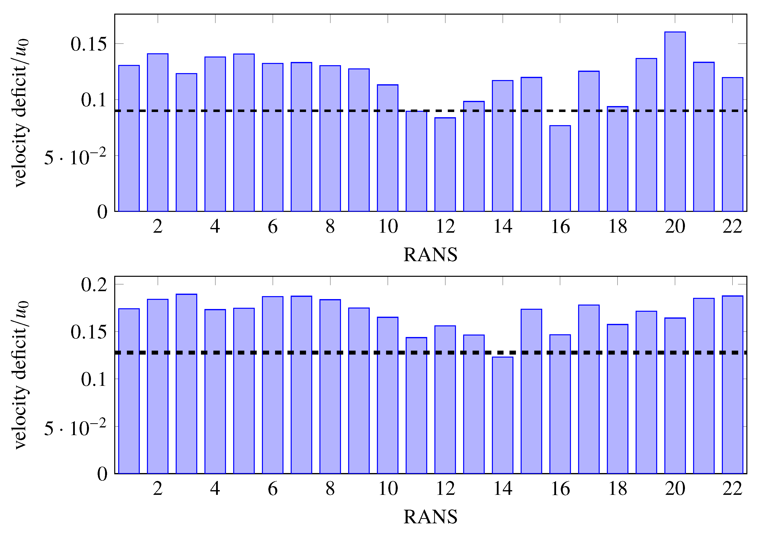
- The wake velocity deficit is smaller in the experiment than in the simulations. Part of the reason for this offset is likely physical in nature. Particularly near the tip region, the wake velocity deficit in the experiment is less pronounced due to a less severe (or absent) leading edge flow detachment compared to the simulations, where it causes deeper and thicker wakes. Another part of the explanation may be due to the hot-wire measurement. The previously mentioned control volume can also cause flatter peaks. In addition, the hot-wire probes were calibrated at one radial position upstream of the rotor blades. Since the in-duct calibration was performed for circumferentially uniform flow, it can be expected that the calibration may not work as well within the wake as outside of it as the temperature increases inside the wakes.
- There are some offsets in mean velocities outside of the wakes. Smaller offsets are indeed expected as the hot-wire probes are less accurate in measuring mean velocities as opposed to fluctuating velocities. Offsets in the radial velocity can occur if the yaw angle of an X-wire probe intended to measure axial and radial velocities is not well aligned with the mean flow. The circumferential velocity component then creates an additional cooling effect, which will be interpreted as partly axial and radial velocity. Since the radial component is significantly smaller than the axial and circumferential components, it is most susceptible to such an effect. The trends of the circumferential velocities at 25% of the stator height diverge, which may be due to the fact that the differences are quite small and likely difficult to capture.
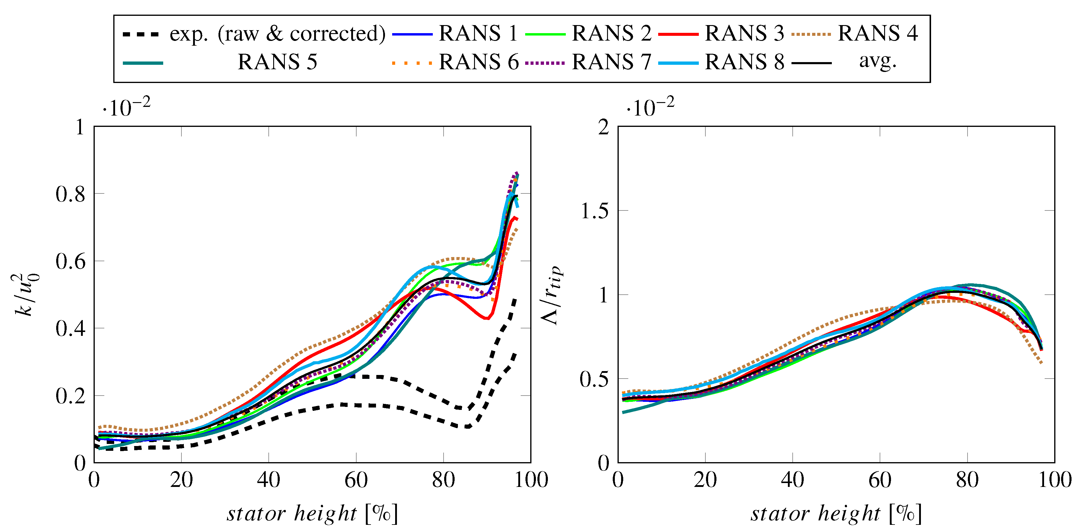
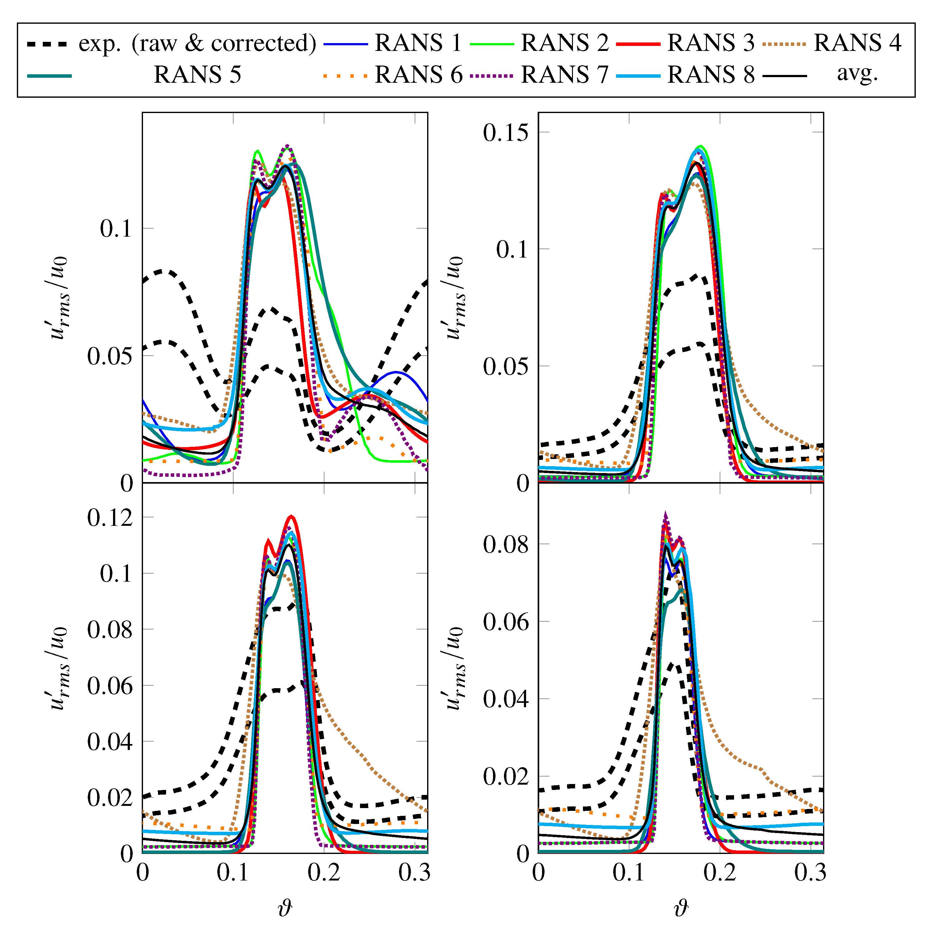
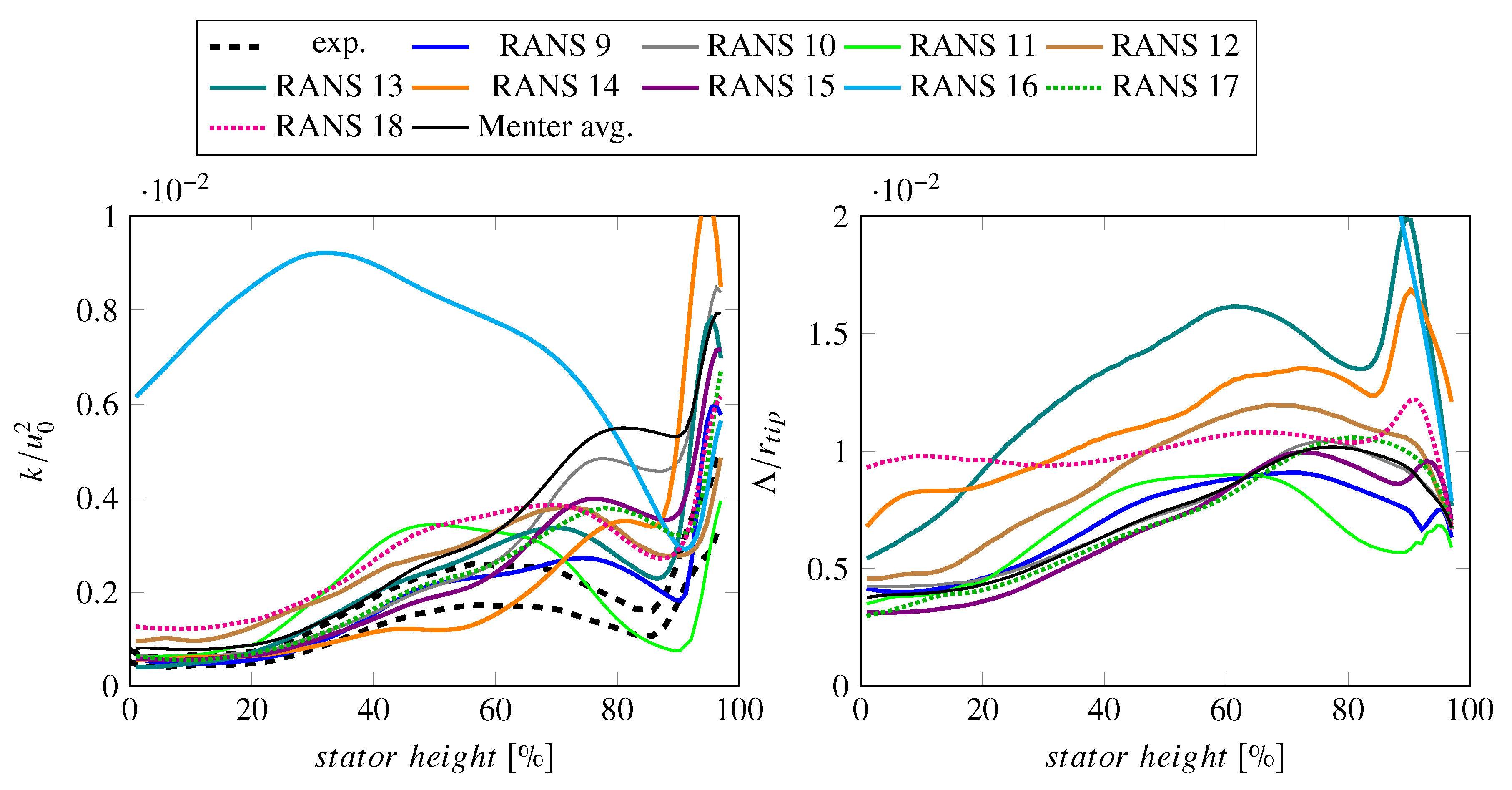
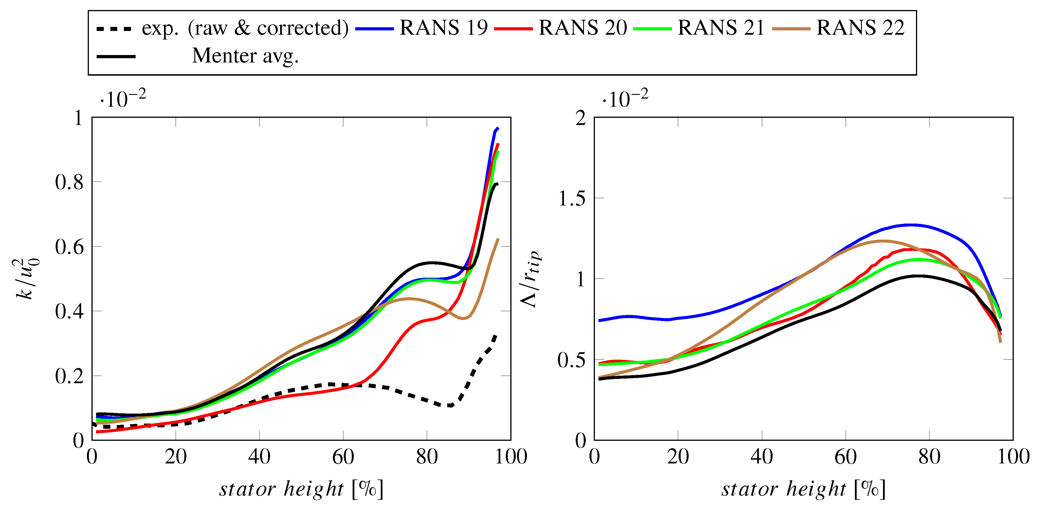
- Turbulent RMS velocities are overpredicted in the RANS simulations, particularly at 75% and 90% stator heights. It should be noted that there is some uncertainty regarding the measured fluctuating velocities. The lower, experimental line in Figure 9 are values directly determined from the measured data, while the upper line includes a factor of 1.5. The thickness of the hot-wires reduces the frequency resolution of the measured data. In this case, the cut-off frequency (or resolution limit) was a posteriori estimated to be around 7–8 kHz. Polacsek et al. [51] have introduced a correction factor of 1.5, which was determined by extrapolating the measured levels beyond the cut-off limit relative to the results of a scale-resolving simulation. For this reason, the raw as well as the corrected experimental values are shown in subsequent figures featuring either turbulent kinetic energies or RMS velocities. It should again be highlighted that the hot-wire calibration may be less suited for determining values within the wake than outside of the wake. Part of the observed offset in RMS velocities may, however, be physical as the higher turbulence levels in the RANS simulations are probably caused by a larger separation at the rotor leading edge than in the experiment. At 90% of the stator height, the measured values also capture the structure of the tip vortex resulting in two peaks.
3.2. Influence of Linear Eddy Viscosity Turbulence Models
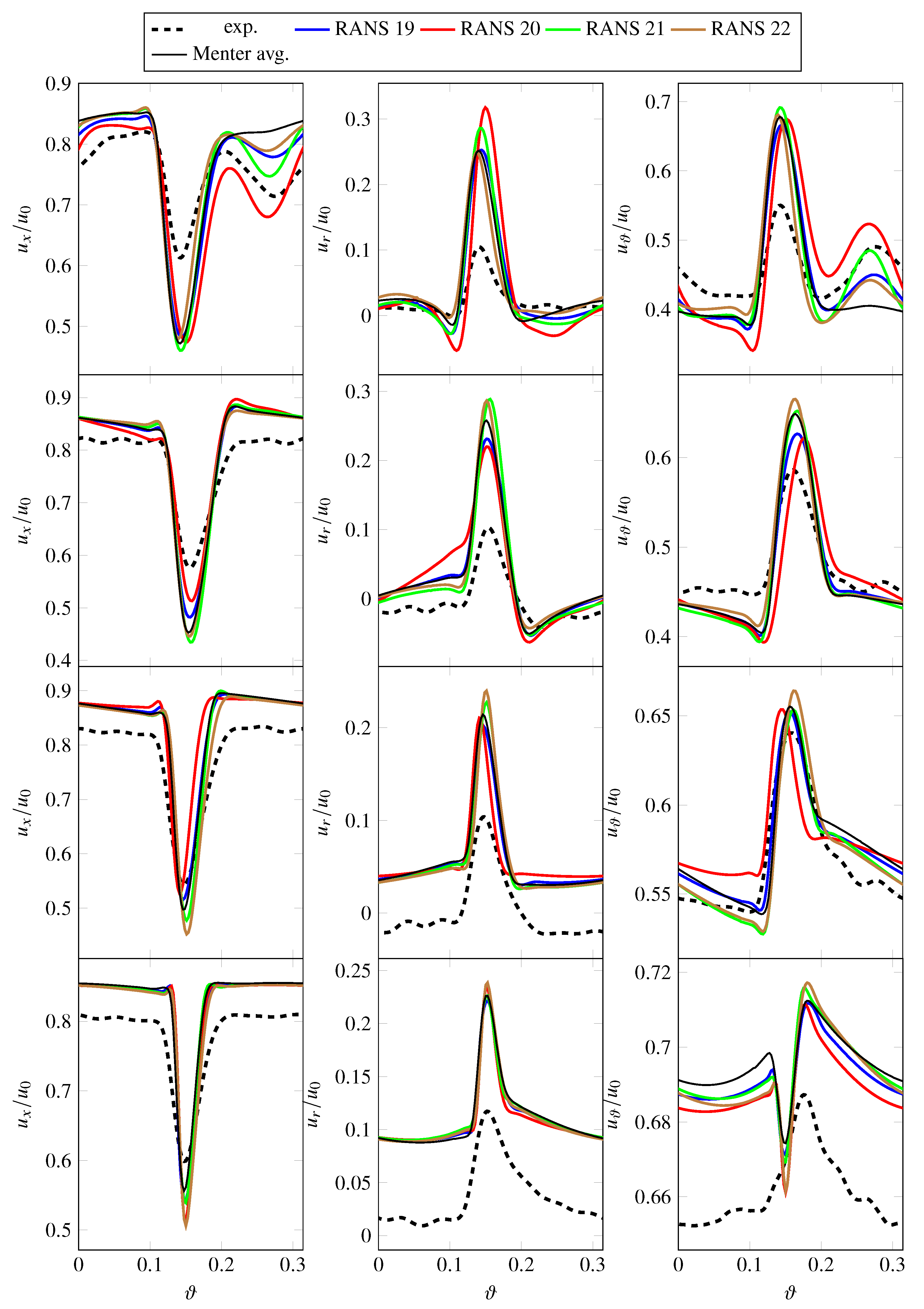
3.3. Influence of More Advanced Turbulence Models
4. Conclusions
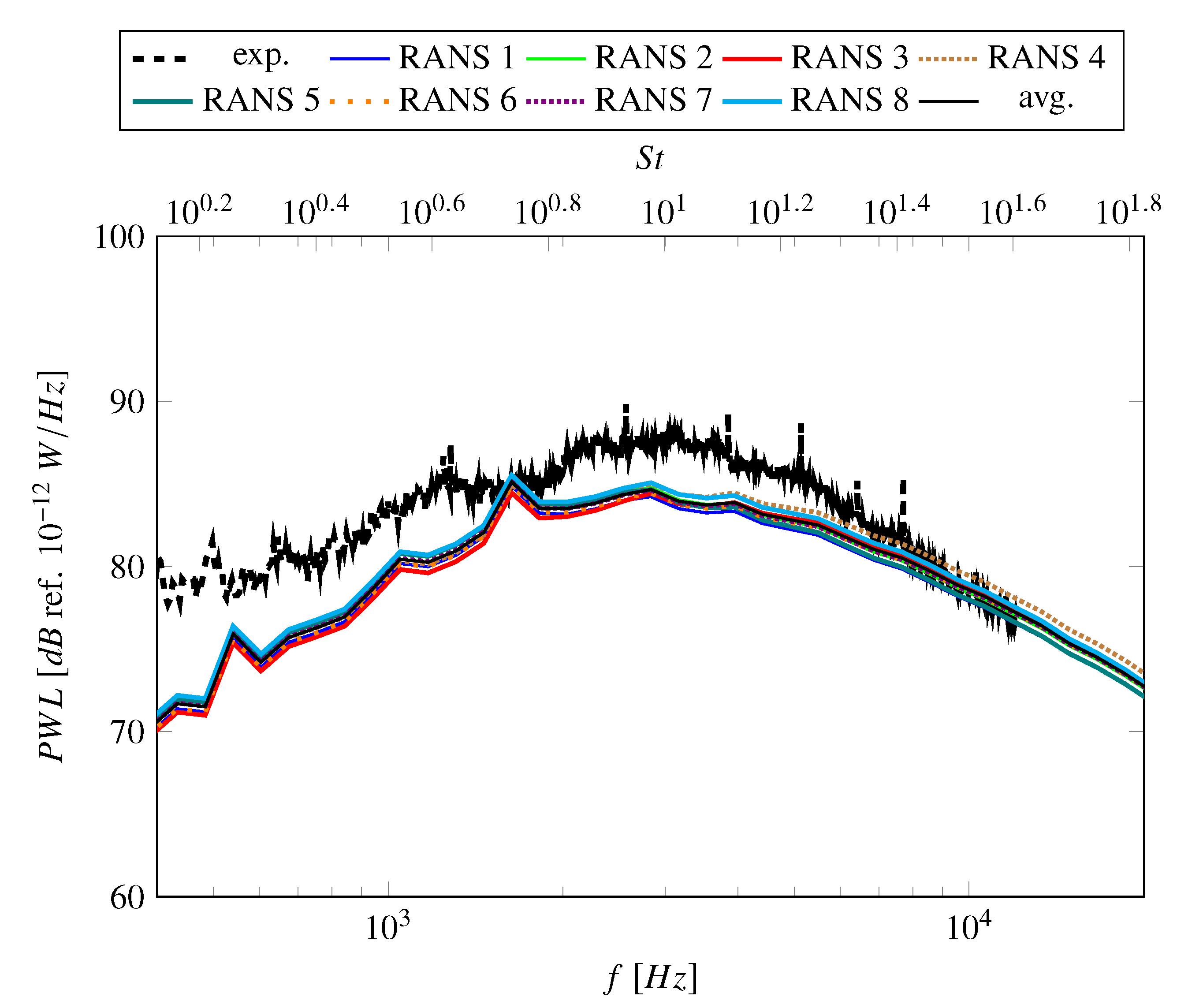
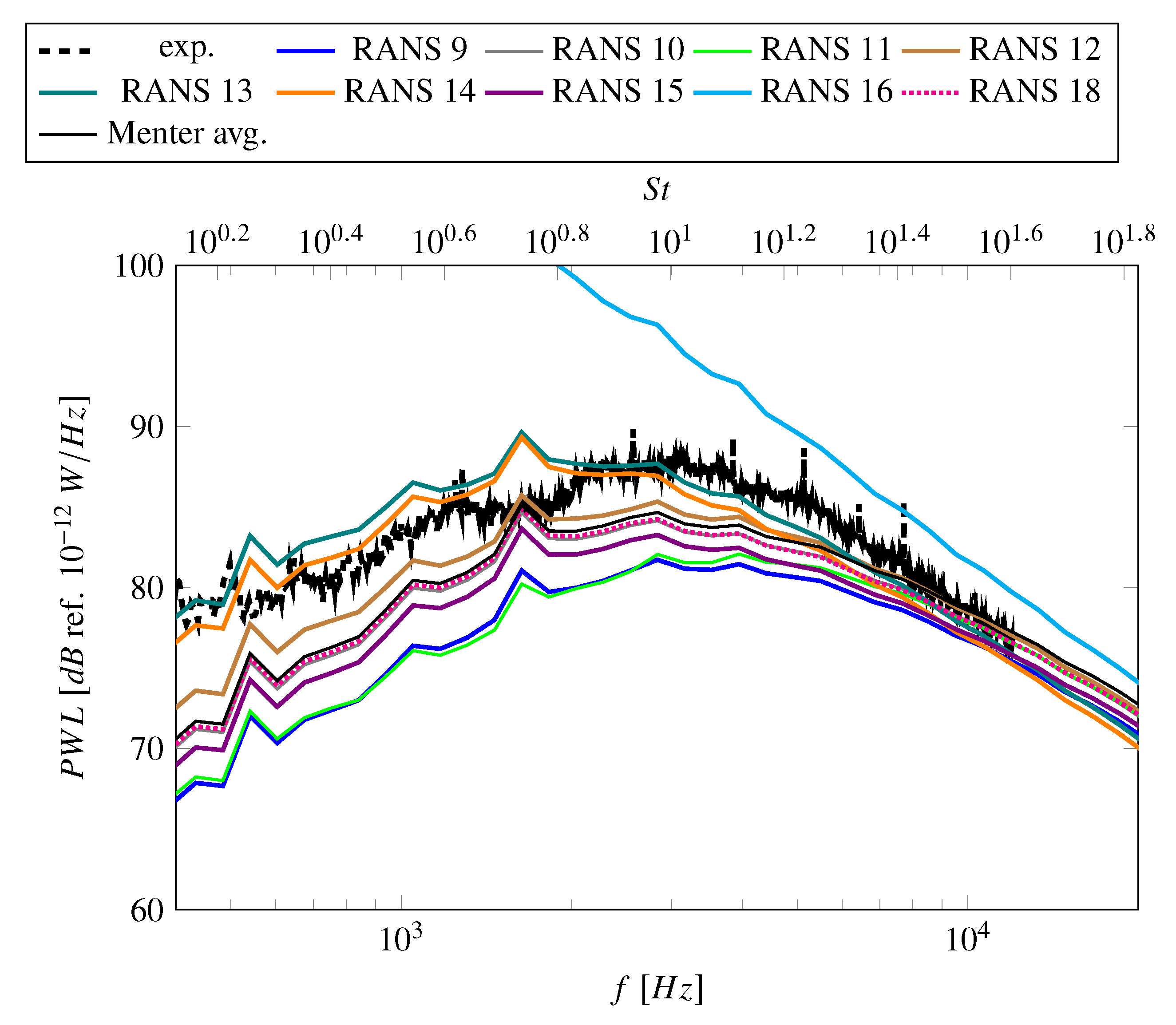
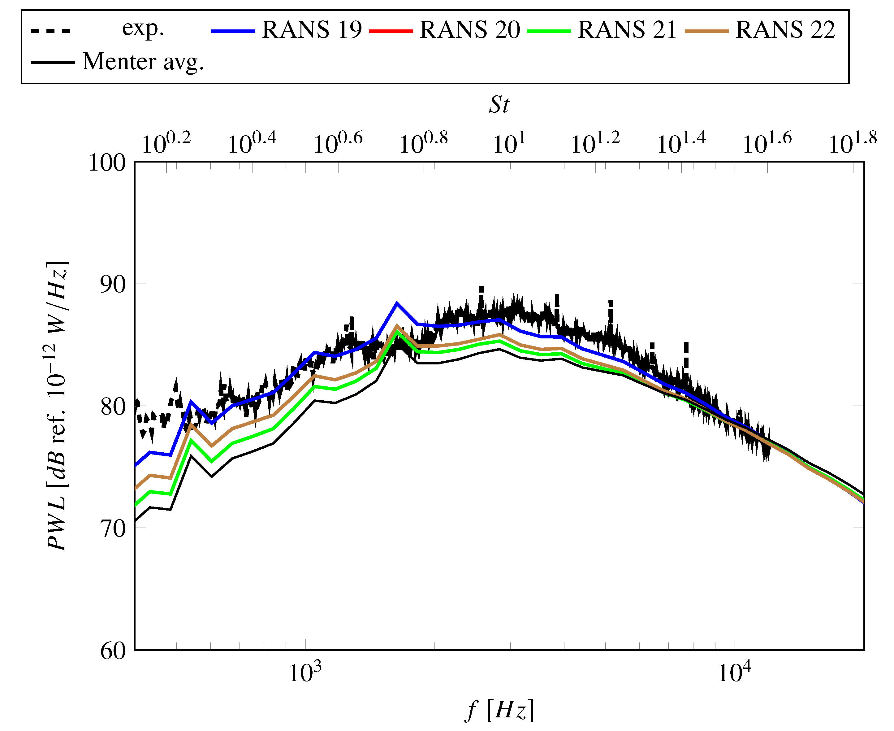
- The Menter SST k- turbulence model and related turbulence models (like the Hellsten EARSM k- or the SSG/LRR-) tend to exaggerate flow separations leading to increased turbulence production. This leads to an increase of sound power levels leading to a better agreement with measured sound power levels but increases the offset between simulated and measured velocities. The Hellsten EARSM k- also causes an increase in turbulent length scale, which is advantageous in terms of sound power levels.
- The Smith k-l turbulence model predicts a weaker flow separation resulting in a better agreement with hot-wire measurements. Due to an increase in predicted TLS, the predicted sound power levels are similar to sound power levels predicted using a Menter SST k- turbulence model. For the investigated case, the Smith k-l turbulence model may be the best compromise between matching hot-wire and acoustic measurements.
- The use of differential Reynolds stress models did not improve results in terms of flow and turbulence characteristics and in terms of fan broadband noise. Unless the objective is to study anisotopic turbulence in more detail, simpler models should be used as they are more robust and require less computational resources.
- Stagnation fixes need to be used for turbulence model featuring an equilibrium formulations. For other turbulence models, stagnation fixes further reduce turbulence production. The reduction of turbulence production leads to a further reduction of predicted fan broadband noise leading to a worse agreement with measurements. The use of stagnation fixes does not significantly improve the agreement with hot-wire data. If the use of stagnation point is necessary, a simple limiter or a local modification of transport equations limited to areas of non-equilibrium flows are preferable.
- Rotational fixes can be used to achieve a better agreement between hot-wire measurements and simulated velocities.
- The use of transition model does not improve fan broadband noise predictions or the agreement with hot-wire measurements.
Author Contributions
Funding
Acknowledgments
Conflicts of Interest
Nomenclature
| A | wake area, m |
| Reynolds number-dependent constant | |
| turbulence model-dependent constant | |
| d | wake velocity deficit, m/s |
| f | frequency, Hz |
| k | turbulent kinetic energy, m/s |
| wake width, m | |
| l | pseudo turbulent length scale (Smith), m |
| sound power level, dB ref. W/Hz | |
| averaged tip rotor radius, 0.428 m | |
| transition Reynolds number based on the momentum thickness | |
| mean strain rate tensor, 1/s | |
| Strouhal number | |
| u | velocity, m/s |
| total mean velocity at the HW 1 position, 128 m/s | |
| intermittency | |
| turbulent dissipation rate, m/s | |
| angle, rad | |
| integral turbulent length scale, m | |
| eddy viscosity, m/s | |
| density, kg/m | |
| Reynolds stress tensor, kg/(s m) | |
| turbulence velocity frequency spectrum (relative to direction i), m/s | |
| vorticity tensor, 1/s | |
| specific turbulent dissipation rate, 1/s | |
| specific homogeneous dissipation rate, 1/s |
Abbreviations
| ACAT1 | AneCom AeroTest Rotor 1 |
| CFD | Computational Fluid Dynamics |
| DNS | Direct Numerical Simulation |
| DRSM | Differential Reynolds Stress Model |
| EARSM | Explicit Algebraic Reynolds Stress Model |
| HW | Hot-Wire |
| ISA | International Standard Atmosphere |
| JH | Jakirlic-Hanjalic |
| LE | Leading Edge |
| LRR | Launder-Reece-Rodi |
| NASA | National Aeronautics and Space Administration |
| PWL | Sound Power Level |
| RANS | Reynolds-Averaged Navier-Stokes |
| RMS | Root Mean Square |
| RSI | Rotor-Stator-Interaction |
| TE | Trailing Edge |
| TKE | Turbulent Kinetic Energy |
| TLS | Turbulent Length Scale |
| SDT | Source Diagnostic Test |
| SSG | Speziale-Sarkar-Gatski |
| SST | Shear-Stress-Transport |
| UFFA | Universal Fan Facility for Acoustics |
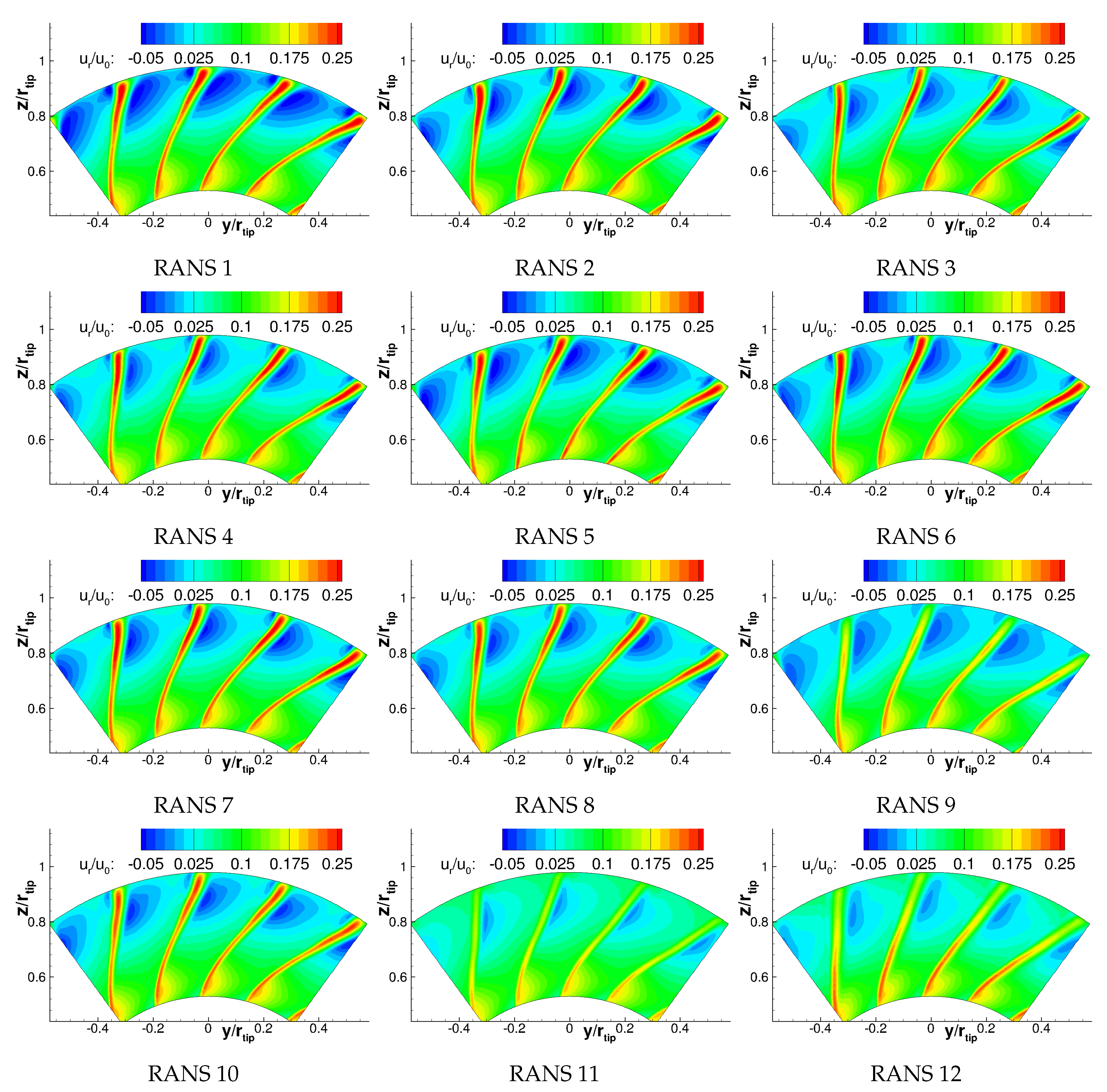
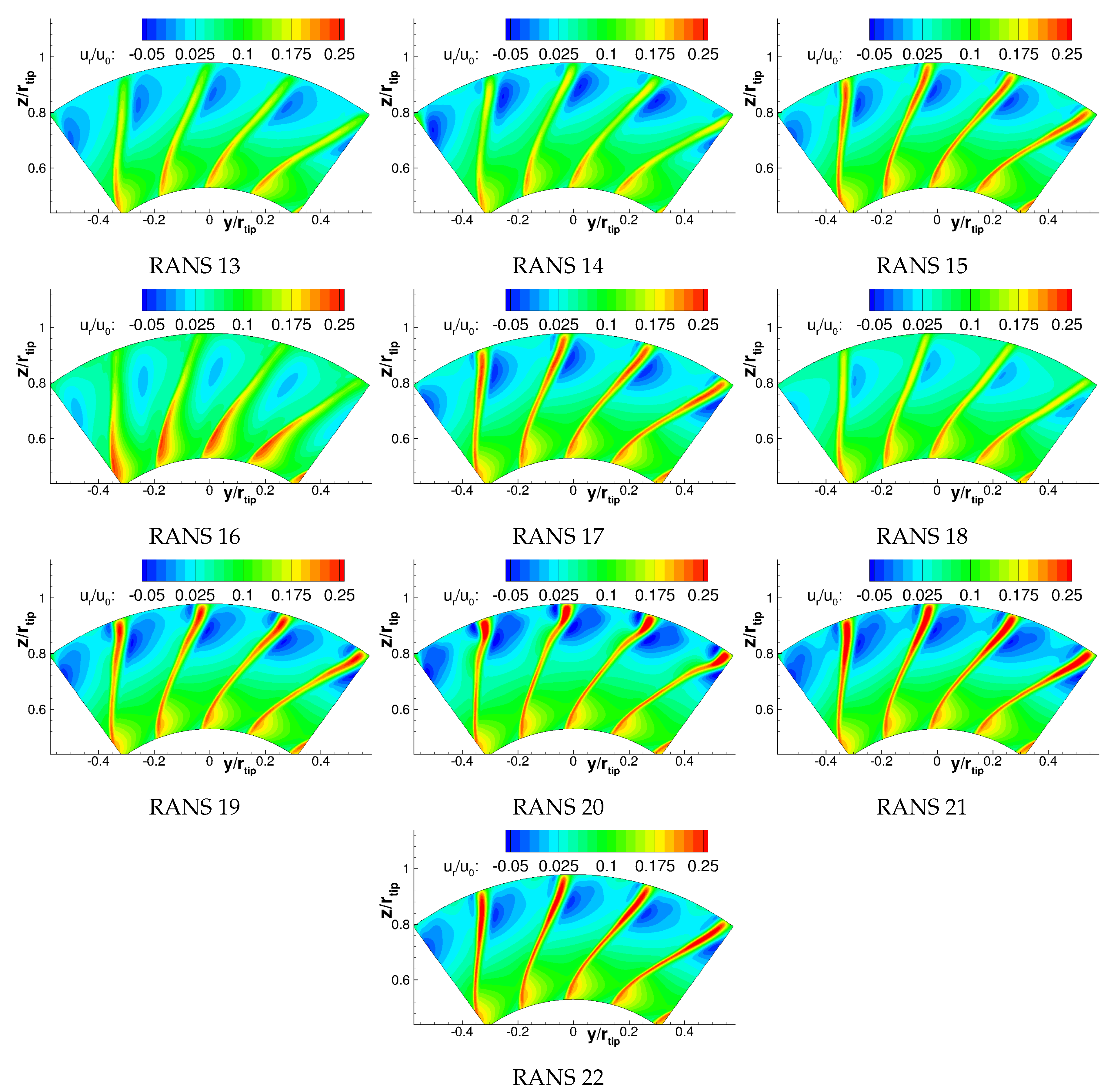
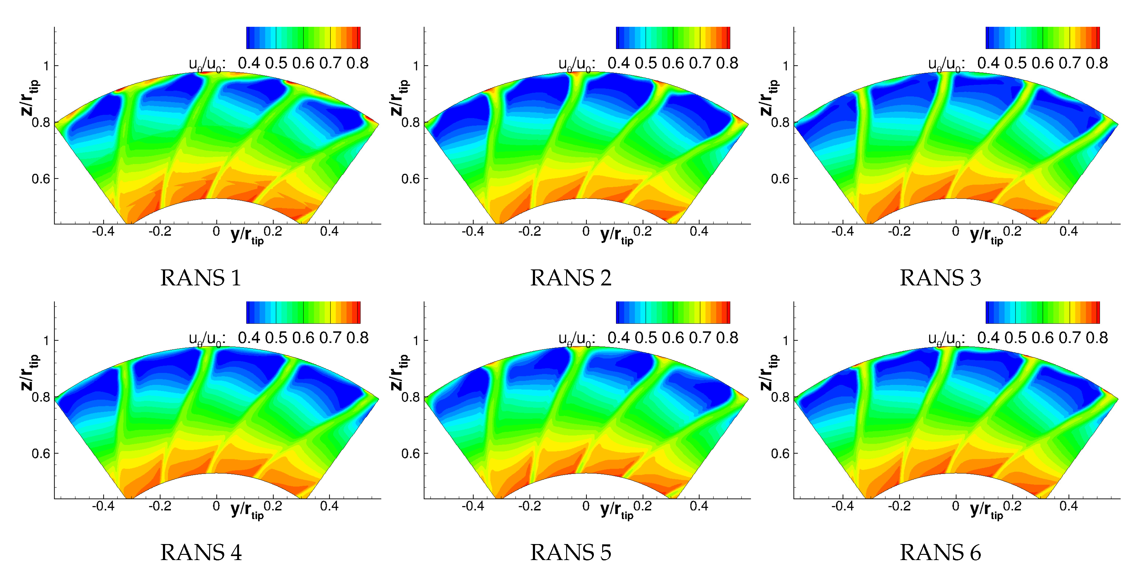
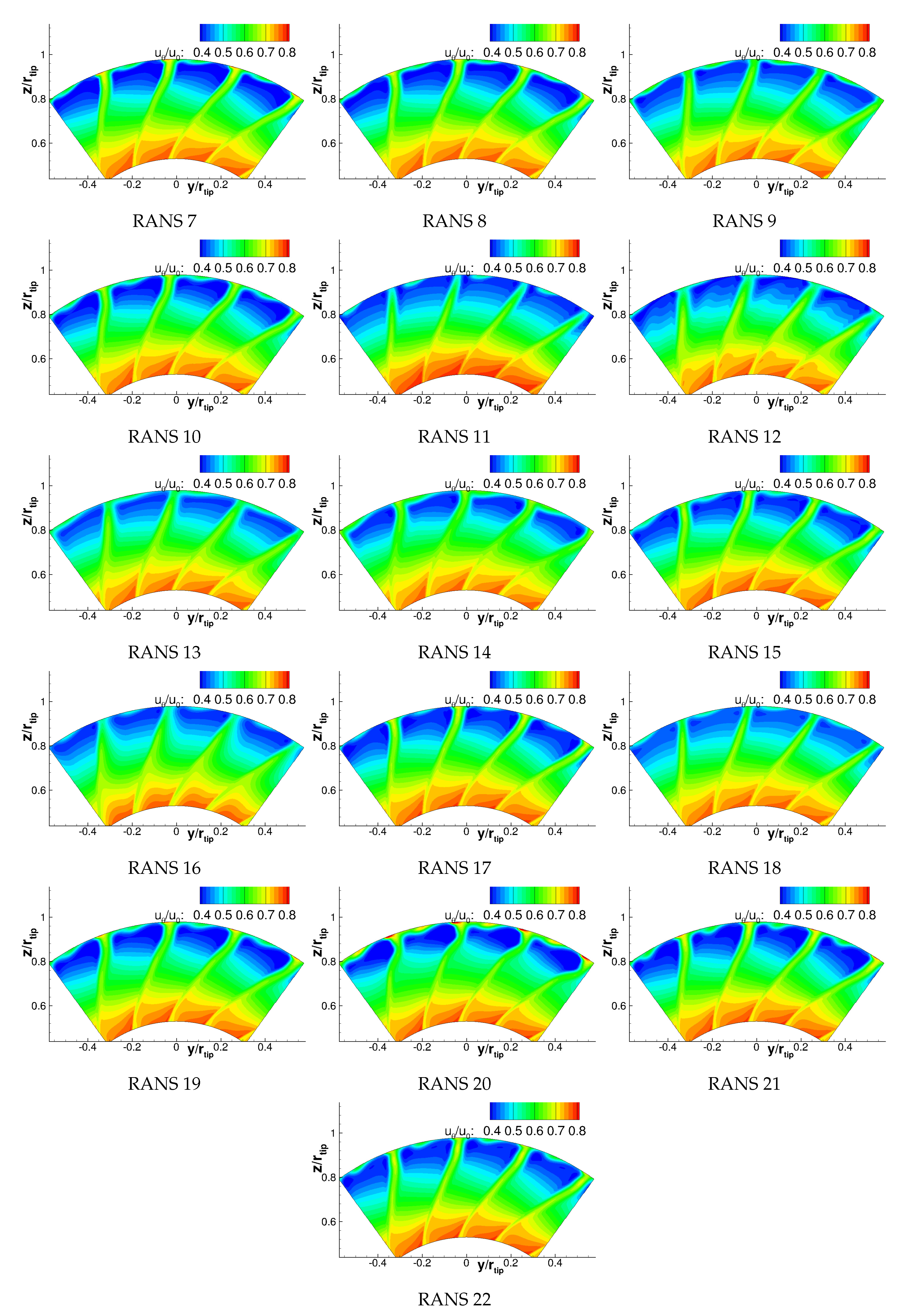
Appendix A. Velocities


Appendix B. Turbulence Characteristics


References
- Guérin, S.; Kissner, C.; Seeler, P.; Blazquez Navarro, R.A.; Carrasco Laraña, P.; de Laborderie, H.; Lewis, D.; Paruchuri, C.; Polacsek, C.; Thisse, J. ACAT1 Benchmark of RANS-informed Analytical Methods for Fan Broadband Noise Prediction: Part II—Influence of the Acoustic Models. Acoustics 2020. in review. [Google Scholar]
- Guérin, S.; Kissner, C.A.; Kajasa, B.; Jaron, R.; Behn, M.; Pardowitz, B.; Tapken, U.; Hakansson, S.; Meyer, R.; Enghardt, L. Noise prediction of the ACAT1 fan with a RANS-informed analytical method: Success and challenge. In Proceedings of the 25th AIAA/CEAS Aeroacoustics Conference, Delft, The Netherlands, 20–23 May 2019. [Google Scholar] [CrossRef]
- Grace, S.; Maunus, J.; Sondak, D.L. Effect of CFD Wake Prediction in a Hybrid Simulation of Fan Broadband Interaction Noise. In Proceedings of the 17th AIAA/CEAS Aeroacoustics Conference, Portland, OR, USA, 5–8 June 2011. [Google Scholar] [CrossRef]
- Maunus, J.; Grace, S.; Sondak, D.; Yakhot, V. Characteristics of turbulence in a turbofan stage. J. Turbomach. 2013, 135. [Google Scholar] [CrossRef]
- Ventres, C.S.; Theobald, M.A.; Mark, W.D. Turbofan Noise Generation. Volume 1: Analysis; Technical Report; Bolt Beranek and Newman Inc./NASA: Cleveland, OH, USA, 1982.
- Nallasamy, M.; Envia, E. Computation of rotor wake turbulence noise. J. Sound Vib. 2005, 282, 649–678. [Google Scholar] [CrossRef]
- Jaron, R.; Herthum, H.; Franke, M.; Moreau, A.; Guérin, S. Impact of Turbulence Models on RANS-Informed Predicition of Fan Broadband Interaction Noise. In Proceedings of the 12th European Turbomachinery Conference (ETC), Stockholm, Sweden, 3–7 April 2017. [Google Scholar]
- Jaron, R. Aeroakustische Auslegung von Triebwerksfans mittels multidisziplinärer Optimierungen. Ph.D. Thesis, TU Berlin, Berlin, Germany, 2018. [Google Scholar] [CrossRef]
- Moreau, A. A Unified Analytical Approach for the Acoustic Conceptual Design of Fans of Modern Aero-Engines. Ph.D. Thesis, TU Berlin, Berlin, Germany, 2017. [Google Scholar] [CrossRef]
- Meyer, R.; Hakansson, S.; Hage, W.; Enghardt, L. Instantaneous flow field measurements in the interstage section between a fan and the outlet guiding vanes at different axial positions. In Proceedings of the 13th European Conference on Turbomachinery Fluid Dynamics and Thermodynamics, Lausanne, Switzerland, 8–12 April 2019. [Google Scholar]
- Tapken, U.; Pardowitz, B.; Behn, M. Radial mode analyis of fan broadband noise. In Proceedings of the 2017, 23rd AIAA/CEAS Aeroacoustics Conference, Denver, CO, USA, 5–9 April 2017. [Google Scholar] [CrossRef]
- Behn, M.; Pardowitz, B.; Tapken, U. Separation of tonal and broadband noise components by cyclostationary analysis of the modal sound field in a low-speed fan test rig. In Proceedings of the Fan2018, Darmstadt, Germany, 18–20 April 2018. [Google Scholar]
- Joseph, P.; Morfey, C.L.; Lowis, C.R. Multi-mode sound transmission in ducts with flow. J. Sound Vib. 2003, 264, 523–544. [Google Scholar] [CrossRef]
- Tapken, U.; Behn, M.; Spitalny, M.; Pardowitz, B. Radial mode breakdown of the ACAT1 fan broadband noise generation in the bypass duct using a sparse sensor array. In Proceedings of the 25th AIAA/CEAS Aeroacoustics Conference, Delft, The Netherlands, 20–23 May 2019. [Google Scholar] [CrossRef]
- Behn, M.; Tapken, U. Investigation of Sound Generation and Transmission Effects Through the ACAT1 Fan Stage using Compressed Sensing-based Mode Analysis. In Proceedings of the 25th AIAA/CEAS Aeroacoustics Conference, Delft, The Netherlands, 20–23 May 2019. [Google Scholar] [CrossRef]
- Boussinesq, J. Essai sur la ThéOrie des eaux Courantes; Imprimerie Nationale: Paris, France, 1877. [Google Scholar]
- Hanjalić, K.; Jakirlić, S. A model of stress dissipation in second-moment closures. In Advances in Turbulence IV; Springer: Berlin/Heidelberg, Germany, 1993; pp. 513–518. [Google Scholar] [CrossRef]
- Wilcox, D.C. Turbulence Modeling for CFD; DCW Industries, Inc.: La Cañada Flintridge, CA, USA, 2006; Volume 3. [Google Scholar]
- Wilcox, D.C. Reassessment of the scale-determining equation for advanced turbulence models. AIAA J. 1988, 26, 1299–1310. [Google Scholar] [CrossRef]
- Menter, F.R. Two-equation eddy-viscosity turbulence models for engineering applications. AIAA J. 1994, 32, 1598–1605. [Google Scholar] [CrossRef]
- Menter, F.R.; Kuntz, M.; Langtry, R. Ten years of industrial experience with the SST turbulence model. Turbul. Heat Mass Transf. 2003, 4, 625–632. [Google Scholar]
- Smith, B. A near wall model for the k-l two equation turbulence model. In Proceedings of the Fluid Dynamics Conference, Colorado Springs, CO, USA, 20–23 June 1994. [Google Scholar] [CrossRef]
- Smith, B. A nonequilibrium turbulent viscosity function for the kl two equation turbulence model. In Proceedings of the 28th Fluid Dynamics Conference, Snowmass Village, CO, USA, 29 June–2 July 1997. [Google Scholar] [CrossRef]
- Hellsten, A. New Advanced k-w Turbulence Model for High-Lift Aerodynamics. AIAA J. 2005, 43, 1857–1869. [Google Scholar] [CrossRef]
- Launder, B.E.; Reece, G.J.; Rodi, W. Progress in the development of a Reynolds-stress turbulence closure. J. Fluid Mech. 1975, 68, 537–566. [Google Scholar] [CrossRef]
- Durbin, P.A. On the k-3 stagnation point anomaly. Int. J. Heat Fluid Flow 1996, 17, 9–90. [Google Scholar] [CrossRef]
- Menter, F.R.; Langtry, R.B.; Likki, S.R.; Suzen, Y.B.; Huang, P.G.; Völker, S. A correlation-based transition model using local variables—Part I: Model formulation. J. Turbomach. 2006, 128, 413–422. [Google Scholar] [CrossRef]
- Speziale, C.G.; Sarkar, S.; Gatski, T.B. Modelling the pressure–strain correlation of turbulence: An invariant dynamical systems approach. J. Fluid Mech. 1991, 227, 245–272. [Google Scholar] [CrossRef]
- Cécora, R.D.; Radespiel, R.; Eisfeld, B.; Probst, A. Differential Reynolds-stress modeling for aeronautics. AIAA J. 2015, 53, 739–755. [Google Scholar] [CrossRef]
- Hanjalić, K.; Jakirlić, S. Contribution towards the second-moment closure modelling of separating turbulent flows. Comput. Fluids 1998, 27, 137–156. [Google Scholar] [CrossRef]
- Jakirlić, S.; Hanjalić, K. A new approach to modelling near-wall turbulence energy and stress dissipation. J. Fluid Mech. 2002, 459, 139–166. [Google Scholar] [CrossRef]
- Jakirlić, S. A DNS-Based Scrutiny of RANS Approaches and Their Potential for Predicting Turbulent Flows; Postdoctoral Lecture Qualification; TU Darmstadt: Darmstadt, Germany, 2004. [Google Scholar]
- Jovanović, J.; Ye, Q.Y.; Durst, F. Statistical interpretation of the turbulent dissipation rate in wall-bounded flows. J. Fluid Mech. 1995, 293, 321–347. [Google Scholar] [CrossRef]
- Morsbach, C. Reynolds Stress Modelling for Turbomachinery Flow Applications. Ph.D. Thesis, Technische Universität Darmstadt, Darmstadt, Germany, 2016. [Google Scholar]
- Donzis, D.A.; Sreenivasan, K.R.; Yeung, P. Scalar dissipation rate and dissipative anomaly in isotropic turbulence. J. Fluid Mech. 2005, 532, 199–216. [Google Scholar] [CrossRef]
- Pope, S.B. Turbulent Flows; Cambridge University Press: Cambridge, UK, 2001. [Google Scholar] [CrossRef]
- Kissner, C.A.; Guérin, S. Influence of Wake and Background Turbulence on Predicted Fan Broadband Noise. AIAA J. 2019, 58, 659–672. [Google Scholar] [CrossRef]
- Wohlbrandt, A.; Kissner, C.; Guérin, S. Impact of cyclostationarity on fan broadband noise prediction. J. Sound Vib. 2018, 420, 142–164. [Google Scholar] [CrossRef]
- Ganz, U.W.; Joppa, P.D.; Patten, T.J.; Scharpf, D. Boeing 18-Inch Fan Rig Broadband Noise Test; Technical Report; NASA: Hamption, VA, USA, 1998. [Google Scholar]
- Lewis, D.; Moreau, S.; Jacob, M.C. On the Use of RANS-informed Analytical Models to Perform Broadband Rotor-Stator Interaction Noise Predictions. In Proceedings of the 25th AIAA/CEAS Aeroacoustics Conference, Delft, The Netherlands, 20–23 May 2019. [Google Scholar] [CrossRef]
- Becker, K.; Heitkamp, K.; Kügeler, E. Recent Progress in a Hybrid Grid CFD Solver for Turbomachinery Flows. In Proceedings of the V European Conference on Computational Fluid Dynamics ECCOMAS CFD 2010, Lisbon, Portugal, 14–17 June 2010. [Google Scholar]
- Cambier, L.; Heib, S.; Plot, S. The Onera elsA CFD software: Input from research and feedback from industry. Mech. Ind. 2013, 14, 159–174. [Google Scholar] [CrossRef]
- ANSYS, Inc. ANSYS CFX-Solver Theory Guide; ANSYS, Inc.: Canonsburg, PA, USA, 2011. [Google Scholar]
- Eriksson, L.E. Development and Validation of Highly Modular Flow Solver Versions in G2DFLOW and G3DFLOW; Technical Report; Volvo Aero Corporation: Trollhättan, Sweden, 1995. [Google Scholar]
- Corral, R.; Crespo, J.; Gisbert, F. Parallel multigrid unstructured method for the solution of the navier-stokes equations. In Proceedings of the 42nd AIAA Aerospace Sciences Meeting and Exhibit, Reno, NV, USA, 5–8 January 2004. [Google Scholar] [CrossRef]
- Gisbert, F.; Corral, R.; Pastor, G. Implementation of an Edge-Based Navier-Stokes Solver for Unstructured Grids in Graphics Processing Units. In Proceedings of the ASME Turbo Expo, Vancouver, BC, Canada, 6–10 June 2011; pp. 1375–1385. [Google Scholar] [CrossRef]
- Moinier, P. Algorithm Developments for an Unstructured Viscous Flow Solver. Ph.D. Thesis, Oxford University, Oxford, UK, 1999. [Google Scholar]
- Prasad, A.; Prasad, D. Unsteady Aerodynamics and Aeroacoustics of a High-Bypass Ratio Fan Stage. J. Turbomach. 2005, 127, 64–75. [Google Scholar] [CrossRef]
- Arroyo, C.P.; Leonard, T.; Sanjose, M.; Moreau, S.; Duchaine, F. Large Eddy Simulation of a scale-model turbofan for fan noise source diagnostic. J. Sound Vib. 2019. [Google Scholar] [CrossRef]
- François, B.; Barrier, R.; Polacsek, C. Zonal Detached Eddy Simulation of the Fan-OGV Stage of a Modern Turbofan Engine. In Proceedings of the ASME TurboExpo, London, UK, 21–25 September 2020. [Google Scholar]
- Polacsek, C.; Daroukh, M.; François, B.; Barrier, R. Turbofan Broadband Noise Predictions Based on a ZDES Calculation of a Fan-OGV Stage. In Proceedings of the Forum Acusticum, Lyon, France, 7–11 December 2020. [Google Scholar]
- Lewis, D.; Moreau, S.; Jacob, M. Broadband Noise Predictions on the ACAT1 Fan Stage Using Large Eddy Simulations and Analytical Models. In Proceedings of the 26th AIAA/CEAS Aeroacoustics Conference, Reno, NV, USA, 15–19 June 2020. [Google Scholar]
- Kissner, C.A.; Guérin, S.; Behn, M. Assessment of a 2D Synthetic Turbulence Method for Predicting the ACAT1 Fan’s Broadband Noise. In Proceedings of the 25th AIAA/CEAS Aeroacoustics Conference, Delft, The Netherlands, 20–23 May 2019. [Google Scholar] [CrossRef]
- Cader, A.; Polacsek, C.; Garrec, T.L.; Barrier, R.; Benjamin, F.; Jacob, M.C. Numerical prediction of rotor-stator interaction noise using 3D CAA with synthetic turbulence injection. In Proceedings of the 24th AIAA/CEAS Aeroacoustics Conference, Atlanta, GA, USA, 25–29 June 2018. [Google Scholar] [CrossRef]
- Polacsek, C.; Cader, A.; Barrier, R. Aeroacoustic design and broadband noise predictions of a turbofan stage with serrated outlet guide vanes. In Proceedings of the 26th International Congress on Sound and Vibration, Montreal, QC, Canada, 7–11 July 2019. [Google Scholar]
- Kissner, C.; Guérin, S. Fan Broadband Noise Prediction for the ACAT1 Fan Using a Three-Dimensional Random Particle Mesh Method. In Proceedings of the 26th AIAA/CEAS Aeroacoustics Conference, Reno, NV, USA, 15–19 June 2020. [Google Scholar]


| Turbulence | Turbulence Model | ||
|---|---|---|---|
| RANS | Solver | Model | Extensions |
| 1, 2 | TRACE [41] | Menter SST k- | none |
| 3, 5, 8 | elsA [42] | Menter SST k- | none |
| 4, 7 | ANSYS CFX v19.2 / v19.1 [43] | Menter SST k- | none |
| 6 | G3D::Flow [44] | Menter SST k- | none |
| 9 | [45,46] | Menter SST k- | Kato-Launder mod. |
| 10 | TRACE | Menter SST k- with Vorticity Source Term | none |
| 11 | TRACE | Menter SST k- | Kato-Launder mod. modified vortex extension (rotational fix) |
| 12 | HYDRA [47] | Menter SST k- | modifications for turbulent Mach number, rotation, low Re etc. |
| 13 | Wilcox k- | Kato-Launder mod. | |
| 14 | Wilcox k- | Kato-Launder mod., transition model | |
| 15 | TRACE | Wilcox k- | Schwarz limiter |
| 16 | TRACE | Wilcox k- | Kato-Launder mod. |
| 17, 18 | elsA | Smith k-l | none |
| 19 | TRACE | Hellsten EARSM k- | none |
| 20 | TRACE | Wilcox stress- | none |
| 21 | TRACE | SSG/LRR- | none |
| 22 | TRACE | JH stress- | none |
| Bypass | Core | Inlet | Inlet | Ambient | Ambient | ||
|---|---|---|---|---|---|---|---|
| Fan | Mass | Mass | Turbulence | Turbulent | Pressure | Temperature | |
| RANS | RPM | Flow [kg/s] | Flow [kg/s] | Intensity [%] | Length Scale [m] | [hPa] | [K] |
| 1, 2, 4, 10, 15, 16, 19-22 | 3828.1 | 48.75 | 6.41 | 0.3 | 0.04 | 995.6 | 292.8 |
| 3 | 3828.2 | 49.02 | 6.37 | 1.0 | 6.4 × 10 | 995.6 | 292.8 |
| 5 | 3828.2 | 48.75 | 6.41 | 0.3 | - | 995.6 | 292.8 |
| 6 | 3828.1 | 48.76 | 6.39 | 1.0 | 0.01 | 995.6 | 292.8 |
| 7 | 3828.2 | 48.75 | 6.44 | 0.3 | 0.04 | 995.3 | 292.8 |
| 8 | 3828.3 | 48.72 | 6.43 | 0.23 | 0.01 | 995.3 | 292.8 |
| 9 | 3828.2 | 48.75 | 6.41 | 0.36 | 0.043 | 1013.25 | 288.15 |
| 11 | 3856.1 | 49.85 | 6.70 | 0.88 | 0.00018 | 1013.25 | 288.15 |
| 12 | 3828.1 | 49.10 | 6.45 | 0.30 | 0.04 | 995.3 | 292.8 |
| 13, 14 | 3828.2 | 48.75 | 6.41 | 0.36 | 0.043 | 1013.25 | 288.15 |
| 17 | 3828.2 | 48.75 | 6.41 | 0.3 | - | 995.6 | 292.8 |
| 18 | 3828.3 | 48.72 | 6.43 | 0.23 | 0.01 | 995.3 | 292.8 |
| Tip | Total | Azimuthal Wake | Boundary | Spatial | |
|---|---|---|---|---|---|
| Clearance | Mesh Size | Resolution | Layer | Discretization | |
| RANS | [mm] | [Mio. cells] | at R = 75% [cells] | Resolution | Scheme |
| 1, 10, 12, 15, 16, 19–22 | 0.78 | 6.5 | ≈30 | resolved | 2nd order |
| 2 | 0.78 | 4.8 | ≈20 | resolved | 2nd order |
| 3 | 0.63 | 63 | ≈30 | resolved | 3rd order |
| 4 | 0.78 | 70 | >25 | resolved | CFX high resolution |
| 5 | 0.78 | 4.5 | ≈30 | resolved | 2nd order |
| 6 | 0.78 | 15.4 | ≈20 | resolved | 3rd order convective, 2nd order diffusive |
| 7 | 0.63 | 7.0 | ≈20 | resolved | CFX high resolution |
| 8, 18 | 0.63 | 38.0 | ≈20 | resolved | 2nd order |
| 9, 13, 14 | 0.63 | 35.5 | ≈30 | wall functions (OGV), resolved (rotor) | 2nd order |
| 11 | 0.58 (LE) 0.69 (TE) | 11.3 | ≈15 | resolved | 2nd order |
| 17 | 0.78 | 4.5 | ≈30 | resolved | 2nd order |
© 2020 by the authors. Licensee MDPI, Basel, Switzerland. This article is an open access article distributed under the terms and conditions of the Creative Commons Attribution (CC BY) license (http://creativecommons.org/licenses/by/4.0/).
Share and Cite
Kissner, C.; Guérin, S.; Seeler, P.; Billson, M.; Chaitanya, P.; Carrasco Laraña, P.; de Laborderie, H.; François, B.; Lefarth, K.; Lewis, D.; et al. ACAT1 Benchmark of RANS-Informed Analytical Methods for Fan Broadband Noise Prediction—Part I—Influence of the RANS Simulation. Acoustics 2020, 2, 539-578. https://doi.org/10.3390/acoustics2030029
Kissner C, Guérin S, Seeler P, Billson M, Chaitanya P, Carrasco Laraña P, de Laborderie H, François B, Lefarth K, Lewis D, et al. ACAT1 Benchmark of RANS-Informed Analytical Methods for Fan Broadband Noise Prediction—Part I—Influence of the RANS Simulation. Acoustics. 2020; 2(3):539-578. https://doi.org/10.3390/acoustics2030029
Chicago/Turabian StyleKissner, Carolin, Sébastien Guérin, Pascal Seeler, Mattias Billson, Paruchuri Chaitanya, Pedro Carrasco Laraña, Hélène de Laborderie, Benjamin François, Katharina Lefarth, Danny Lewis, and et al. 2020. "ACAT1 Benchmark of RANS-Informed Analytical Methods for Fan Broadband Noise Prediction—Part I—Influence of the RANS Simulation" Acoustics 2, no. 3: 539-578. https://doi.org/10.3390/acoustics2030029
APA StyleKissner, C., Guérin, S., Seeler, P., Billson, M., Chaitanya, P., Carrasco Laraña, P., de Laborderie, H., François, B., Lefarth, K., Lewis, D., Montero Villar, G., & Nodé-Langlois, T. (2020). ACAT1 Benchmark of RANS-Informed Analytical Methods for Fan Broadband Noise Prediction—Part I—Influence of the RANS Simulation. Acoustics, 2(3), 539-578. https://doi.org/10.3390/acoustics2030029