4.2. Wind Conditions and Atmospheric Conditions
A starting point for evaluation of the influence of atmospheric conditions on acoustic signals is an analysis of the measurement periods over several days. In
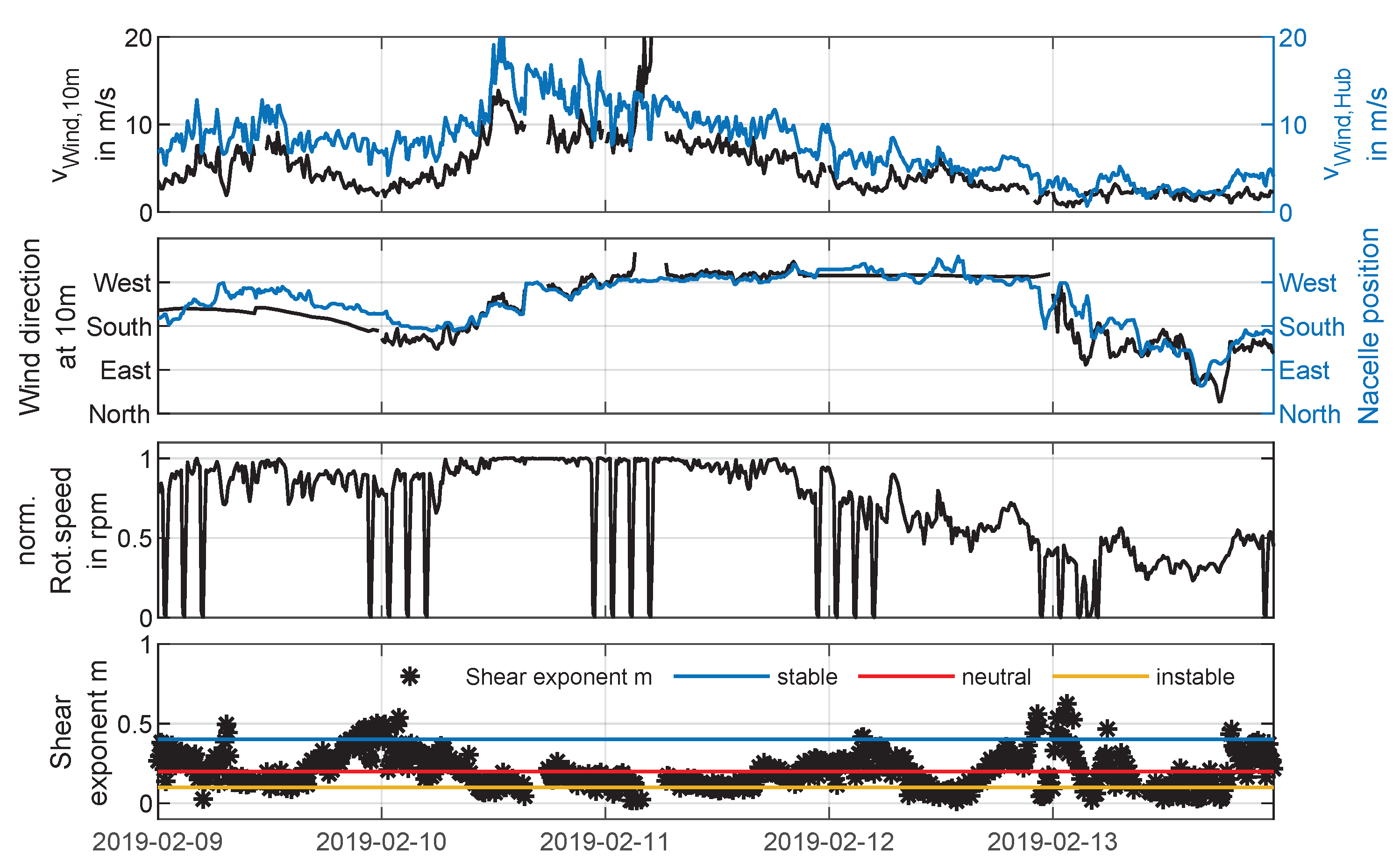
Figure 8, the 10 min averaged meteorological parameters over a measurement period of five days from 9 February 2019 to 13 February 2019 at Site 1 and location L2 are plotted. The wind speed and wind direction plot on the top show that both wind speed and wind direction measured at a 10 m height and hub height followed the same shape. In particular, the measured wind direction matched the provided data at hub height. The wind direction plot shows that measurement locations L2 and L3 were mainly crosswind from the WT during the first and last days as wind came from the south. During 11 February 2019 and 12 February 2019, position L2 was located in the downwind direction, whereas L3 was located upwind from the WT since the wind came from the western direction. The rotational speed plotted in rotations per minute (rpm) in the third plot was normalized to a maximum rotational speed. Time periods with zero rotation marked the 20 min shutdown periods during the night time. From the bottom plot, it is evident that stable atmospheric conditions mainly occurred during the night time (cf. [
24]). During time periods with high wind speeds at both considered heights (e.g., 11 February 2019 and 12 February 2019), mixed air layers led to an instable or neutral atmosphere, which was more likely during the daytime. The same applied to time periods with low wind speeds at both heights (e.g., 13 February 2019).
In
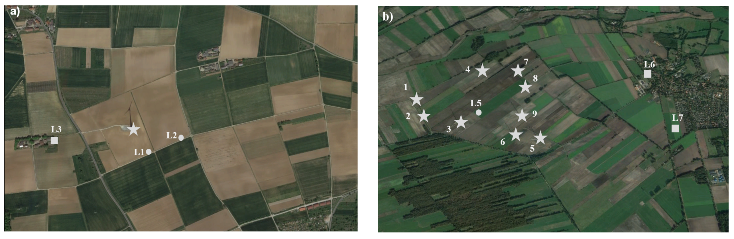
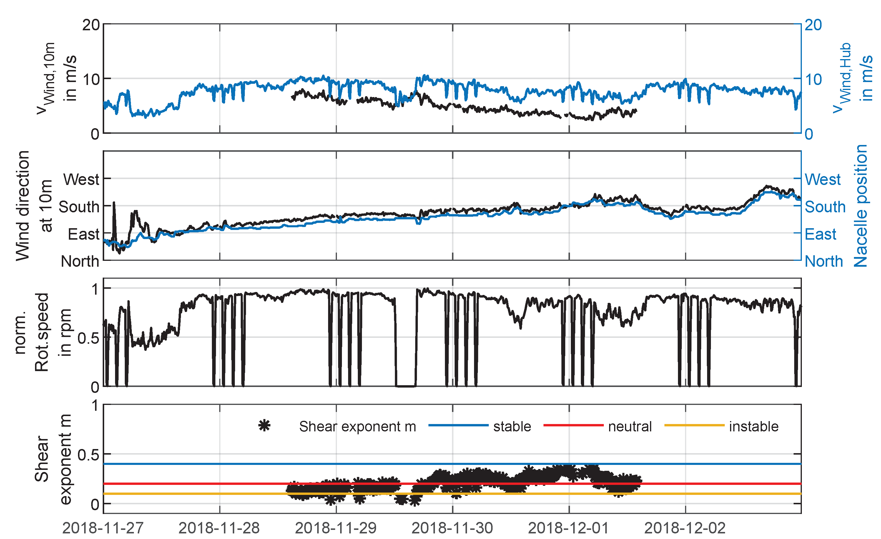
Figure 9, the same 10 min averaged parameters are plotted for a period of six days from 27 November 2018 to 2 December 2018 at Site 2, whereas data at a 10 m height were measured at location L5 and the data for hub height for WT3; see
Figure 1. Due to an anemometer malfunction, met-mast wind speed data were only available for three days within this week. As already seen from the measurements at Site 1, there was a good agreement between wind direction data measured at different heights, also in a wind park. The plot shows that measurement locations L6 and L7 were mainly crosswind from the WT as the wind came from the south most of the time. Considering WT3, which was closest to L5, the measurement location L5 was also crosswind from the WT. By comparing wind speed and rotational speed at hub height, it was obvious that shutdown times during nighttime influenced the measured wind speed. Additionally, it was also specified by the WT operator not to use wind speed data of shutdown periods. This needed to be considered when evaluating the shear exponent. This could be the reason that the difference between stable and instable conditions during day and night was not as clearly distinguishable as on February 2019. However, a stable atmosphere became apparent mainly during the night.
4.3. Time Series of Sound Pressure Data
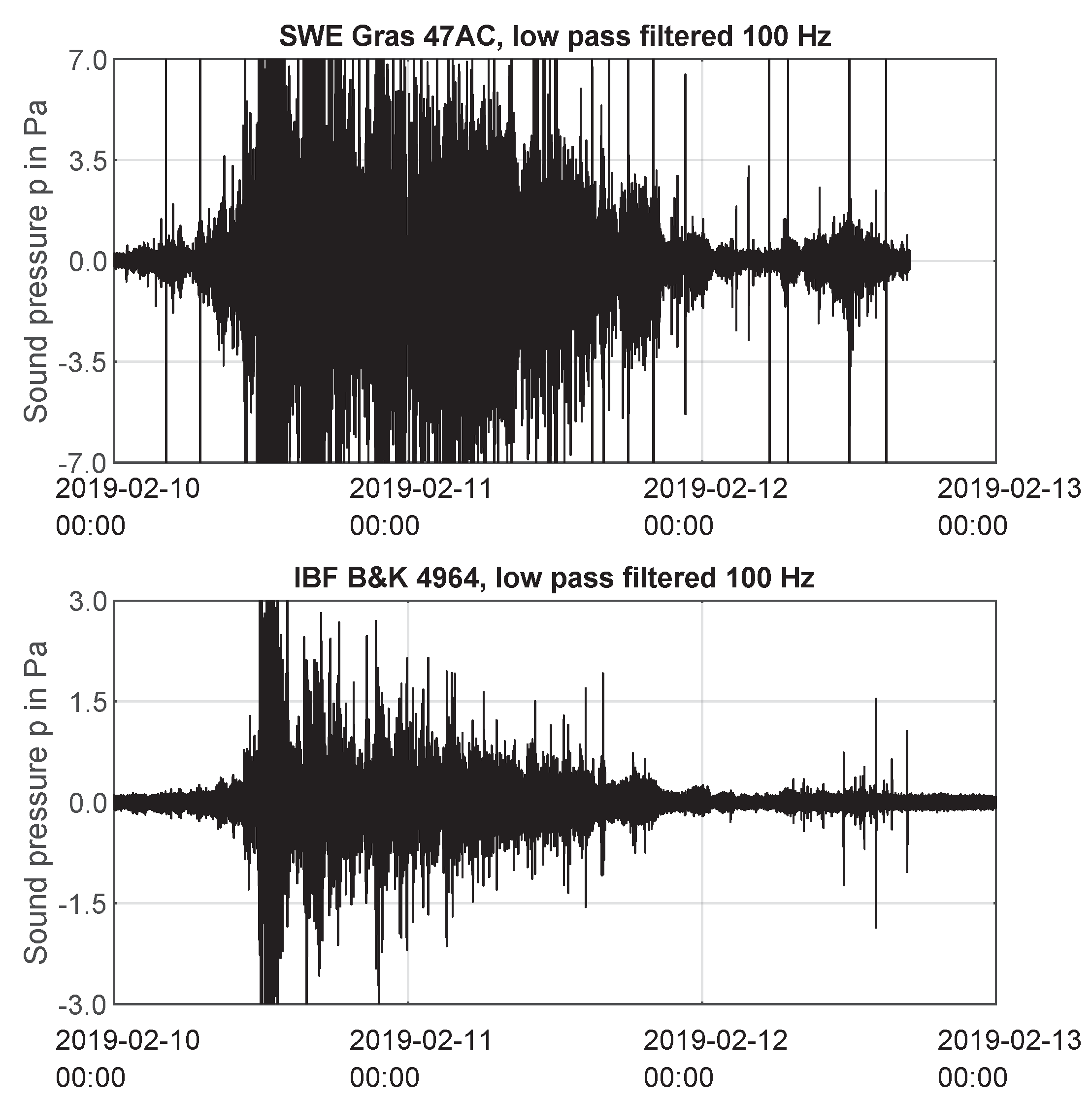
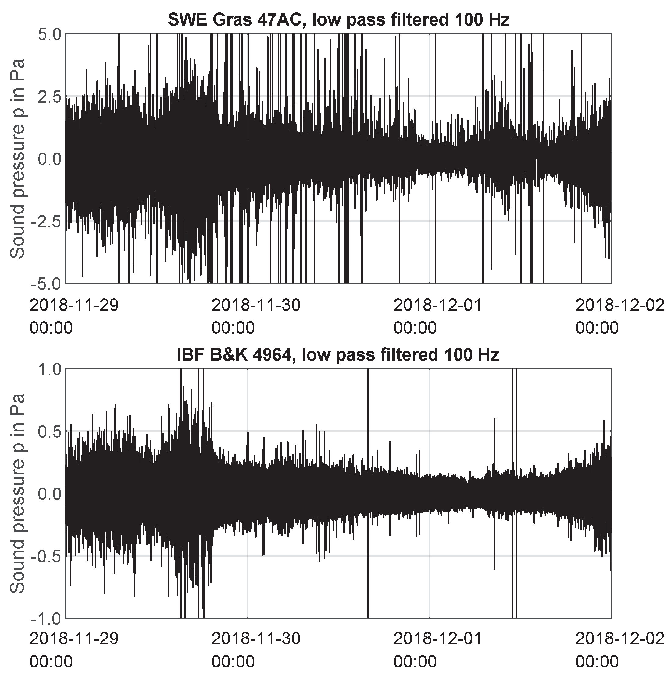
For the comparison of SWE and IBF measurements with the focus on low frequencies, the acoustic data were low-pass filtered with 100 Hz and plotted over time in
Figure 10 and
Figure 11. Three day time periods of measurements at Site 1 in February 2019 (SWE microphone malfunction on 12 February 2019 17:30) and at Site 2 in November 2019 are shown for a qualitative comparison.
As expected, the results showed that sound pressure amplitudes
p at the point of emission were significantly higher (partially twice or more) than sound pressure amplitudes inside of buildings. One of the main reasons for that was the acoustic noise produced by wind and its effects on the natural surroundings. Beside the reduced air movement in a more or less sheltered area, the amount of other anthropogenic noise sources was also reduced, especially during the absence of residents. Thus, IBF time series of
p in
Figure 10 and
Figure 11 showed less short-time peaks with clearly higher amplitudes. Altogether, there was a tendency that the time series of emission and immission coincided in a way that the form of an enveloping curve around the measured signals indicated simultaneous increases and decreases of the amplitudes.
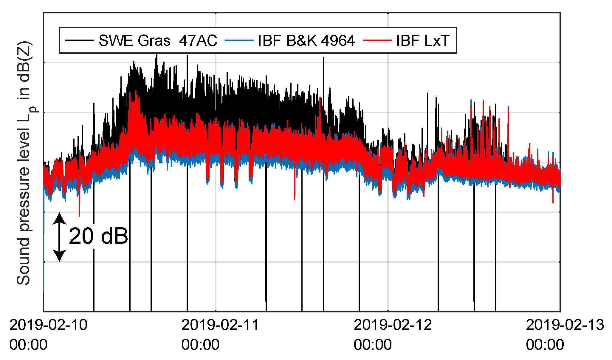
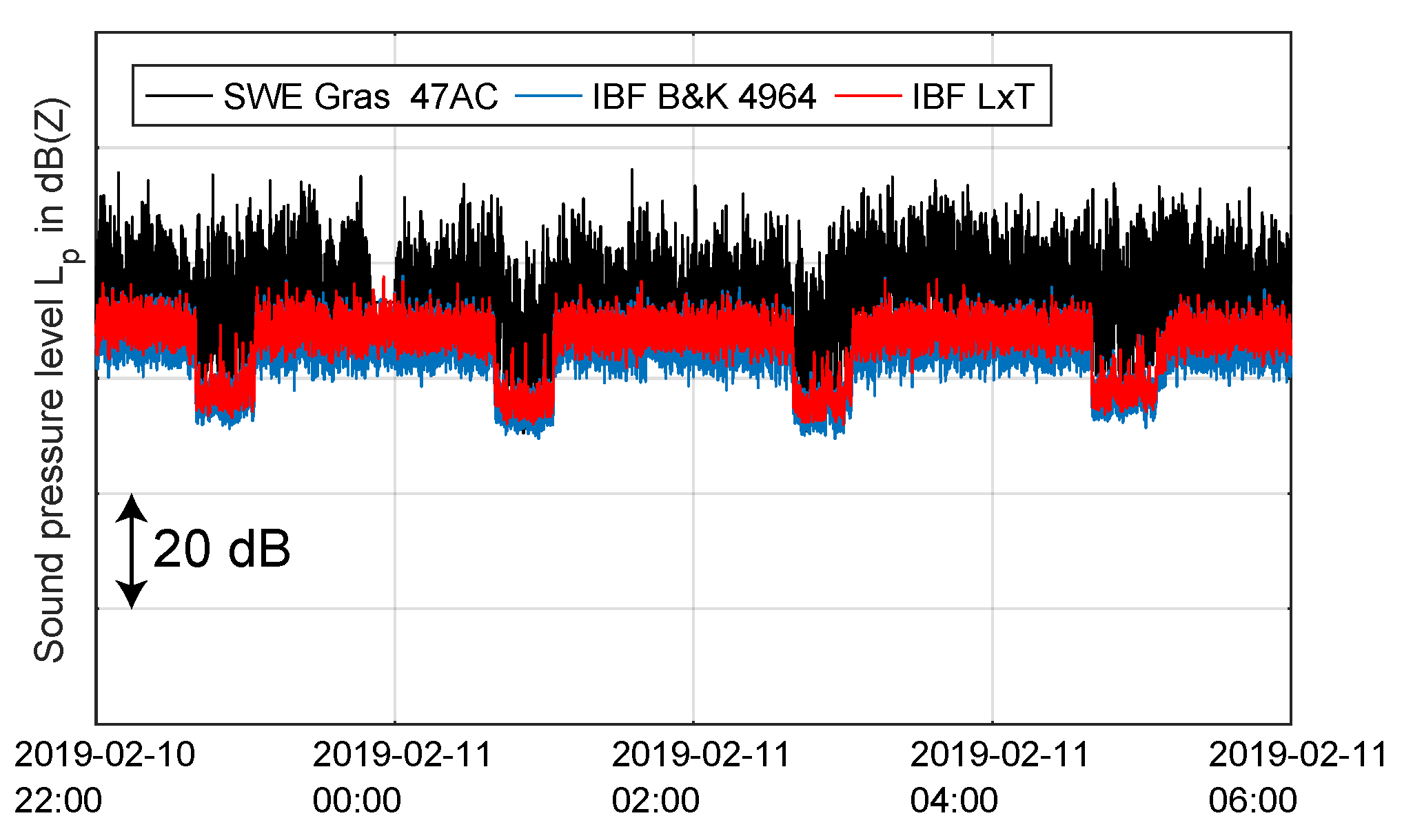
Both SWE and IBF time series data did not show a clear indication whether the wind turbine was operating or not. As noted in
Section 2.1, the WT was stopped at 00:40, 02:40, 04:40, and 22:40 (UTC) every day during the presented time periods. In contrast with the
time series, it was observed that the time series of the 10 s sound level pressure
(measured inside of the buildings with the Larson Davis SoundTrack LxT sound level meter) showed decreases of SPL during shutdown times. This could be confirmed, e.g., by
Figure 12 and
Figure 13, in which the red colored time series changes obviously for defined time periods. Based on bandpass filtered (5 Hz–100 Hz)
values of SWE and IBF data from
Figure 10 and
Figure 11, the SPL was calculated using Equation (
2) for both cases and also plotted in
Figure 12 and
Figure 13. This, on the one hand, offered the possibility to prove the plausibility of the IBF measurements with two independent measuring systems and, on the other hand, that shutdown times could be made visible. The SPL in the free field tended to be higher and more variable because of the enhanced influence from all kinds of surrounding acoustic noise sources. It is important to mention that the calculated SPL time series of SWE in
Figure 12 shows unrealistic zero values of
due to electrical disturbances caused by automatic switching of the UPS system used, mentioned in
Section 4.1.
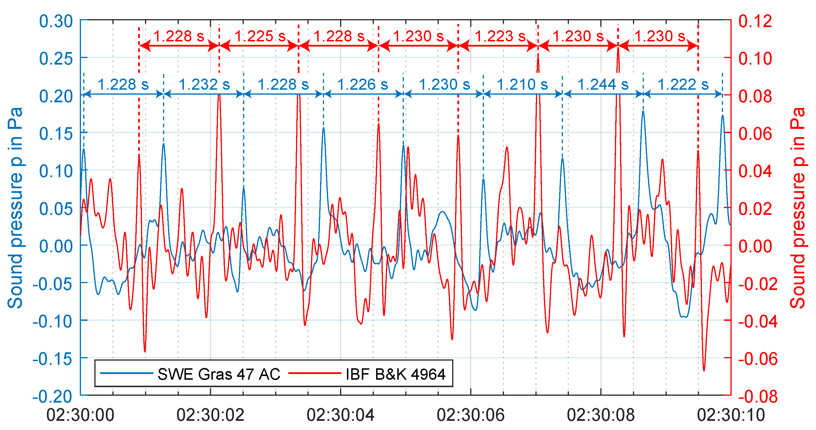
The impulsiveness of noise is often seen as critical because it favors the perceptibility of such acoustic emissions. In the case of WT noise, the passage of rotor blades in front of the tower caused this impulsive behavior, which can be seen in the time series of measured sound pressure data. As an example, sound pressure data of SWE and IBF for 10 February 2019 were bandpass filtered between 0.5 Hz and 10 Hz, and an arbitrary 10 s time sequence during the night (detailed view of
Figure 10) was chosen for the plot in
Figure 14. Each blade passage is clearly visible as a sharp peak of sound pressure in
Figure 14 both for measured data of SWE, as well as IBF. In both cases, the time difference between preceding and following peaks was about
, which resulted in a blade passing frequency of
, corresponding to a rotational speed of 16 rpm.
4.4. Time-Variant Spectral Representation
According to the approach described in
Section 3, time variant PSD plots of measured acoustic signals at Site 1 and 2 are presented in
Figure 15 and
Figure 16 for a frequency range from 0.1 Hz to 140 Hz.
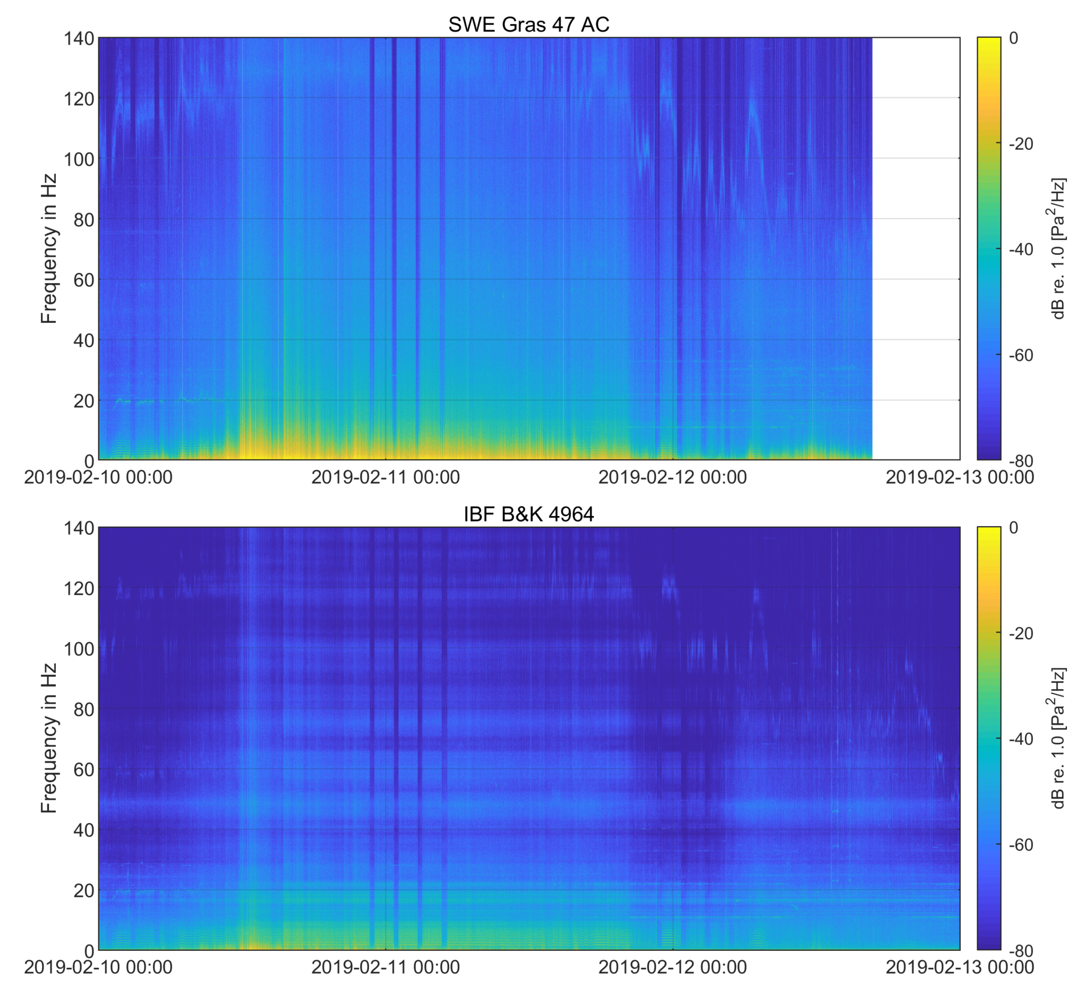
Detailed evaluation of
Figure 15 yielded that shutdown periods of the WT were clearly recognizable both at place of emission (L2) and place of immission (L3) in contrast to the
p-
t diagrams in
Figure 10. During WT shutdown, power spectral density was reduced over the full frequency range from about 0.5 Hz to 140 Hz, which is indicated through the color mapping. Of special interest for the determination of sources of low frequency acoustic noise produced by the WT were signal components that disappeared during shutdown. By regarding the first half of 10 February 2019 in
Figure 15, several signal components can be observed below 10 Hz, with a varying frequency around 20 Hz and with a strongly varying frequency between 100 Hz (partly even lower) and 130 Hz, which disappeared instantly when the rotational speed of the WT dropped to zero (see
Figure 8). The frequencies below 10 Hz (see
Figure 17 for details) mainly occurred during a stable atmosphere and appeared to be directly correlated with the rotational speed of the wind turbine as multiples of the blade passing frequency (BPF). A more detailed discussion of these signal components is presented in
Section 4.5.
Furthermore, it can be seen that the PSD intensity for the whole frequency range increased for higher wind speeds between 10 February 2019 12:00 (UTC) and 11 February 2019 21:00 (UTC). As the level decreased visibly during the shutdown times on the night of 11 February 2019, the broadband noise must be induced by the WT and was not induced by wind noise on the microphone level. This could be related to instable atmospheric conditions (see
Figure 8) occurring during the considered period, which led to a higher turbulent inflow of the rotor blades. Due to [
22], “in-flow turbulent sound” contributed to a broadband noise over a wide frequency range, which was less dominant during a stable atmosphere. Similar observations were made by [
25], who correlated turbulent inflow noise to turbulence intensity and proved it to be no wind induced background noise.
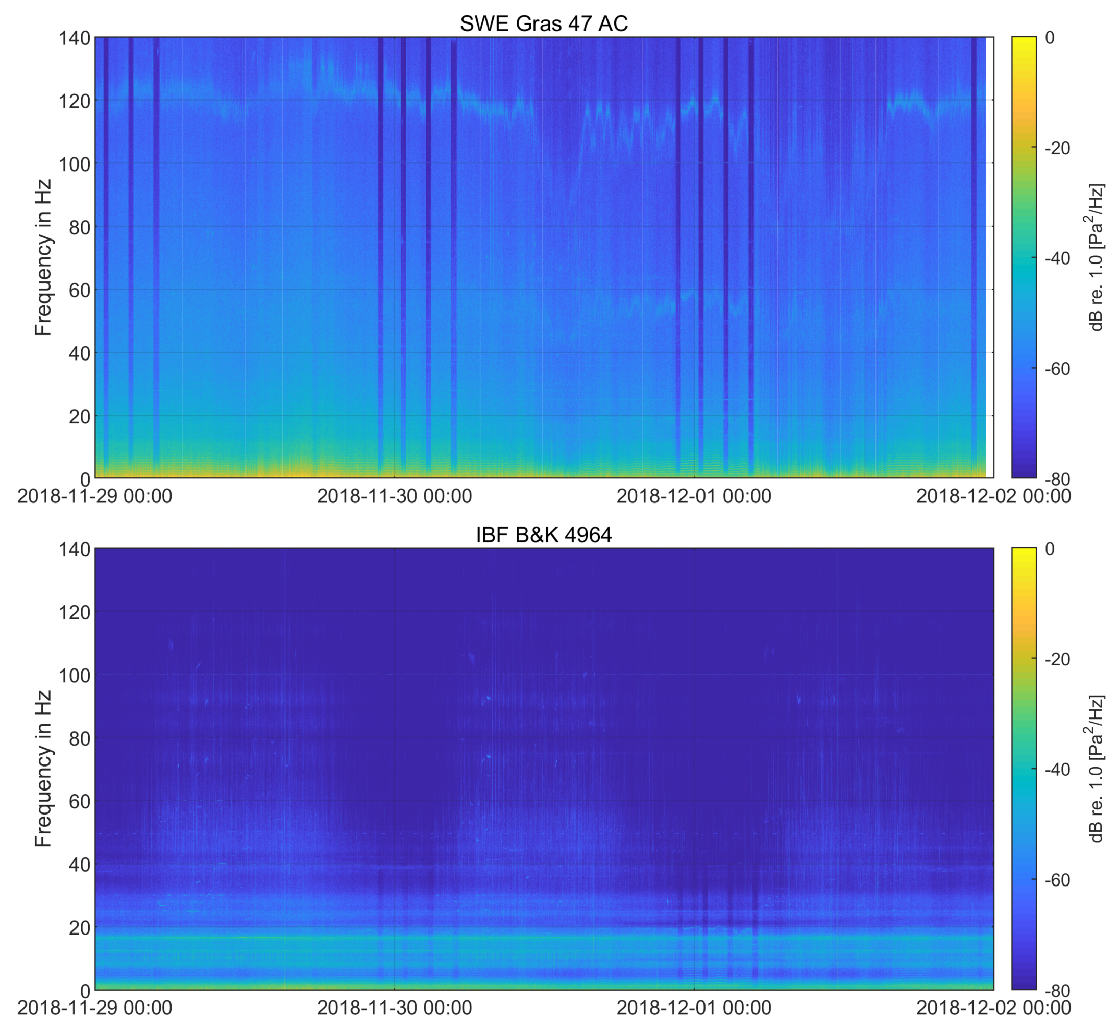
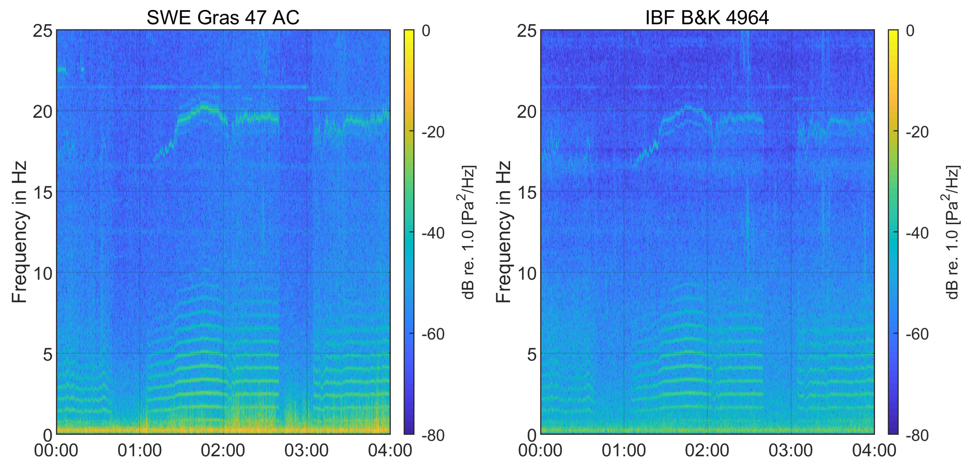
Figure 16 shows the spectrogram of acoustic data from Site 2 in northern Germany with nine wind turbines. Shutdown times of the wind farm are very clearly visible over the whole three day time period for the SWE measurements outside, and the intensity reduction was significant. Signal components below 10 Hz, around 20 Hz, 55 Hz, and 120 Hz had the highest intensities in the spectrogram, for example on 30 November 2019 at 00:00 (UTC) and 2018/12/01 at 00:00 (UTC). Inside of a building at location L6, shutdown times were only visible for frequencies below 40 Hz, and only several signal components below 10 Hz could be related to the wind farm. Other signals with frequencies of 12.8 Hz and 17.0 Hz were continuous and unaffected by WT operation.
4.5. Comparison of Sound Pressure Levels
For further analysis in the frequency range from 0.6 Hz to 120 Hz, spectra for selected 10 min periods were calculated according to
Section 3 for measurements on Site 1 in February 2019.
Figure 18 and
Figure 19 show the comparison between rotating (on) and still (off) WT for different atmospheric conditions, classified according to
Table 4. On periods where matched to off periods with mostly similar conditions concerning shear exponent
m, rotational number, nacelle position, and wind speed at a 10 m height. Detailed information for each time period is given in
Table 5.
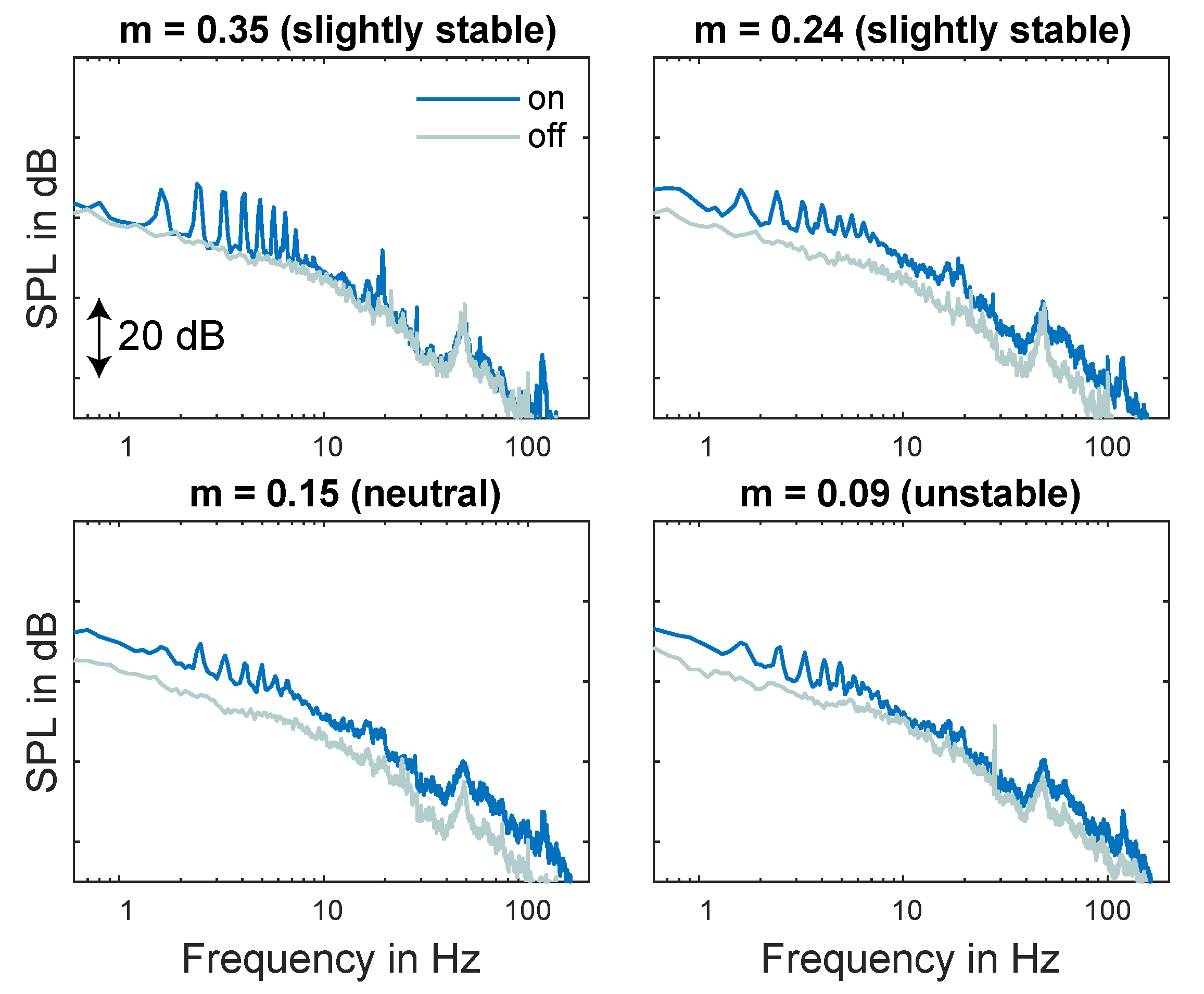
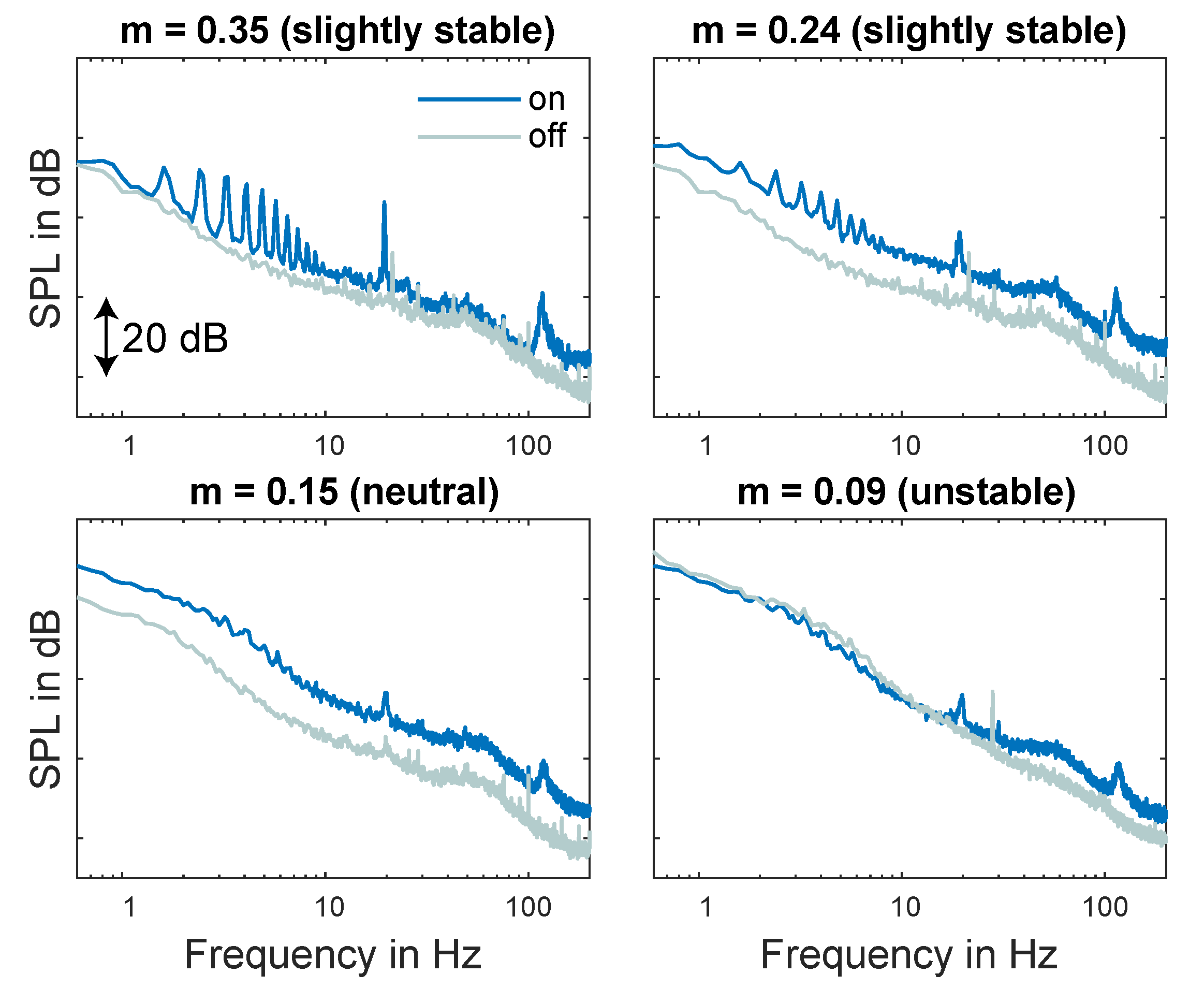
The main difference of the on/off spectra were tones below 10 Hz, around 20 Hz, and 120 Hz, which were identified in
Section 4.4 and
Figure 15. The outside spectra showed that during stable conditions, the BPF tones at 0.8 Hz and higher harmonics up to 10 Hz were the most dominant; whereas tones at 19 Hz and 117 Hz were also present for neutral and instable conditions. It was also visible that with decreasing shear exponent
to instable atmospheric conditions, the SPL of both background noise and WT noise was increasing. This resulted in a masking of BPF peaks below 10 Hz. The same frequencies could be identified inside at measurement location L3 (
Figure 19). The tones of the BPF were dominant with the stable condition, but in contrast to the outside spectra, still visible during the neutral and instable condition. A peak at 16.6 Hz may be a room mode, whereas the tone around 48 Hz, which was dominant during rotating, but also still WT was related to electric noise (probably a three phase asynchronous machine).
By comparing inside with outside measurements, a rough assumption of the decrease in SPL over distance was possible. Here, it must be taken into account that measurement locations L2 and L3 were located in opposite directions related to the WT, and the attenuation over distance was just an indication.
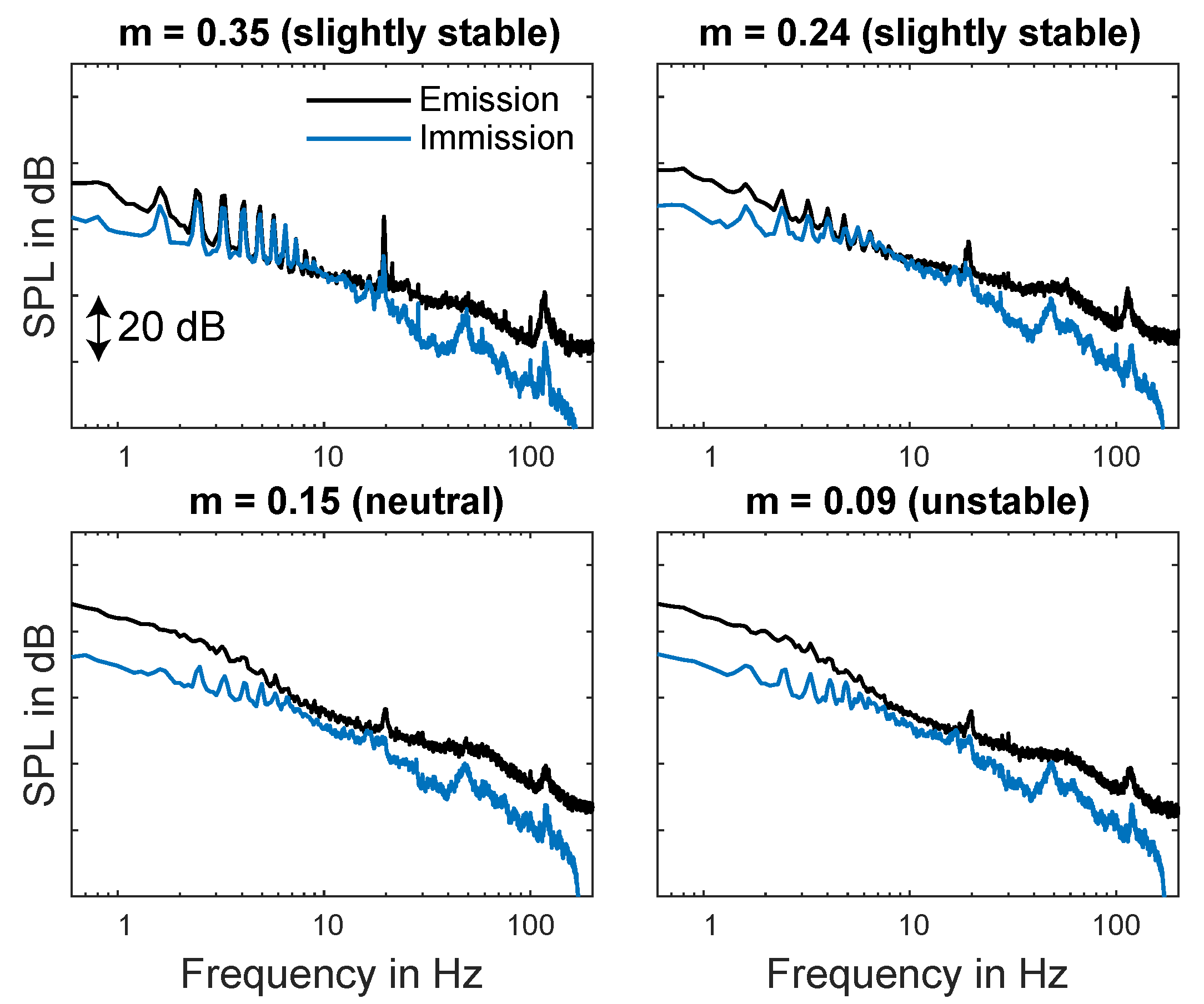
Figure 20 shows frequency spectra from
Figure 18 and
Figure 19 for different atmospheric conditions. Below 10 Hz, there was a maximum decrease in SPL from outside to inside of 5 dB at 0.8 Hz during stable conditions. For less stable conditions, the SPL difference between inside and outside increased due to increasing wind noise. It was also visible that BPF tones were more dominant inside during unstable conditions, since there was no masking by background noise. Furthermore, all four plots of
Figure 20 showed that there was no attenuation over distance for a frequency around 6 Hz. Besides a low air absorption in the low frequency range, there seemed to be no sound insulation by the facade. This was confirmed by [
4], who showed that due to the mass law, the outside-to-inside reduction of the facade had its minimum around 10 Hz.
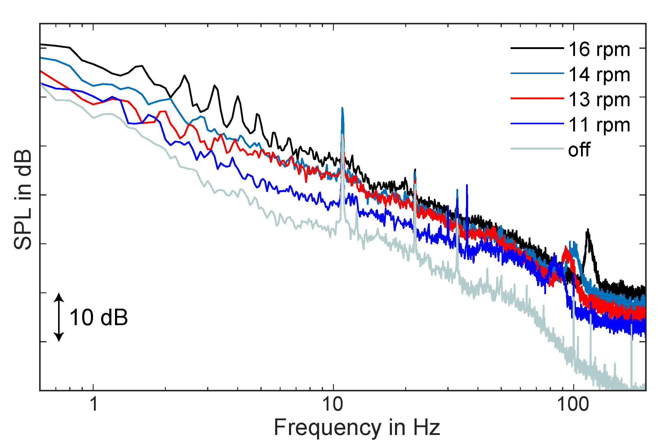
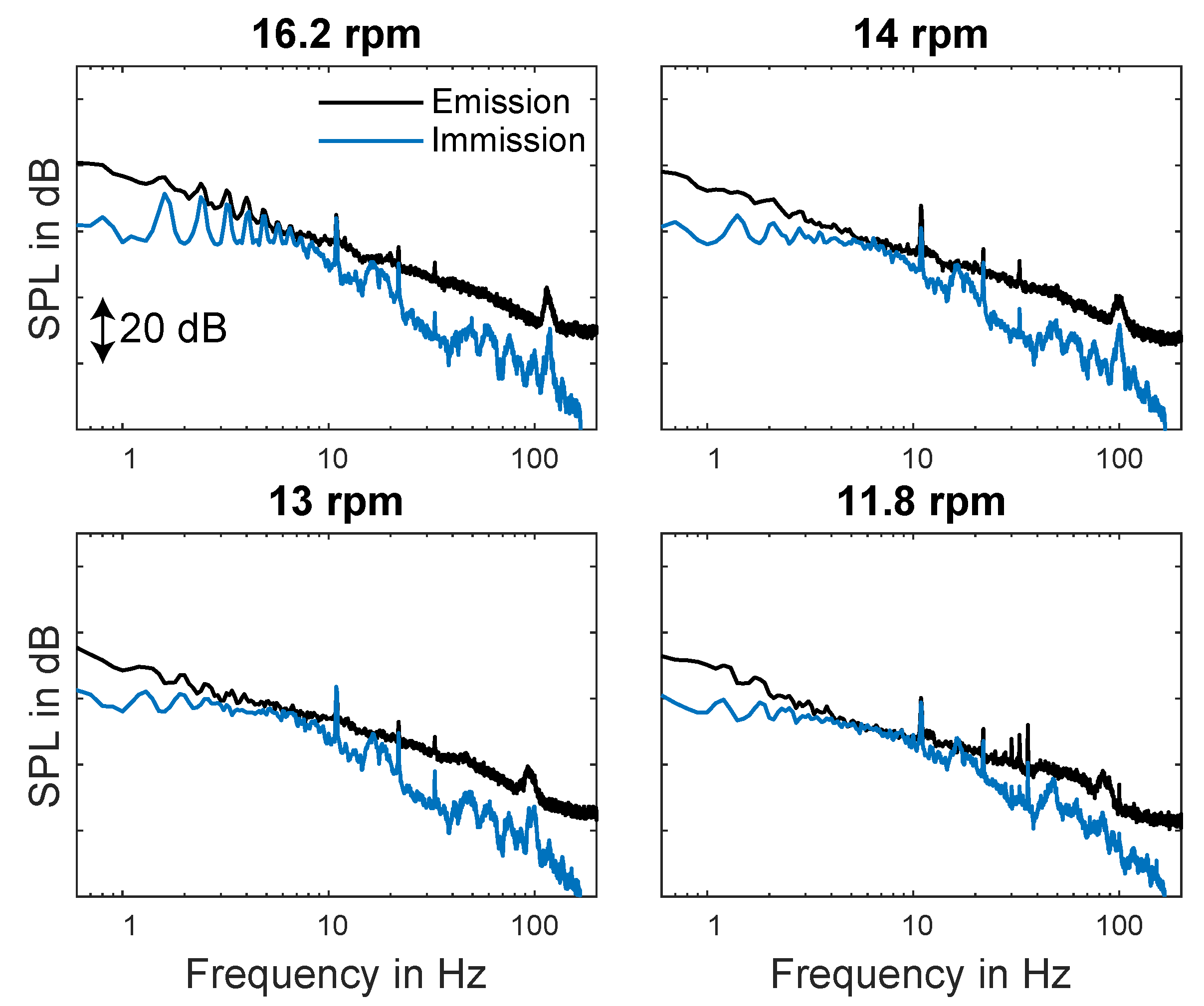
Furthermore, the influence of rotational speed and thus varying power output of the WT on acoustic signals was evaluated. Therefore, the spectra of 10 minute time periods on 12 February 2019 for different rotational speeds, but neutral atmospheric conditions, a similar wind speed at a 10 m height, and nacelle position were compared. Detailed information of each time period is listed in
Table 6. As expected, it can be seen in
Figure 21 that the rotational speed of the WT had an effect on the measured BPF in terms of frequency, as well as the dominance of the peaks. Thus, the strong variation of WT tones identified in
Figure 15 and
Figure 16 around 20 Hz and between 80 Hz and 130 Hz could be clearly related to a variation of rotational speed. A comparison between spectra measured outside and inside in
Figure 22 showed that BPF tones were most dominant with the highest rotational speed.
In many cases, acoustic noise is measured with the use of sound pressure level meters, which often means that only information about SPL and the frequency components of the signal are recorded and plotted in one-third octave spectra. To complement the results of the shown narrow-band spectra (
Figure 18,
Figure 19,
Figure 20,
Figure 21 and
Figure 22) obtained through direct measurements of sound pressure
, one-third octave spectra were generated according to
Section 3. This offered the possibility to insert a curve of the hearing threshold. For the considered frequency range between 1 Hz and 125 Hz, the threshold values were composed by two different literature sources. Frequencies below 8 Hz were proposed by [
23], and the frequency range between 8 Hz and 125 Hz was according to [
26].
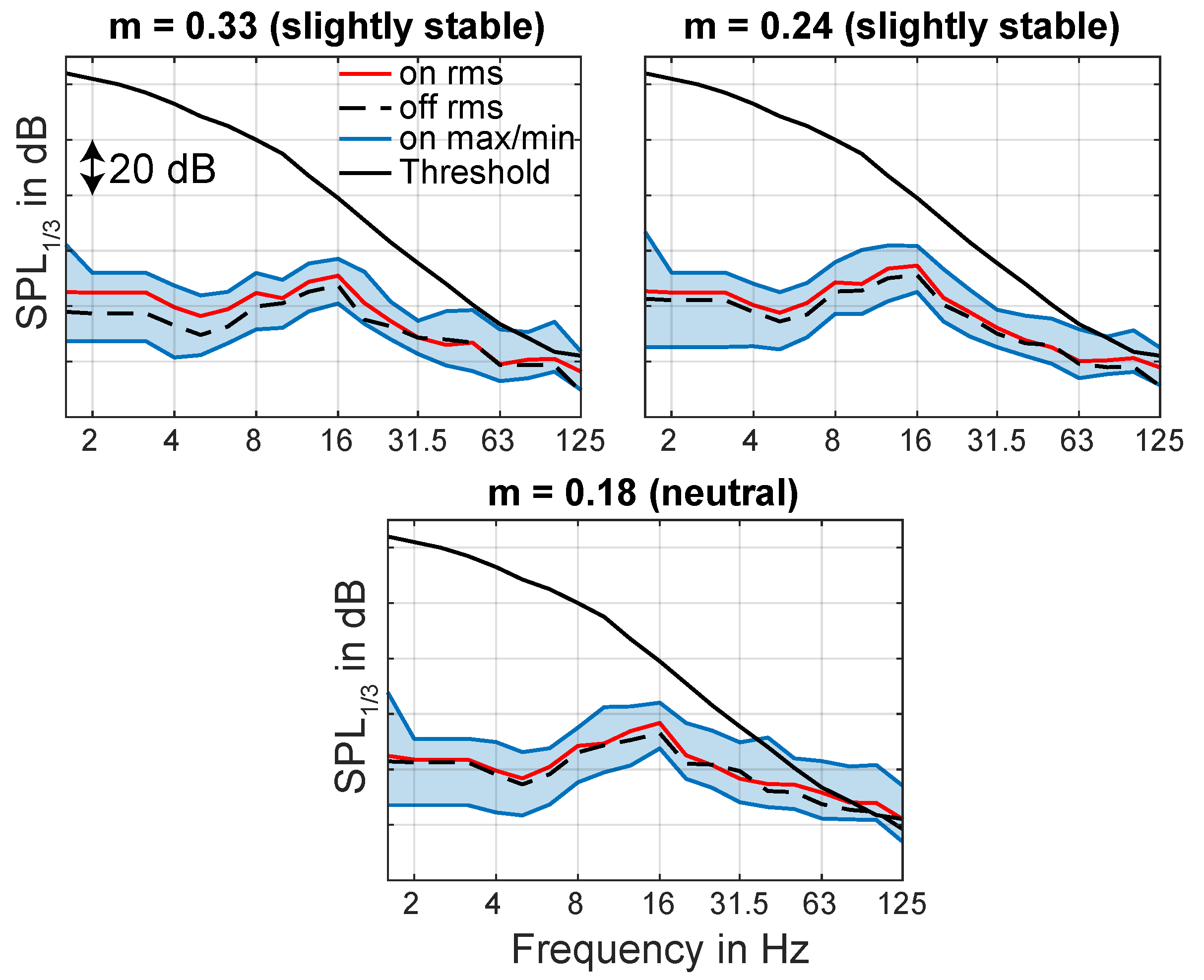
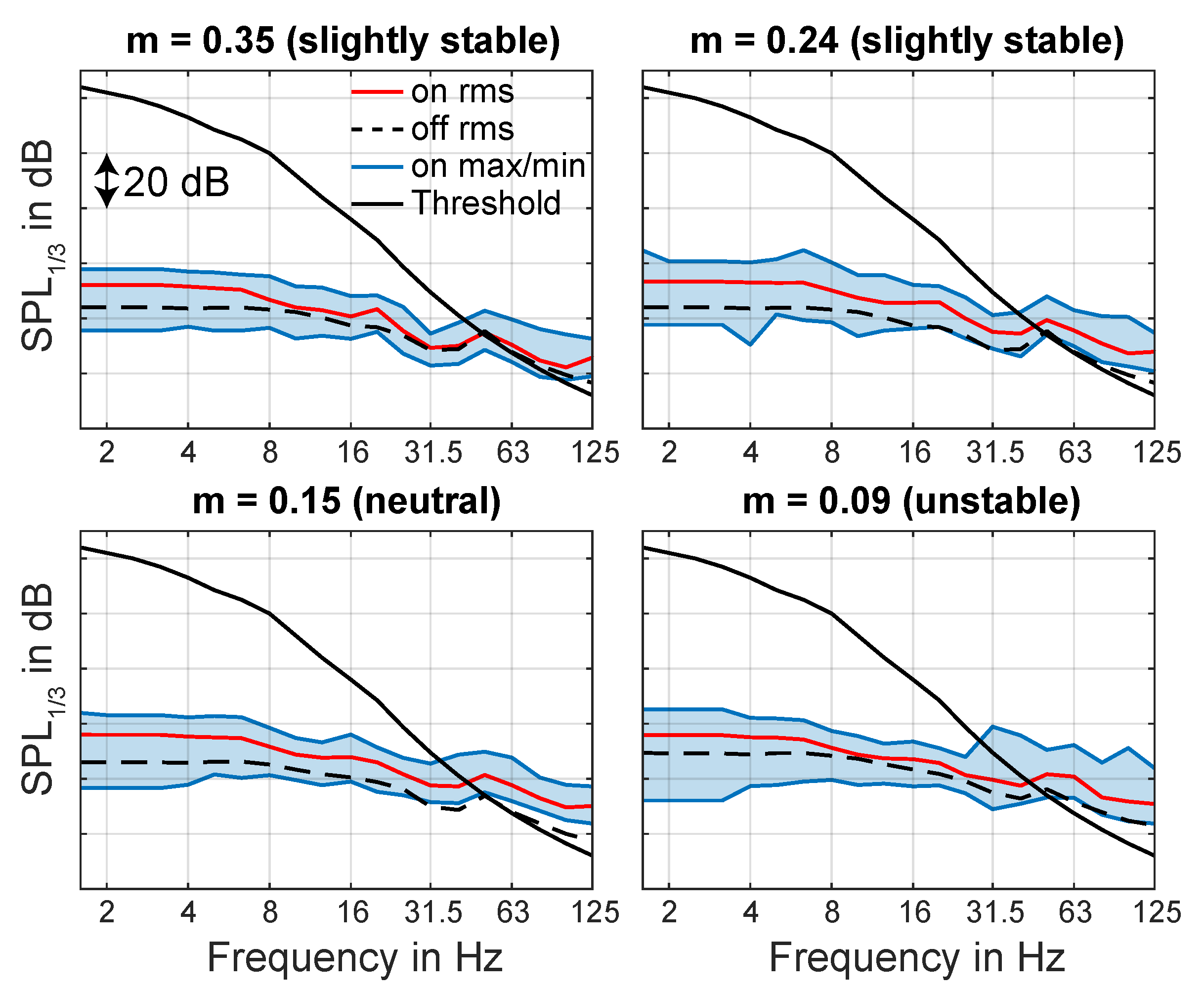
Figure 23 shows the unweighted on/off one-third octave spectra measured inside at location L3 for the described time periods in
Table 5 compared with the human hearing threshold. It can be seen that infrasonic sound is below the hearing threshold. For slightly stable conditions (
m = 0.35), the WT rms sound spectrum with rotating WT exceeded the threshold above 50 Hz. For slightly stable (
m = 0.24), neutral, and instable conditions, the threshold exceeded 40 Hz. The influence of atmospheric conditions was less obvious when plotting one-third octave spectra compared to the narrow-band-spectra in
Figure 19.
As already described by [
13], the large variation of maximum and minimum SPL for each considered 10 min period spectrum could lead to a better perception by residents or even annoyance. It was also confirmed by [
27] that with increasing amplitude-modulation depth, which could be related to the high variation of SPL, the annoyance of residents increased. However, it was also stated that low frequency components were not the main factors of annoyance. In this case, it also has to be noted that the measurements at Site 1 were conducted inside of a wooden shelter with clearly less damping effect on incoming acoustic waves compared to ordinary massive buildings and windows.
For comparison, unweighted one-third octave spectra for three different atmospheric conditions with the same rotational speed for Site 2 and measurement location L6 are shown in
Figure 24. The 10 min time periods where chosen to match the previous conditions in
Figure 23. Detailed information for each time period is given in
Table 7.
For slightly stable conditions, the WT rms sound spectrum with rotating WT exceeded the threshold above 125 Hz, and for neutral conditions, the threshold exceeded 63 Hz. The higher distance between the closest WT (WT8; see
Figure 1) of about 1450 m was clearly visible due to lower SPL, although L6 was located beside a wind farm. A peak in the 16 Hz third octave band not related to the WT as also occurring during shutdown was also observed in [
3] and related to a resonance of the building structure. The peak was much more dominant on Site 2 than Site 1, which could be explained by the masonry construction of the building in L6 compared to the single-wall construction of Location L3 and therefore different structural resonances.
To which extent the acoustic signals of the WT contributed to annoyance needs further investigation.
4.6. Limitations of the Study
Measurements of low frequency acoustic noise emitted by WT in populated areas are a challenging task. The presented results of this study were therefore limited in various ways. For example, the results of measurements inside could differ depending on the floor level, room dimensions, and mostly because of anthropogenic noise besides wind turbines. This led to the limitation that almost exclusively time periods during the night were evaluated, although the intensity of low frequency noise could be higher during the day.
A further limitation was that only one microphone could be placed near the WT and two microphones inside of buildings at the same time. As a consequence, the propagation of acoustic waves in different directions (directivity) could not be investigated. Furthermore, the decay of acoustic signals with distance was not evaluated in detail because more measurement locations, respectively infrasound microphones, would be necessary.
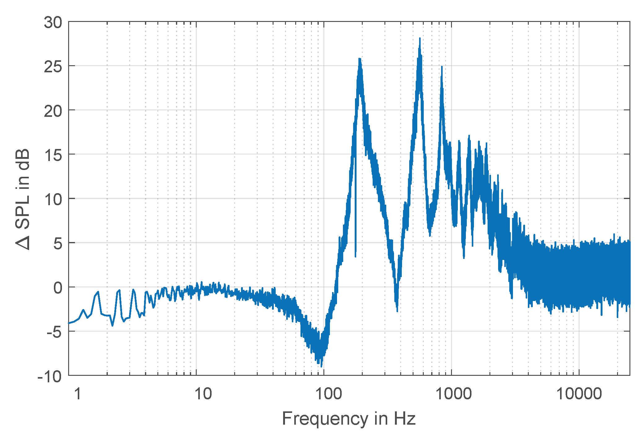
One key factor for reliable results is the measuring equipment itself. The measurement of sound pressure for frequencies below 20 Hz is strongly influenced by the cartridge thermal noise of the microphone capsule, the
-noise of the microphone preamplifier with corner frequencies around 10 to 20 Hz, and the
-noise of the recording systems. The noise of a microphone preamplifier is dominant for systems without weighting filters (e.g., A-weighting). Tests under acoustic low noise conditions in the laboratory by night have been carried out to get a better insight into this topic. For the noise test of the recording system, the input was connected to a resistive load with the value of the output impedance of the microphone. The noise spectra of the recording system within 0.1 Hz to 50 Hz itself were more than 30 dB lower compared to the spectra including the microphone. Robust capsules with a 1 inch, or better 2 inch, diameter and therefore higher sensitivity for field measurements are a better choice for infrasound applications, but they were not available on the market for ordinary users at the time of this project. Nevertheless, the comparison of spectra in
Figure 19 for non-operating and operating WT showed that the first BPF of around 0.8 Hz was well detectable. This was only possible if the measured values lied significantly above the noise of the microphone, especially the
-noise of the microphone preamplifier.


