Liver Backscatter and the Hepatic Vasculature’s Autocorrelation Function


1
Department of Physics and Astronomy, University of Rochester, Rochester, NY 14627, USA
2
Department of Medicine, University of Rochester Medical Center, Rochester, NY 14623, USA
3
Department of Electrical and Computer Engineering, University of Rochester, Rochester, NY 14627, USA
*
Author to whom correspondence should be addressed.
Acoustics 2020, 2(1), 3-12; https://doi.org/10.3390/acoustics2010002
Submission received: 5 December 2019
/
Revised: 9 January 2020
/
Accepted: 17 January 2020
/
Published: 22 January 2020
Abstract
:Ultrasound imaging of the liver is an everyday, worldwide clinical tool. The echoes are produced by inhomogeneities within the interrogated tissue, but what are the mathematical properties of these scatterers? In theory, the spatial correlation function and the backscatter coefficient are linked by a Fourier transform relationship, however direct measures of these are relatively rare. Under the hypothesis that the fractal branching vasculature and fluid channels are the predominant source of scattering in normal tissues, we compare theory and experimental measures of the autocorrelation function, the frequency dependence of scattering, and fractal dimension estimates from high contrast 3D micro-CT data sets of rat livers. The results demonstrate a fractal dimension of approximately 2.2 with corresponding power law estimates of autocorrelation and ultrasound scattering. These results support a general framework for the analysis of ultrasound scattering from soft tissues.
1. Introduction
In the long history of research on waves, the propagation of light or sound through a weakly inhomogeneous medium has been shown to be related to the spatial correlation function, a statistical measure of the material’s fluctuations in properties such as density or index of refraction [1,2]. Fluctuations in the forward propagating wave and the creation of scattered waves from the inhomogeneities have theoretical links to the spatial distribution of material properties. Important formulations of weak scattering known as the Born approximation have produced a simple integral relation between the averaged scattered intensity as a function of frequency, and the spatial correlation function of the inhomogeneous material. These statistical or ensemble average measures are related by a 3D Fourier transform relation [1,2], and so knowledge of the scattering structures within tissues and organs, and their shapes and statistical properties, is key to understanding the scattered waves or echoes in ultrasound imaging. Recently, we proposed that the branching vasculature and fluid-filled channels within soft tissues, modeled as fractal branching structures, play a dominant role in producing echoes [3], thus the spatial autocorrelation function is a key measure for predicting or analyzing waveforms. Unfortunately, there are a paucity of experimental results in the literature that directly address the fundamental issue of the 3D autocorrelation function of vascular shapes responsible for scattering in tissue.
The issue is relevant and significant because the 3D spatial autocorrelation function of these scattering sites determines the behavior of wave propagation, influencing the appearance of the uncountable numbers of ultrasound images that are taken every day for diagnostic purposes. To address this need, we have utilized X-ray contrast agent enhanced micro-CT images of the hepatic vasculature of rats. By thresholding the 3D volumetric image to isolate the contrast-filled vessels, spatial correlation functions of the branching structures can be calculated. The results are compared with analytical power law models associated with fractal structures, and they provide a necessary foundation for the theoretical prediction of wave propagation within and scattering from the normal liver.
While the concept of fractals [4] in biological systems has seen numerous applications [5,6], the nature of scattering from fractal structures has seen limited attention. Various predictions for scattering were made by Lin et al. [7] modeling fractal aggregates, Javanaud [8], and Shapiro [9]. Sheppard, and Connolly [10] considered the optical scattering from random surfaces. Shear wave scattering and loss were attributed to fractal structures in Lambert et al. [11] and Posnansky et al. [12]. The interrelationship of these different results and their application in the ultrasound examination of soft tissues requires further study.
In short, there have been a number of theoretical functions proposed for random media that are related to fractal models and which are linked to a variety of power law metrics. Yet these leave some open questions as to the particular autocorrelation function found in practice, and its implications for wave propagation and scattering. These are addressed in the following sections, first with the review of the relevant scattering theory and then experimental results from the hepatic vasculature.
2. Theory of Scattering Applied to Fractal Branching Networks
2.1. General Theory
In the theories of weak scattering from random media, it has been shown [13,14,15] that the differential scattering cross section per unit volume and the spatial correlation function of the inhomogeneities are related by
where is the wavenumber, is the vector separation between two points within the ensemble average, and is a constant. Assuming the correlation function is isotropic and simply dependent on separation distance , the volume integral reduces to
similar to the integral found in Equations (4), (9), and (11) from Parker [16] covering both acoustic and electromagnetic scattering under the Born approximation.
Significantly, Equations (1) and (2) conform the 3D Fourier transform in spherical coordinates with spherical symmetry, denoted as [17,18], and shown as follows using Bracewell’s convention
Thus, for isotropic 3D distributions, Equation (1) can be written as
Equation (4) demonstrates the important interpretation of scattering as a 3D spatial Fourier transform of the correlation function, assumed to be isotropic in this case. Thus, it is necessary to determine the spatial correlation function of the branching vasculature, beginning with a canonical cylindrical element, and this is determined in the next section.
2.2. The Long Vessel
We represent a long vascular channel as a cylinder of radius a,
where κ0 is the fractional variation in density plus incompressibility, assumed to be consistent with the Born formulation, F(ρ) represents the Hankel Transform, which is the 2 dimensional Fourier transform of a radially symmetric function, and ρ is the spatial frequency [17,19].
Assuming the fluid-filled cylinder is long in the -axis, then the shape is one-dimensional and its autocorrelation can be obtained from the inverse Hankel transform of the square of the shape’s Hankel transform
where ρ is the spatial frequency. Furthermore, we assume that cylinders of this kind exist within a fractal geometry in an isotropic pattern. Therefore, copies of this are interrogated by the forward wave over all possible angles. Thus, we find that [3] the spherically symmetric, isotropic transform Bs(q) is given by
Equation (7) represents the ensemble average 3D transform of an isotropic set of cylinders of some radius. However, we must also consider the cross-correlation of an ensemble of these elements and all other (including larger and smaller) elements within a fractal structure needs to be derived. The simplest assumption is that each generation of cylinders has an autocorrelation function with itself that has been determined (above), and that within the ensemble average the cross terms with all other branches (larger and smaller within the fractal structure) is simply a small constant that is nearly invariant with position and therefore can be neglected except for spatial frequencies nearing zero. Under that very simplistic assumption, the overall autocorrelation function is given by the sum (or integral in the continuous limit) of the different sizes’ correlation functions over all generations of branches, weighted by their relative numbers (number density in the continuous limit). Fractal structures in 3D and volume filling in 3D may be characterized by number density functions N(a) that are represented by N0/ab, where a is the characteristic radius of the canonical element, N0 is a global constant, and b is the power law coefficient [20].
Averaging over all sizes, in the 3D transform domain
and for our specific model, this becomes
where is a function of and with reference to Equation (4), we find that the predicted backscatter is
Also, the autocorrelation function is found from the inverse Fourier transform of Equation (9) to be and where for the convergence of the inverse transform integral, , and where is a constant. Thus, for example, if an eigenfunction of the transform occurs:
To combine these key relationships and restate them in terms of the fractal dimension D, Table 1 provides a summary of the theories.
3. Methods
3.1. Experimental Animals
The Institutional Animal Care and Use Committee at the University of Rochester approved all studies before initiation. For this preliminary study, two 8-week-old female Sprague-Dawley rats (Charles River Laboratories, Wilmington, MA, USA) that weighed ~200 g were given food (standard rodent diet provided by the University of Rochester Vivarium) and water ad libitum before randomization. The animals were maintained on a 12-h light-dark cycle in a controlled temperature of 74 °F with humidity of 37%.
3.2. Micro-CT
At euthanization, the hepatic artery was isolated and the inferior vena cava nicked as an egress; livers were perfused first with heparinized saline and then a warm (39–41°C) solution of 30% barium (Liquid E-Z-Paque, E-Z-EM, Inc., Lake Success, NY, USA) suspended in 1% agarose (Fisher Scientific, Fair Lawn, NJ, USA). The liver was immediately iced to set the agarose and then fixed with a mixture of methanol 60% (Fisher Scientific)/acetic acid 10% (Macron Chemicals, Center Valley, PA, USA)/water 30%. We imaged the right major lobe on a Bruker Skyscan (Kontich, Belgium) 1174 system with a 16.5 voxel size and the following imaging conditions: 50 kVp; 800 uA; 1,600-ms exposure; rotation step: 0.50°; and frame averaging: 2. The liver volume was reconstructed from the raw files using NRECON (Skyscan Bruker) with a 20% beam hardening correction value, ring artifact correction 10, and cone-beam reconstruction mode. The image processing was simplified by the high contrast between the vascular branches and tissue. Simple thresholding was used to isolate the branching vasculature within the 3D CT volume. The question of optimal threshold was addressed in two ways. First, a graph of the total number of connected branches above threshold was constructed as a function of increasing threshold value. Above a threshold of approximately 80 (out of 256 maximum value), the number of connected branches began to decrease sharply. Therefore, this suggested an optimal threshold below 80. Secondly, visual inspection of the thresholded 3D data sets was done to examine the presence or absence of broken branches or missing fine scale branches when the threshold is set too high. Regional merging of fine branch elements is seen when the threshold is set too low. These examinations suggested that the range of 60 to 80 was optimal for isolation of the branching vasculature for further analysis.
4. Results
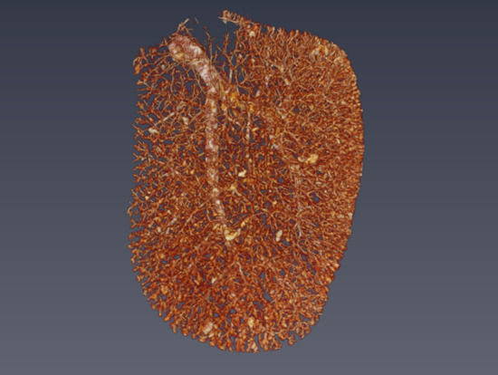
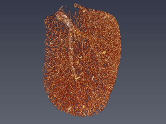
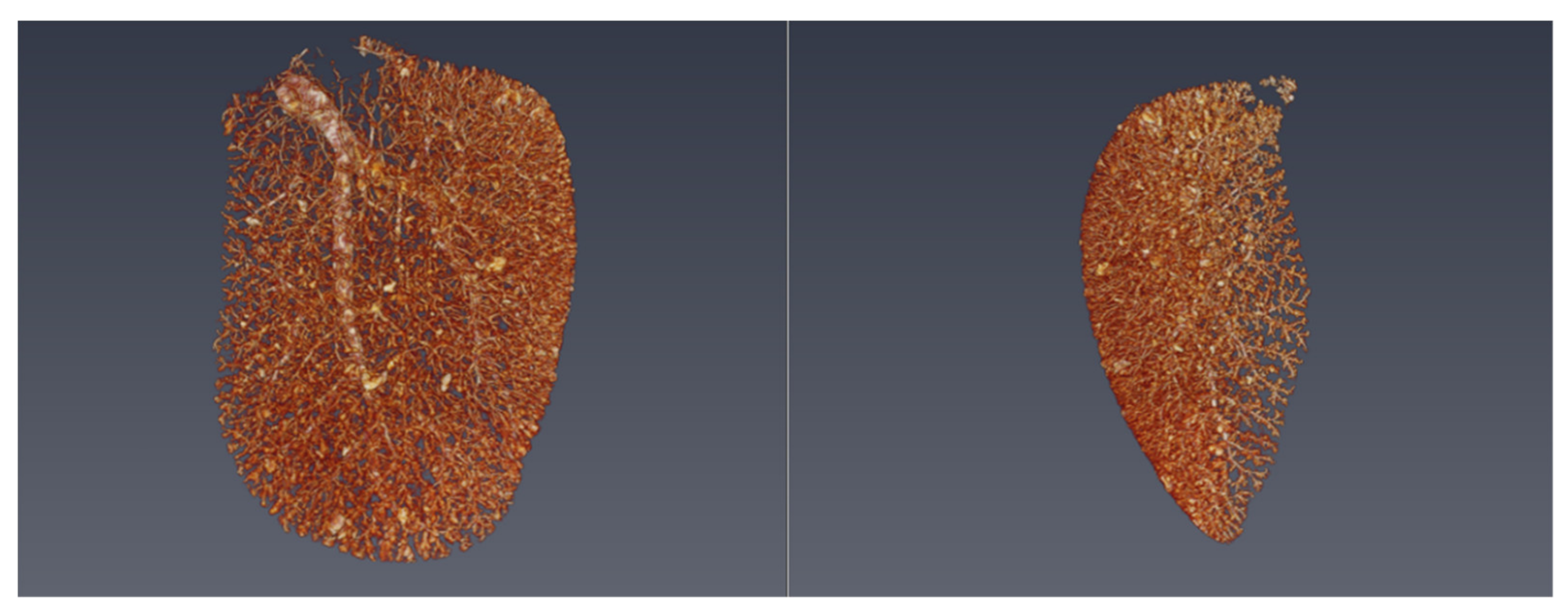
Examples of one liver CT volume after thresholding are shown in two rotations in Figure 1. Once the threshold was selected, the autocorrelation kernels were formed from internal cubes 30 voxels on each side, and located more than 30 voxels from the outer boundary of the perfused regions.
At that stage, each candidate autocorrelation volume kernel was sorted according to the number of voxels, N, that were occupied by a vessel, as described in Table 2. The reason for this sorting is that an autocorrelation window centered in the middle of the largest arterial branches has a maximum N and may show no decorrelation over significant lags. An opposite scenario is when an autocorrelation window contains only a few isolated voxels above threshold, in that case the result can also be spurious. This is related to the problem of limited scales of the fractal structure and a single scale of the autocorrelation calculation.
The different examples in Figure 2 and Figure 3 are illustrative of the range of different parameters. Nonetheless, an intermediate set of branching structures exist where the autocorrelation window may contain or interact with branches of various dimensions. These are depicted in Figure 2, where the top row indicates individual autocorrelation results and the bottom row the visual appearance of autocorrelation kernels, where N is above 100 and below 10,000. The power law fits to the autocorrelation functions in log-log space are given in Table 2 for different ranges of the voxel contents N, and fall in a range of approximately −0.8 to −1.2.
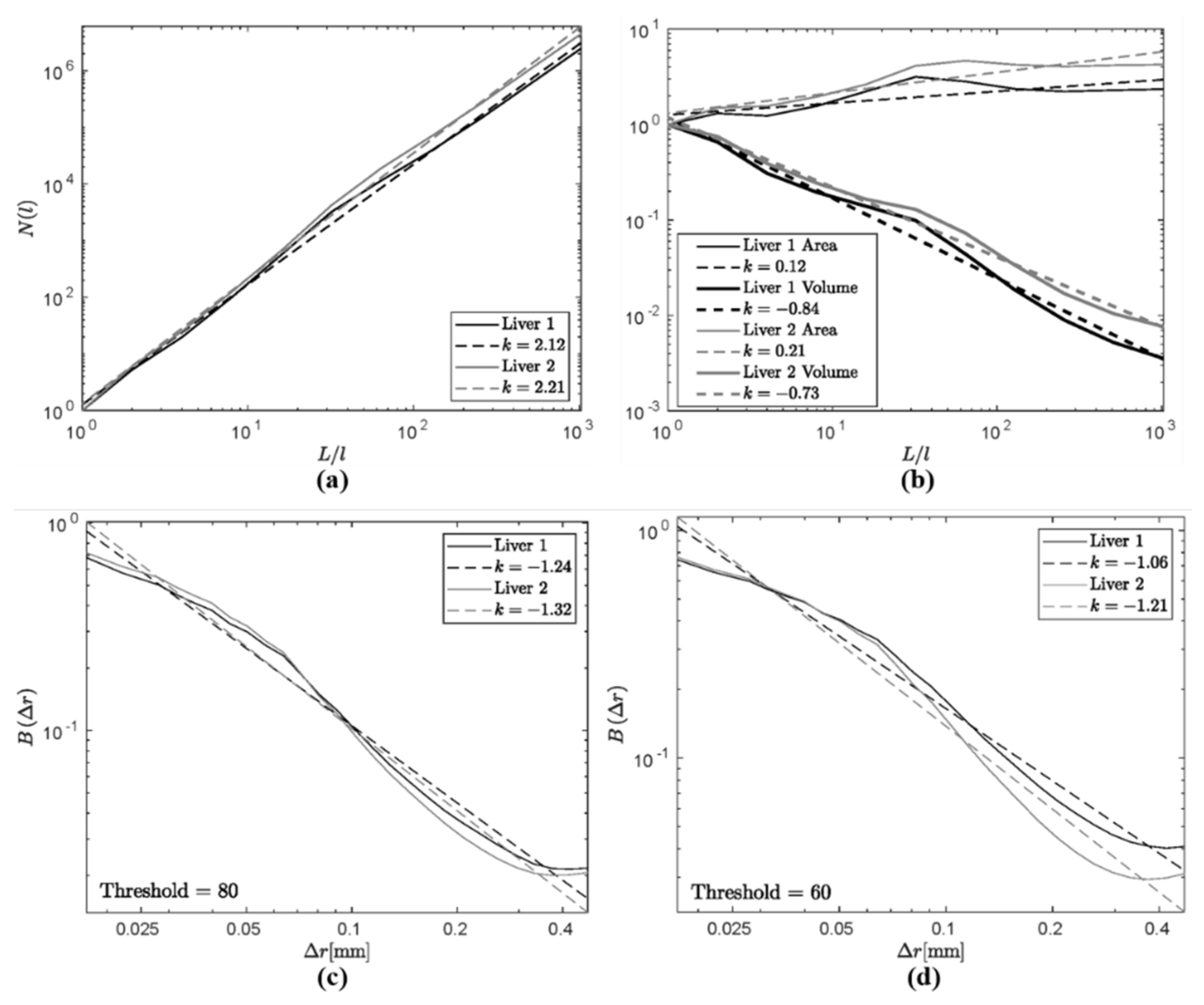
Switching to conventional metrics related to fractal dimension, Figure 3 provides the measures of box counting in 3a, the number of boxes needed to enclose the fractal structure as a function of scale, and box surface in 3b, along with selected ensemble autocorrelation plots in 3c and 3d, along with their respective power law fits.
These results are consistent with estimates of fractal dimension D around 2.2, and the different estimates are summarized in Table 3.
5. Discussion
5.1. Comparison of Measures
The spatial distribution of the vasculature has been assessed using different methods that are related to each other as summarized in Table 1 and in Chapters 1 and 2 of Vicsek [21]. These results show a range of estimated D as summarized in Table 3.
Variations in estimates occur naturally due to the inherent difficulty of measuring a multiscale structure with a single resolution metric (3D autocorrelations) and, furthermore, given the natural limits on largest and smallest structures available within the micro-CT volume rendering. These limitations are discussed in Viscek Chapter 4 [21]. In total, the estimates of D cluster around a value of 2.2, which coincided with the theoretical range (D < 3 for a 3D fractal structure) and with other results found in the literature for 3D pulmonary and placenta structures [20,22].
We note that the autocorrelation measures shown in Figure 2c and d could also suggest a decreased autocorrelation slope at small lags (below 0.06 mm) and a slightly higher slope at higher radial lags. This could be an artifact related to the difficulty in producing a low noise, high resolution vascular cast down to the smallest terminal branches, or alternatively could be an indication of a more complicated multi-fractal. This question will require further study. Another limitation of this study is the use of the hepatic artery as the contrast-enhanced vasculature. The liver also includes the hepatic vein and portal vein in its circulation [23], and these were not included in our 3D analysis. However, since these all have a connection within the fine grain hepatic sinusoidal system, it is plausible that the fractal dimension of these three systems is similar.
5.2. Implications for Scattering from Liver
Given a fractal dimension of approximately 2.2, the derivations in the Theory section and Table 1 would predict a backscatter coefficient from these livers that increases as roughly frequency to the 1.8 power, at least for wavenumbers commensurate with the scale of the branches and measurements, principally above 12 microns and below 100 microns. These scales would be commensurate with the frequencies and wavenumbers found in advanced animal imaging ultrasound systems that operate well above frequencies for human studies. Experimentally, most of the pioneering work on scattering in liver was done below 10 MHz. These early studies [24,25,26,27,28,29] demonstrated an increasing backscatter coefficient with increasing frequency. In particular, Campbell and Waag [24] reported a power law behavior in the 3–7 MHz band which is common to human abdominal scans, and found a power law coefficient of 1.4. This value is close to our estimate of 1.8 shown in Table 3, albeit for a smaller species and at resolutions that are relevant to higher frequencies than those employed in Waag’s studies. Later studies confirmed the trend of increasing backscatter with frequency extending up to 25 MHz [30,31,32,33].
Although our resolution is limited by the CT system and contrast enhancement, optical studies can obtain finer resolution. Schmitt and Kumar [34] studied phase contrast images of mouse liver histology slides and found a power law power spectrum behavior for spatial frequencies down to at least 1/10 microns.
Similarly, Rouyer et al. [33] studied thyroid tissue using broadband ultrasound systems and by replotting their data we can infer a power law behavior between 6 and 15 MHz, corresponding to wavelengths down to 100 microns.
5.3. Resolving Uncertainties and Future Work
In order to confirm these findings and theories at scales relevant to human examinations, two fronts need to be addressed. First, the ensemble average backscatter coefficient vs. frequency for adult normal human livers (and other soft tissues) must be assessed in the range of 2–15 MHz. Secondly, 3D vascularity measures of normal adult human tissues must be obtained at the highest possible resolution. The literature reports for human and bovine liver scattering are reasonably consistent with our results as they predict a power law increase in scattering with increasing frequency. Carefully calibrated measurements by Campbell and Waag [24] demonstrated a backscatter power law coefficient of approximately 1.4 in bovine liver at frequencies under 10 MHz commonly used in abdominal scanning of humans. Additional measurements in human livers, utilizing wide bandwidth systems and carefully imaged regions of interest within speckle regions are needed to better characterize the expected frequency dependence of backscatter from the normal liver.
In conjunction with this, high resolution 3D measurements of the vasculature within normal human livers are desired to test the direct link between the vasculature as primary scattering sites and the measured ultrasound backscatter. These contrast-enhanced vasculature studies at high resolution require special conditions. Only a few examples of high quality and high resolution 3D renderings of the branching vasculature have been reported for the brain [35] and the human placenta [36]. Given the few studies of this type reported in the literature, additional high resolution contrast vascular studies are warranted to define the normal range of parameters within Table 1 and Table 3. Ultimately, these should be measured for all soft tissues and organs that are routinely imaged using ultrasound pulse-echo techniques, including the prostate, thyroid, pancreas, liver, and brain.
6. Conclusions
High resolution contrast CT studies of a rat liver’s branching vasculature in 3D demonstrates a power law behavior for the 3D spatial autocorrelation function with an exponent between -0.8 and -1.2. This corresponds to a fractal dimension D in the range of 2.2 to 1.8. Box counting methods and related volume and surface metrics trend towards an estimate of D around 2.2. Correspondingly, a theoretical hypothesis about scattering from the fractal branching fluid-filled channels would result in the predicted backscatter vs. frequency having the form of a power law with dimension approaching 1.8. In other words, an f1.8 scattering relation will be observed within the scale of wavenumbers corresponding to the structure elements. This experimental result from spatial autocorrelation measurements is consistent with the general framework for fractal branching structures [21] and also with recent results determined in the human placenta [22]. It is an important first step to measure baseline parameter values in normal soft tissues. Once established, the important question of parameter sensitivity to pathologies will need careful examination, as subtle changes in tissue morphology then alter the backscatter and enable detection and staging of disease by ultrasound well before gross anatomical changes are imaged.
Author Contributions
Software and formal analysis, J.J.C.-N.; Theory and conceptualization, K.J.P.; Imaging methodology, R.W.W.; Micro-CT images, R.J.W. All authors have read and agreed to the published version of the manuscript.
Funding
This research was supported by the Hajim School of Engineering and Applied Sciences at the University of Rochester, and by the National Institutes of Health grant number R21EB025290.
Acknowledgments
The authors thank the Center for Integrated Research Computing (CIRC) at the University of Rochester for providing computational resources and technical support. The authors also thank Deborah Haight for imaging the liver on micro-CT.
Conflicts of Interest
The authors declare no conflict of interest.
References
- Debye, P.; Bueche, A.M. Scattering by an inhomogeneous solid. J. Appl. Phys. 1949, 20, 518–525. [Google Scholar] [CrossRef]
- Morse, P.M.; Ingard, K.U. Theoretical Acoustics; Chapter 8; Princeton University Press: Princeton, NJ, USA, 1987. [Google Scholar]
- Parker, K.J. Shapes and distributions of soft tissue scatterers. Phys. Med. Biol. 2019, 64, 175022. [Google Scholar] [CrossRef]
- Mandelbrot, B.B. Fractals: Form, Chance, and Dimension; W.H. Freeman: San Francisco, CA, USA, 1977; pp. 1–365. [Google Scholar]
- Bassingthwaighte, J.B.; Bever, R.P. Fractal correlation in heterogeneous systems. Physica D 1991, 53, 71–84. [Google Scholar] [CrossRef]
- Glenny, R.W.; Robertson, H.T.; Yamashiro, S.; Bassingthwaighte, J.B. Applications of fractal analysis to physiology. J. Appl. Physiol. 1991, 70, 2351–2367. [Google Scholar] [CrossRef] [PubMed] [Green Version]
- Lin, M.Y.; Lindsay, H.M.; Weitz, D.A.; Ball, R.C.; Klein, R. Universality of fractal aggregates as probed by light scattering. Proc. R. Soc. Lond. A Math. Phys. Sci. 1989, 423, 71–87. [Google Scholar]
- Javanaud, C. The application of a fractal model to the scattering of ultrasound in biological media. J. Acoust. Soc. Am. 1989, 86, 493–496. [Google Scholar] [CrossRef]
- Shapiro, S.A. Elastic waves scattering and radiation by fractal inhomogeneity of a medium. Geophys. J. Int. 1992, 110, 591–600. [Google Scholar] [CrossRef]
- Sheppard, C.J.R.; Connolly, T.J. Imaging of random surfaces. J. Mod. Opt. 1995, 42, 861–881. [Google Scholar] [CrossRef]
- Lambert, S.A.; Nasholm, S.P.; Nordsletten, D.; Michler, C.; Juge, L.; Sinkus, R.; Serfaty, J.M. Bridging three orders of magnitude: Multiple scattered waves sense fractal microscopic structures via dispersion. Phys. Rev. Lett. 2015, 115, 094301. [Google Scholar] [CrossRef] [PubMed] [Green Version]
- Posnansky, O.; Guo, J.; Hirsch, S.; Papazoglou, S.; Braun, J.; Sack, I. Fractal network dimension and viscoelastic powerlaw behavior: I. A modeling approach based on a coarse-graining procedure combined with shear oscillatory rheometry. Phys. Med. Biol. 2012, 57, 4023–4040. [Google Scholar] [CrossRef] [Green Version]
- Insana, M.F.; Wagner, R.F.; Brown, D.G.; Hall, T.J. Describing small-scale structure in random media using pulse-echo ultrasound. J. Acoust. Soc. Am. 1990, 87, 179–192. [Google Scholar] [CrossRef] [PubMed]
- Ishimaru, A. Wave Propagation and Scattering in Random Media; Academic Press: New York, NY, USA, 1978; Volume 2, pp. 1–572. [Google Scholar]
- Campbell, J.A.; Waag, R.C. Ultrasonic scattering properties of three random media with implications for tissue characterization. J. Acoust. Soc. Am. 1984, 75, 1879–1886. [Google Scholar] [CrossRef] [PubMed]
- Parker, K.J. Hermite scatterers in an ultraviolet sky. Phys. Lett. A 2017, 381, 3845–3848. [Google Scholar] [CrossRef]
- Bracewell, R.N. The Fourier Transform and its Applications; Chapter 12; McGraw-Hill: New York, NY, USA, 1965. [Google Scholar]
- Baddour, N. Operational and convolution properties of three-dimensional Fourier transforms in spherical polar coordinates. J. Opt. Soc. Am. A Opt. Image Sci. Vis. 2010, 27, 2144–2155. [Google Scholar] [CrossRef] [PubMed]
- Erdélyi, A.; Bateman, H. Tables of Integral Transforms; McGraw-Hill: New York, NY, USA, 1954; Volume 2. [Google Scholar]
- Krenz, G.S.; Linehan, J.H.; Dawson, C.A. A fractal continuum model of the pulmonary arterial tree. J. Appl. Physiol. 1992, 72, 2225–2237. [Google Scholar] [CrossRef]
- Vicsek, T. Fractal Growth Phenomena, 2nd ed.; World Scientific: Singapore, 1992. [Google Scholar]
- Parker, K.J.; Carroll-Nellenback, J.J.; Wood, R.W. The 3D spatial autocorrelation of the branching fractal vasculature. Acoustics 2019, 1, 20. [Google Scholar] [CrossRef] [Green Version]
- Guyton, A.C. Textbook of Medical Physiology, 4th ed.; Saunders: Philadelphia, PA, USA, 1971; pp. 1–1032. [Google Scholar]
- Campbell, J.A.; Waag, R.C. Measurements of calf liver ultrasonic differential and total scattering cross sections. J. Acoust. Soc. Am. 1984, 75, 603–611. [Google Scholar] [CrossRef]
- Bamber, J.C.; Hill, C.R. Acoustic properties of normal and cancerous human liver—I. Dependence on pathological condition. Ultrasound Med. Biol. 1981, 7, 121–133. [Google Scholar] [CrossRef]
- Nicholas, D. Evaluation of backscattering coefficients for excised human tissues: Results, interpretation and associated measurements. Ultrasound Med. Biol. 1982, 8, 17–28. [Google Scholar] [CrossRef]
- Lizzi, F.L.; Greenebaum, M.; Feleppa, E.J.; Elbaum, M.; Coleman, D.J. Theoretical framework for spectrum analysis in ultrasonic tissue characterization. J. Acoust. Soc. Am. 1983, 73, 1366–1373. [Google Scholar] [CrossRef]
- D’Astous, F.T.; Foster, F.S. Frequency dependence of ultrasound attenuation and backscatter in breast tissue. Ultrasound Med. Biol. 1986, 12, 795–808. [Google Scholar] [CrossRef]
- Reid, J.M.; Shung, K.K. Quantitative measurements of scattering of ultrasound by heart and liver. Ultrason. Tissue Charact. II 1979, 2, 153–156. [Google Scholar]
- Ghoshal, G.; Lavarello, R.J.; Kemmerer, J.P.; Miller, R.J.; Oelze, M.L. Ex Vivo study of quantitative ultrasound parameters in fatty rabbit livers. Ultrasound Med. Biol. 2012, 38, 2238–2248. [Google Scholar] [CrossRef] [Green Version]
- Lu, Z.F.; Zagzebski, J.A.; Lee, F.T. Ultrasound backscatter and attenuation in human liver with diffuse disease. Ultrasound Med. Biol. 1999, 25, 1047–1054. [Google Scholar] [CrossRef]
- Oelze, M.L.; Zachary, J.F. Examination of cancer in mouse models using high-frequency quantitative ultrasound. Ultrasound Med. Biol. 2006, 32, 1639–1648. [Google Scholar] [CrossRef] [PubMed]
- Rouyer, J.; Cueva, T.; Yamamoto, T.; Portal, A.; Lavarello, R.J. In Vivo estimation of attenuation and backscatter coefficients from human thyroids. IEEE Trans. Ultrason. Ferroelectr. Freq. Control 2016, 63, 1253–1261. [Google Scholar] [CrossRef]
- Schmitt, J.M.; Kumar, G. Turbulent nature of refractive-index variations in biological tissue. Opt. Lett. 1996, 21, 1310–1312. [Google Scholar] [CrossRef]
- Risser, L.; Plouraboue, F.; Steyer, A.; Cloetens, P.; le Duc, G.; Fonta, C. From homogeneous to fractal normal and tumorous microvascular networks in the brain. J. Cereb. Blood Flow Metab. 2007, 27, 293–303. [Google Scholar] [CrossRef]
- Parker, K.J.; Ormachea, J.; McAleavey, S.A.; Wood, R.W.; Carroll-Nellenback, J.J.; Miller, R.K. Shear wave dispersion behaviors of soft, vascularized tissues from the microchannel flow model. Phys. Med. Biol. 2016, 61, 4890. [Google Scholar] [CrossRef]
Figure 1.
Micro-CT volume rendering of the high contrast liver vasculature created by thresholding; two views corresponding to rotation of the 3D structure are shown. Voxel dimensions are 16.5 microns.
Figure 1.
Micro-CT volume rendering of the high contrast liver vasculature created by thresholding; two views corresponding to rotation of the 3D structure are shown. Voxel dimensions are 16.5 microns.

Figure 2.
The top row shows, for each region, the normalized autocorrelation for each displacement (dots) as well as the average overall vector displacements in 3D, for each radial bin for a range of N = B(0) (red line). The bottom row shows intensity projections for four sub-volumes of the 1000 autocorrelation windows, with their surrounding neighborhoods.
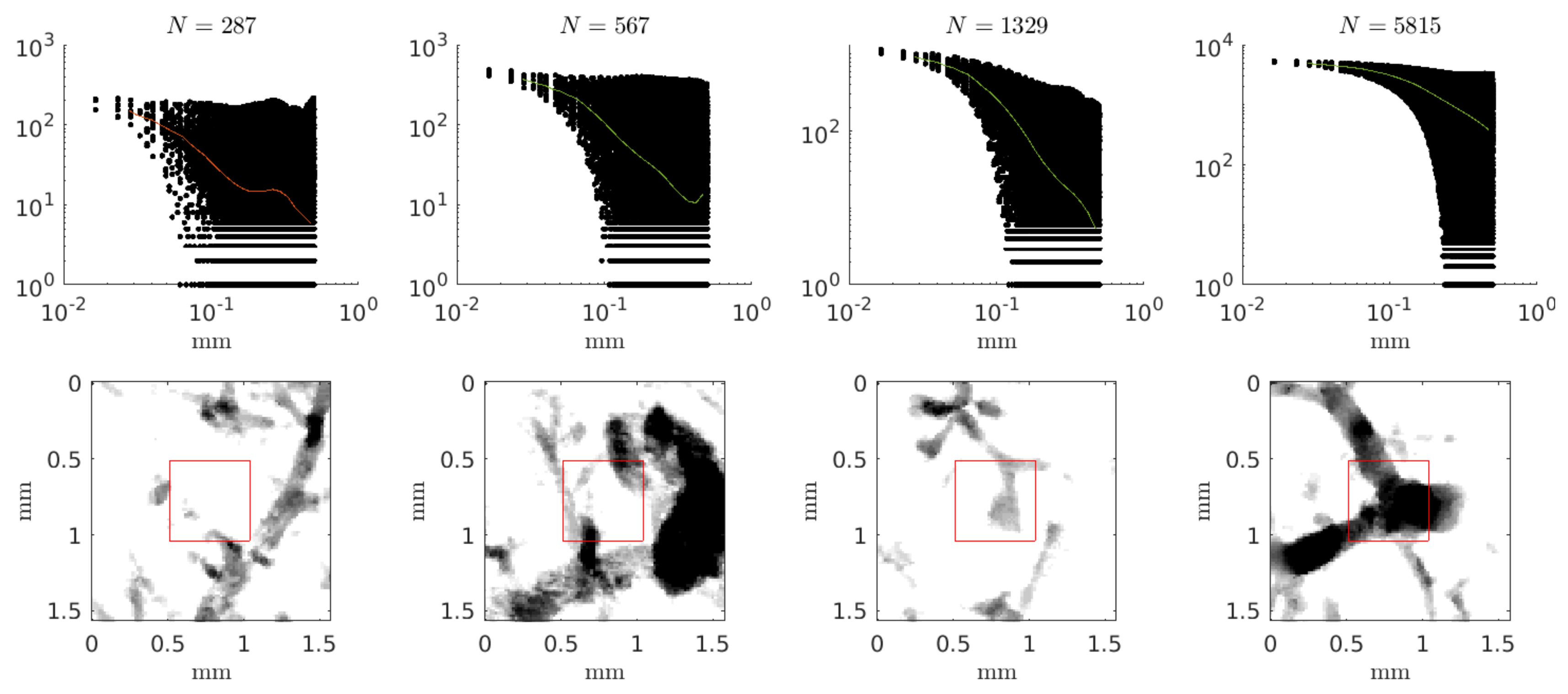
Figure 3.
(a) Plot showing the number of boxes N(l) that are required to enclose the fractal structure (threshold = 80) as a function of scale (L/l) on log-log plot. L is the largest length of the structure, 17 mm. (b) Plot similar to (a) showing the surface area and volume (threshold = 80) of the boxes that conform to the vasculature. (c) Plot showing the fit to the autocorrelation function for 10 < N < 1000 (threshold = 80). (d) Autocorrelation function for 10 < N <1000 for threshold = 60. Results from liver 1 and 2 are shown in each.


Table 1.
Interrelationship of fractal metrics in 3D.
| Name | Symbol | Equation | Notes |
|---|---|---|---|
| Fractal dimension | |||
| Autocorrelation | |||
| 3D spherical Fourier transform | |||
| Scattering differential cross section |
Table 2.
Power law fits to autocorrelation functions can vary with the threshold used to generate the binary vasculature structures, and the number of points N above threshold contained in the selected autocorrelation voxels.
Table 2.
Power law fits to autocorrelation functions can vary with the threshold used to generate the binary vasculature structures, and the number of points N above threshold contained in the selected autocorrelation voxels.
| Liver | Threshold | N, Lower Bound | N, Upper Bound | Power Law | Regions |
|---|---|---|---|---|---|
| 1 | 60 | 10 | 100 | −0.91 | 49 |
| 60 | 100 | 1000 | −1.09 | 172 | |
| 60 | 1000 | 10000 | −0.79 | 279 | |
| 80 | 10 | 100 | −1.28 | 104 | |
| 80 | 100 | 1000 | −1.23 | 210 | |
| 80 | 1000 | 10000 | −0.84 | 126 | |
| 2 | 60 | 10 | 100 | −1.16 | 50 |
| 60 | 100 | 1000 | −1.22 | 187 | |
| 60 | 1000 | 10000 | −0.87 | 253 | |
| 80 | 10 | 100 | −1.28 | 80 | |
| 80 | 100 | 1000 | −1.32 | 219 | |
| 80 | 1000 | 10000 | −0.87 | 137 |
Table 3.
Approximate values of D from different metrics. The estimated slope γ is from log-log plots of the metric vs. scale.
Table 3.
Approximate values of D from different metrics. The estimated slope γ is from log-log plots of the metric vs. scale.
| Method | Dependence | Estimates |
|---|---|---|
| Autocorrelation | D = 3 − γ | 2.2 > D > 1.8 |
| Surface area | D = 2 + γ | 2.1 |
| Volume | D = 3 + γ | 2.2 |
| Box counting | D = γ | 2.2 |
| Backscatter (predicted) | ∼k4−D | k1.8 |
© 2020 by the authors. Licensee MDPI, Basel, Switzerland. This article is an open access article distributed under the terms and conditions of the Creative Commons Attribution (CC BY) license (http://creativecommons.org/licenses/by/4.0/).
Share and Cite
MDPI and ACS Style
Carroll-Nellenback, J.J.; White, R.J.; Wood, R.W.; Parker, K.J. Liver Backscatter and the Hepatic Vasculature’s Autocorrelation Function. Acoustics 2020, 2, 3-12. https://doi.org/10.3390/acoustics2010002
AMA Style
Carroll-Nellenback JJ, White RJ, Wood RW, Parker KJ. Liver Backscatter and the Hepatic Vasculature’s Autocorrelation Function. Acoustics. 2020; 2(1):3-12. https://doi.org/10.3390/acoustics2010002
Chicago/Turabian StyleCarroll-Nellenback, Jonathan J., R. James White, Ronald W. Wood, and Kevin J. Parker. 2020. "Liver Backscatter and the Hepatic Vasculature’s Autocorrelation Function" Acoustics 2, no. 1: 3-12. https://doi.org/10.3390/acoustics2010002