Article

Effect of Tip Mass Length Ratio on Low Amplitude Galloping Piezoelectric Energy Harvesting

by
Mohammad Yaghoub Abdollahzadeh Jamalabadi
Department of Mechanical, Robotics and Energy Engineering, Dongguk University-Seoul, Seoul 04620, Korea
Acoustics 2019, 1(4), 763-793; https://doi.org/10.3390/acoustics1040045
Submission received: 21 August 2019 / Revised: 17 September 2019 / Accepted: 20 September 2019 / Published: 24 September 2019

Abstract

:
Galloping beams were exposed to the wind free stream and is used for sustainable wind-power harnessing. In this paper, the effect of tip mass on the performance of a galloping energy harvester is investigated by simple modeling of the system, which is useful for broad engineering applications of these systems. Here, the piezoelectric layer attached to a cantilever beam with a tip mass exposed to the wind free stream is used as an energy harvester. A fluid–solid interaction model is used to simulate the problem. The fluid–solid interaction model is composed of the experimental data for aerodynamic loads and one-dimensional structural model of piezoelectric and beam material with Euler–Bernoulli beam theory. The governing partial differential equations of the system are solved analytically by use of the approximation method. The resulting model is confirmed by preceding experimental results. The effects of the tip mass length ratio on the onset of galloping, the level of the produced voltage, and the harvested power are determined analytically. As shown by increase of the length of tip mass for the constant beam and piezoelectric length, the inertia of the system increases while the tip displacement and onset of galloping decrease.

Graphical Abstract

1. Introduction

The elasticity of piezoelectric materials makes them possible energy harvesting materials from environmental vibrations. A review of vibration-based micro-generator piezoelectric energy harvesters by Saadon and Sidek [1] showed the wide applicability of piezoelectric power harvesting devices. The piezoelectric material can convert large amounts of strain to electrical energy. Two modes are important in the mechanical energy conversion of piezoelectric materials. One mode is based on applying the external force parallel to the poling direction, and the second is perpendicular. As the perpendicular mode has the lower coupling coefficient, it is used mostly in engineering applications.
Saadon and Sidek performed a review of vibration-based micro-electro-mechanical systems (MEMS) piezoelectric energy harvesters [1]. To convert the environmental excitations to strain, usually the bimorph configuration is used. An experimental investigation of the bimorph cantilever model for piezoelectric energy harvesting from base excitations was done by Erturk and Inman [2]. Many environmental sources such as raindrop impacts [3], sea waves [4,5], and galloping [6,7,8,9] could be used as a vibrational source of this device. Nonlinear modeling and analysis of piezoelectric energy harvesting from transverse galloping [10,11] and its coupling with electric loads [12] are performed in various studies.
The efficiency and optimal design of piezoelectric energy harvesting induced by galloping phenomena are typically explored mathematically. Although the models of References [13,14] are more accurate than the original model of Reference [9], they achieve unrealistic results though their simulations were not validated by proper experimental results. The use of the experiment results of Reference [8] as a benchmark is not a proper choice as the effect of tip mass is negligible in that study. The models presented in References [9,13,14,15] caused a great error in the calculation of harvested power which could be misleading for young researchers in the design of energy harvesting devices by the aid of piezoelectric materials. Although Sirohi and Mahadik [9,16] showed that their results are in good agreement with their numerical calculations, it is suspicious that they reached identical analytical results with two different methods. They used the formula for vibrating base excitation which does not include the effect of tip mass inertia [16] and coupled formulation [9], but they reached the same analytical results. Based on the results of Reference [9,13,14], the order of magnitude of power estimated is watts while the author’s experience [17,18] and benchmark [8] show maximum attainable power in milliWatts. Also, the effect of tip mass is studied in References [19,20]. The cases studied in Reference [19,20] are related to the cases where the bluff body subjected to wind flows or acceleration is concentrated at tip mass, and thus, the effect of the mass moment of inertia on dynamic calculation and the length of tip mass on the applied force and momentum is negligible. The degree of freedom of movement of the cantilever beam in References [19,20,21,22,23,24,25,26,27,28,29,30,31,32,33,34,35,36,37,38,39] is in a way that it cannot sense the effect of distributed tip mass and that the concentrated mass can lead to a sufficient solution.
Modeling and experimental verification of proof mass effects on vibration energy harvester performance by Kim et al. [19] and a comparative study of tip cross sections for efficient galloping energy harvesting by Yang et al. [20] are about the geometrical optimization of the system. Parkinson et al. investigated the various aspects of flow-induced vibration such as the following: square-section cylinder [21], the combined effects of vortex-induced vibration and galloping [22,23,24], turbulence effects on galloping of bluff cylinders [25], wind-induced instability [26], aeroelastic instability [27,28,29], wake source model for bluff body potential flow [30], square prism [31], galloping response of towers [32], and combined effects of galloping and vortex resonance [33]. Since Den Hartog [34] presented the galloping criterion in transmission line vibration due to sleet, the aeroelastic galloping of prismatic bodies has been studied in many researches [35]. Recently, Jamalabadi and Kwak presented a dynamic model of a galloping structure equipped with piezoelectric wafers and energy harvesting [36]. Their model is used in broad engineering applications. Also, Abdelkefi et al. [37], Ewere and Wang [38], and Rostami and Fernandes modeled the effect of inertia and flap on autorotation applied for hydrokinetic energy harvesting [39]. Although their model is comprehensive, it fails to present a simple form to use as a rule of thumb by engineers.
This paper is about the mass and the effect of geometry (tip mass length ratio) of the mass, which can affect the applied force and momentum. To compare with the results of Reference [8], the D-shaped tip mass has been considered. Although one case cannot conclude the effect of tip mass, as there was no experimental data for other shapes in the literature, just the modified versions of the previous method are presented. Different shapes of tip mass could be discussed in future researches. The manuscript has followed several studies on galloping energy harvesting, in particular, the configuration which is similar to that presented in Reference [9]. In this paper, the problem is solved completely and is correctly addressed. Furthermore, the approximate solution method is used to give an explicit solution to the problem for engineers who do not prefer to involve the mathematical complexity of the common methods for partial differential equation (PDE) solutions.

2. Mathematical Modeling
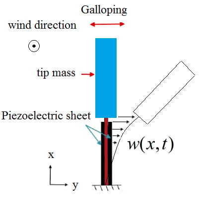
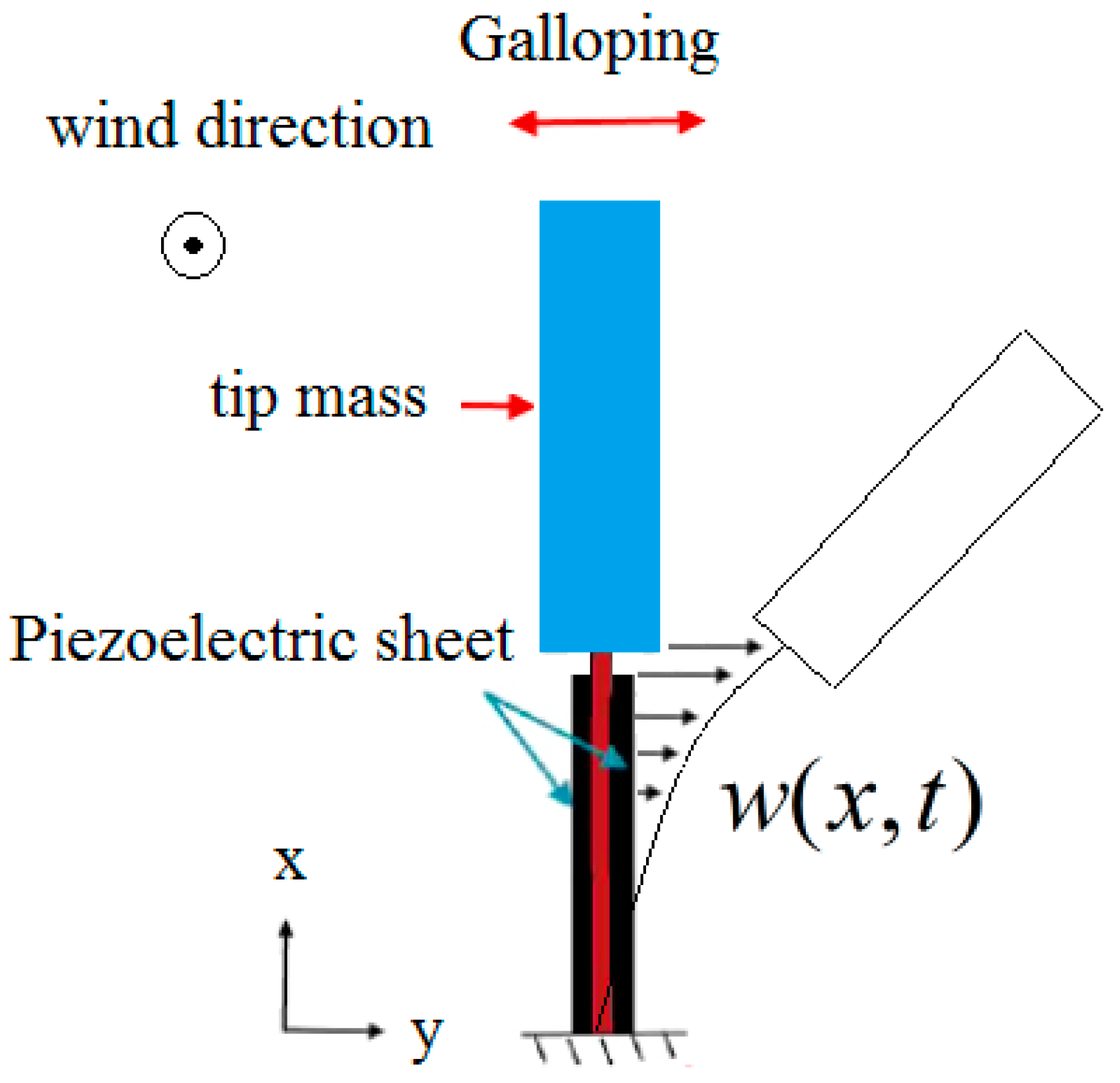
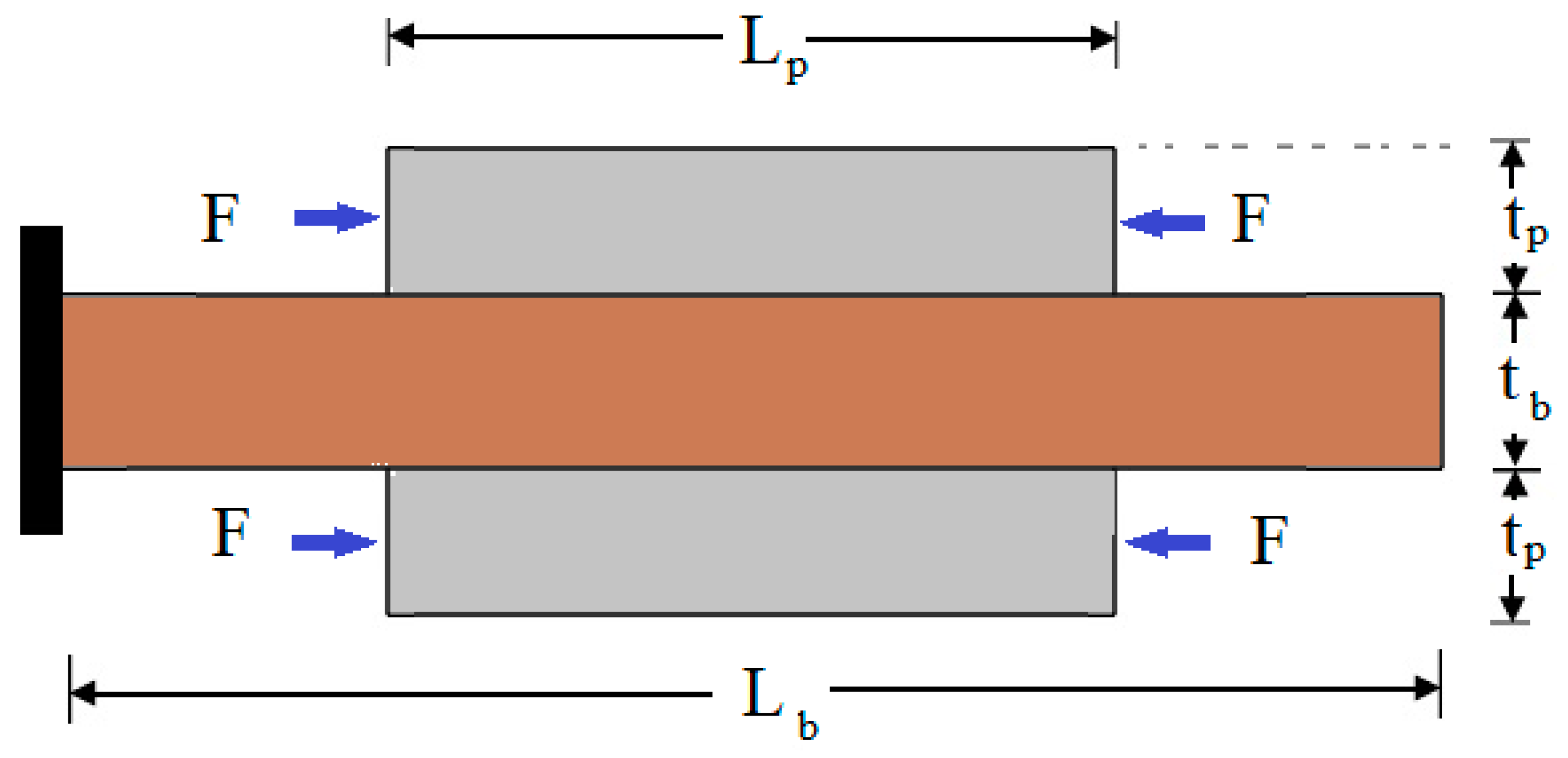
As presented in Figure 1, the system is composed of a cylinder tip mass (bluff body) mounted on an elastic beam made of aluminum and covered by two piezoelectric sheets (sheets are bonded on both sides) in an open environment with the wind velocity of V. The two piezoelectric plates plotted in Figure 1 are connected in parallel with opposite polarity to an electrical impedance R to harvest higher galloping energy. The free-body diagram of the tip mass which is exposed to an incoming flow in the z-direction with a magnitude of V is depicted in the top view of the problem for the D-shape cylindrical mass in Figure 2. The beam mounted bluff body experiences galloping in the x-y plane in the ±y direction when V is greater than the onset galloping velocity. The material properties of the system (cantilever beam, air, and the tip body) are presented in Table 1. As the system is exposed to the wind, it starts to vibrate (in the y-direction) to reach a stable oscillation. The strain produced in the base beam is converted to an electric charge in piezoelectric sheets.

2.1. Beam Modeling

The frequency of the vibration is equal to the fundamental mode of the beam (here, it is the bending mode and is a function of the Reynolds number as claimed in Reference [8]). The solid part of the system is modeled as follow:
The displacement of the beam is a function of time and is expressed using the modal expansion form (exact mode shapes of the structure):
w ( x , t ) = ϕ i ( x ) q i ( t )
where w(x,t) is the displacement of the beam; φi(t) is the ith mode shape; and qi(t) is the time-dependent part of the beam displacement, which is also mentioned in the literature as the mode coordinate. Each of the displacement functions is named a mode, and the shape of the displacement curve is named the mode shape. The Euler–Bernoulli beam model is composed of the second derivate of the internal moment; piezoelectric coupling term; and internal damping of the structure (strain rate), where the galloping aerodynamic moment and force are applied by the Dirac delta function at the end of the beam and the viscous air damping coefficient is neglected. The exact mode shapes of the structure are obtained by Euler–Bernoulli beam theory, including forcing, damping, and piezoelectric coupling terms:
ρ A 2 w t 2 + 2 x 2 I ( E 2 w x 2 + c 3 w x 2 t ) =   E p d 31 w p ( t p + t b ) [ d d x δ ( x x 1 ) ] x 1 = L 1 x 1 = L 2 V ( t ) + M t i p d d x δ ( x L ) + F t i p δ ( x L )
where E is Young′s modulus of material, I is the mass moment of inertia (calculated with respect to the axis perpendicular to the applied loading and passes through the centroid of the cross-section), c is the internal damping coefficient of structure (with the unit of kgm−1·s−1), ρ is the density of material, A is the cross-sectional area, Ep is the piezoelectric material’s Young′s modulus, d31 is the strain coefficient of piezoelectric, wp is the width of the piezoelectric layer, tp is the piezoelectric layer thickness, L1 and L2 are respectively the starting and ending points of the piezoelectric material sheets on the beam, δ is the delta Dirac function, V is the produced voltage at the electrodes, Mtip is the effective moment applied at the end of the beam by the tip mass, and Ftip is the effective force applied at the end of the beam by the tip mass. The left-hand side (LHS) of Equation (2) is the simplification of the time-dependent linear theory of elasticity, known as engineer′s beam theory (a special case of Timoshenko beam theory or classical beam theory), which offers a tool for calculating the small deflection characteristics of beams under lateral external loads. The first term in the LHS characterizes the inertial effect derived from kinetic energy while the second one in the LHS signifies the effective stiffness derived from potential energy due to internal forces. The right-hand side of Equation (2) has units of force per length composed of two sources of a distributed load of piezoelectric sheet and tip mass effect at the point of tip mass-beam connection. The piezoelectric load considered here is the ideal case which will be discussed more in Section 2.5, and the tip mass effects are retrieved from the first and second integrations of Equation (2) concerning the longitudinal direction which leads to shear force in the beam and to bending moment in the beam.
Estimate the exact mode shapes of the structure by dropping forcing, damping, and piezoelectric coupling terms from Euler–Bernoulli beam theory. As in the absence of a transverse load, the free vibration of the beam leads to the sum of harmonic vibrations (based on the Fourier decomposition); here, a sinusoidal form for the time-dependent part is assumed, and then, the resulting eigenvalue equation for the exact mode shapes of for each value of frequency of the beam is obtained by a partial differential equation:
2 x 2 ( E ( x ) I ( x ) 2 ϕ i ( x ) x 2 ) = ρ ( x ) A ( x ) ω i 2 ϕ i ( x )
where ωi is the natural frequency of the ith mode. The left-hand side of Equation (3) presents the second derivate of the bending moment with respect to the longitudinal position, while the right-hand side of Equation (3) presents the inertial terms. The Rayleigh method offers the same method for computation of the fundamental frequency of the system. As the displacement is not unique and depends on the frequency, the time-dependent part is given by the following:
q ¨ i ( t ) + 2 ξ ω q ˙ i ( t ) + ω 2 q i ( t ) =   [ ( ϕ i ( L p ) ϕ i ( 0 ) ) E p d 31 w p ( t p + t b ) ] V ( t ) +                     1 2 ρ a V D a 1 q ˙ i ( t ) [ ϕ i 2 ( L ) L r + ϕ i ( L ) ϕ i ( L ) L r 2 + ϕ i 2 ( L ) L r 3 ] +                     1 2 ρ a V 1 D a 3 q ˙ i 3 ( t ) [ ϕ i 4 ( L ) L r + 2 ϕ i 3 ( L ) ϕ i ( L ) L r 2 + 2 ϕ i 2 ( L ) ϕ i 2 ( L ) L r 3 + ϕ i 3 ( L ) ϕ i ( L ) L r 4 + ϕ i 4 ( L ) L r 5 5 ]
where ρa is the air density, Lr is the length of the tip body, D is the width of the tip body, V is the wind velocity, L is the length of the beam, tb is the beam material layer thickness, dot is used to present the derivative with respect to time, and prime is used for the first derivate versus location. The values of q (actually constants as there is one for each mode i), in general, are complex and are found by the initial conditions on the displacements and velocity of the beam. As the characteristic time scale of the flow motion is less than the characteristic time scale of the oscillations, the quasi-steady hypothesis is used to evaluate the galloping aerodynamic terms in the above equations.

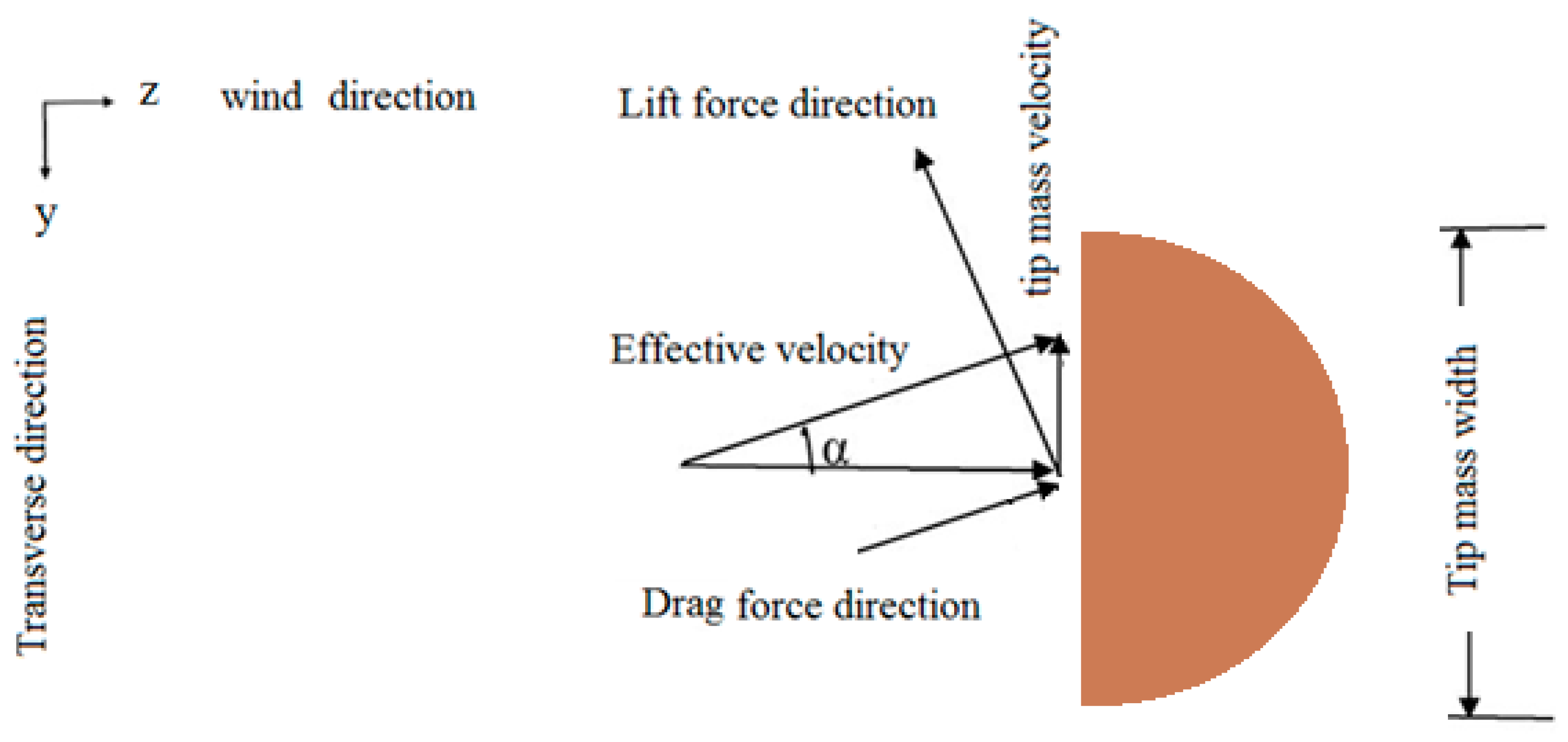
2.2. Aerodynamic Modeling

The flow-induced vibrations are divided into two parts as forced vibrations (vibrations in the along-wind direction) and self-induced vibrations (or aeroelasticity due to vibrations in the across-wind direction). Examples of forced vibrations are gust (turbulence effects), buffeting, and vortex shedding (without “lock-in” effect), and examples of induced vibrations are vortex shedding (with “lock-in” effect), pipeline vibration nearby of the bed, galloping, and bridge flutter. For the normal structures, the dynamic forces that must be considered based on engineering codes are the forces in the wind direction (usually turbulence and gusts), and vortex-induced oscillations such as flutter and galloping are, as a whole, of no real importance. Although there is no detailed explanation of galloping in the American Society of Mechanical Engineers (ASME) Code, vibrations in the galloping effect were shortlisted as a possible cause of the Tacoma Narrows bridge failure in 1940 between the vibrations induced by fluid flow. The galloping, which in some references is referred to as “dancing vibrations”, also appears in the vibrations of group of tethers or risers on a tension-leg platform, vibration of asymmetric ice-coated power lines, and the vibration of a flow line connected to the leg of an offshore tower, which are considered examples of galloping in engineering problems.
In practice, structures always experience conditions of turbulent flow. Bearman et al. [21] performed some experiments on the flow-induced vibration of a square-section cylinder and measured the aerodynamic damping. They showed that galloping instability and vortex resonance (due to negative aerodynamic damping) in some profiles is influenced by the turbulence of the airflow (e.g., in a wind tunnel test or natural winds). The nonlinear aeroelastic behavior of the system causes the failure of the prediction of galloping oscillation scales. Also, suitably choosing an aerodynamically equivalent reference frame with the unsteady situation that symbolizes the steady condition is another problem. Models of the combined effects of vortex-induced oscillation and galloping are presented by Corless et al. [22,23,24]. They considered combined effects to capture the measured values of the amplitude of vibrations. Also, Laneville and Parkinson [25] showed that the difficulty of calculating that value (by wind tunnel tests on galloping of bluff cylinders) is due to the turbulence damping effects which increase the Scruton number. Wind-induced aeroelastic instability of towers and structures (as a nonlinear oscillator) are mathematically modeled through the works of Parkinson et al. [26,27,28,29,30,31,32].
Parkinson [26] discovered that the criterion for the quasi-steady assumption is that any wake impact experienced by the oscillating body through one period should not affect the next period of the motion of the body. It means that, if the body (with characteristic length of D and exposed to free stream velocity of V) vibrates with the natural frequency of fn (for a low frequency, it typically is about one Hertz) exposing a fluid vortex impact at the beginning of a period of galloping, the vortex in fluid (with the center velocity of V) should be moved downstream adequately far away (at minimum, ten times the characteristic length of body) until the end of that period. Since, at one period later when the mass body returns to the location of the beginning of galloping, that vortex no longer disturbs the fluid flow around the body (fn V/10D). Meanwhile, the frequency disturbance to the mean flow generated by vortex shedding frequency (fS = V/5D) should be, at minimum, two times greater than the oscillation frequency. Bearman et al. [21] have a more conservative limit for the natural frequency of the square prism structure (fn V/30D). It means that the frequency disturbance to the mean flow generated by the vortex shedding frequency should be, at minimum, six times greater than the natural oscillation frequency of the structure for the quasi-steady supposition to be appropriate.
To obtain the force terms of the right-hand side of Equation (5) from Equation (2), the following is performed:
Based on the free body diagram of the y-z plane, which is depicted in Figure 2, the force is as follows:
F t i p = 1 2 ρ a V 2 D L r 0 L r [ c L cos α + c D sin α ] d s
Similarly, momentum is as follows:
M t i p = 1 2 ρ a V 2 D L r 0 L r s [ c L cos α + c D sin α ] d s
which can be obtained by application by the wind on the tip mass. Table 2 presents the experimental coefficients. As the lift and drag coefficients are known, the galloping force coefficient based on the angle of the wind normal to the surface (angle of attack) is obtained from the projection of lift and drag forces on the y-direction as follows:
C y = c L cos α + c D sin α
in which the angle of wind normal to the surface (angle of attack) is defined by
α = arctan ( w L + s w L V )
In the literature for commonly employed bluff bodies, the galloping force is given in the form of a third-order polynomial function as a function of the galloping position [13]. The first three aerodynamic coefficients are usually used to characterize the galloping force with zero coefficients for even terms:
F y = 1 2 ρ a V 2 D L r [ a 1 ( y ˙ V ) + a 3 ( y ˙ V ) 3 ]
where a1 and a3 are aerodynamic empirical coefficients, for which the D-shaped and other cylindrical cross sections are found in Table 2. The force terms in Equation (2) are replaced by the terms appearing in Equation (4) by the integration of Fy over the tip mass:
y t i p = w L + s w L
where s is from 0 to Lr. The effective wind momentum over tip mass is calculated around the beam free end.

2.3. Piezoelectric Modeling

There are different ways of explaining the basic equations of the piezoelectric materials based on which variables are of interest. Matrix relationships are extensively used for finite element modelling. For analytical approaches, some of the relations are commonly valuable so the problem can be shortened. For example, matrix relationships describe strain in direction 3 as a function of stress and field. To obtain the piezoelectric sensing voltage part of the formulation in the right-hand side of Equation (5) from Equation (2), the following is performed:
First, the Gauss law over the piezoelectric sheets is considered:
V ( t ) R   = d Q d t
where R is a purely resistive load to harvest the produced electrical energy. In the current study, the internal resistance is neglected with respect to the load resistance. It is an appropriate AC circuit for initial evaluation of the electrical responses; therefore, it is repeatedly employed in the literature. The charge accumulated by the surface electrodes is found by surface integration (all over the two electrodes, i.e., 2wpLp) from the electric displacement:
Q = D . n   d A
The vector of electric displacement appeared in Equation (12) in 3–1 mode is simplified to a scalar. The constitution equation of the piezoelectric is as follows:
D = ε 33 E + E p d 31 ε
which shows the relation between the electric displacement vector and the electrical field vector. In the current study, by use of the 3–1 mode, the matrix formulation is simplified to the scalar formulation. The vector of the electric field is simplified to a scalar as follows:
E = V t p
Strain at the top surface of each piezoelectric sheet (electrode) is evaluated from the following:
ε = ( t p + t b 2 ) 2 w x 2
In some references, it is referred to as the membrane strain of piezoelectric materials and is the axial strain at the center of the piezoelectric material. By replacing definitions of strain at the top surface and electric field through piezoelectric materials from Equations (14) and (15) in the definition of electric displacement (Equation (13)), the electric charge accumulated at the top surface of piezoelectric sheets covered by an electrode can be estimated. The time difference of electric charges is used in the right-hand side of Equation (12) to find the balance between the voltage of the electrode and beam displacement as follows:
[ 2 ε 33 w p L p t p ] V ˙ ( t ) + V ( t ) R   + i [ ( ϕ i ( L p ) ϕ i ( 0 ) ) E p d 31 w p ( t p + t b ) ] q ˙ i ( t ) = 0
The first term in the above equation is the electrical current through the two piezoelectric sheets with the capacitance of C p = 2 ε 33 w p L p t p ; the second term in the above equation is the electrical current through the impedance of electrical load connected to the piezoelectric sheets to harvest the energy; and the third term represents the effect of the rate of electrical charge accumulated on electrode surfaces. Detailed proof of Equation (16) is in Appendix A4.

2.4. Approximate Method

In this study, an approximate method is used to solve the problem:
ϕ ( x ) = ϕ ( L ) x 2 ( 3 L x ) 2 L 3
The approximation used in Equation (17) is obtained from the static deflection of the clamped, free beam in the static condition under the unit tip force applied at the free end. It is good to notice that, in Reference [9], Sirohi and Mahadik used a single cubic shape function for beam deflection. Furthermore, the proposed function of Equation (17) is not completely satisfying Equation (3) as it is just an approximation to the exact solution. As shown in Figure 3, that function is in good agreement with the final solution by the finite element method [13] with less complexity. Based on the single and parabola shape functions, which is assumed to represent the beam shape, its first derivate versus location is derived as follows:
ϕ ( x ) = ϕ ( L ) 3 x ( 2 L x ) 2 L 3
The effective values of system stiffness, which is obtained from the potential energy (strain energy) of the device, is as follows:
P . E = 1 2 0 L E I ( 2 w x 2 ) 2 d x = K e f f 2 w L 2
The effective mass, which is obtained from the kinetic energy of the system, is as follows:
K . E = 1 2 0 L ρ A w ˙ 2 d x + 1 2 0 L r ρ t i p A t i p y ˙ t i p 2 d s = M e f f 2 w L 2 ω 2
ytip can be evaluated from Equation (10). The explicit form of the effective mass is found from the following:
M e f f = m b [ Φ M ( L ) Φ M ( 0 ) ] + 2 m p [ Φ M ( L p ) Φ M ( 0 ) ] + m t i p [ 1 + 2 γ ] + 9 I t i p 4 L 2
Detailed proof of Equation (21) is in Appendix A2. The explicit form of the effective stiffness is given by the following:
K e f f = k b [ Φ K ( L ) Φ K ( 0 ) ] + 2 k p [ Φ K ( L p ) Φ K ( 0 ) ]
Detailed proof of Equation (22) is in Appendix A1. The dimensionless function of mass effect versus location is as follows:
Φ M ( x ) = ( ϕ ( x ) ϕ ( L ) ) 2 d ( x L ) = x 5 ( 5 x 2 35 L x + 63 L 2 ) 140 L 7
The dimensionless function of stiffness effect versus location is as follows:
Φ K ( x ) = L 3 ( ϕ ( x ) ϕ ( L ) ) 2 d x = 3 x L 3 [ x 2 3 L x + 3 L 2 ]
where the stiffness constants of the components (beam and piezoelectric sheet) as a function of physical and geometrical characteristics are as follows:
k p = E p w p t p 3 12 L b 3 + E p w p 3 L b 3 [ ( t p 3 + t b 2 ) 3 ( t b 2 ) 3 ]
k b = E b w b t b 3 12 L b 3
The mass constants of the components (tip, beam, and piezoelectric sheet) as a function of physical and geometrical characteristics are as follows:
m b = 0 L ρ A d x = ρ b w b t b L b
m p = 0 L p ρ p A p d x = ρ p w p t p L p
I t i p = 0 L r ρ t i p A t i p s 2 d s = m t i p L r 2 3
where the γ ratio is defined by the following:
γ = L r ϕ ( L ) ϕ ( L ) = 3 L r 2 L
Equation (21) contains all the dynamic mass effect caused by the tip mass and its mass moment of inertia, while the authors in Reference [9] (See Equation (26) in Reference [9].) missed the coupling of deflection and rotation term, i.e., m t i p 2 γ . The first term of Equation (21) presents the effect of the beam material. The second term of Equation (21) presents the effect of piezoelectric sheets on the effective mass. Here, they started from the clamped point until the length of Lp. The third term of Equation (21) presents the tip mass effect and the cross effect of rotation and displacement. The last term presents the effect of rotation (i.e., K . E r o t = 9 I t i p 4 L 2 w ˙ L 2 2 = I t i p w ˙ L 2 2 ). The election of the dimensionless mode shape (in Equation (17)) will affect the dimensionless derivate of the mode shape (See Equation (18).), which is used to calculate piezoelectric coupling terms (See Equation (3).), and the effective mass and stiffness distribution, which is used to evaluate the natural frequency of the system. Based on those functions which can be plotted as a function of the dimensionless variable (x/L), the calculations of the system can be performed.
Figure 3 presents the dimensionless function for calculating effective mass, effective stiffness, and the electromechanical coupling coefficient. Figure 3 is a general figure that can be used to assess the composite beams where its elasticity and mass distributions are the functions of the position. As shown, as the location of the stiffener element becomes closer to the clamped end, it is more effective (90 percent of the effectiveness of stiffness is at the left half of the beam, and 50 percent of it is located at the first 20 percent of the position) and, as the location of the mass element becomes closer to the free end, it is more effective (90 percent of the effectiveness of the mass is at the last 40 percent of the beam, and 50 percent of it is located at the last 20 percent of the position). For the cantilever beam with constant force at the free end considered here, the endpoint values can be calculated from Equation (18) which one can obtain the explicit expression as follows:
ϕ ( L ) = 3 2 ϕ ( L )
From Equations (23) and (24), they can be calculated as follows:
Φ M ( L ) = 0 . 2357
Φ K ( L ) = 3
As mentioned before, the selected approximate solution (See Equation (17).) follows the case where it is the static solution of the cantilever beam with a concentrated tip force. This lumped parameter model has identical efficiency with the distributed parameter model as it is degraded from the distributed parameters. It is good to notice that the fundamental frequency of the system could be found from the following:
ω = K e f f M e f f
Although the natural frequency could be found from Equation (11) as ϕ ( L ) exists in both the nominator and denominator, it is needed for the next calculations. The coefficient ϕ ( L ) is obtained by normalizing the effective mass to unity as follows:
ϕ ( L ) = 1 M e f f

2.5. Analytical Solution

Substituting the approximate solution from Equation (17) in governing Equations (4) and (16) by considering only one mode, the equations of the system are simplified as follows:
w ¨ L + 2 ξ ω w ˙ L + ω 2 w L =   [ L p ( 6 L 3 L p ) 2 L 3 M e f f E p d 31 w p ( t p + t b ) ] V ( t ) + ρ a V D a 1 w ˙ L L r 2 M e f f [ 1 + γ + γ 2 3 ] + ρ a D a 3 w ˙ L 3 L r 2 M e f f V [ 1 + 2 γ + 2 γ 2 + γ 3 + γ 4 5 ]
[ 2 ε 33 w p L p t p ] V ˙ ( t ) + V ( t ) R   + [ L p ( 6 L 3 L p ) 2 L 3 E p d 31 w p ( t p + t b ) ] w ˙ L ( t ) = 0
Detailed proof of Equation (34) is in Appendix A3. The analytical solution of the above system of equations (i.e., Equations (34) and (35)) in steady-state operation is proposed as a trigonometric function of time with the same frequencies:
w ( x , t ) = w max x 2 ( 3 L x ) 2 L 3 sin ( ω t )
V ( t ) = V max sin ( ω t + φ )
where t is the time, x is the location through the beam measured from the clamped end, L is the length of the beam, wmax is the maximum deflection of the beam which occurs at the free end, Vmax is the maximum produced voltage by the piezoelectric sheets, ω is the angular velocity of the galloping motion, and φ is the phase difference between the tip motion and voltage production.
Replacing the assumptions of Equations (36) and (37) in Equation (35) and integrating both sides of the resulting equation from time instant 0 to time instant T/2, where the T is the period of motion, the relationship between wmax and Vmax is obtained as follows:
V max = 3 ( 2 L L p ) L p ( t p + t b ) w p E p d 31 R ω 2 L 3 1 + ( 2 ε 33 w p L p t p R ω ) 2 w max
Multiplying Equation (33) by wL and Equation (34) by V, integrating the resulting equations concerning time from instant 0 to T/2 (time duration as half the period), and equating the coupling terms between two equations gives the following:
w max = 2 ξ ω M e f f + R [ 3 E p d 31 w p ( t p + t b ) L p ( 2 L L p ) 2 L 3 ] 2 1 + ( 2 ε 33 w p L p t p R ω ) 2 ρ a V D L r a 1 2 [ 1 + γ + γ 2 3 ] 3 8 ω 2 ρ a D L r a 3 2 V [ 1 + 2 γ + 2 γ 2 + γ 3 + γ 4 5 ]
It is good to notice that, in integrating from 0 to T/2, there is no variation in kinetic energy (first term in Equation (33)), elastic energy (third term in Equation (33)), and the energy stored in capacitance (first term in Equation (33)) since they will not appear in the final equations (i.e., equation of energy balance).
Also, the other coefficient that affects the value open circuit obtained from Equation (38) in case of connecting to a load resistance is the phase difference, which is defined by a phase difference of voltage and tip mass position as follows:
φ = arctan ( 1 2 ε 33 w p L p t p R ω )
Derivation of Equation (46) is straightforward from putting the values of voltage and displacement at the initial time (i.e., w ˙ = w max ω , V = V max sin ( φ ) , and V ˙ = ω V max c o s ( φ ) ) into Equation (34). The effect of the phase difference between voltage and displacement on the value of the load-connected circuit to the voltage of the open circuit is obtained from Equation (38) and is as follows:
V max w max = V max w max | R cos ( φ )
By applying the condition of a positive value under the square root, the onset of galloping (minimum value of the velocity where the expression under square root is positive) is derived from Equation (39) and is as follows:
V o n s e t = 4 ξ ω M e f f + 2 R [ 3 E p d 31 w p ( t p + t b ) L p ( 2 L L p ) 2 L 3 ] 2 1 + ( 2 ε 33 w p L p t p R ω ) 2 ρ a D L r a 1 [ 1 + γ + γ 2 3 ]
Based on the definition of the onset of galloping in Equation (42), the maximum tip deflection of the beam (See Equation (39).) is rearranged as a function of the velocity:
w max = V o n s e t ω a 1 [ 1 + γ + γ 2 3 ] 3 4 a 3 [ 1 + 2 γ + 2 γ 2 + γ 3 + γ 4 5 ] ( V V o n s e t 1 ) V V o n s e t
Equation (43) in the current study is equal to Equation (18) in Reference [15] in the limit of a concentrated tip mass ( γ 0 ) and in considering the Taylor expansion of the arctangent function where a 3 = a 1 3 . The average harvested power over time ( P a v e = V max 2 2 R ) is obtained by integrating the power during a period of motion:
P a v e = ( ( 2 L L p ) L p ( t p + t b ) w p E p d 31 ) 2 R L 6 ( 1 + ( 2 ε 33 w p L p t p R ω ) 2 ) 3 a 1 [ 1 + γ + γ 2 3 ] a 3 [ 1 + 2 γ + 2 γ 2 + γ 3 + γ 4 5 ] V o n s e t 2 ( V V o n s e t 1 ) V V o n s e t

2.6. A Note on Coupling Term

Another value which is reported in the literature is the value χ:
χ = L p ( 6 L 3 L p ) 2 L 3 M e f f E p d 31 w p ( t p + t b )
where χ is the static coupling factor of the considered mode (i.e., k31 transversal coupling factor in the driving part). This parameter could appear as a simpler coefficient of the voltage at the first term in the right-hand side of Equation (34). Since the measured output of the piezoelectric sensing device is usually less than the expected ideal value, the above value needs modification as follows:
χ c l a m p e d = χ t h e o r y η p i e z o
where η p i e z o is the performance of the piezoelectric at the clamped beam configuration in comparison with the ideal behavior. The performance of the piezoelectric at the clamped beam configuration is obtained in Reference [8] by use of the coefficient k 2 = E p d 31 2 ε 33 . The modification leads to the value of 0.2326 for the performance of the piezoelectric at the clamped beam configuration in comparison with the ideal behavior (See Equation (28) in Reference [8].). If the correction of the value of the capacity of the piezoelectric sheet in comparison with the static piezoelectric sheet is considered, the performance of the piezoelectric at the clamped beam configuration in comparison with the ideal behavior used in the coupling factor is obtained as follows:
η p i e z o = 1 E p d 31 2 ε 33
Based on that the definition of piezoelectric performance, Equation (4) for one mode and Equation (35) are restated as follows:
q ¨ + 2 ξ ω q ˙ + ω 2 q = η p i e z o χ V ( t ) +    ρ a V D a 1 q ˙ L r 2 M e f f [ 1 + γ + γ 2 3 ]                  + ρ a D a 3 φ L 4 q ˙ 3 L r 2 V [ 1 + 2 γ + 2 γ 2 + γ 3 + γ 4 5 ]
C p V ˙ + V R   + χ q ˙ = 0
which is similar to the Equations (27) and (28) in Reference [14]. The only difference with Reference [14] is the sign of χ, where in that reference, d31 is considered a positive value, while here, the negative sign is considered. The coupling factor has affected the performance of the system and is measured from the relation between displacement and produced voltage. The relation between the voltage and tip mass deflection in the open circuit case is proportional to the χ value. It can be found in Equation (38) that the voltage to displacement coefficient of the system at open circuit condition is as follows:
V max w max | R = 3 ( 2 L L p ) ( t p + t b ) t p E p d 31 4 L 3 ε 33
where lim a R 1 + b 2 R 2 | R = a b . As shown in Equation (50) for the offered configuration, the width of the piezoelectric sheet does not affect the performance of the system since in the engineering design, the width of the piezoelectric sheet could be as thin as possible (regarding other engineering limitations) to save the amount of material. Also, for the arbitrary set of discrete piezoelectric sheets, the above formulation can be rephrased as follows:
V max w max | R   = 6 ( t p + t b ) t p E p d 31 L 3 ε 33 ( L x a v e )  
where xave is the average distance between the piezoelectric sheet (midpoint of the piezoelectric sheet) from clamped point ( x a v e = x e + x i 2 ), xi is the minimum distance between the piezoelectric sheet (left of the piezoelectric sheet) from clamped point, and xe is the maximum distance between the piezoelectric sheet (right of the piezoelectric sheet) from clamped point. Detailed proof of Equation (51) is in Appendix A5. It is noticeable that Equation (50) is a specific case of Equation (51); by substitution of x a v e = L p 2 in Equation (51), Equation (50) is retrieved. Another point in Equation (50) is that the configuration of two piezoelectrics cause the same voltage-displacement relation as that of the single piezoelectric case. The reason is that the factor 2 in the nominator of the two moments generated by the piezoelectric sheets is reduced by factor 2 in the denominator of the series of capacitance (twice capacitor value). The conclusion from Equation (50) is the evaluation of the theoretical maximum harvesting power in the energy harvesting of a cantilever with an attached prism under aeroelastic galloping. Replacing the generated voltage in the case of connecting load resistance (See Equation (41).) and maximum displacement of the case of no damping (internal structural damping and the electrical damping) in Equation (50), the maximum voltage in the energy harvesting case is obtained as follows:
V max = 3 ( 2 L L p ) ( t p + t b ) t p E p d 31 4 L 3 ε 33 cos ( φ ) V o n s e t ω a 1 [ 1 + γ + γ 2 3 ] 3 4 a 3 [ 1 + 2 γ + 2 γ 2 + γ 3 + γ 4 5 ] ( V V o n s e t 1 ) V V o n s e t
Optimal wind velocity could be obtained from Equation (49) as follows:
V   o p t = 2 V o n s e t
If the above velocity is replaced in Equation (49) and the onset velocity is approximated from Equation (42) by the assumption of negligible electrical damping, the following equation is derived for optimal voltage:
V o p t = 3 ( 2 L L p ) ( t p + t b ) t p E p d 31 4 L 3 ε 33 ω cos ( φ ) 2 a 1 [ 1 + γ + γ 2 3 ] 3 4 a 3 [ 1 + 2 γ + 2 γ 2 + γ 3 + γ 4 5 ] 4 ξ ω M e f f ρ a D L r a 1 [ 1 + γ + γ 2 3 ]
At the phase difference of φ = π/4, the following value for optimal power is obtained:
P o p t = 12 ( ( 2 L L p ) ( t p + t b ) t p L 3 E p d 31 ε 33 ξ M e f f ρ a D L r a 3 [ 1 + 2 γ + 2 γ 2 + γ 3 + γ 4 5 ] ) 2 1 a 1 [ 1 + γ + γ 2 3 ]

3. Results and Discussion

Various aspects of the energy harvester are analyzed next to assess the properties of different parameters on the level of harvested energy. As a first stage, the numerical model is validated and compared with the experimental data performed by Sirohi and Mahadik [9].

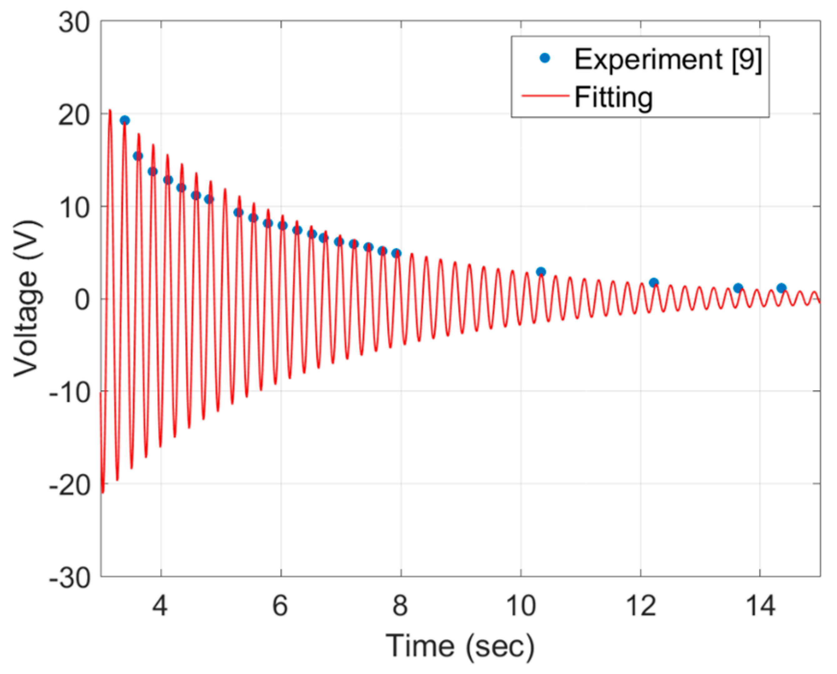
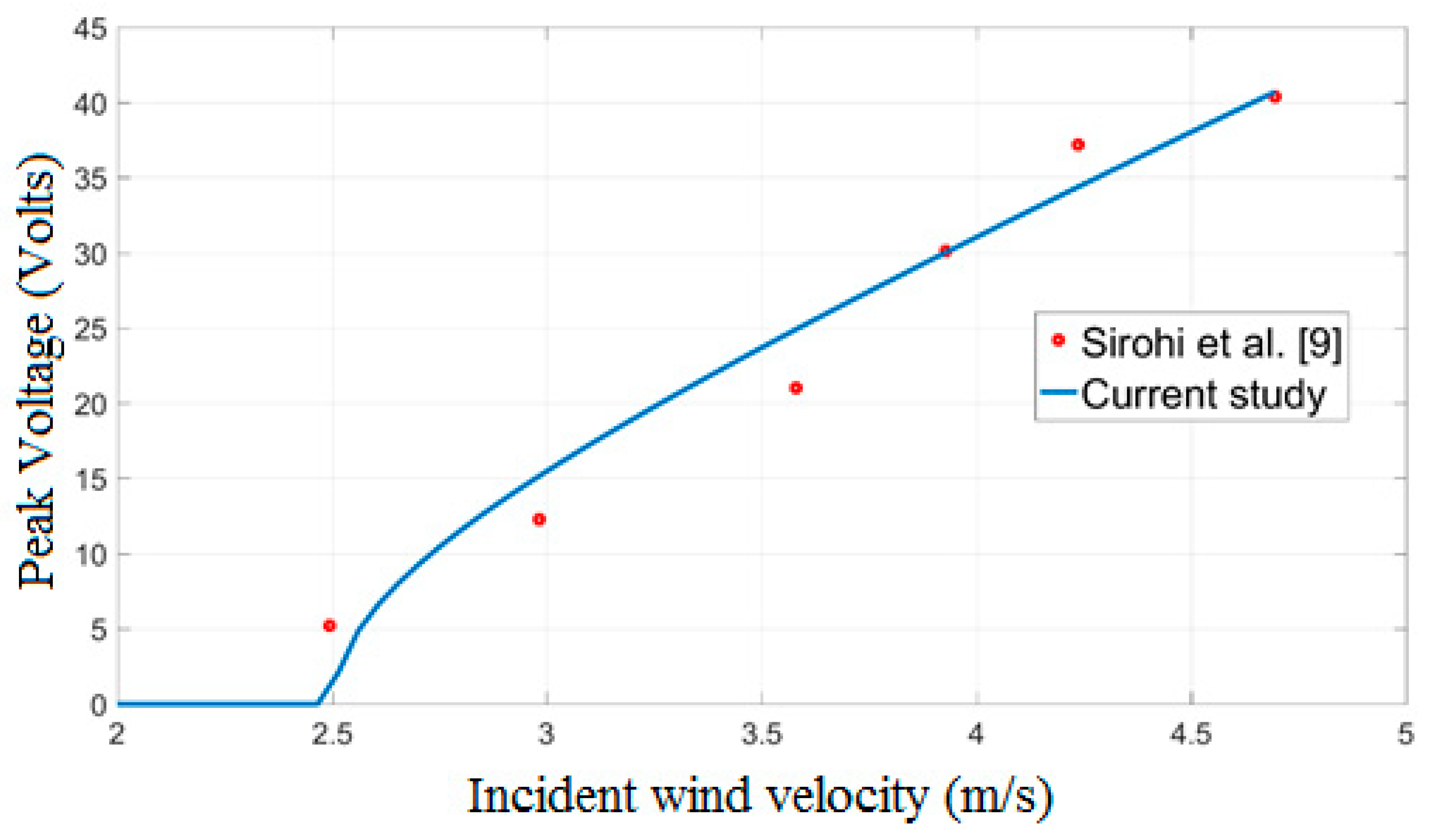
3.1. Validation by Experimental Results

Further, the evaluation of the damping ratio of the system is needed. The value ξ = 0.003 is used in Reference [14] (See page 251, Equation (28).), but here, Figure 9 of Reference [9] is used in the simulations. Figure 4 presents the evaluation of the damping ratio of the system from the measured impulse response of the beam with electrodes in an open circuit [9]. The estimated value by using the tip values of voltage presented in Figure 4 are ξ = 0.0109 and f = 4.17 (1/s).
The most important features of the numerical results and its comparison with the experimental results of Sirohi and Mahadik [9] is presented in Table 3. The results of the simulation of the system (of which the physical property is given in Table 1) with the aerodynamic coefficient given in Table 2 are summarized in Table 3. As shown in the calculation of natural frequency, the relative error of the used method is less than 2 percent while the relative error of the Galerkin procedure by Abdelkefi et al. [14] is more than 45 percent (See Table 2 in Reference [14].). They found that the angular velocity for the first mode is 38.176 which resulted in 6.076 Hz in frequency. Since the results of the approximate method have less error in comparison with the finite element method, this difference comes from the application of the first order Rayleigh–Ritz method instead of the higher-order modal method or Galerkin method used in Reference [14], which affect the difference in natural frequency and effective mass of the system.
Also, it is revealed in Table 3 that the onset of galloping (with the aerodynamic coefficients of Table 2) for the system based on the Equation (42) is predicted at 22.79 m/s. The value at load resistance (0.7 MΩ) is 40.9455 m/s, while for 9.5 mph (4.25 m/s), the value of 30 Volts (which is approximately a 2-mm tip deflection) is seen (See Figure 8 of Reference [9], and consider mph = 0.44704 m/s.). One conclusion of this paradigm could be that observed motion, in that case, is not a real galloping, and the coefficients of Table 2 are not recommended. Although the authors of References [13,14] solved this paradigm by using artificial values for the system damping ratio, they exposed unrealistic results for tip displacement in the next step. The aerodynamic coefficient values which fit the experimental results of Reference [9] are a1 = 7.2 and a3 = −2.1757. Additionally, the fitted results are present in Figure 5. The fitted coefficients predict the onset of galloping at 5.6 mph (2.5 m/s) for R = 0.7 MΩ, and the maximum error is less than 5 Volts.
Unfortunately, there is no published data other than References [9,16] for the problem of transverse galloping while the beam is normal to the wind direction and tip mass size in the direction of the beam (from clamped point to free end) is comparable to the beam length. More experiment results from Reference [17] are presented in Table 4 for validating the theoretical study and the numerical simulations. Those results are related to a tip mass of 23 g with length and width of 70 and 60 mm, respectively. Moreover, the range of wind velocity is 8–12 (m/s). Instead of a two-layer piezoelectric, Jamalabadi et al. [17] used one piezoelectric sheet partially covering the cantilever. The start point of the piezoelectric sheet was not the clamped point for some manufacturing considerations, and the piezoelectric sheet was located at the position with the highest strain values.
Table 5 presents the numerical and experimental results of Jamalabadi et al. [17]. As shown, the natural frequency of the system is evaluated at 7.33 Hz while the experimental data (first peak of frequency response) happens at 7.5 Hz (2 percent error).
It is good to note that, in some references, to remove the difference of the frequency gained by the numerical method and the measured frequency, a nonlinear torsional spring is considered at the clamped point for the effects of the incomplete clamp. In this study, the clamp point is considered a complete clamp condition. Also, the voltage to tip displacement of the system is evaluated with a good agreement (5 percent error), since the correction of Equation (47) is not necessary (if the correction of Equation (47) is applied, the relative error increases to 12 percent).
Figure 6 presents the variations of the voltage results of Reference [17] for different values of wind velocity. Inspecting this figure, the theory used here fits the experimental results for a1 = 2.416 and a3 = −201.3095.

3.2. Effects of the Load Resistance and Tip Mass Length Ratio on the Harvester′s Response

The effect of tip mass length on effective mass is plotted in Figure 7. The curve is plotted by use of Equation (21). As shown, if the dynamic correction is not applied on the tip mass, it will lead to a higher error in the calculation of effective mass, natural frequency, etc. After the correction of Figure 8 in calculating the effective mass, it would be ready to be used in design calculations provided for the lumped method, as presented in Reference [7]. For example, in the case investigated in this paper, for the tip mass length to beam length ratio ( γ = L r L ) of 2.61, the contribution of tip mass in the effective mass is 13.95 times of its static mass. It means the total mass of the system is approximately 14 times the static mass of the tip mass. If the formulation in Reference [9] is adopted, the value is 6.1 instead. Also, it is revealed in Figure 8 that, if the length of the rigid tip body is ten times that of the cantilever length, the effective mass should be considered in vibrational calculations and is one hundred times the mass of the tip body.
The theoretical relation between the open-circuit voltage and the tip displacement as predicted by Equation (43) is about 570.1643 volts per each meter deflection of the tip of the beam. These values will be corrected by the phase difference angle of 3.9477 degrees which leads to the correction of 568.8111 volts per meter. It means that the maximum voltage of 34 corresponds to the deflection of 6 centimeters of tip deflection. If the correction of Reference [9] is considered, this value decreases to 46 mm, while as the measurement of deflection is not reported in Reference [9], it could not be compared with experimental data.
The added damping ratio by applying the electrical impedance is shown in Figure 9. The effective damping ratio as a function of load resistance is as follows:
ξ e l e c = R [ 3 E p d 31 w p ( t p + t b ) L p ( 2 L L p ) 2 L 3 ] 2 ( 2 ω M e f f ) ( 1 + ( 2 ε 33 w p L p t p R ω ) 2 )
Figure 9 presents the equivalent damping ratio of the electrical load impedance as a function of load impedance. As shown, the minimum added damping ratio to the system at a load resistance of 0.7 MΩ is 0.01. The artificial value of 0.003 for total damping ratio at that point could not be considered. As one can observe from Equation (39), the damping coefficient should have a maximum value at a specific configuration:
R o p t = t p 2 ε 33 w p L p ω
At this value of resistance, the phase difference of voltage and displacement would be π/4 and the electrical damping is maximized. Figure 9 presents the peak value when the value (R = 57 kΩ) is less than the initial range used in the experiment of Reference [8].
To compare the power harvested in Reference [13] with the current study, the electrical damping is defined as follows:
C = R 1 + ( C p R ω ) 2 ( η p i e z o χ ) 2
where C is defined as the electrical damping resulting from the electromechanical coupling by Tan and Yan under Equation (5) in Reference [13], θp (here is η p i e z o χ ) is adopted by comparing their Equation (1) with Equation (48), and C p = 2 ε 33 w p L p t p . By observation in Equation (56), it is clear that, if the electrical damping ratio defined in Equation (56) is multiplied by angular velocity, the electrical damping defined in Equation (58) is obtained (C = 2ωζe). If harvested power is considered during a period of motion
P max = ξ e M e f f ω R 2 2 ( ξ + ξ e ) ω M e f f ρ a V D L r a 1 2 [ 1 + γ + γ 2 3 ] 3 8 ρ a D L r a 3 2 V [ 1 + 2 γ + 2 γ 2 + γ 3 + γ 4 5 ]
and rearranged by the definition of Equation (58), harvested power is
P max = 4 M e f f C V 3 R 2 ω 2 M e f f ( 4 ξ ω + 2 C ) ρ a D L r V a 1 [ 1 + γ + γ 2 3 ] a 3 [ 1 + 2 γ + 2 γ 2 + γ 3 + γ 4 5 ]
As seen from the above equation, Equation (58) does not presents an explicit expression of harvested power as a function of C because, in Equation (58), R is still a function of C (See Equation (58).). The effects of electrical damping on the harvested power are presented in Figure 10. For the configuration defined in Table 1, the maximum value of C is 3.9722. Figure 8 reveals that even such odd wind velocities can be accessible for steady power harvesting; the amount of harvested power could not exceed 100 milliwatts. The resultant harvested power of the current case with that of References [13,14] based on the coefficient of Table 2 could be compared in Figure 10.
In the current study, the analytical solution is compared with some previous cases and it is expected that the model is useful for low-amplitude energy harvesting which is in the range of linear elastic material strain. As shown, the experimental results demonstrate that the values in Table 2 are not valuable in the calculation of harvested power for the low-amplitude galloping regime. The a1 value found in this study is considerably higher than the a1 value presented in Table 2. This estimates the onset of galloping velocity much lower than that in the experimental results (See Equation (42)). Also, the a3 coefficient is 1 order to 2 orders of magnitude higher than the a3 presented in Table 2. Even the difference in estimation of onset of galloping velocity ignores the 1–2 order of magnitude difference in a3 and could cause a one order of magnitude difference in final deflection (See Equation (39).) and voltage (See Equation (38).) and two orders of magnitude difference in power results (See Equation (44), and compare Figure 10 with Figure 4 of Reference [17]). The difference between fitted coefficient for Reference [9] (Re ≈ 104) and that of Reference [17] (Re ≈ 105) could be attributed to the various characteristic lengths and ranges of velocity which lead to various Reynolds numbers. While the Reynolds number for Reference [9] is about 11,400 the Reynolds number for Reference [17] is about 67,260. It shows that, to globalize the results of the aerodynamic coefficient to the problem of beam galloping perpendicular to the wind direction, more experiments are needed.

4. Conclusions

In this study, galloping of two piezoelectric layers attached to a cantilever beam with a tip mass exposed to the wind free stream was studied. The fluid–solid interaction Equations are solved analytically by use of the approximation method. The resulting model is confirmed by preceding experimental results. The effects of the tip mass length ratio on the onset of galloping, the level of the produced voltage, and harvested power are determined. In this research are the following:
  • In this study, a simple analytical model is used to encounter the effect of a tip mass which could be used by engineers for design of energy harvesting devices with piezoelectric materials.
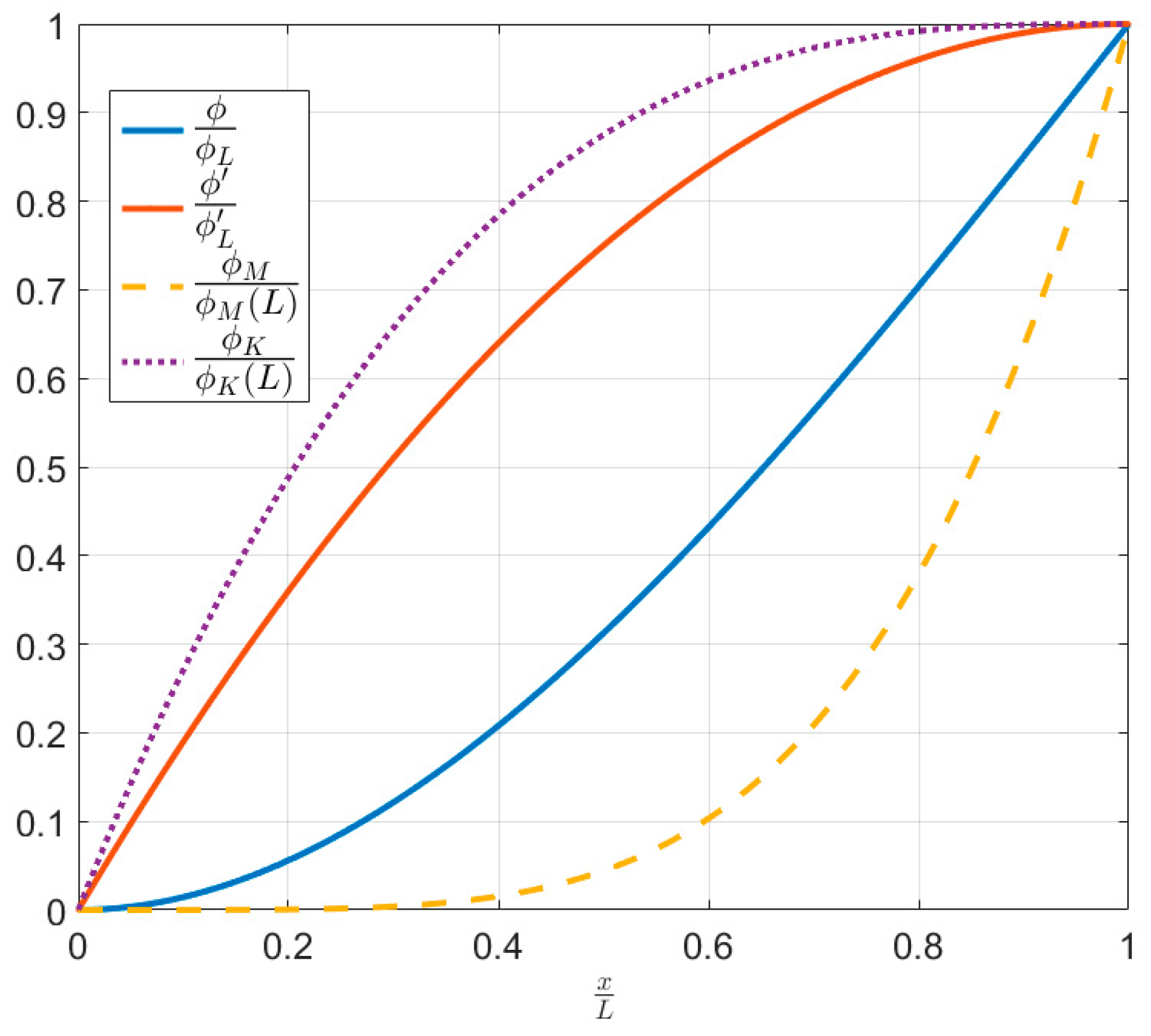
  • The dimensionless functions for calculation of effective mass, effective stiffness, and electromechanical coupling coefficient were presented.
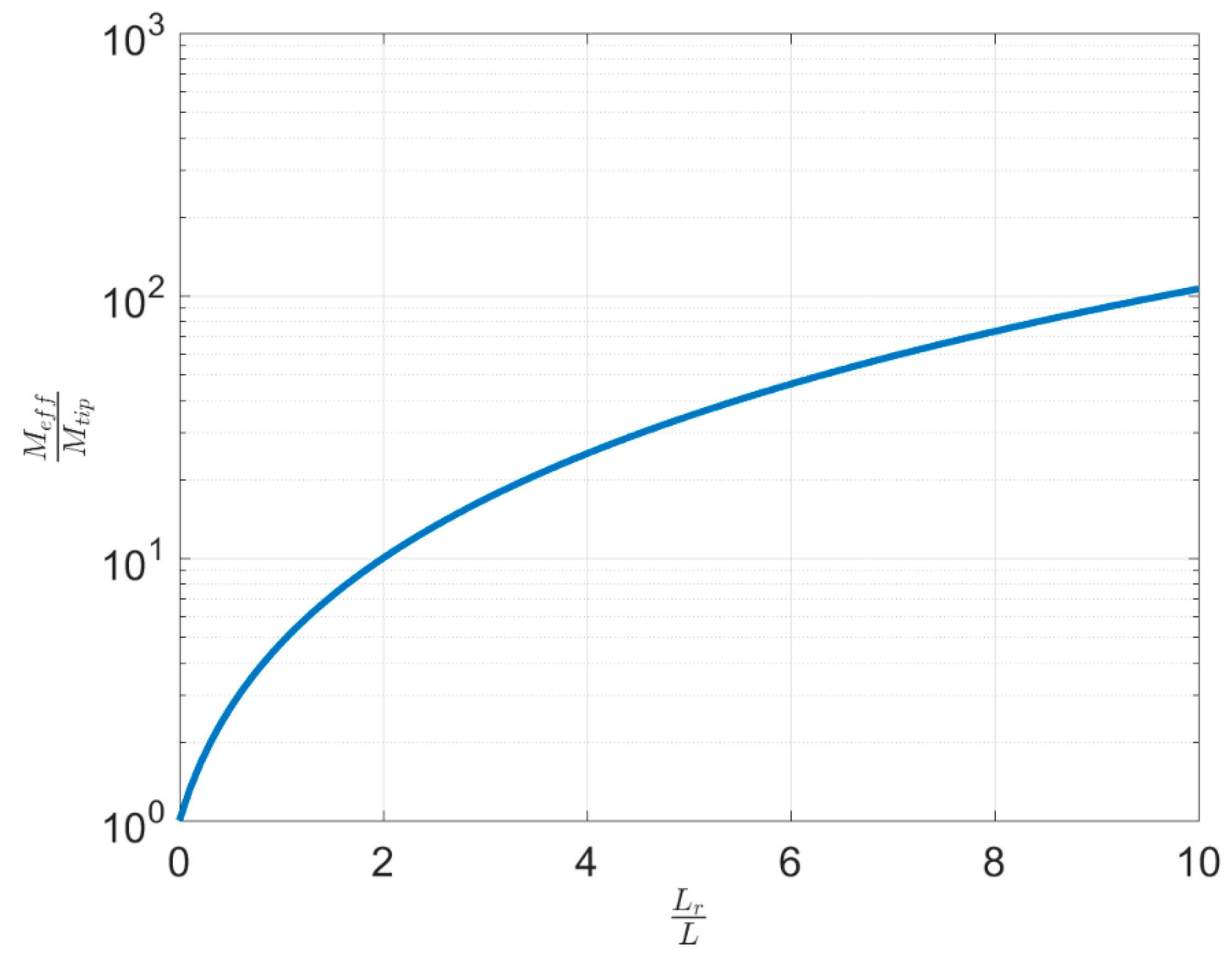
  • The effect of tip mass length on effective mass was developed.
  • The onset of galloping for the system was predicted analytically.
  • The current aerodynamic coefficient in the literature causes great numerical errors.
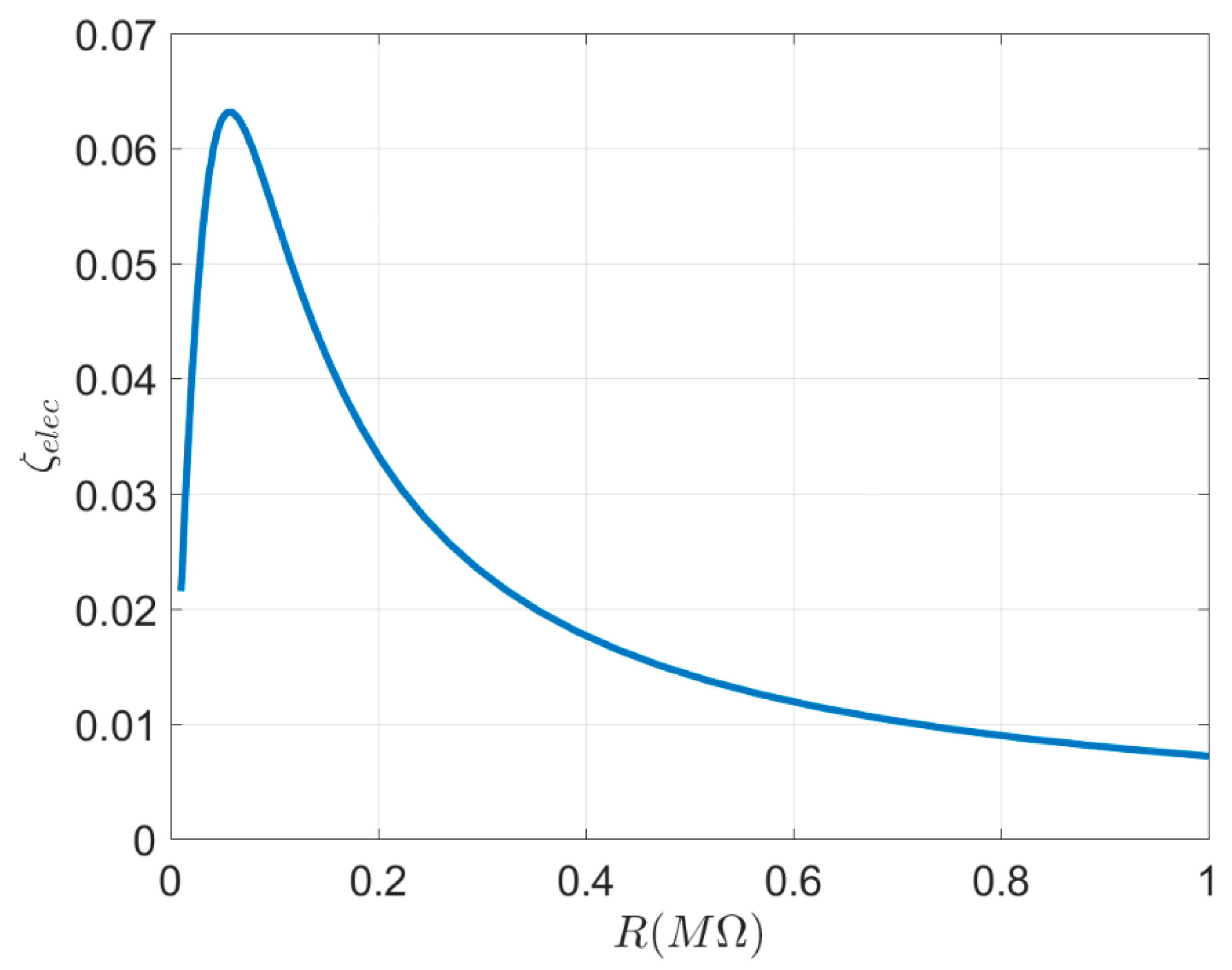
  • The equivalent damping ratio of the electrical load impedance as a function of load impedance was calculated.
  • The effect of tip mass on the analytical solution of the concentrated mass was calculated.
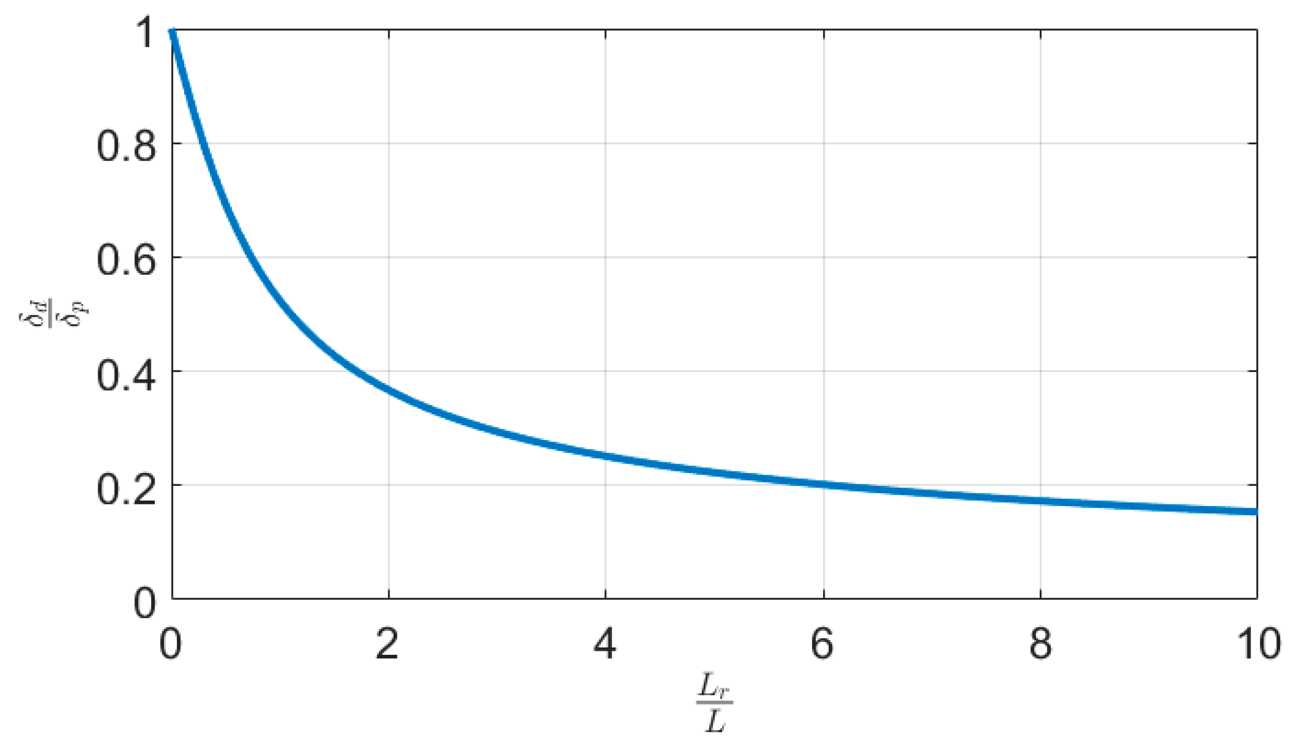
  • The effect of tip mass is a decrease in the tip displacement in comparison with the point mass.
  • The results are fitted on the analytical solution, and the new aerodynamics coefficients included the effect of tip mass.
  • As shown by increases of the length of tip mass for the constant beam and piezoelectric length, the inertia of the system increases while the tip displacement and onset of galloping decrease.

Conflicts of Interest

The author declares no conflict of interest.

Nomenclature

ρaAir density (kg·m−3)
mtTip mass (g)
LrLength of the tip body (mm)
DWidth of the tip body (mm)
VWind velocity (m/s)
LLength of the beam (mm)
wbWidth of the beam material layer (mm)
tbBeam material layer thickness (mm)
EbBeam material Young′s modulus (GN·m−2)
ρbBeam material density (kg m−3)
xpStart of the piezoelectric sheets (mm)
LpLength of the piezoelectric sheets (mm)
wpWidth of the piezoelectric layer (mm)
tpPiezoelectric layer thickness (mm)
EpPiezoelectric material Young’s modulus (GN m−2)
ρpPiezoelectric material density (kg m−3)
d31Strain coefficient of the piezoelectric layer (pC N−1)
ε33Permittivity component at constant strain (nF m−1)
mbBeam mass (g)
mpPiezoelectric sheet mass (g)
meffTotal mass (g)
kbBeam stiffness (N/m)
kpPiezoelectric sheet stiffness (N/m)
keffTotal stiffness (N/m)
fnNatural frequency (1/s)
fexpExperimental natural frequency (1/s)
CpTotal capacitance of the piezoelectric layers (nF)
χCoupling factor (mmCm−1·kg−1/2)
VmVoltage of the piezoelectric layers (V)
wTip displacement of the beam (m)
vonsetOnset of the galloping velocity (ms−1)

Appendix A

Appendix A1. Find the Effective Stiffness of the System

As mentioned before, the effective values of the system’s stiffness are obtained from the potential energy (strain energy) of the device (See Equation (19).). Assuming the approximate solution of Equation (17) for one mode, the second derivate of the beam displacement is as follows:
2 w ( x , t ) x 2 = 3 L x L 3 ϕ L q ( t )
where ϕ L = ϕ ( x = L ) . By substitution of the second derivate of the beam displacement into the potential energy (strain energy) of the system presented in Equation (19) and considering the definitions in Equations (24)–(26), the potential energy of the beam is obtained as follows:
P . E = K e f f 2 w L 2 = K e f f 2 ( ϕ L q ( t ) ) 2 = 1 2 0 L E I 2 d x = 1 2 0 L E b I b ( 2 w x 2 ) 2 d x + 0 L p E p I p ( 2 w x 2 ) 2 d x = 1 2 0 L E b I b ( 3 L x L 3 ϕ L q ( t ) ) 2 d x + 0 L p E p I p ( 3 L x L 3 ϕ L q ( t ) ) 2 d x = ( ϕ L q ) 2 ( E b I b 2 L 3 0 L 9 L 3 ( L x ) 2 d x + E p I p L 3 0 L p 9 L 3 ( L x ) 2 d x ) = ( ϕ L q ) 2 ( k b 2 0 L 9 L 3 ( L x ) 2 d x + k p 0 L p 9 L 3 ( L x ) 2 d x ) = ( ϕ L q ) 2 ( k b 2 0 L 9 L 3 ( L x ) 2 d x + k p 0 L p 9 L 3 ( L x ) 2 d x ) = ( ϕ L q ) 2 ( k b 2 [ 3 x L 3 [ x 2 3 L x + 3 L 2 ] ] 0 L + k p [ 3 x L 3 [ x 2 3 L x + 3 L 2 ] ] 0 L p ) = k b [ Φ K ( L ) Φ K ( 0 ) ] + 2 k p [ Φ K ( L p ) Φ K ( 0 ) ] 2 ( ϕ L q ( t ) ) 2
whereby comparing the first and last rows, Equation (22) is obtained.

Appendix A2. Find the Effective Mass of the System

As mentioned before, the effective values of the system’s mass are obtained from the kinetic energy of the device (See Equation (20).). Assuming the approximate solution of Equation (17) for one mode, the first derivate of displacement of the beam versus time is obtained as follows:
w ˙ ( x , t ) = ϕ L q ˙ ( t ) x 2 ( 3 L x ) 2 L 3
where ϕ L = ϕ ( x = L ) . Also, assuming the approximate solution of Equation (18) for one mode, the first derivate of the slope of the beam versus time is obtained as follows:
w ˙ ( x , t ) = ϕ L q ˙ ( t ) x 2 ( 3 L x ) 2 L 3
where ϕ L = ϕ ( x = L ) .
By substitution of the above equations into the kinetic energy of the system presented in Equation (20) and considering the definitions in Equation (10) (for the ytip), Equation (23) (for the dimensionless function of mass effect versus location), and Equations (27)–(30) (for mass constants of tip, beam, and piezoelectric sheet), the kinetic energy of the beam is obtained as follows:
K . E = M e f f 2 w ˙ L 2 = M e f f 2 ( ϕ L q ˙ ( t ) ) 2 = 1 2 0 L ρ A w ˙ 2 d x + 1 2 0 L r ρ t i p A t i p y ˙ t i p 2 d s = 1 2 0 L ρ b A b w ˙ 2 d x + 0 L p ρ p A p w ˙ 2 d x + 1 2 0 L r ρ t i p A t i p ( w ˙ L + s w ˙ L ) 2 d s = 1 2 0 L ρ b A b ( ϕ L q ˙ ( t ) x 2 ( 3 L x ) 2 L 3 ) 2 d x + 0 L p ρ p A p ( ϕ L q ˙ ( t ) x 2 ( 3 L x ) 2 L 3 ) 2 d x + 1 2 0 L r ρ t i p A t i p ( ϕ L q ˙ ( t ) + s 3 ϕ L q ˙ ( t ) 2 L ) 2 d s = ( ϕ L q ˙ ) 2 ( 1 2 0 L ρ b A b ( x 2 ( 3 L x ) 2 L 3 ) 2 d x + 0 L p ρ p A p ( x 2 ( 3 L x ) 2 L 3 ) 2 d x ) + ( ϕ L q ˙ ) 2 ( 1 2 0 L r ρ t i p A t i p ( 1 + 3 s 2 L ) 2 d s ) = ( ϕ L q ˙ ) 2 ( 1 2 0 L ρ b A b x 4 ( 3 L x ) 2 4 L 6 d x + 0 L p ρ p A p x 4 ( 3 L x ) 2 4 L 6 d x ) + ( ϕ L q ˙ ) 2 ( ρ t i p A t i p 2 [ 1 + 3 s L + 9 s 2 4 L ] 0 L r ) = ( ϕ L q ˙ ) 2 ( 1 2 0 L ρ b A b x 4 ( 9 L 2 6 L x + x 2 ) 4 L 6 d x + 0 L p ρ p A p x 4 ( 9 L 2 6 L x + x 2 ) 4 L 6 d x ) + ( ϕ L q ˙ ) 2 ( ρ t i p A t i p L r [ 1 2 + 3 L r 2 L + 3 L r 2 8 L 2 ] ) = ( ϕ L q ˙ ) 2 ( ρ b A b L 2 0 L 9 L 2 x 4 6 L x 5 + x 6 4 L 7 d x + ρ p A p L 0 L p 9 L 2 x 4 6 L x 5 + x 6 4 L 7 d x ) + ( ϕ L q ˙ ) 2 ( ρ t i p A t i p L r [ 1 2 + 3 L r 2 L ] + 9 I t i p 8 L 2 ) = ( ϕ L q ˙ ) 2 ( m b 2 [ x 5 ( 5 x 2 35 L x + 63 L 2 ) 140 L 7 ] 0 L + m p [ x 5 ( 5 x 2 35 L x + 63 L 2 ) 140 L 7 ] 0 L p ) + ( ϕ L q ˙ ) 2 ( m t i p 2 [ 1 + 2 γ ] + 9 I t i p 8 L 2 ) = m b [ Φ M ( L ) Φ M ( 0 ) ] + 2 m p [ Φ M ( L p ) Φ M ( 0 ) ] + m t i p [ 1 + 2 γ ] + 9 I t i p 4 L 2 2 ( ϕ L q ˙ ) 2
whereby comparing the first and last rows of Equation (A5), the Equation (21) is obtained.

Appendix A3. Find the Second-Order Governing Equation of Motion of the System

Neglecting the dynamic effects of the longitudinal forces and rotational inertia and considering the governing equation of transversal vibration of a beam as presented by Equation (2), one can use the equivalent method to solve the equation. If both sides of Equation (2) are multiplied by the essential mode shape and integrated all over the system, one can obtain for the essential mode the following:
0 L + L r ρ A ϕ 2 q ¨ d x + 0 L E I ϕ ϕ i v q d x + 0 L c I ϕ ϕ i v q ˙ d x =                     E p d 31 w p ( t p + t b ) V 0 L [ d d x δ ( x x 1 ) ] L 1 L 2 ϕ d x +                     M t i p 0 L d d x δ ( x L ) ϕ d x + F t i p 0 L δ ( x L ) ϕ d x
where the first term on the left-hand side is the inertial term of which the effective mass is found in Equation (21) by use of the method of energy
M e f f = 0 L ρ A ( φ φ L ) 2 d x + 0 L r ρ t i p A t i p ( 1 + s φ L φ L ) 2 d s
and where the second term is the effective stiffness which is found in Equation (19) by use of the method of energy
K e f f = 0 L E I φ 2 d x
while the integration is converted based on the following partial integral relation,
0 L φ φ i v d x = φ φ ] 0 L 0 L φ φ d x = φ φ ] 0 L φ φ ] 0 L + 0 L φ 2 d x
on the clamped boundary condition on the left (x = 0), and the free end on the right (x = L).
Since the left-hand side of Equation (2) is rewritten in the form of the second-order differential equation of a single degree of freedom motion of a point mass system with damping, the right-hand side is presented by a generic outside force as follows:
M e f f q ¨ + C e f f q ˙ + K e f f q = M e f f ( q ¨ + 2 ξ ω q ˙ + ω 2 q ) = f e f f
Also, if both sides of Equation (3) are multiplied by the essential mode shape and integrated all over the system. one can obtain the Eigen-function equation for the essential mode:
K e f f = M e f f ω 2
which is equal to Equation (32). Similar to the above derivations, which are for one mode condition, we have the following:
q ¨ + 2 ξ ω q ˙ + ω 2 =   ( ϕ ( L p ) ϕ ( 0 ) ) E p d 31 w p ( t p + t b ) V + 0 L [ M t i p d d x δ ( x L ) + F t i p δ ( x L ) ] ϕ ( x ) d x
The right-hand side of Equation (A12) is simplified for the force term as follows:
0 L [ F t i p δ ( x L ) ] ϕ ( x ) d x = F t i p ϕ L
and for the momentum term as follows:
0 L [ M t i p d d x δ ( x L ) ] ϕ ( x ) d x = M t i p ϕ L
Equation (A12) is rewritten as
q ¨ + 2 ξ ω q ˙ + ω 2 =   ( ϕ ( L p ) ϕ ( 0 ) ) E p d 31 w p ( t p + t b ) V + F t i p ϕ L + M t i p ϕ L
The effective tip force is obtained by integration of Equation (9) over the tip mass length. Through that integration, the definition of Equation (10) (for the ytip) should be considered. Ftip is found from the following:
F t i p = 0 L r 1 2 ρ a V 2 D [ a 1 ( y ˙ V ) + a 3 ( y ˙ V ) 3 ] d s = 0 L r 1 2 ρ a V 2 D [ a 1 ( w ˙ L + s w ˙ L V ) + a 3 ( w ˙ L + s w ˙ L V ) 3 ] d s = 0 L r 1 2 ρ a V 2 D [ a 1 ( ϕ L q ˙ + s ϕ L q ˙ L V ) + a 3 ( ϕ L q ˙ + s ϕ L q ˙ L V ) 3 ] d s = 1 2 ρ a V D a 1 0 L r [ ϕ L q ˙ + s ϕ L q ˙ L ] d s + ρ a D a 3 2 V 0 L r ( ϕ L q ˙ + s ϕ L q ˙ L ) 3 d s = 1 2 ρ a V D a 1 0 L r ( [ ϕ L q ˙ ] + s [ ϕ L q ˙ L ] ) d s + ρ a D a 3 2 V 0 L r ( ( ϕ L q ˙ ) 3 + 3 s ϕ L q ˙ ( ϕ L q ˙ ) 2 + 3 s 2 ϕ L q ˙ ( ϕ L q ˙ ) 2 + s 3 ( ϕ L q ˙ ) 3 ) d s = 1 2 ρ a V D L r a 1 ( ϕ L q ˙ + L r ϕ L 2 q ˙ ) + ρ a D L r a 3 2 V ( ( ϕ L q ˙ ) 3 + 3 L r ϕ L 2 q ˙ ( ϕ L q ˙ ) 2 + L r 2 ϕ L q ˙ ( ϕ L q ˙ ) 2 + L r 3 4 ( ϕ L q ˙ ) 3 ) = 1 2 ρ a V D L r a 1 ϕ L q ˙ ( 1 + L r ϕ L 2 ϕ L ) + ρ a D L r a 3 ( ϕ L q ˙ ) 3 2 V ( 1 + 3 L r ϕ L 2 ϕ L + ( L r ϕ L ϕ L ) 2 + 1 4 ( L r ϕ L ϕ L ) 3 ) = 1 2 ρ a V D L r a 1 ϕ L q ˙ ( 1 + γ 2 ) + ρ a D L r a 3 ( ϕ L q ˙ ) 3 2 V ( 1 + 3 γ 2 + γ 2 + γ 3 4 )
Morover, the effective tip moment is obtained by integration of Equation (6) where the force term is presented by Equation (9). Over and done with that integration, the definition of Equation (10) (for the ytip) should be considered. Mtip is found from
M t i p = 0 L r 1 2 ρ a V 2 D [ a 1 ( y ˙ V ) + a 3 ( y ˙ V ) 3 ] s d s = 0 L r 1 2 ρ a V 2 D [ a 1 ( w ˙ L + s w ˙ L V ) + a 3 ( w ˙ L + s w ˙ L V ) 3 ] s d s = 0 L r 1 2 ρ a V 2 D [ a 1 ( ϕ L q ˙ + s ϕ L q ˙ L V ) + a 3 ( ϕ L q ˙ + s ϕ L q ˙ L V ) 3 ] s d s = 1 2 ρ a V D a 1 0 L r [ ϕ L q ˙ + s ϕ L q ˙ L ] s d s + ρ a D a 3 2 V 0 L r ( ϕ L q ˙ + s ϕ L q ˙ L ) 3 s d s = 1 2 ρ a V D a 1 0 L r ( s [ ϕ L q ˙ ] + s 2 [ ϕ L q ˙ L ] ) d s + ρ a D a 3 2 V 0 L r ( ( ϕ L q ˙ ) 3 s + 3 s 2 ϕ L q ˙ ( ϕ L q ˙ ) 2 + 3 s 3 ϕ L q ˙ ( ϕ L q ˙ ) 2 + s 4 ( ϕ L q ˙ ) 3 ) d s = 1 2 ρ a V D L r 2 a 1 ( ϕ L q ˙ 2 + L r ϕ L q ˙ 3 ) + ρ a D L r 2 a 3 2 V ( ( ϕ L q ˙ ) 3 2 + L r ϕ L q ˙ ( ϕ L q ˙ ) 2 + 3 4 L r 2 ϕ L q ˙ ( ϕ L q ˙ ) 2 + L r 3 5 ( ϕ L q ˙ ) 3 ) = 1 2 ρ a V D L r 2 a 1 ϕ L q ˙ ( 1 2 + L r ϕ L 3 ϕ L ) + ρ a D L r 2 a 3 ( ϕ L q ˙ ) 3 2 V ( 1 2 + ( L r ϕ L ϕ L ) + 3 4 ( L r ϕ L ϕ L ) 2 + 1 5 ( L r ϕ L ϕ L ) 3 ) = 1 2 ρ a V D L r 2 a 1 ϕ L q ˙ ( 1 2 + γ 3 ) + ρ a D L r 2 a 3 ( ϕ L q ˙ ) 3 2 V ( 1 2 + γ + 3 4 γ 2 + 1 5 γ 3 )
The effective force applied by the tip mass on the right-hand side of Equation (16) is as follows:
F t i p ϕ L + M t i p ϕ L = [ 1 2 ρ a V D L r a 1 ϕ L q ˙ ( 1 + γ 2 )   + ρ a D L r a 3 ( ϕ L q ˙ ) 3 2 V ( 1 + 3 γ 2 + γ 2 + γ 3 4 ) ] ϕ L + [ 1 2 ρ a V D L r 2 a 1 ϕ L q ˙ ( 1 2 + γ 3 )   + ρ a D L r 2 a 3 ϕ L 3 q ˙ 3 2 V ( 1 2 + γ + 3 4 γ 2 + 1 5 γ 3 ) ] ϕ L = 1 2 ρ a V D L r a 1 ϕ L q ˙ [   ( 1 + γ 2 ) ϕ L + L r ( 1 2 + γ 3 ) ϕ L ] + ρ a D L r a 3 ( ϕ L q ˙ ) 3 2 V [ ( 1 + 3 γ 2 + γ 2 + γ 3 4 ) ϕ L + L r ( 1 2 + γ + 3 4 γ 2 + 1 5 γ 3 ) ϕ L ] = 1 2 ρ a V D L r a 1 ϕ L 2 q ˙ [   ( 1 + γ 2 ) + L r ϕ L ϕ L ( 1 2 + γ 3 ) ] + ρ a D L r a 3 ϕ L 4 q ˙ 3 2 V [ ( 1 + 3 γ 2 + γ 2 + γ 3 4 ) + L r ϕ L ϕ L ( 1 2 + γ + 3 4 γ 2 + 1 5 γ 3 ) ] = 1 2 ρ a V D L r a 1 ϕ L 2 q ˙ [   ( 1 + γ 2 ) + γ ( 1 2 + γ 3 ) ] + ρ a D L r a 3 ϕ L 4 q ˙ 3 2 V [ ( 1 + 3 γ 2 + γ 2 + γ 3 4 ) + γ ( 1 2 + γ + 3 4 γ 2 + 1 5 γ 3 ) ] = 1 2 ρ a V D L r a 1 ϕ L 2 q ˙ [   1 + γ + γ 2 3 ] + ρ a D L r a 3 ϕ L 4 q ˙ 3 2 V [ 1 + 2 γ + 2 γ 2 + γ 3 + γ 4 5 ]
Put the effective values of the above equations together
M e f f ϕ L 2 ( q ¨ + 2 ξ ω q ˙ + ω 2 q L ) =   [ ϕ ( L p ) ϕ ( 0 ) ] E p d 31 w p ( t p + t b ) V ( t ) +              ρ a V D a 1 q ˙ ϕ L 2 L r 2 [ 1 + γ + γ 2 3 ] + ρ a D a 3 ϕ L 4 q ˙ 3 L r 2 V [ 1 + 2 γ + 2 γ 2 + γ 3 + γ 4 5 ]
by normalizing the modes with the effective mass,
ϕ L = 1 M e f f
then, the final equation is obtained
q ¨ + 2 ξ ω q ˙ + ω 2 q L =                     [ ϕ ( L p ) ϕ ( 0 ) ] E p d 31 w p ( t p + t b ) V ( t ) +                     ρ a V D a 1 q ˙ ϕ L 2 L r 2 [ 1 + γ + γ 2 3 ] +                     ρ a D a 3 ϕ L 4 q ˙ 3 L r 2 V [ 1 + 2 γ + 2 γ 2 + γ 3 + γ 4 5 ]
by dividing both sides of Equation (A21) by φL
M e f f ( ϕ L q ¨ + 2 ξ ω ϕ L q ˙ + ω 2 ϕ L q L ) =   [ ϕ ( L p ) ϕ ( 0 ) ϕ L ] E p d 31 w p ( t p + t b ) V ( t ) +                     ρ a V D a 1 ϕ L q ˙ L r 2 [ 1 + γ + γ 2 3 ] + ρ a D a 3 ϕ L 3 q ˙ 3 L r 2 V [ 1 + 2 γ + 2 γ 2 + γ 3 + γ 4 5 ]
Recall the normalizing condition (Equation (33)); then, Equation (A22) is rewritten as follows:
M e f f ( w ¨ L + 2 ξ ω w ˙ L + ω 2 w L ) =   [ L p ( 6 L 3 L p ) 2 L 3 E p d 31 w p ( t p + t b ) ] V ( t ) + ρ a V D a 1 w ˙ L L r 2 [ 1 + γ + γ 2 3 ] + ρ a D a 3 w ˙ L 3 L r 2 V [ 1 + 2 γ + 2 γ 2 + γ 3 + γ 4 5 ]
Which, by dividing both sides with Meff, Equation (34) is retrieved.

Appendix A4. Find the Piezoelectric Effect on the Governing Equation of Motion of the System

To prove the piezoelectric coupling terms in the Euler–Bernoulli beam equation of the system, the constitution equation of strain-electrical displacement should be considered as follows:
ε = d 31 E + σ E p
where σ is the stress and E is the electrical field. For the pin force theory, the piezoelectric field is modeled as follows:
  F p i e z o = σ A p = σ w p t p
Based on the dimension of the piezoelectric, the electric field is found as defined by Equation (14). For the no-strain condition assumed in the pin force model (balance of electrical and mechanical strain), the following equation is obtained:
F p i e z o = E p V t p d 31 w p t p
The piezoelectric sheet effects as a moment at the ending positions of the sheet are evaluated based on the modified pin force model as presented in Figure A1.
Figure A1. Front view of the problem.
Acoustics 01 00045 g0a1
As shown, the value of each moment (top and bottom) is produced by a constant force located at the half-height of the piezoelectric sheet as follows:
M p i e z o =   F p i e z o t p + t b 2
The effect of the moment of two piezoelectrics in the governing equation of the beam is as follows:
M p i e z o =   E p d 31 w p ( t p + t b ) V ( t )
Also, the derivation of the piezoelectric charge equation is clearer in the following:
V ( t ) R   = d Q d t = d d t ( D . n   d A ) = d d t ( ( ε 33 E + E p d 31 ε )   d A ) = d d t ( 2 0 L p ( ε 33 V t p + E p d 31 ( t p + t b 2 ) 2 w x 2 )   ( w p d x ) ) = d d t ( 2 0 L p ( ε 33 V t p + E p d 31 ( t p + t b 2 ) 2 w x 2 )   ( w p d x ) ) = d d t ( 0 L p 2 ε 33 V w p t p   d x ) + d d t ( 0 L p E p d 31 ( t p + t b ) 2 w x 2 w p d x ) = d d t ( 0 L p 2 ε 33 V w p t p   d x ) + d d t [ E p d 31 ( t p + t b ) w x ] 0 L p = d d t ( 0 L p 2 ε 33 V w p t p   d x ) + E p d 31 ( t p + t b ) d d t i [ ( ϕ i ( L p ) ϕ i ( 0 ) ) q i ( t ) ] = [ 2 ε 33 w p L p t p ] d d t ( V ) + E p d 31 ( t p + t b ) d d t i [ ( ϕ i ( L p ) ϕ i ( 0 ) ) q i ( t ) ] = [ 2 ε 33 w p L p t p ] V ˙ + E p d 31 ( t p + t b ) i [ ( ϕ i ( L p ) ϕ i ( 0 ) ) q ˙ i ( t ) ]
which is equal to Equation (16).

Appendix A5. Find the Relation of Piezoelectric Voltage and Tip Displacement

For the arbitrary set of discrete piezoelectric sheets, the above formulation rewritten as follows:
V max w max | R = 3 ( t p + t b ) t p E p d 31 L p L 3 ε 33 ( x e ( 2 L x e ) x i ( 2 L x i ) )
while the slope difference is obtained from Equation (18). It rearranged as follows:
V max w max | R = 3 ( t p + t b ) t p E p d 31 L p L 3 ε 33 ( 2 L ( x e x i ) ( x e 2 x i 2 ) )   = 3 ( t p + t b ) t p E p d 31 L p L 3 ε 33 ( 2 L ( x e + x i ) )   ( x e x i ) = 6 ( t p + t b ) t p E p d 31 L p L 3 ε 33 ( L ( x e + x i 2 ) )   ( x e x i )
Substituting L p = x e x i in Equation (A31), it reduces to Equation (51).

References

  1. Saadon, S.; Sidek, O. A review of vibration-based MEMS piezoelectric energy harvesters. Energy Convers. Manag. 2011, 52, 500–504. [Google Scholar] [CrossRef]
  2. Erturk, A.; Inman, D.J. An experimentally validated bimorph cantilever model for piezoelectric energy harvesting from base excitations. Smart Mater. Struct. 2009, 18, 025009. [Google Scholar] [CrossRef]
  3. Ilyas, M.A.; Swingler, J. Piezoelectric energy harvesting from raindrop impacts. Energy 2015, 90, 796–806. [Google Scholar] [CrossRef]
  4. Abdollahzadeh Jamalabadi, M.Y.; Ahmadi, E. Design, Construction and Testing of a Dragon Wave Energy Converter. Am. J. Nav. Archit. Mar. Eng. 2016, 1, 7–15. [Google Scholar]
  5. Abdollahzadeh Jamalabadi, M.Y.; Ahmadi, E. Experimental study on overtopping performance of a circular ramp wave energy converter. Rev. Energy Technol. Policy Res. 2017, 3, 1–16. [Google Scholar]
  6. Tan, T.; Yan, Z. Electromechanical decoupled model for cantilever-beam piezoelectric energy harvesters with inductive-resistive circuits and its application in galloping mode. Smart Mater. Struct. 2017, 26, 035062. [Google Scholar] [CrossRef]
  7. Barrero-Gil, A.; Alonso, G.; Sanz-Andres, A. Energy harvesting from transverse galloping. J. Sound Vib. 2010, 329, 2873–2883. [Google Scholar] [CrossRef] [Green Version]
  8. Sirohi, J.; Mahadik, R. Piezoelectric wind energy harvester for low-power sensors. J. Intell. Mater. Syst. Struct. 2011, 22, 2215–2228. [Google Scholar] [CrossRef]
  9. Sirohi, J.; Mahadik, R. Harvesting wind energy using a galloping piezoelectric beam. J. Vib. Acoust. 2012, 134, 011009. [Google Scholar] [CrossRef]
  10. Abdelkefi, A.; Yan, Z.; Hajj, M. Modeling and nonlinear analysis of piezoelectric energy harvesting from transverse galloping. Smart Mater. Struct. 2013, 22, 025016. [Google Scholar] [CrossRef]
  11. Bibo, A.; Daqaq, M.F. On the optimal performance and universal design curves of galloping energy harvesters. Appl. Phys. Lett. 2014, 104, 023901. [Google Scholar] [CrossRef]
  12. Tan, T.; Yan, Z.; Hajj, M. Electromechanical decoupled model for cantilever-beam piezoelectric energy harvesters. Appl. Phys. Lett. 2016, 109, 101908. [Google Scholar] [CrossRef]
  13. Tan, T.; Yan, Z. Analytical solution and optimal design for galloping-based piezoelectric energy harvesters. Appl. Phys. Lett. 2016, 109, 253902. [Google Scholar] [CrossRef]
  14. Abdelkefi, A.; Yan, Z.; Hajj, M.R. Performance analysis of galloping-based piezoaeroelastic energy harvesters with different cross-section geometries. J. Intell. Mater. Syst. Struct. 2014, 25, 246–256. [Google Scholar] [CrossRef]
  15. Kazakevich, M.I.; Vasilenko, A.G. Closed Analytical Solution for Galloping Aeroelastic Self-Oscillations. J. Wind Eng. Ind. Aerodyn. 1996, 65, 353–360. [Google Scholar] [CrossRef]
  16. Sirohi, J.; Mahadik, R. Harvesting Wind Energy Using a Galloping Piezoelectric Beam. In Proceedings of the ASME 2009 Conference on Smart Materials, Adaptive Structures and Intelligent Systems, Oxnard, CA, USA, 21–23 September 2009; pp. 443–450. [Google Scholar]
  17. Abdollahzadeh Jamalabadi, M.Y.; Kwak, K.M.; Hwan, S.J. Galloping modeling of a cantilever beam with piezoelectric wafers. In Proceedings of the Joint Conference by KSNVE, ASK and KSME(DC), Gwangju, Korea, 26–18 April 2017; Volume 4, p. 478. [Google Scholar]
  18. Abdollahzadeh Jamalabadi, M.Y.; Kwak, K.M.; Hwan, S.J. Flow-induced vibration of Piezoelectric D-shape Beam Wind Energy Harvesters. Proc. KSNVE Annu. Autumn Conf. 2016, 10, 54. [Google Scholar]
  19. Kim, M.; Hoegen, M.; Dugundji, J.; Wardle, B.L. Modeling and experimental verification of proof mass effects on vibration energy harvester performance. Smart Mater. Struct. 2010, 19, 045023. [Google Scholar] [CrossRef]
  20. Yang, Y.; Zhao, L.; Tang, L. Comparative study of tip cross-sections for efficient galloping energy harvesting. Appl. Phys. Lett. 2013, 102, 064105. [Google Scholar] [CrossRef]
  21. Bearman, P.W.; Gartshore, I.S.; Maull, D.J.; Parkinson, G.V. Experiments on flow-induced vibration of a square-section cylinder. J. Fluids Struct. 1987, 1, 19–34. [Google Scholar] [CrossRef]
  22. Corless, R.M.; Parkinson, G.V. A model of the combined effects of vortex-induced oscillation and galloping. J. Fluids Struct. 1988, 3, 203–220. [Google Scholar] [CrossRef]
  23. Corless, R.M.; Parkinson, G.V. Mathematical modelling of the combined effects of vortex-induced vibration and galloping. Part II. In Proceedings International Symposium Flow-Induced Vibration and Noise, Bluff-Body/Fluid and Hydraulic Machine Interactions; Pa¨ıdoussis, M.P., Dalton, C., Weaver, D.S., Eds.; ASME: New York, NY, USA, 1992; Volume 6, pp. 39–63. [Google Scholar]
  24. Corless, R.M.; Parkinson, G.V. Mathematical modelling of the combined effects of vortex-induced vibration and galloping. Part II. J. Fluids Struct. 1993, 7, 825–848. [Google Scholar] [CrossRef]
  25. Laneville, A.; Parkinson, G.V. Effects of Turbulence on Galloping of Bluff Cylinders. Ph.D Thesis, University of British Columbia, Vancouver, BC, Canada.
  26. Parkinson, G.V. Wind-induced instability of structures. Philos. Trans. R. Soc. 1971, 269, 395–409. [Google Scholar] [CrossRef]
  27. Parkinson, G.V. Mathematical models of flow-induced vibrations of bluff bodies. In Flow-Induced Structural Vibrations; Naudascher, E., Ed.; Springer: Berlin, Germany, 1974; pp. 81–127. [Google Scholar]
  28. Parkinson, G.V. Phenomena and modelling of flow-induced vibrations of bluff bodies. Prog. Aerosp. Sci. 1989, 26, 169–224. [Google Scholar] [CrossRef]
  29. Parkinson, G.V.; Brooks, N.P.H. On the aeroelastic instability of bluff cylinders. J. Appl. Mech. 1961, 28, 252–258. [Google Scholar] [CrossRef]
  30. Parkinson, G.V.; Jandali, T. A wake source model for bluff body potential flow. J. Fluid Mech. 1969, 40, 577–596. [Google Scholar] [CrossRef]
  31. Parkinson, G.V.; Smith, J.D. The square prism as an aeroelastic non-linear oscillator. Q. J. Mech. Appl. Math. 1964, 17, 225–239. [Google Scholar] [CrossRef]
  32. Parkinson, G.V.; Sullivan, P.P. Galloping response of towers. J. Ind. Aerodyn. 1979, 4, 253–260. [Google Scholar] [CrossRef]
  33. Parkinson, G.V.; Wawzonek, M.A. Some considerations of the combined effects of galloping and vortex resonance. J. Wind Eng. Ind. Aerodyn. 1981, 8, 135–143. [Google Scholar] [CrossRef]
  34. Den Hartog, J.P. Transmission line vibration due to sleet. Trans. Am. Soc. Electr. Eng. 1932, 51, 1075–1076. [Google Scholar] [CrossRef]
  35. Novak, M. Aeroelastic galloping of prismatic bodies. ASCE J. Eng. Mech. 1969, 95, 115–142. [Google Scholar]
  36. Abdollahzadeh Jamalabadi, M.Y.; Kwak, M.K. Dynamic modeling of a galloping structure equipped with piezoelectric wafers and energy harvesting. Noise Control Eng. J. 2019, 67, 142–154. [Google Scholar] [CrossRef]
  37. Abdelkefi, A.; Scanlon, J.M.; McDowell, E.; Hajj, M.R. Performance enhancement of piezoelectric energy harvesters from wake galloping. Appl. Phys. Lett. 2013, 103, 033903. [Google Scholar] [CrossRef] [Green Version]
  38. Ewere, F.; Wang, G. Performance of galloping piezoelectric energy harvesters. J. Intell. Mater. Syst. Struct. 2014, 25, 1693–1704. [Google Scholar] [CrossRef]
  39. Rostami, A.B.; Fernandes, A.C. The effect of inertia and flap on autorotation applied for hydrokinetic energy harvesting. Appl. Energy 2015, 143, 312–323. [Google Scholar] [CrossRef] [Green Version]
Figure 1. Front view of the problem.
Acoustics 01 00045 g001
Figure 2. Top view of the problem for a D-shape cylindrical mass.
Acoustics 01 00045 g002
Figure 3. Dimensionless function for calculating of effective mass, effective stiffness, and electromechanical coupling coefficient.
Acoustics 01 00045 g003
Figure 4. Evaluation of the damping ratio of the system from the measured impulse response of the beam with electrodes in an open circuit [7].
Acoustics 01 00045 g004
Figure 5. Comparison of measured and predicted steady-state voltages as a function of incident wind velocity (R = 0.7 MΩ).
Acoustics 01 00045 g005
Figure 6. Comparison of measured and predicted steady-state voltages as a function of incident wind velocity at open circuit condition.
Acoustics 01 00045 g006
Figure 7. Effect of tip mass length on effective mass.
Acoustics 01 00045 g007
Figure 8. The ratio of the displacement of the distributed tip mass and the displacement of the point tip mass.
Acoustics 01 00045 g008
Figure 9. The equivalent damping ratio of the electrical load impedance.
Acoustics 01 00045 g009
Figure 10. Variation of the amplitude of the harvested power with the electrical damping C at different wind speeds.
Acoustics 01 00045 g010
Table 1. Geometrical and material properties.
SymbolDescription and UnitValue
ρaAir density (kg·m−3)1.225
mtTip mass (g)65
LrLength of the tip body (mm)235
DWidth of the tip body (mm)30
VWind velocity (m/s)4.02
LLength of the beam (mm)90
wbWidth of the beam material layer (mm)38
tbBeam material layer thickness (mm)0.635
EbBeam material Young’s modulus (GN·m−2)70
ρbBeam material density (kg·m−3)2700
LpLength of the piezoelectric sheets (mm)72.2
wpWidth of the piezoelectric layer (mm)36.2
tpPiezoelectric layer thickness (mm)0.267
EpPiezoelectric material Young’s modulus (GN·m−2)62
ρpPiezoelectric material density (kg·m−3)7800
d31Strain coefficient of the piezoelectric layer (pC N−1)−320
ε33Permittivity component at constant strain (nF·m−1)33.6
RLoad resistance (MΩ)0.7
Table 2. Experimental coefficients for different cylindrical cross sections.
Isosceles 30°D-sectionIsosceles 53°Square
a12.90.791.92.3
a3−6.2−0.19−6.7−18
Table 3. Numerical and experimental results of Sirohi and Mahadik [9].
SymbolDescription and UnitValue
mbBeam mass (g)5.9
mpPiezoelectric sheet mass (g)5.4
meffTotal mass (g)654
kbBeam stiffness (N/m)77.9
kpPiezoelectric sheet stiffness (N/m)69.3
keffTotal stiffness (N/m)646.3
fnNatural frequency (1/s)5
fexpExperimental natural frequency (1/s)4.167
CpTotal capacitance of the piezoelectric layers (nF)658.7
χCoupling factor (mmCm−1 ·kg−1/2)−12.8
V m w max | R Voltage to tip displacement of the system (Vmm−1)0.57
RLoad resistance (MΩ)0.7
RmaxOptimal resistance (kΩ)57
vonsetOnset of the galloping velocity in open circuit Condition (ms−1)22.79
vonsetOnset velocity in load resistance of 0.7 MΩ (ms−1)40.95
Table 4. Geometrical and material properties [17].
SymbolDescription and UnitValue
ρaAir density (kg·m−3)1.225
mtTip mass (g)31.6
LrLength of the tip body (mm)70
DWidth of the tip body (mm)60
VWind velocity (m/s)9–11
LLength of the beam (mm)210
wbWidth of the beam material layer (mm)50
tbBeam material layer thickness (mm)1
EbBeam material Young’s modulus (GN·m−2)69
ρbBeam material density (kg·m−3)3067
xpStart of the piezoelectric sheets (mm)5
LpLength of the piezoelectric sheets (mm)30
wpWidth of the piezoelectric layer (mm)40
tpPiezoelectric layer thickness (mm)0.5
EpPiezoelectric material Young’s modulus (GN·m−2)61
ρpPiezoelectric material density (kg·m−3)8148
d31Strain coefficient of the piezoelectric layer (pC·N−1)−310
ε33Permittivity component at constant strain (nF·m−1)38.3
Table 5. Numerical and experimental results of Jamalabadi et al. [17].
SymbolDescription and UnitValue
mbBeam mass (g)32.2
mpPiezoelectric sheet mass (g)4.4
meffTotal mass (g)57.6
kbBeam stiffness (N/m)31.0
kpPiezoelectric sheet stiffness (N/m)27.7
keffTotal stiffness (N/m)122.35
fnNatural frequency (1/s)7.33
fexpExperimental natural frequency (1/s)7.5
CpTotal capacitance of the piezoelectric layers (nF)92
χ Coupling factor (mmCm−1·kg−1/2)−9
V m w max | R Voltage to tip displacement of the system (Vmm−1)0.467
V m w max | exp Voltage to tip displacement of the system (Vmm−1)0.444
vonsetOnset of the galloping velocity in open circuit condition (ms−1)27.8
vonsetOnset velocity in load resistance of 0.7 MΩ (ms−1)148.8

