Buffer pH-Driven Electrokinetic Concentration of Proteins in a Straight Microfluidic Channel

Abstract

We present a buffer-pH-modulated electrokinetic concentration strategy in MEMS microchannels that harnesses simple pH shifts to neutralize and charge proteins, reversibly “pausing” them at a planar electric-gate electrode by tuning to their isoelectric point (pI) and mobilizing them with slight pH offsets under an applied field. This synergistic coupling of dynamic pH control and electrode-gated focusing, which requires only buffer composition changes, enables rapid and tunable protein capture and release across diverse channel geometries for lab-on-chip, preparative, and point-of-care diagnostics. Moreover, it dovetails with established MEMS biomedical platforms ranging from diagnostics to drug delivery and microsurgery to gene and cell-manipulation devices. Future work on tailored electrode coatings and optimized channel profiles will further boost selectivity, speed, and integration in sub-100 µm MEMS devices.

1. Introduction

1.1. Microfluidics and MEMS in Modern Industry

Microfluidics is the science of designing and operating channels at micrometer scales for handling liquids in volumes typically spanning nanoliters to picolitres. By drastically shrinking the dimensions of conventional fluidic systems, microfluidics enables faster analyses, minimized reagent consumption, and precise, often automated, control over complex biochemical or chemical workflows at scale as addressed and built on by author groups over 20 years such as Kaniansky et al. (2003), Huang et al. (2006), Mei et al. (2021), Dutta et al. (2023), and Dutta et al. (2024) [1,2,3,4,5]. Han and Zhang (2024) note how micromixers, for example, in the context of microfluidics, can enable biomedical diagnostic assays on-chips, which are of great need across the Global South and are a target of substantial development in the desire to curb the spread of infectious diseases and aid preventative medicine [6]. Specific examples of recent needs can be found through authors and groups such as Bigio et al. (2021), Sultana et al. (2015), Digital Diagnostics for Africa Network (2022), Wijekoon et al. (2024), and Hossain et al. (2025), who note the extensive need for accessible, practical, and deployable diagnostic devices across the Global South in tackling TB, malaria, and dengue, among others or finding gene related disorders [6,7,8,9,10,11]. Biomedical assay-on-chip-diagnostics can play a role in scaled solutions for each of the aforementioned problems. Room for innovation remains abundant in this area as noted through the example of Cain et al. (2025) who demonstrate room for improving assay sensitivity, reliability, and reproducibility through a design framework for compact, highly sensitive lab-on-a-chip diagnostic modules through simulations with ion concentration polarization [12]. In parallel, microelectromechanical systems (MEMS) as noted by Kaniansky et al. (2003) more than 20 years ago leverage semiconductor fabrication technologies to produce miniature sensors, actuators, pumps, and valves at low cost and high volume. These two disciplines, microfluidics and MEMS, naturally converge in “lab-on-a-chip” devices, where integrated MEMS elements manipulate fluids in microchannels to perform various functions—from sample preparation to detection—on a single platform [1]. Consequently, healthcare, pharmaceuticals, automotive, aerospace, and consumer electronics industries have widely adopted miniaturized tools for enhanced efficiency and performance, whether for medical diagnostics, drug screening, or environmental monitoring [2]. Chircov and Grumezescu (2022) note applications for MEMS biomedical functionality that factor into wearability, drug delivery, micro robotics, and cell and gene manipulation or characterization [13]. Welburn et al. (2025) provide a comprehensive review of recent advances in MEMS materials and fabrication techniques through topics such as advanced polymer micromachining, PDMS-based electromagnetic micropumps, magnetic micromixers, and high-resolution additive manufacturing that enable the creation of biocompatible, miniaturized, and precisely controlled fluidic architecture that are essential for lab-on-a-chip diagnostics, facilitating synergy in device development and reliability. Innovation continues, especially at Microfluidic and MEMS intersections [14].

1.2. Iso-Electrophoretic Separation with Microfluidic–MEMS Synergy

It can be gleaned from Huang et al. (2006) that a major challenge in handling complex biological or chemical samples is isolating specific analytes at low concentrations [2]. Iso-electrophoretic separation techniques, notably, isoelectric focusing (IEF), address this by separating molecules according to their isoelectric points (pI). Under an applied electric field within a pH gradient, molecules migrate until they reach the pH where their net charge is zero, causing them to converge in narrow bands. When such iso-electrophoretic methods are miniaturized on microfluidic chips, further enhanced by MEMS components (e.g., microvalves or embedded electrodes), separations can be achieved with exceptional speed and precision and minimal reagent use [1,15]. In these compact devices, the small channel dimensions shorten diffusion paths and produce sharper focusing zones, while integrated MEMS actuators provide streamlined sample transport or multi-step fluidic handling [1].

1.3. Exploiting pH Gradients for High-Resolution Focusing

Establishing a stable pH gradient is central to the success of iso-electrophoretic approaches [2]. Each charged species can move to its respective pI region by carefully formulating the buffers and ampholytes, resulting in substantially heightened resolution and built-in preconcentration. This advantage is particularly evident in microchannels, where tight control over volumetric flow and short migration distances intensifies the focusing effect [1]. Researchers routinely harness isoelectric focusing for protein, peptide, or nucleic acid analysis, allowing multiple closely related compounds to be separated in record time. With both throughput and sensitivity improved in these confined geometries, pH gradient-based electrophoresis is a powerful tool for multifaceted tasks such as proteomics or clinical diagnostics [2].

1.4. Integration of pH Gradients into MEMS–Microfluidic Platforms

When pH gradient methods are implemented within MEMS-based microfluidic platforms, users can gain practical benefits [1,16]. For example, work by Tahmasebi et al. (2023) in part reveals that manipulation of pH can influence flow profiles and be a useful indicator in understanding device performance [16]. Owing to the microscale format, IEF bands form and stabilize quickly, leading to shorter total analysis times and high reproducibility [2]. Meanwhile, MEMS-driven pumps, sensors, or valves maintain stable conditions, such as exact electric fields, buffer compositions, and flow rates, resulting in fewer errors and less contamination [1]. As a result, labs can process more samples or run more complex analyses with minimal manual steps. The sealed, self-contained chip environment reduces reagent waste and operator exposure to hazardous materials. In sum, by fusing pH gradient methods with MEMS-enabled microfluidics, researchers and industries can exploit rapid, high-resolution, and economical isoelectric focusing for various advanced applications [2,15].

1.5. Proposed Experimental Investigation

In this hypothetical work, we aim to explore how the interplay of microfluidics, MEMS components, iso-electrophoretic separation, and pH gradient formation affects overall separation performance [1]. Using a series of custom-designed chip prototypes, we will systematically vary key parameters such as channel geometry, integrated MEMS valves or pumps, and buffer composition (Huang et al., 2005) [15]. By monitoring the resulting focusing efficiency, resolution, and throughput under different operational conditions, we intend to pinpoint design strategies that optimize isoelectric focusing on a chip [1,2]. This data-driven approach will clarify the relative influences of electrokinetic phenomena, miniaturized mechanical actuation, and gradient stability, helping establish a robust framework for scalable, high-fidelity electrophoretic separations in research and industrial settings.

1.6. Additional Study Context and Applications of pH-Modulated Electrokinetic Protein Separation

Ion transport under an applied electric field in nano-scale channels underpins a broad spectrum of nanofluidic applications which range from imaging, energy conversion, and ultrafiltration to DNA sequencing, protein transport, drug delivery, bioagent detection, and micro/nanochip sensing as demonstrated by the works of the author groups Schoch et al. (2008), Hao et al. (2020), Banerjee et al. (2018), Prakash et al. (2012), Han et al. (2022), and Chong et al. (2025) [17,18,19,20,21,22]. Since channel conductance is highly sensitive to solution pH and ionic strength, precise measurement of ionic currents is critical to designing and optimizing nanofluidic devices.

This work focuses on proton transfer in aqueous protein solutions flowing through a nanochannel whose walls bear alternating cathodes and anodes under an external AC field. The applied voltage produces overlapping electrical double layers and strong ion-selective behavior, including pronounced ion concentration polarization. To capture these effects, we employ a coupled Poisson–Nernst–Planck and Navier–Stokes model that incorporates surface-charge modulation by the gate potential and electro-osmotic flow contributions developed and described in various parts by Lu et al. (2010), Shuaib et al. (2020), Guan et al. (2014), Singh et al. (2017), and Alinezhad et al. (2024) [23,24,25,26,27]. This framework has been continuously validated against experimental measurements of AC-driven electrokinetic transport.

Section 2 describes our simulation methodology, and a light review of recent IEF related literature. Section 3 presents numerical results and pH-dependent transport validations based on surface ion chemistry. Finally, Section 4 summarizes conclusions and discusses implications for future nanochannel design.

2. Methodology and Review

This study uses COMSOL (v 5.3a) software to model microchannels containing electrolytic solutions of proteins in the presence of external electric field. Here, we explore the potential of creating pH gradients in the distribution of proteins in these microchannels by isoelectric focusing through the phenomenon of electrophoresis. Unless otherwise noted, the various virtual models presented in this study are modeled on microchannels with a consistent width of 0.4 μm.

For microfluidic system, the channel wall in contact with electrolyte solution becomes charged. The charged surface will then create non-uniform ionic concentration in the electrolyte solution, forming an electric double layer, EDL [28]. When an external electric field is applied, the charged electrolyte solution will be driven by this electric field, creating electroosmotic flow (EOF). The geometry of the channel in this study is shown in Figure 1. The isoelectric focusing modeled in this study relies on the application of an external electric field to create electrophoresis within the microchannel. This electric potential is applied at electrode arrays. Here, we see the location of positive electrodes where 0.08 V are applied as well as the location of neutral electrodes where 0 V is present. Figure 1 displays these locations as separate graphics to illustrate the orientation of the singular array. This series of five symmetrically opposed positive and neutral electrodes comprises the electrode array used throughout our study. Electrode arrangement is consistent across all simulations.

Using COMSOL software, the behavior of electrolytic solutions were explored under various parameters. These were analyzed by first designating a mesh, as can be seen in Figure 2. Mesh size is chosen based on the mesh-independency study. All simulations in this study use the same 0.56 μm² mesh area with 1064 triangles and 822 mesh vertices. We determined that the mesh parameters used here would be ideal for our study in its balance of accuracy and computational reliability.

2.1. Mathematical Methods

The Navier–Stokes equation and continuity equation are used to simulate the EOF of a Newtonian fluid (Temam, 2024) [29].

$${\rho }_f\left({\displaystyle \frac{\partial \mathit{u}}{\partial t}}+\left(\mathit{u}·▽\right)\mathit{u}\right)=-\nabla p+\mu {▽}^2\mathit{u}$$

(1)

$$\nabla ·\mathit{u}=0$$

(2)

The electric potential of the channel can be decomposed into the external applied electric potential $\psi$ and surface charge induced electric potential $\varphi$. In this study, we consider NaCl solution, weak acid, and weak base with 5 proteins. The electric potential and ionic concentration of species are governed by the Poisson Equation (3) and Nerst–Plank Equation (4) (Aparicio et al., 1996; Maexa, 2022; Temam, 2024) [29,30,31]. In these three equations, ${\epsilon }_f$ represents the permittivity of the fluid while $\varphi$ represents electric potential and R is the gas constant, T is the temperature, F is the Faraday constant, $D_i$ is diffusivity, $c_i$ represents the ionic concentration and $z_i$ is valence. $i=1, 2\dots$ represents ion species in the electrolyte solution.

$$-{\epsilon }_f{\nabla }^2\varphi =F\left(c_1-c_2\right)$$

(3)

$$\nabla ·\left(\mathit{u}{c}_i-D_i▽c_i-z_i{\displaystyle \frac{D_i}{RT}}F{c}_i▽\varphi \right)=0$$

(4)

The external electric potential $\psi$ is governed by the Laplace equation as

$$-{\epsilon }_f{\nabla }^2\psi =0$$

(5)

2.2. Boundary Conditions

One inlet and one outlet with a microchannel are features of the simulated microfluidics device. The governing Equations (1)–(5) need to be concurrently resolved with proper boundary conditions.

At Inlet and Outlet, pressure is set to zero, and electric potential gradient is applied,

$$\mathit{p}=0·\mathrm{Pa}, \mathit{n}·▽\mathit{\varphi }=0, \mathit{\psi }={\mathit{V}}_0\left(\mathit{i}\mathit{n}\mathit{l}\mathit{e}\mathit{t}\right) \mathit{o}\mathit{r} 0\left(\mathit{o}\mathit{u}\mathit{t}\mathit{l}\mathit{e}\mathit{t}\right), \mathrm{BC} \mathrm{for} {\mathit{c}}_{\mathit{i}}$$

At the electrode location shown in Figure 1, the boundary conditions are

$$\mathit{u}=0, \varphi ={\varphi }_0, \mathit{u}=0·\mathit{n}·▽\psi =0, \mathrm{BC} \mathrm{for} c_i$$

where ${\varphi }_0$ is the electric potential at the electrode.

The top and bottom walls of the microchannel imposed no slip boundary condition,

$$\mathit{u}=0, \mathrm{BC} \mathrm{for} \varphi , \mathit{n}·▽\psi =0, \mathrm{BC} \mathrm{for} c_i$$

The exit border was at atmospheric pressure, while the inlet boundary was subjected to various inlet velocity. Poisson–Nerst–Plank equations were solved using the following boundary conditions: the inlet boundary ion concentration was 1 mol/m³ and the outlet boundary used outflow. Electrical potential was applied to the anode (0.08 V) and cathode (0 V) of the microdevice. $\widehat{\mathit{n}}·▽\varphi =0$ and $\widehat{\mathit{n}}·{\mathit{N}}_{\mathit{i}}=0$ boundary conditions were applied to the walls of the microchannel. $\widehat{\mathit{n}}$ is the unit normal vector. For Equation (5), the channel wall is ion impenetrable, hence the surface charge density $-{\epsilon }_f\widehat{\mathit{n}}·▽\varphi ={\sigma }_s$ was applied to the channel wall. The surface charge density is (Atalay et al., (2014) [32]).

$${\sigma }_s=-F{N}_t \left\{{\displaystyle \frac{{10}^{-p{K}_a}-{10}^{-p{K}_b}{\left(C_{1s}\right)}^2}{{10}^{-p{K}_a}+C_{1s}+{10}^{-p{K}_b}{\left(C_{1s}\right)}^2}}\right\}$$

(6)

Here, $K_a$ and $K_b$ are equilibrium constants for reactions, $C_{1s}$ is local molar concentration of protons, $N_t$ is the total number site, $p{K}_a=-log{K}_a$ and $p{K}_b=-log{K}_b$. Equations from (1) to (6) were solved with COMSOL Multiphysics 5.3a with above boundary conditions. The parameters used in the simulation are listed in

Table 1. Physical properties and parameters.

Parameter	Value	Description
pI = 5	5	Isoelectric point, Protein 1
pI = 6	6	Isoelectric point, Protein 2
pI = 7.5	7.5	Isoelectric point, Protein 3
pI = 8.5	8.5	Isoelectric point, Protein 4
pI = 9.5	9.5	Isoelectric point, Protein 5
L	1 [µm]	Channel length
H	0.4 [µm]	Channel height
D	5 × 10−10 [m2/s]	Protein diffusivity
C	5 [mM]	Inlet protein concentration
V	0.08 [V]	Voltage
μ (Weak acid)	2.4 × 10−13 [s.mol/kg]	Weak acid mobility
μ (Weak base)	2.5 × 10−13 [s.mol/kg]	Weak base mobility

.

2.3. Some Recent Critiques of IEF Within the Last 10 Years

There exists considerable critique of IEF in the literature. For practical purposes, three groups are highlighted in this article: Lomeli and Herr (2024), Poehler et al. (2025), and (Maxted et al. (2024) [33,34,35]. These inclusions are by no means exhaustive of all critiques that exist; such is beyond the scope of our work. Lomeli and Herr (2024) show that carrier–ampholyte IEF (CA-IEF) suffers cathodic drift as soluble ampholytes migrate toward the cathode, causing resolution loss and protein “run-off”, that immobilized pH-gradient (IPG-IEF) gels nearly eliminate drift but with slow focusi.ng and demanding larger sample volumes, and that mixed-bed IEF partly restores speed while reintroducing ampholyte costs and handling complexities [33]. Poehler et al. (2015) highlight that microfluidic free-flow IEF relies on ampholyte mixtures or chemical pH actuators, complicating reagent management; that integrated near-infrared pH sensing maps gradients in real time but still requires off-line pI assignments; and that deep-UV native fluorescence boosts sensitivity in short microchannels at the expense of added optical complexity [34]. Maxted, Estrela, and Moschou (2024) argue that most miniaturized IEF or preconcentration devices depend on bulk buffers or ampholytes raising reagent costs and hindering integration and point out that bulk pH control cannot localize gradients in tiny volumes and demonstrate that electrochemically generated acid on Lab-on-PCB platforms creates reagent-free, on-demand pH gradients for streamlined, fully electronic workflows [35]. All three author groups converge on the critique that traditional IEF’s reliance on carrier ampholytes not only undermines pH-gradient stability but also adds reagent complexity: Lomeli and Herr (2024) quantify how soluble ampholytes drive cathodic drift in CA-IEF and show that while IPG gels eliminate drift, mixed-bed formats reintroduce ampholyte-related trade-offs; Poehler et al. (2015) highlight that microfluidic free-flow IEF still depends on ampholyte cocktails (or chemical actuators) to establish gradients complicating handling and risking perturbations; and Maxted, Estrela, and Moschou (2024) argue that replacing bulk ampholytes with electrochemically generated pH gradients delivers localized, stable focusing without the cost and handling burdens of carrier ampholytes [33,34,35].

2.4. Strategies to Potentially Solve Bottlenecks

It is possible to replace a dynamic, ampholyte-driven pH gradient with a truly static buffer system to address both ampholyte dependence and gradient stability bottlenecks. For example, immobilized pH-gradient (IPG) gels covalently anchor buffering groups in a polymer matrix, creating a fixed pH profile that cannot drift under an electric field [33]. However, this may come at the cost of low conductivity, which slows focusing and reduces throughput; a fixed gradient shape that cannot be returned without synthesizing a new gel; and potential protein–matrix interactions that can degrade resolution or recovery [33]. Likewise, passive microfluidic buffer-mixing networks where reservoirs of constant-pH buffers (e.g., pH 4 and pH 7) feed into splitting–recombining channels to generate a linear, static gradient to deliver perfectly stable, reagent-simple focusing but demand near-perfect flow-rate control, suffer diffusive blurring that limits resolution for proteins with closely spaced pI s and increase chip complexity and susceptibility to bubbles or fouling [33,34,35]. Costs of manufacturing and scalability rise with this consideration. Despite these practical challenges, both approaches decouple gradient formation from ampholyte electromigration, yielding highly reproducible, drift-free separations with greatly simplified reagent handling. In our paper, we present findings on charge-based separation and concentration methods in proteomics that offer significant advantages. These methods demonstrate potential for label-free specificity in certain limited workflow contexts, which can help preserve protein structure and function. Additionally, they achieve high resolution in separating proteins with minute differences and lower sample consumption as will be detailed later in this paper.

3. Results

3.1. Electric Potential

Figure 3 shows the electric potential of the empty microchannel surface resulting from applied voltage at the electrode array. Each anode provides a charge of 0.08 V while the cathode is 0 V. We have optimized the anode potential with respect to the maximal surface accumulation of protein molecules by taking a mean value between 0.02 V and 0.14 V, as shown in Table S1 and the surface graphics in Figure S1 mentioned in the Supplementary Material. Beyond 0.14 V anode potential the simulations on the microchannel diverges. The color legend to the right of the surface graphic in Figure 3 indicates a full 0.08 V is found at the anode where a distinct half-circle of high voltage is concentrated around the anode. This high concentration gradually fades to a median range of electric potential of roughly 0.04 V in the middle of the channel. This median potential gives way to a gradually decreasing voltage as we move toward the cathodes where the electrical potential is finally 0 V. We note that there is a semicircular concentration of neutral potential at the cathode symmetrical to that of positive electric potential found at the anode on the opposite side of the channel. We also note the drifting of high electric potential up and down the channel from the outside anodes. This drift does not occur from the end cathodes. Understanding this electric potential of the bare channel is an essential baseline for our study in how the direct current will create pH gradients in the microchannel and enable isoelectric separation of protein solutions by way of electrophoresis.

3.2. pH Proton Distribution Gradient

We next simulated the microchannel with an electrolytic solution with an ideal sample solution to establish a visualization of hydrogen ion distribution within the microchannel. In this simulation, the direct current was applied to the electrode array with a magnitude of 0.08 V in the absence of any pressure-driven flow. The surface graphic in Figure 4a indicates a resultant distribution of pH at the array through electroosmosis as a direct result. The middle of the channel, located at y = 0.2 μm, is entirely neutral with a pH of roughly 7, indicated by teal-green color corresponding to the color legend to the right of the graphic. Note that this legend graphic indicates redder regions as more basic and bluer regions are more acidic. This sample solution reveals that in the presence of the direct current, a pH gradient will form with higher, more basic pH at the anodes and lower, more acidic pH concentrated at the cathodes.

From electrochemistry, it is well known that the decomposition of pure water into oxygen (O₂; anode) and hydrogen (H₂; cathode) at ambient conditions is thermodynamically least favorable. The following half reactions at the ‘electric gates’/electrodes require at least −1.23 V to perform the coupled reactions spontaneously.

3.3. Pure Water

$$\mathrm{Anode} \left(\mathrm{Oxidation}\right): 2{\mathrm{H}}_2\mathrm{O} (\mathrm{aq}.) \to 4{\mathrm{H}}^{+} (\mathrm{aq}.)+{\mathrm{O}}_2 \left(\mathrm{g}\right)+4{\mathrm{e}}^{-} E_{Anode}^0 = +1.23 \mathrm{V}$$

(7)

$$\mathrm{Cathode} \left(\mathrm{Reduction}\right): 4{\mathrm{H}}_3{\mathrm{O}}^{+}+4{\mathrm{e}}^{-} \to 4{\mathrm{OH}}^{-} (\mathrm{aq}.)+2{\mathrm{H}}_2 \left(\mathrm{g}\right) E_{Cathode}^0 = 0 \mathrm{V}$$

(8)

$${{\mathrm{E}}_{\mathrm{Cell}}}^0 = E_{Cathode}^0-E_{Anode}^0 = -1.23 \mathrm{V}$$

(9)

Under an applied electric field with a reasonable potential difference, electrolysis of pure water results in consumption in protons (H⁺) and release of H₂ at cathode and releasing O₂ by consuming ‘hydroxyl’ (OH⁻) ions at anode. To complete the circuit, the OH⁻ ion from cathode must be driven towards anode. At the anode, the OH⁻ ion recombines with excess H⁺ into water molecules again. However, pure water has a low rate of dissociation as well as poor conductivity. Consequently, pure water goes through a very slow auto-ionization process. Hence, growing accumulation of H⁺ ions at the anode results in overpotential that slows down the electrolysis process, and the pH of the pure water is found to be basic near cathode and acidic near anode.

Addition of an electrolyte to pure water raises the conductivity of water. An aqueous electrolytic solution mostly dissociated into its corresponding anionic and cationic (let us say for NaCl, and Na⁺ and Cl⁻) counterpart, along with H⁺ and OH⁻.

Equilibrated aqueous solution:

$$\mathrm{NaCl} (\mathrm{aq}.) \to {\mathrm{Na}}^{+} (\mathrm{aq}.) + {\mathrm{Cl}}^{-} (\mathrm{aq}.); {\mathrm{H}}_2\mathrm{O} (\mathrm{aq}.) \rightleftharpoons {\mathrm{H}}^{+} (\mathrm{aq}.) + {\mathrm{OH}}^{-} (\mathrm{aq}.)$$

(10)

With an applied electric field, the electrolytic anions and cations quickly remove any accumulation of surface charges around the electrodes, helping a continuous flow of electricity between the electrodes and through the solution, i.e., complete the circuit. Thus, the electrochemical reactions of the water at the electrodes compete with the electrolyte ions present at the solution, determining the excess or insufficient proton concentration around both electrodes. Generally, a combination of an electrolytic anion having a higher electrode potential (>1.23 V) and an electrolytic cation having negative potential (<0 V) is used as an electrolyte. Therefore, within a microchannel, adding an electrolyte kinetically controls the electrical circuit completion.

In the presence of an electrolyte, under an applied electric potential, the following electrochemical half-reactions complete around both electrodes are plausible.

$$\mathrm{Anode} \mathrm{having} \mathrm{E}=0.08 \mathrm{V}: 2{\mathrm{H}}_2\mathrm{O} (\mathrm{aq}.) \to 4{\mathrm{H}}^{+} (\mathrm{aq}.) + {\mathrm{O}}_2 \left(\mathrm{g}\right) + 4{\mathrm{e}}^{-}$$

(11)

$$\mathrm{Cathode} \mathrm{having} \mathrm{E}=0 \mathrm{V}: 4{\mathrm{H}}_3{\mathrm{O}}^{+}+ 4{\mathrm{e}}^{-} \to 4{\mathrm{OH}}^{-} (\mathrm{aq}.) + 2{\mathrm{H}}_2 \left(\mathrm{g}\right)$$

(12)

Around the anode with 0.08 V potential, the oxidation of water with the release of O₂ results in the accumulation of H⁺ and makes the solution more acidic, i.e., lowering the local pH around the anode. On the contrary, the reduction occurs near the neutral cathode (0 V) with the release of H₂, and the drop of proton concentration results in increasing the pH locally and making a basic environment around the cathode. 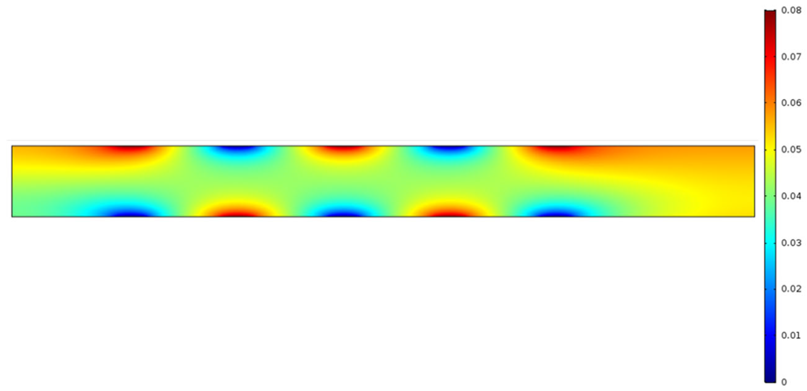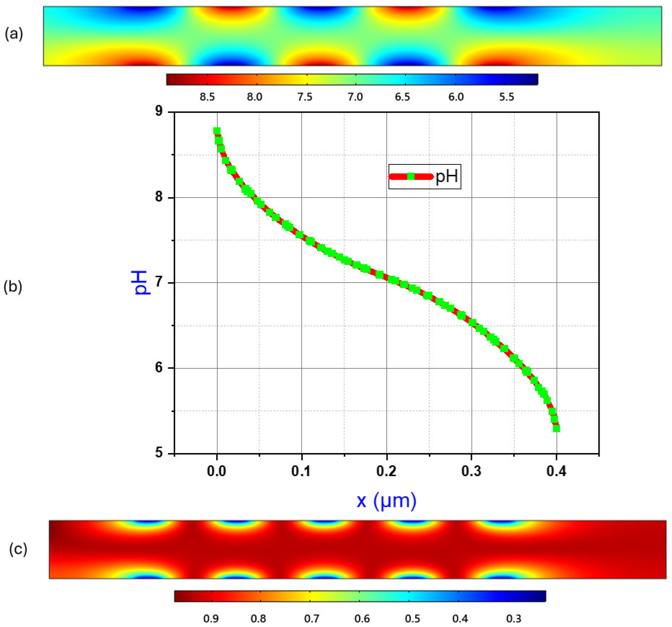Figure 4a demonstrates the pH-gradient of the aqueous solution in the micro-channel in presence of an electrolyte, such as NaCl. The simulation clearly demonstrates that, under an applied electric field, for an aqueous electrolytic solution, the anode is acidic in nature (low pH; blue region), the cathode is basic in nature (high pH; red region), and there is a continuous gradient of pH that exists between each pair of electrodes, showing mostly neutral pH (green region) around the central part of the micro-channel. Figure 4b supports the observation quantitatively.

The line graph in Figure 4b plots measured pH values from the same simulation on the y axis with distance from the bottom of the channel plotted on the x axis. The coordinates (0.6 µm, 0.0 µm) and (0.6 µm, 0.4 µm) are used to plot a 2D cut line. Figure 4b represents a cross section of the microchannel in this way as means to understand how pH gradients are created between anode and cathode across the channel. For both Figure 4a,b, the highest pH reading is 8.78 and the lowest pH is 5.29. Recall that the microchannels in this experiment are a height of 0.4 μm.

3.4. Conductivity of Microchannel

Next, we tested the conductivity of the empty microchannel. Figure 4c shows a surface graphic where the greatest conductivity is found at locations furthest from both anode and cathode. These central locations see a conductivity of 1 S/m as indicated by a deep red corresponding to the graphical color legend to the right of the surface graphic in Figure 4c. Note how a distinct semi-circular gradient of decreasing conductivity defines each electrode location at the top and bottom of the microchannel. Distinct rounded bands of roughly 0.7 S/m and 0.6 S/m surround silvers of 0 S/m.

The simplest explanation, from the electro-chemistry point of view, of this conductivity difference is that, most probably, the anions and cations in the electrolytic solution can move freely at locations furthest from both electrodes, i.e., at the center of the microchannel, making a pure water conductive in the presence of a given electrolyte.

3.5. Electrolytic Fluid

The surface graphic in Figure 5 shows the electric potential of the electrolytic fluid used to model all experiments in this study. All proteins in this study were suspended in an electrolytic solution of NaCl. We note that the potential of the fluid here shows a potential very similar to that of the channel from Figure 3, but with notably smaller transitional regions toward the median charge potential (~0.04 V). The electric potential of the fluid instead displays much tighter regions of 0.08 V at anode and 0 V at cathode with a larger region of ~0.04 V in the remainder of the channel.

3.6. Weak Acid and Base Surface Concentration Behavior

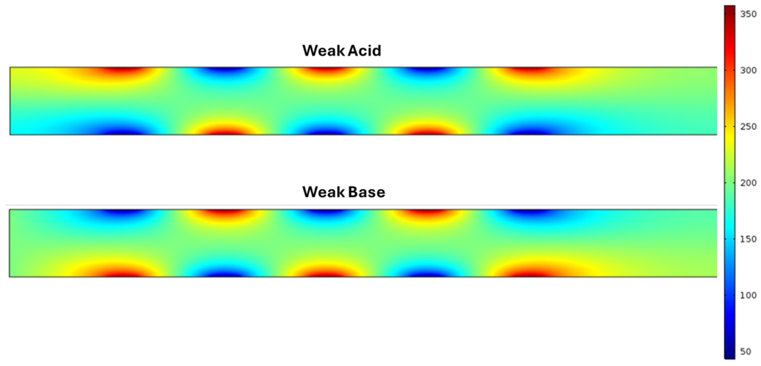
Next, we simulated a weak acid and weak base in the microchannel at the electrode array under the same conditions as previous simulations with 0.08 V of AC applied at the anode. Figure 6 shows a surface graphic of Weak Acid (top). We recorded a maximum concentration of 375.24 mol/m³ at the anode, and a notable region of low concentration is focused on the cathode. The regions of high and low concentration in these trials demonstrate the same semi-circular shape seen in previous trials at varying degrees. The surface graphic for Weak Base in Figure 6 (bottom) shows an identical but inverse behavior at the anode and cathode sides of the electrode array. 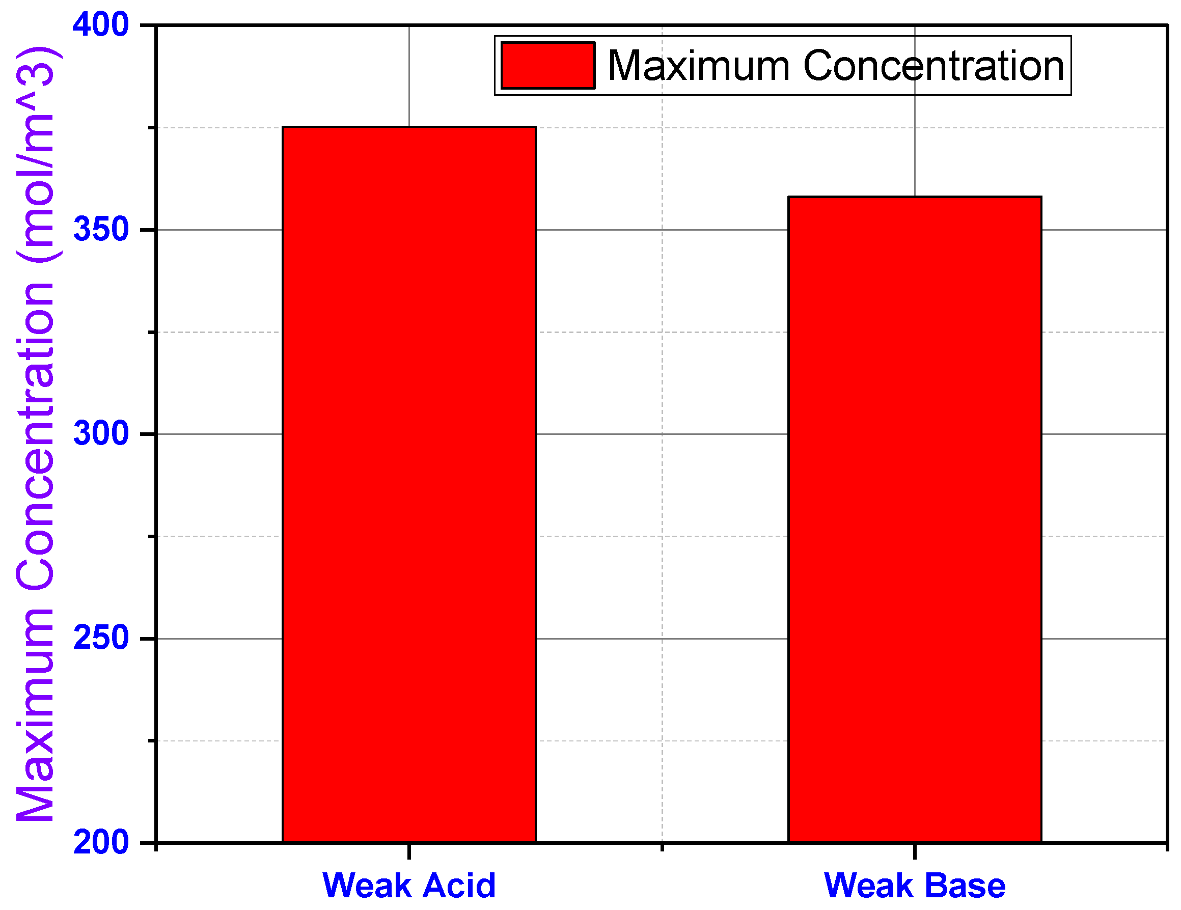Here, the simulation of weak base under the same conditions results in the maximum concentration of 358.06 mol/m³ occurring at the cathodes with the lowest concentration occurring at the anode. The bar graph in Figure 7 shows the maximum concentrations of each simulation visualized in Figure 6. These simulations demonstrate how the pH of a solution dictates the distribution of concentration in a fluid within a microchannel in the presence of AC.

From an electrochemical point of view, a most likely explanation of the behavior of weak acid and weak base in the microchannel is the following. Unlike the electrolytes, the weak acids and bases mostly remain undissociated in aqueous solution. While dissociated, the conjugate anion of a weak acid behaves as a strong base, and the conjugate cation of a weak base behaves as a strong acid. In the presence of electrolytic ions, the conjugated base and conjugated acid forms a ‘buffer solution’ with the corresponding weak acid and weak base, respectively. When the buffer solution is in the presence of a certain excess proton concentration, i.e., at a low pH, the conjugate anion of the dissociated weak acid immediately consumes H⁺, driving the equilibrium towards undissociated weak acid. Similarly, an abundance of hydroxyl (OH⁻) ions or lack of H⁺ concentration at certain threshold, i.e., at a high pH, a weak base is forced to remain mostly undissociated. Following is the chemical equilibrium of a hypothetical weak acid (HA) and a weak base (BOH), respectively, in an aqueous solution of electrolyte.

Weak Acid at low pH: HA (aq.) + H₂O (aq.) + Na⁺(aq.) ← Na⁺ (aq.) + A⁻ (aq.) + H₃O⁺ (aq.)

(13)

Weak Base at high pH: BOH (aq.) + Cl⁻ (aq.) ← B⁺ (aq.) + Cl⁻ (aq.) + OH⁻ (aq.)

(14)

Equations (13) and (14) represent the drive of the equilibrium of a weak acid and its conjugate salt form in presence of excess H⁺ and a weak base and its conjugate salt in presence of excess OH⁻. Consequently, under an electric field, the weak acid dissociation around the anode is less favored due to the acidic condition (see Equation (13); low pH). Most likely, the half reactions at both of electrodes in presence of a weakly acidic buffer solution are the following:

Weak Acid:

Cathode (weak acid) with E = 0 V: 4H₃O⁺ + 4e⁻ → 4OH⁻ (aq.) + 2H₂ (g)

(15)

At high pH: HA (aq.) + OH⁻ (aq.) → A⁻ (aq.) + H₂O (aq.)

(16)

Anode (weak acid) with E = 0.08V: 2H₂O (aq.) → 4H⁺ (aq.) + O₂ (g) + 4e⁻

(17)

At low pH: HA (aq.) + H₂O (aq.) ← A⁻ (aq.) + H₃O⁺ (aq.)

(18)

At solution: NaCl (aq.) → Na⁺ (aq.) + Cl⁻ (aq.)

(19)

Equations (15)–(18) show that, at the cathode, the presence of an excess of OH⁻ accelerates the dissociation of the weak acid (HA) to its conjugate base (A⁻), driving the electric flow in between the electrodes through the ion-transport of A⁻ within the electrolytic solution. At anode, the excess of H⁺ is quickly removed by the A⁻ ions and accumulates as HA around the anode, thus completing the circuit.

Conversely, due to the basic environment around the cathode (see Equation (16); high pH), the dissociation of a weak base is suppressed. The likely half reactions at the electrodes are the following in the presence of a weak base:

Weak Base:

At low pH: BOH (aq.) + H₂O (aq.) → B⁺ (aq.) + OH⁻ (aq.) + H₂O (aq.)

(20)

Anode (weak base) with E = 0.08 V: 4OH⁻ (aq.) → 2H₂O (aq.) + O₂ (g) + 4e⁻

(21)

Cathode (weak base) with E = 0 V: 4H₂O (aq.) + 4e⁻ → 4OH⁻ (aq.) + 2H₂ (g)

(22)

At high pH: BOH (aq.) + H₂O (aq.) ← B⁺(aq.) + OH⁻ (aq.) + H₂O (aq.)

(23)

At solution: NaCl (aq.) → Na⁺ (aq.) + Cl⁻ (aq.)

(24)

Equations (20)–(23) show that the low pH around the anode favors a weak base (BOH) to be dissociated into its strong conjugate acid (B⁺), which transport the charges to cathode through the electrolytic solution and removes the accumulated OH⁻ at the electrode. Thus, the electric circuit becomes complete by the surface accumulation of the weak base around the cathode. Figure 8 illustrates that the simulation agrees that the surface concentration of the weak acid is largely concentrated around the anode and the weak base around the cathode.

By definition, the pK_a (=−log₁₀K_a) is the measure of the strength of an acid or base based on their dissociation rate. A pK_a of an acid and the pH = −log₁₀C_H+ is related as following:

Hydrolysis of a weak acid: HA (aq.) + H₂O (aq.) ⇌ A⁻ (aq.) + H₃O⁺ (aq.)

(25)

Dissociation Constant of the weak acid: K_a = (C_H⁺. C_A⁻)/C_HA

(26)

Henderson-Hasselbach Equation: pK_a = pH − log₁₀ (C_A⁻/C_HA)

(27)

pK_a is the inherent property of a weak acid/base specifying their ability to donate or accept H⁺. A low pK_a for an acid indicates high donation of protons, leading to a low pH medium. However, in an aqueous solution, as the dissociation strength of water (pK_w) is 14, the dissociation rate of a weak base (pK_b) in an aqueous solution is related to pH and pK_a in the following manner:

Hydrolysis of a weak base: BOH (aq.) + H₂O (aq.) ⇌ B⁺ (aq.) + OH⁻(aq.) + H₂O (aq.)

(28)

Dissociation Constant of the weak base: K_b = (C_B⁺. C_OH⁻)/C_BOH

(29)

$$\begin{array}{l}\mathrm{Relation} \text{of} {\mathrm{pK}}_{\mathrm{b}} \mathrm{with} {\mathrm{pK}}_{\mathrm{a}}\mathrm{and} \mathrm{pH} \mathrm{in} \mathrm{an} \mathrm{aqueous} \mathrm{solution}:\\ {\mathrm{pK}}_{\mathrm{b}}=-{\log }_{10}{\mathrm{C}}_{{\mathrm{OH}}^{-}}-{\log }_{10}({\mathrm{C}}_{{\mathrm{B}}^{+}}/{\mathrm{C}}_{\mathrm{BOH}})\\ =14 + {\log }_{10}{\mathrm{C}}_{{\mathrm{H}}^{+}}-{\log }_{10}({\mathrm{C}}_{{\mathrm{B}}^{+}}/{\mathrm{C}}_{\mathrm{BOH}})\\ =14 - \mathrm{pH} + {\log }_{10}({\mathrm{C}}_{\mathrm{BOH}}/{\mathrm{C}}_{{\mathrm{B}}^{+}})\\ \approx 14-{\mathrm{pK}}_{\mathrm{a}}\end{array}$$

(30)

A low pK_b indicates strong dissociation of the corresponding base. The pK_a (=8) of the given aqueous solution of the weak acid and the pK_b (=14 − pK_a = 14 − 6 = 8) of the given aqueous solution of the weak base (given pK_a = 6) indicate that similar dissociation rates. In the presence of an electrolyte, the solution of both weak acid and base generates a mixture of buffer solution having a pH slightly less than 7.0. As a result, the accumulation of a weak acid at the anode is slightly higher than the accumulation of a weak base at the cathode, as evidently shown in Figure 7.

A protein, in general, is comprised of various amino acids having multiple functional groups that can accept or donate protons based on the pH of the aqueous solution, if soluble in water. Hence, depending on the total pH of the solution, a protein can have either a net negative or a positive charge, behaving as a zwitterion. Having a net positive charge, a protein can act as an acid or having a net negative charge, a protein can act as a base. Therefore the protein solutions, may behave as a weak acid or weak base respectively, based on the dissociation strength of the proteins. However, at certain pK_a range, the same protein solution may not have any negative or positive charge, which is otherwise known as ‘isoelectric point (pI)’. Hence, for a solution of multiple proteins, at a certain pH of the solution; if the pH > pI of a given protein in the solution, then the protein has a net negative charge in the solution; otherwise, if the pH < pI of the protein, then in the solution the protein remains positively charged. Therefore, under an applied electric field, the protein solution having pI less than the overall pH accumulates at the anode and solution having pI greater than the overall pH accumulates at the cathode within the microchannel. Utilizing this property of protein in the presence of a buffer, and under a certain potential difference between the electrodes, the simulations are run within the microchannel for a mixture of five hypothetical proteins, having various pI values, in the presence of a buffer solution.

3.7. Protein Molar Concentrations

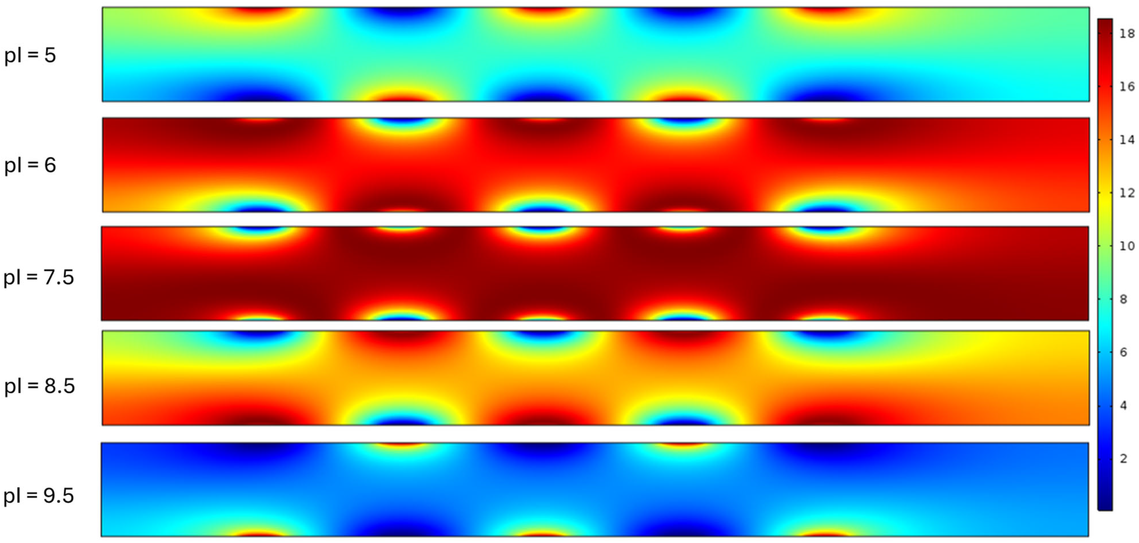
A constant 0.08 V of AC was simulated at the electrode array for the protein solutions 1 through 5, having pI = 5.0, 6.0, 7.5, 8.5, and 9.5 respectively. Diffusivity for all proteins was set at 5 × 10⁻¹⁰ m/s² with an inlet concentration of 5 mM. Our results show that the 5 protein solutions demonstrated notably different behavior in the distribution of molar concentration. Figure 8 shows a compilation of graphical renderings describing recorded surface concentration in the microchannel at the array. Since numerical concentration results varied between experiments, color coding in this graphic is relative with extremes described between ‘high’ and ‘0’. Channel height is measured in μm from the bottom of the microchannel (0 μm) to the top of the microchannel (0.4 μm). All five proteins in the study have different pH.

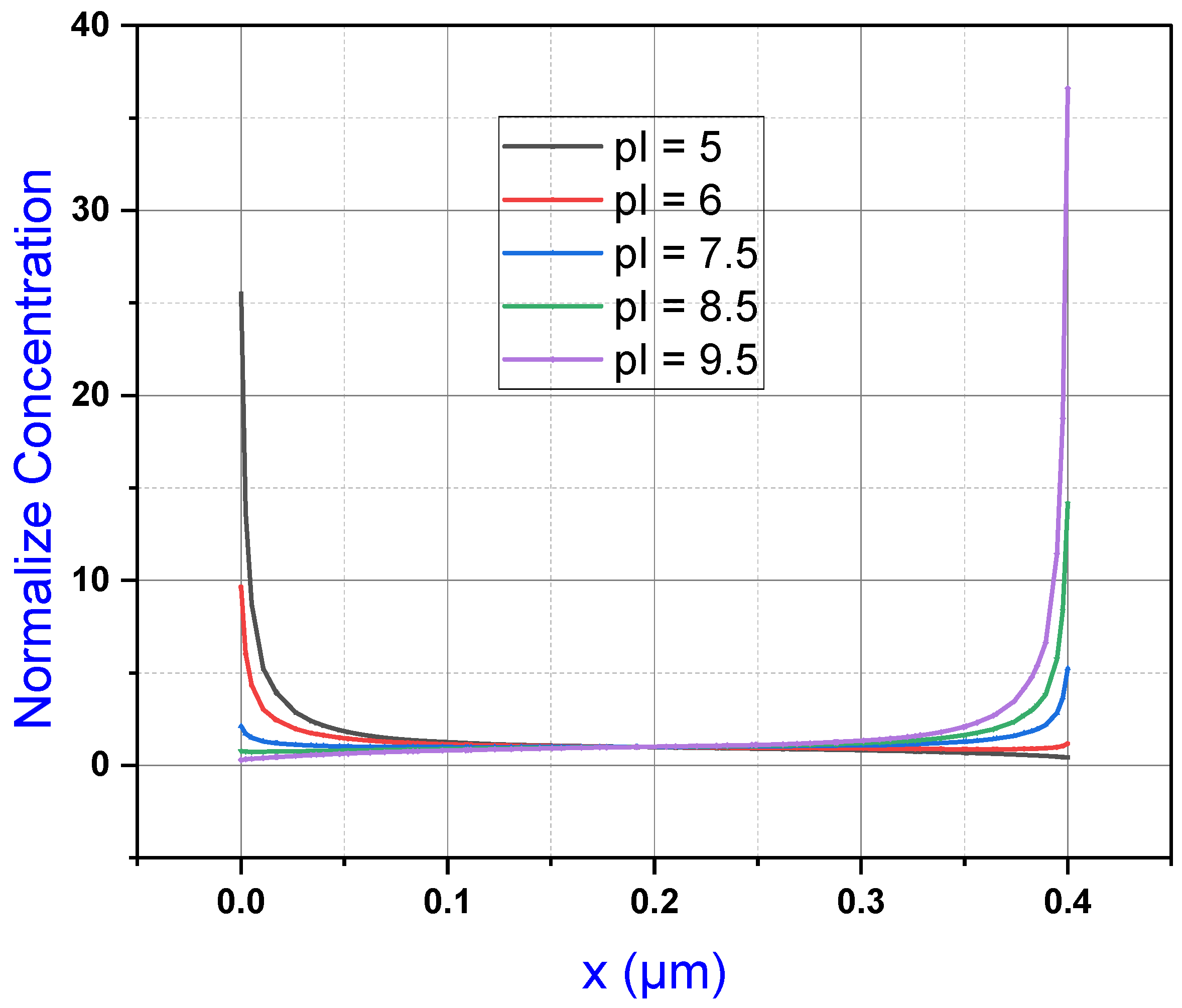
In the protein 1 (pI = 5.0) solution we see the greatest molar concentration of 11.72 mol/m³ at the site of positive charge. Concentration decreases moving vertically across the channel toward the cathode where concentration is effectively 0, or 0.209 mol/m³. Referring to Figure 9, we see that all five protein solution concentrations visualized in Figure 8 are superimposed on one another. Note that the scope of the graph in Figure 9 consists of molar concentration (mol/m³) on the y-axis and the distance vertically across the microchannel from the bottom of the channel to the top. Locating protein 1 on this graph represented by the dark blue line, we can see the how the concentration of the solution arcs in a negative parabolic curve from 0.209 mol/m³ toward a concentration of roughly 5 mol/m³, recorded as 4.99 mol/m³ at 0.17 μm. From this point, the parabolic curve changes to a positive parabolic curve up to the maximum concentration for protein 1 at 11.72 mol/m³.

The graphic of the protein 2 (pI = 6.0) solution from Figure 8 shows an orientation of concentration like that of protein 1 with high concentration at the anode and low concentration at the cathode, but with a much different distribution. Here, we can see that the high concentration of 5.71 mol/m³ gathers around the anode. This high concentration is located at height of 0.34 from the bottom of the channel with a small region of lower concentration of 3.95 mol/m³ at 0.4 μm. Concentration remains relatively high moving toward the cathode. Concentration is 4.92 at the 0.17 μm midpoint of the channel as can be seen in Figure 9. Following the orange line for protein 2, we see how this concentration gradient takes on a more linear relationship down toward the cathode until 0.064 μm where it begins to decline at a parabolic rate down to 0.67 mol/m³ at 0 μm. The visualization of protein 2 in Figure 8 expresses this increased rate of change by the tighter regions of decreasing concentrations.

Protein 3 (pI = 7.5) mimics the drops in concentration at the electrodes as seen in protein 2 but does so more abruptly. We can also note that the high concentrations occurred in the middle of the microchannel and were between 0.03 μm and 0.34 μm. The concentration in the protein 3 simulation does not drop below 4 mol/m³. Figure 9 gives a clear visualization of this restricted distribution as the gray line for protein 3 is a more horizontal line contained within a more neutral pH region. Protein 3 shares the point of equal concentrations, as do other solutions at 0.17 μm in the microchannel where its concentration is 4.91 mol/m³. Points of low concentration occur at each electrode with 0.75 mol/m³ at a height of 0 μm with the cathode and 1.02 mol/m³ at 0.4 μm with the anode.

Protein 4 (pI = 8.5) demonstrated notable regions of low concentration at the anodes. Here, the low was measured at 0.25 mol/m³ at 0.4 where the anode is located. The highest pH value occurred at the cathode with a concentration of 9.53 mol/m³ at a height of 0 μm. The surface graphic in Figure 8 for protein 4 displays regions of semicircular high and low regions at the respective electrodes. Concentration declines moving toward the center of the microchannel, giving way to a large region of lower concentration where 6.89 mol/m³ was recorded at a height of 0.17 μm. In Figure 9, we can see this decline in concentration for protein 4 as indicated by the yellow line mimicking a parabolic rate moving from the cathode at 0 toward the 0.17 midpoint where the line then assumes a negative parabolic-like arc toward the lowest concentration at 0.4 μm.

Protein 5 (pI = 9.5) demonstrated unique behavior at the electrode array where most of the concentration was focused on the cathode at 0 μm with a recorded high of 18.58 mol/m³. The surface graphic in Figure 8 indicates this sudden elevation in concentration with very small semicircles of high concentration at cathode sites, which quickly give way to a large region of much lower concentration across the channel to the anode at 0.4 μm. The graph in Figure 9 gives a clearer indication of this dramatic distribution of concentration, as indicated by the light blue line for protein 5. Here, we can see the dramatic parabolic drop in concentration from 18.58 mol/m³ at a height of 0 μm to the shared midpoint where concentration was measured at 5.03 mol/m³ at 0.17 μm. Like other simulations, the concentration readings within the mid-channel region, around 0.17 μm, demonstrate a much gentler gradient. From here, the curve takes on a notably more gradual negative parabolic arc toward a measured concentration of 0.11 mol/m³ at 0.4 μm.

Here, in the presence of a buffer solution, having a pH slightly less than 7.0, the protein solutions accumulate at cathode or anode depending on their corresponding pI values and how they deviate from the overall pH of the solution. Depending on the predominant net charge on the protein, the plausible half-reactions are very similar to the cases of weak acids and weak bases at the electrodes. A protein with a net negative or positive charge (Pr⁻ or PrH₂⁺) equilibrates with the net neutral protein molecule (HPr) in the buffer solution having electrolytes.

If pH > pI, the protein solution is negatively charged in the presence of a buffer:

HPr (aq.) + H₂O (aq.) ⇌ Pr⁻ (aq.) + H₃O⁺ (aq.)

(31)

NaCl (aq.) → Na⁺ (aq.) + Cl⁻ (aq.)

(32)

If pH < pI, the protein solution is positively charged in the presence of a buffer:

HPr (aq.) + H⁺ ⇌ PrH₂⁺ (aq.)

(33)

NaCl (aq.) → Na⁺ (aq.) + Cl⁻ (aq.)

(34)

However, the difference between the pI and the overall pH of the solution dictates the dissociation equilibrium of a protein in the solution; hence, it guides the accumulation of protein at corresponding electrodes. As a result, the distribution of the concentration of a given protein solution along the microchannel and at the electrode surfaces, as quantitatively shown in molar concentrations in Figure 9, can primarily be estimated from simulation results shown in Figure 8. The higher concentration of protein at cathode indicates more positively charged proteins from the solution are discharged near the electrode (Protein 5 > Protein 4 > Protein 3). At anode, such accumulation indicates more negatively charged protein are discharged from the solution (Protein 1 > Protein 2). However, Protein 2 and Protein 3 rather have a uniform distribution in between the electrodes and minimal accumulation around the anode and cathode surface, respectively, indicating a small quantity of negatively charged and positively charged proteins are generated, respectively, as their pI is closer to the overall pH. For other three cases, the overall pH is either far less or far greater than their pI s; hence, depending on the deviation of pI from the overall pH, given proteins are found to be more concentrated around the corresponding electrode surface. These estimations can be validated from the simulation, by measuring the surface concentration of a given protein in the solution and at the electrodes.

Anode reaction for a protein solution having pH > pI:

Anode with E = 0.08 V: 2H₂O (aq.) → 4H⁺ (aq.) + O₂ (g) + 4e⁻

(35)

Pr⁻ (aq.) + H⁺ (aq.) → HPr (aq.)

(36)

Cathode reaction for a protein solution having pH < pI:

Cathode with E = 0 V: 4H₂O (aq.) + 4e⁻ → 4OH⁻ (aq.) + 2H₂ (g)

(37)

PrH₂⁺ (aq.) + OH⁻ (aq.) → HPr (aq.) + H₂O (aq.)

(38)

Therefore, the fundamental goal of these simulations is whether a given protein solution, based on its corresponding pI, can be identified and separated in a micro-channel by tuning the overall pH using buffer solutions. Dense accumulation of protein around the cathode or anode surface indicates a relatively high concentration of negatively charged or positively charged proteins are generated in the solution, indicating pIs far from the overall pH of the solution and behave as a relatively stronger base or acid, respectively. For Protein 1 (pI = 5.0), as evident from Figure 8, the accumulation around the anode in a denser concentration identifies the protein solution was mostly negatively charged in the solution, as shown in Equation (36). Protein 1 generates the conjugate base in the solution, transported to anode and accumulated around the surface of the anode according to Poisson and Nerst–Plank equations. Protein 2, having pI (=6.0) closer to overall pH of the solution, is dissociated in a lower amount of negatively charged protein in the solution and deposited in a lesser amount around the anode surface. A rather uniform spread of protein distribution from the middle of the micro-channel up to around the anode, as seen in Figure 8, supports the inference. In case of Protein 3–5, as seen in Figure 8, there is an inverse trend of accumulations around the electrodes, clearly indicating that they were mostly dissociated as a cation in the solution, and a dense accumulation around cathode indicates higher pI than the overall pH of the solution. Protein 3 (pI = 7.5) solution shows a uniform spread of protein concentration along the micro-channel up to the anode, indicating the protein weakly dissociated into its’ positively charged counter ion (see Equation (38)) and rest is mostly undissociated along the microchannel. Protein 4 with pI = 8.5 is dissociated more in cations compared to Protein 3 in the solution, hence comparatively higher accumulation of the protein at the cathode and less concentration of protein in solution is observed within the microchannel. Protein 5, having pI = 9.5, as also evident from Figure 8, mostly ionizes into cationic counterpart and mostly deposited around the cathode. In this case, the protein leaves almost no trace in the solution in between the microchannel, rather found as a thick deposition around the cathode.

The distribution of the concentration of the corresponding protein solution along the microchannel and at the electrode surfaces is quantitatively shown in molar concentrations in Figure 9. It supports the simulation results shown in Figure 8. The concentration of Protein 1 (pI = 5.0) is highest at the anode followed by Protein 2 (pI = 6.5) and almost zero around the cathode, indicating both proteins were predominantly negatively charged in the solution. On the other hand, Protein 5 (pI = 9.5) has the highest concentration around cathode, followed by Protein 4 (pI = 8.5) and Protein 3 (pI = 7.5), and almost no trace is found around the anode, indicating these proteins were predominantly cationic in the solution. As discussed, this is due to the differences between pI of the individual proteins and overall pH of the solution. Protein 3 (pI = 7.5), being very close to the pH of the buffer solution, was found to have minimal accumulation around the cathode. With the change of anode voltage from 0.02 V to 0.14 V, the qualitative features of the accumulation of protein solutions around the electrodes remain same; however, the accumulation becomes significant for each protein solution with the increase in the anode voltage (see surface figure comparison shown in Figures S2–S4 in the Supplementary Information).

3.8. Isoelectric Point

Despite how individual proteins react to simulated conditions at the electrode array or their maximum recorded molar concentration, the superimposed line graphs of proteins 1 through 5, in Figure 9, reveals a shared point of concentration mid-channel at roughly 0.17 μm. This convergence of concentrations reveals the isoelectric point in the protein solutions where molecules hold no electrical charge. Isoelectric separation is occurring via electrophoresis at this point in the channel between the anodes and cathodes in the array. Around the middle of the microchannel (0.2 μm), all the ions from the dissociation of electrolyte, weak acid and weak base buffer, and proteins stay in equilibrium and move freely within any direction of the microchannel, helping an efficient ion transport within the microchannel. Hence, all the proteins have the same concentration around the mid region of the microchannel.

We can make an important observation about the relationship between protein pH and concentration behavior at the electrode array here. We can see that proteins 1 and 2 exhibit similar overall behavior with higher concentrations at anode while lower concentrations occur at cathode. The fact that each of these proteins with different pH values share a common point mid-channel, as shown in Figure 9, indicates as shared neutrality in molecular charge where isoelectric separation will occur for all proteins in the study, regardless of maximum concentration. It can also be understood by looking at the behavior of the lines in the Figure 9 graph that higher maximum concentrations lead to more dramatic parabolic curves at the electrodes. Solutions with lower maximum pH values display a more linear distribution of concentration across the channel with only slightly parabolic trends at the electrodes.

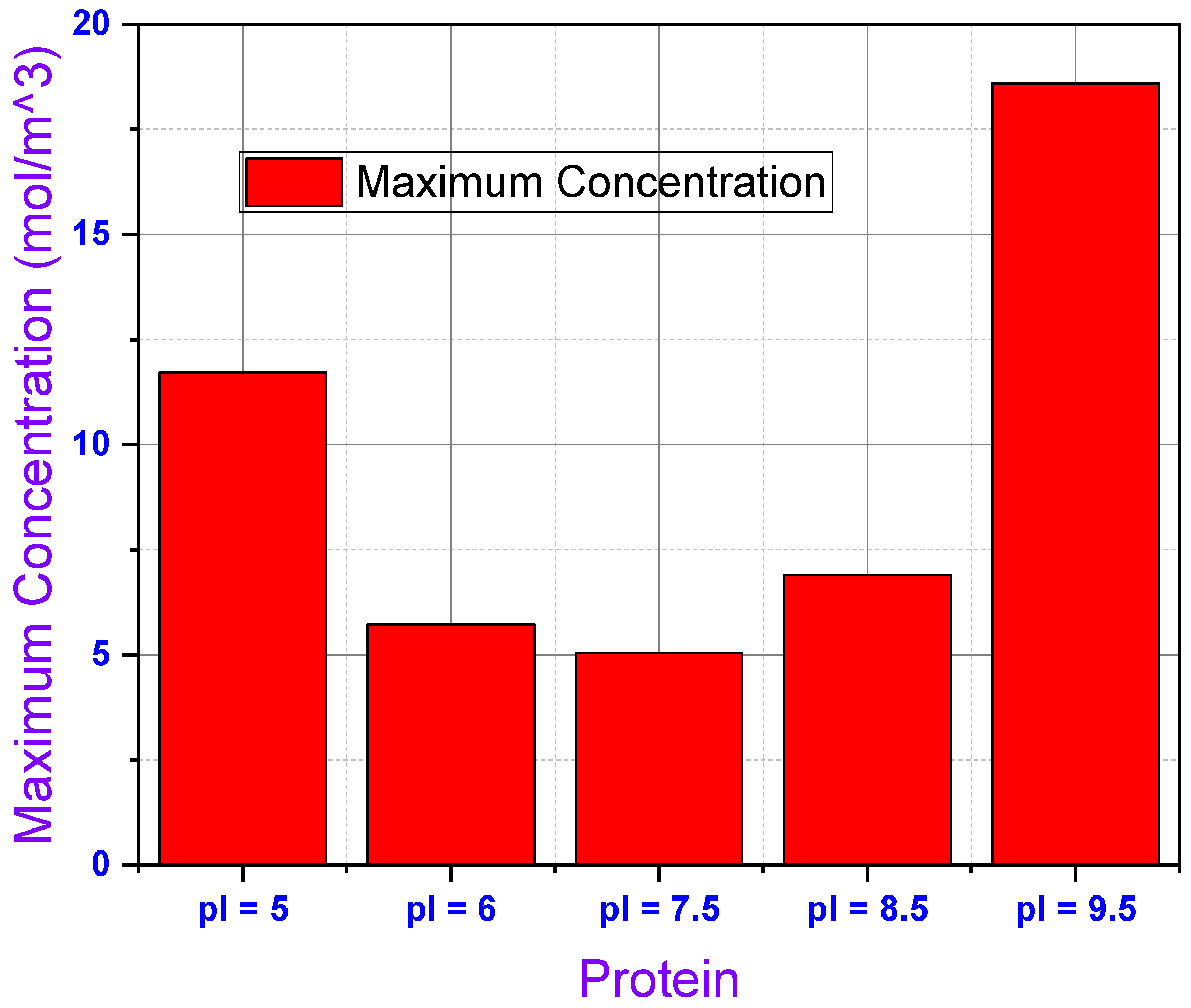
Lastly, Figure 10 provides an estimate of the surface concentration of proteins at corresponding electrodes and the microchannel in terms of a bar graph of maximum molar concentrations recorded anywhere in the microchannel for the five proteins in this study. This graph highlights the different capacities for surface concentration for the five proteins studied in this simulation. We can see that Protein 1 had the second highest concentration recorded in the microchannel at 11.29 mol/m³. Protein 2 and 3 had similar maximum concentrations at 5.67 mol/m³ and 5.04 mol/m³, respectively, with Protein 3 returning the lowest recorded maximum concentration for the experiment. Protein 4 showed the third highest concentration at 6.75 mol/m³ and Protein 5 had the highest recorded concentration of the experiment at 17.01 mol/m³. As the difference between the pI and overall pH of the solution dictates the strength of dissociation of proteins into their anionic/cationic counterparts, Protein 1 and Protein 5 show maximum accumulation due to a large disparity between their corresponding pI and pH of the solution. On the other hand, Protein 2, Protein 3, and Protein 4 show accumulation at almost similar concentration due to small differences between their pI and the overall pH of the solution. Protein 3 has the closest pI with respect to the pH of the solution, hence, the accumulation of this protein at the surface is the minimum.

4. Discussion

The targeted separation or mixing of diverse protein solution(s) via EOF principle depends on the intrinsic isoelectric point (pI) of the protein(s) in aqueous solutions. The presence of an electrolyte in an aqueous solution facilitates ion transport as well as provides a ground of electrochemical reactions to perform by making the surroundings of the cathode basic and the anode acidic. Plus, in the presence of a buffer, as a mixture of weak acid and its conjugate base, or of weak base and its conjugate acid, or in presence of both weak acid and base, the pH of the solution can be tuned. A given protein solution in presence of such buffer, if it has pI less than pH of the solution, then mostly dissociate into negatively charged ions and if it has pI more than the pH of the solution, then it mostly dissociates into positively charged ions. Hence, an accumulation is observed at anode or cathode depending on this difference between pI and the pH of the solution. Moreover, the extent of such accumulation of the protein depends on how much further away the corresponding pI is from the overall pH of the solution. More the deviation, a tighter accumulation of the protein is observed around the corresponding electrode, and lesser differences between pI of the protein and the pH of the solution are reflected in more disperse accumulation around the electrodes and along the microchannel. Through other factors, such as the size of the protein ions, presence of multiple polar functionals within the protein, the zeta potential generated near the electrode surfaces, dielectric constants and viscosity associated with a particular aqueous protein solution, and voltage gradient/strength of the electric field, may also play a significant role in the qualitative/quantitative surface accumulation; however, our simulations candidly demonstrate that the pI of a protein and a choice of an appropriate buffer can delegate the surface accumulation of the protein towards a desired electrode as well as control the concentration of surface accumulation. Hence, this proposition can make a significant contribution towards accurate identification and separation of protein solutions without much sample loss within the microchannels using the EOF principle.

The findings on charge-based separation methods in proteomics reveal significant advantages, such as potential label-free specificity in limited workflow contexts with the potential to preserve protein structure and function, high resolution for separating proteins differing by 0.1 pH units in under a minute, and low sample consumption due to nanoliter-scale operations. The hypothetical device’s flexibility allows for easy reconfiguration through simple buffer pH adjustments. These advancements can enable novel applications like selective capture of disease-specific exosomes for early biomarker discovery, post-translational modification profiling through direct coupling to mass spectrometry, rapid concentration of virus-like particles for vaccines, and enhanced real-time studies with organ-on-chip technology. Additionally, parallel fractionation of therapeutic antibody variants accelerates lead identification while maintaining binding affinity.

Additionally, within the scope of our work, we would also like to highlight recent progress of relevance through additional works applicable to microfluidic protein separation: Peng et al. (2023), Yang et al. (2024), and Jacquat et al. (2023) [36,37,38]. To start, Peng et al. (2023) created an automated DMF chip that integrates reduction, alkylation, digestion, isotopic labeling, and HPLC-MS/MS for nanogram-scale proteomics, an approach readily extendable to spatial proteomics via patterned droplet printing [36]. Yang et al. (2024) developed an active-matrix droplet microfluidics system (AM-DMF-SCP) that isolates, lyses, digests, and purifies single cells in nanoliter droplets before DIA-MS, identifying over 2200 proteins per HeLa cell in 15 min and making it amenable to immunoaffinity enrichment for the analysis of circulating tumor cells [37]. Jacquat et al. (2023) introduced nanocavity diffusional sizing (NDS), utilizing PDMS–silica nanocavities and single-molecule fluorescence, to extract protein hydrodynamic radii without the need for labels [38]. This approach can be paired with micro dialysis for real-time monitoring of biomarkers and physiological parameters [38]. Together, our work and platforms enable the possibility of rapid, high-sensitivity, low-volume, yet scalable protein assays that amplify efforts in early diagnostics and personalized medicine. Future work may fuse AI-driven analysis and multimodal sensing into these chips. Such integrations could redefine predictive diagnostics and continuous health monitoring.

5. Conclusions

Together, these results demonstrate that pH-driven modulation of protein net charge achieved by setting buffer pH at, just above, or below each protein’s isoelectric point can be leveraged in a simple electrode array to steer and capture target molecules programmatically. At pH = pI, a protein carries no net charge and remains stationary; offsetting the pH induces a predictable electrophoretic drive toward a chosen electrode, enabling precise, label-free transport and immobilization without complex device geometries. Through modifying experimental parameters, microfluidic setups can become better suited at differentiating or concentrating proteins, based on the iso-electric point of protein and pH environment in the solution and around the electrodes, to optimize biochemical investigations. The simulation results underpin the fact that by varying the pH of a protein solution using a desired buffer of weak acid/weak base in a microchannel, proteins can be directed to accumulate at a chosen electrode with a desired concentration. Hence, an efficient protein separation within micro-channels can be achieved with minimal loss of the sample and this technique can be proven widely useful and cost-effective for biomedical and biochemical separations. The data support and illustrate a strong dependency between rapid electrode polarity shifts and the fluid’s behavior in the channel. By co-optimizing buffer pH relative to the isoelectric point, DC field parameters (voltage), and bulk flow rate, one can generate distinct migration profiles for different proteins. Small pH offsets (±0.1 pH units) yield gentle, broad capture zones for proteins with low net charge, while larger offsets (±0.3 pH units) and higher field amplitudes accelerate strongly charged species into tight, high-resolution bands at specific electrodes. Fine-tuning the flow rate adjusts residence time so that proteins differing in size, charge density, or hydrodynamic drag travel along separate paths, demonstrating the adaptability of this method. This combination of pH control and field tuning transforms a straightforward microchannel with planar electrodes into a versatile, label-free separation and enrichment platform for a wide range of complex protein mixtures.

References

1. Kaniansky, D.; Masár, M.; Bodor, R.; Žúborová, M.; Ölvecká, E.; Jöhnck, M.; Stanislawski, B. Electrophoretic separations on chips with hydrodynamically closed separation systems. Electrophoresis 2003, 24, 2208–2227. [Google Scholar] [CrossRef]
2. Huang, Y.F.; Huang, C.C.; Hu, C.C.; Chang, H.T. Capillary electrophoresis–based separation techniques for the analysis of proteins. Electrophoresis 2006, 27, 3503–3522. [Google Scholar] [CrossRef]
3. Mei, L.; Cui, D.; Shen, J.; Dutta, D.; Brown, W.; Zhang, L.; Dabipi, I.K. Electroosmotic mixing of non-Newtonian fluid in a microchannel with obstacles and zeta potential heterogeneity. Micromachines 2021, 12, 431. [Google Scholar] [CrossRef]
4. Dutta, D.; Smith, K.; Palmer, X. Long-range ACEO phenomena in microfluidic channels. Surfaces 2023, 6, 145–163. [Google Scholar] [CrossRef]
5. Dutta, D.; Palmer, X.; Lim, J.Y.; Chandra, S. Simulation on the separation of breast cancer cells within a dual-patterned end microfluidic device. Fluids 2024, 9, 123. [Google Scholar] [CrossRef]
6. Han, W.; Li, W.; Zhang, H. A comprehensive review on the fundamental principles, innovative designs, and multidisciplinary applications of micromixers. Phys. Fluids 2024, 36, 101306. [Google Scholar] [CrossRef]
7. Bigio, J.; van Gemert, W.; Kaiser, B.; Waning, B.; Pai, M. Asia emerges as a hotbed of diagnostic innovations for tuberculosis. J. Clin. Tuberc. Other Mycobact. Dis. 2021, 25, 100267. [Google Scholar] [CrossRef] [PubMed]
8. Sultana, T.A.; Rahman, M.M.; Rahim, R.; Nasir, T.A.; Sultana, G.S.; Alam, M.S.; Hasan, R. Molecular diagnostic tests in Bangladesh: Opportunities and challenges. Pulse 2016, 8, 51–61. [Google Scholar] [CrossRef]
9. Digital Diagnostics for Africa Network. The potential of digital molecular diagnostics for infectious diseases in sub-Saharan Africa. PLoS Digit. Health 2022, 1, e0000064. [Google Scholar]
10. Wijekoon, N.; Gonawala, L.; Ratnayake, P.; Liyanage, R.; Amaratunga, D.; Hathout, Y.; Steinbusch, H.W.; Dalal, A.; Hoffman, E.P.; de Silva, K.R.D. Molecular diagnostics of dystrophinopathies in Sri Lanka towards phenotype predictions: An insight from a South Asian resource-limited setting. Eur. J. Med. Res. 2024, 29, 37. [Google Scholar] [CrossRef]
11. Hossain, F.; Ghosh, P.; Chowdhury, F.R.; Basher, A.; Ahsan, H.M.N.; Khan, A.H.; Shumu, S.J.; Jahan, T.; Roy, C.K.; Arefin, A.N.; et al. Evaluating a rapid molecular assay in a mobile laboratory for improved diagnosis of dengue in Bangladesh. Int. J. Infect. Dis. 2025, 150, 107299. [Google Scholar] [CrossRef]
12. Cain, D.; Cao, E.; Vlassiouk, I.; Schäffer, T.E.; Siwy, Z.S. Ion concentration polarization causes a nearly pore-length-independent conductance of nanopores. Faraday Discuss. 2024, 257, 344–359. [Google Scholar] [CrossRef]
13. Chircov, C.; Grumezescu, A.M. Microelectromechanical systems (MEMS) for biomedical applications. Micromachines 2022, 13, 164. [Google Scholar] [CrossRef]
14. Welburn, L.; Javadi, A.M.M.; Nguyen, L.; Desai, S. Prospects and trends in biomedical microelectromechanical systems (MEMS) devices: A review. Biomolecules 2025, 15, 898. [Google Scholar] [CrossRef] [PubMed]
15. Huang, H.; Xu, F.; Dai, Z.; Lin, B. On-line isotachophoretic preconcentration and gel electrophoretic separation of sodium dodecyl sulfate–proteins on a microchip. Electrophoresis 2005, 26, 2254–2260. [Google Scholar] [CrossRef] [PubMed]
16. Tahmasebi, A.; Habibi, S.; Collins, J.L.; An, R.; Dehdashti, E.; Minerick, A.R. pH Gradients in Spatially Non-Uniform AC Electric Fields around the Charging Frequency; A Study of Two Different Geometries and Electrode Passivation. Micromachines 2023, 14, 1655. [Google Scholar] [CrossRef] [PubMed]
17. Schoch, R.B.; Han, J.; Renaud, P. Transport phenomena in nanofluidics. Rev. Mod. Phys. 2008, 80, 839–883. [Google Scholar] [CrossRef]
18. Hao, Z.; Zhang, Q.; Xu, X.; Zhao, Q.; Wu, C.; Liu, J.; Wang, H. Nanochannels regulating ionic transport for boosting electrochemical energy storage and conversion: A review. Nanoscale 2020, 12, 15923–15943. [Google Scholar] [CrossRef]
19. Banerjee, A.; Nayak, A.K.; Haque, A.; Weigand, B. Induced mixing electrokinetics in a charged corrugated nano-channel: Towards a controlled ionic transport. Microfluid. Nanofluidics 2018, 22, 115. [Google Scholar] [CrossRef]
20. Prakash, S.; Pinti, M.; Bhushan, B. Theory, fabrication and applications of microfluidic and nanofluidic biosensors. Philos. Trans. R. Soc. A Math. Phys. Eng. Sci. 2012, 370, 2269–2303. [Google Scholar] [CrossRef]
21. Han, J.; Liu, S.; Wang, Z.; Wu, Y. Micro/nanofluidic–electrochemical biosensors for in situ tumor cell analysis. TrAC Trends Anal. Chem. 2022, 157, 116799. [Google Scholar] [CrossRef]
22. Chong, S.W.; Shen, Y.; Palomba, S.; Vigolo, D. Nanofluidic lab-on-a-chip systems for biosensing in healthcare. Small 2025, 21, 2407478. [Google Scholar] [CrossRef]
23. Lu, B.; Holst, M.J.; McCammon, J.A.; Zhou, Y. Poisson–Nernst–Planck equations for simulating biomolecular diffusion–reaction processes I: Finite element solutions. J. Comput. Phys. 2010, 229, 6979–6994. [Google Scholar] [CrossRef] [PubMed]
24. Shuaib, M.; Shah, R.A.; Durrani, I.; Bilal, M. Electrokinetic viscous rotating disk flow of Poisson–Nernst–Planck equation for ion transport. J. Mol. Liq. 2020, 313, 113412. [Google Scholar] [CrossRef]
25. Guan, W.; Li, S.X.; Reed, M.A. Voltage gated ion and molecule transport in engineered nanochannels: Theory, fabrication and applications. Nanotechnology 2014, 25, 122001. [Google Scholar] [CrossRef] [PubMed]
26. Singh, K.P.; Guo, C. Current–voltage characteristics influenced by the nanochannel diameter and surface charge density in a fluidic field-effect transistor. Phys. Chem. Chem. Phys. 2017, 19, 15701–15708. [Google Scholar] [CrossRef]
27. Alinezhad, A.; Khatibi, M.; Ashrafizadeh, S.N. Impact of surface charge density modulation on ion transport in heterogeneous nanochannels. Sci. Rep. 2024, 14, 18409. [Google Scholar] [CrossRef]
28. Ma, Y.; Yeh, L.H.; Lin, C.Y.; Mei, L.; Qian, S. pH-regulated ionic conductance in a nanochannel with overlapped electric double layers. Anal. Chem. 2015, 87, 4508–4514. [Google Scholar] [CrossRef]
29. Temam, R. Navier–Stokes Equations: Theory and Numerical Analysis; American Mathematical Society Chelsea Publishing: Providence, RI, USA, 1984; Volume 343, p. 408. ISBN 978-1-4704-7786-8. [Google Scholar]
30. Aparicio, N.D.; Pidcock, M.K. The boundary inverse problem for the Laplace equation in two dimensions. Inverse Probl. 1996, 12, 565–577. [Google Scholar] [CrossRef]
31. Maexa, R. Nernst–Planck equation. In Encyclopedia of Computational Neuroscience; Springer: New York, NY, USA, 2022; pp. 2182–2187. [Google Scholar] [CrossRef]
32. Atalay, S.; Yeh, L.-H.; Qian, S. Proton Enhancement in an Extended Nanochannel. Langmuir 2014, 30, 13116–13120. [Google Scholar] [CrossRef]
33. Lomeli, G.; Herr, A.E. Reducing cathodic drift during isoelectric focusing using microscale immobilized pH gradient gels. Anal. Chem. 2024, 96, 8648–8656. [Google Scholar] [CrossRef] [PubMed]
34. Poehler, E.; Herzog, C.; Lotter, C.; Pfeiffer, S.A.; Aigner, D.; Mayr, T.; Nagl, S. Label-free microfluidic free-flow isoelectric focusing, pH gradient sensing and near real-time isoelectric point determination of biomolecules and blood plasma fractions. Analyst 2015, 140, 7496–7502. [Google Scholar] [CrossRef] [PubMed]
35. Maxted, G.; Estrela, P.; Moschou, D. Employing electrochemically derived pH gradients for Lab-on-PCB protein preconcentration devices. Microsyst. Nanoeng. 2024, 10, 10. [Google Scholar] [CrossRef] [PubMed]
36. Peng, J.; Chan, C.; Zhang, S.; Sklavounos, A.A.; Olson, M.E.; Scott, E.Y.; Hu, Y.; Rajesh, V.; Li, B.B.; Chamberlain, M.D.; et al. All-in-one digital microfluidics pipeline for proteomic sample preparation and analysis. Chem. Sci. 2023, 14, 2887–2900. [Google Scholar] [CrossRef]
37. Yang, Z.; Jin, K.; Chen, Y.; Liu, Q.; Chen, H.; Hu, S.; Wang, Y.; Pan, Z.; Feng, F.; Shi, M.; et al. AM-DMF-SCP: Integrated single-cell proteomics analysis on an active matrix digital microfluidic chip. JACS Au 2024, 4, 1811–1823. [Google Scholar] [CrossRef]
38. Jacquat, R.P.; Krainer, G.; Peter, Q.A.; Babar, A.N.; Vanderpoorten, O.; Xu, C.K.; Welsh, T.J.; Kaminski, C.F.; Keyser, U.F.; Baumberg, J.J.; et al. Single-molecule sizing through nanocavity confinement. Nano Lett. 2023, 23, 1629–1636. [Google Scholar] [CrossRef]
Figure 1. Positive and neutral electrode locations.
Surfaces 08 00052 g001
Figure 2. The mesh is used in simulation domain.
Surfaces 08 00052 g002
Figure 3. Electric potential of microchannel at electrode array, volts (V).
Surfaces 08 00052 g003
Figure 4. (a) Surface pH distribution; (b) pH distribution across the microchannel (top to bottom) from anode to cathode. pH ranges from 8.78 at x = 0 μm (top) to a pH of 5.34 at x = 0.4 μm; (c) electric conductivity of microchannel (S/m).
Surfaces 08 00052 g004
Figure 5. Electric potential of electrolytic fluid (V).
Surfaces 08 00052 g005
Figure 6. Surface concentration in mol/ m 3 of Weak Acid and Weak Base.
Surfaces 08 00052 g006
Figure 7. Maximum concentration in mol/ m 3 for weak acid and weak base.
Surfaces 08 00052 g007
Figure 8. Surface concentration of Proteins 1 through 5 (mol/m3) having pI = 5.0, 6.0, 7.5, 8.5, and 9.5 respectively.
Surfaces 08 00052 g008
Figure 9. Concentration in mol/ m 3 located on the y-axis from 0 μm at the cathode to 0.4 μm at the anode.
Surfaces 08 00052 g009
Figure 10. Protein surface concentration for proteins 1 through 5. Protein 1: 15.631 mol/ m 3 , Protein 2: 5.569 mol/ m 3 , Protein 3: 4.977 mol/ m 3 , Protein 4: 9.64 mol/ m 3 , Protein 5: 26.148 mol/ m 3 .
Surfaces 08 00052 g010