Do Solana Exchange Flows Matter? Hypothesis-Driven Evidence from Short-Term SOL Direction Forecasting

Highlights

What are the main findings?

• Technical indicators deliver the strongest average one-day-ahead SOL direction forecasts and the best transaction-cost-adjusted trading performance across the evaluated feature sets.
• Aggregate Solana exchange-flow variables provide neither reliable standalone predictive performance nor a stable incremental gain over conventional predictors.

What are the implications of the main findings?

• The evidence does not support using aggregate exchange flows as standalone short-horizon SOL trading signals.
• Selected OCA subblocks perform better on individual descriptive metrics but retain negative average trading performance.

Abstract

This study examines whether centralized-exchange flows improve one-day-ahead forecasts of SOL return direction. Daily on-chain analysis (OCA) predictors are constructed from more than 41 million transfers above 1 SOL involving 101 labeled centralized-exchange hot wallets. Seven feature sets are evaluated using CatBoost, XGBoost, Random Forest, LSTM, and BiLSTM across four expanding-origin holdouts, with Elastic Net Logistic Regression as a linear benchmark. Technical analysis (TA) achieves the strongest average classification and transaction-cost-adjusted trading performance. OCA performs weakly alone and provides no stable average improvement when added to Baseline or TA. Selected flow- and volume-related subblocks outperform unrestricted OCA on individual descriptive metrics, but none achieves positive average trading performance. Observable Solana exchange flows therefore provide no robust standalone or incremental forecasting advantage beyond conventional predictors.

1. Introduction

Cryptocurrency markets provide a unique environment for short-horizon forecasting because price dynamics, investor attention, macro-financial conditions, and blockchain activity can be observed simultaneously. Unlike conventional financial assets, public blockchains generate transaction-level records that enable the construction of predictors related to network utilization, address activity, transfer intensity, large-wallet behavior, transaction fees, and flows between centralized exchanges and external wallets. These variables constitute an additional behavioral information layer that can be evaluated jointly with conventional market and technical indicators.

This study focuses on a specific component of that information layer: Solana exchange flows. Transfers into centralized-exchange hot wallets may reflect preparation for trading activity, collateral provision, liquidity reallocation, or potential selling pressure. Conversely, transfers from centralized-exchange hot wallets to external wallets may indicate self-custody decisions, accumulation behavior, operational withdrawals, or reductions in exchange-side liquid supply. Consequently, daily inflows, outflows, net flows, large transfers, and deviations from recent flow activity represent economically interpretable candidates for one-day-ahead SOL direction forecasting.

Exchange-wallet transfers do not, however, map directly onto investor decisions. They may also reflect internal rebalancing, address consolidation, custody management, or technical operations. Solana provides a demanding asset-specific setting because its high-throughput, low-cost architecture generates dense transaction-level records alongside substantial operational traffic. This signal-to-noise problem is relevant to researchers and practitioners evaluating public exchange-wallet data as potential short-horizon signals.

Existing evidence on cryptocurrency forecasting remains heavily concentrated on Bitcoin and, to a lesser extent, Ethereum. Prior studies show that on-chain variables and feature-selection procedures can improve Bitcoin direction forecasts [1]. Comprehensive surveys summarize the broader role of algorithmic cryptocurrency trading and deep-learning architectures [2]. Deep-learning studies using on-chain data further indicate that blockchain activity can be informative for price prediction [3]. Other work emphasizes that cryptocurrency dynamics include fundamental and speculative components [4]. Evidence from Bitcoin direction forecasting, BiLSTM-based feature weighting, and recent deep-learning surveys also shows that predictive performance depends on the asset under consideration, sample period, forecast horizon, model architecture, and prevailing market regime [5,6,7]. For Solana, however, the academic literature has not yet provided a systematic transaction-level assessment of centralized-exchange flows as an independent predictor category. The central research question is therefore whether Solana exchange flows provide standalone or incremental information for one-day-ahead direction forecasting.

The study constructs daily on-chain analysis (OCA) predictors from more than 41 million transfers above 1 SOL involving 101 labeled centralized-exchange hot wallets. The predictors are grouped into flow, transfer-volume, whale-activity, network-activity, and abnormal-spike subblocks. Seven standalone and combined feature specifications are evaluated using CatBoost, XGBoost, Random Forest, LSTM, and BiLSTM across four expanding-origin holdouts, with Elastic Net Logistic Regression as a linear benchmark. Four hypotheses assess the standalone value of OCA, its incremental contribution to Baseline and technical analysis (TA), its transaction-cost-adjusted performance, and the concentration of information in OCA subblocks.

The study contributes a large-scale transaction-level assessment of Solana exchange flows, matched feature-block comparisons under identical holdouts, and evidence on whether predictive information is concentrated in interpretable OCA subblocks. The design separates exchange-flow information from market, macro-financial, attention, decomposition, and technical predictors.

TA achieves the strongest average classification and trading performance. OCA performs weakly alone and provides no stable average improvement over Baseline or TA. Selected subblocks record isolated descriptive gains but retain negative average trading performance.

2. Literature Review

2.1. Cryptocurrency Forecasting Using Machine Learning and Deep Learning

Machine-learning and deep-learning methods are widely used in cryptocurrency forecasting because digital-asset returns exhibit high volatility, nonlinear dependence, heavy tails, and frequent changes in market conditions. The literature identifies three persistent challenges. First, the hedge, safe-haven, and risk characteristics of cryptocurrencies are unstable over time [8,9,10,11,12]. Second, nonlinear temporal dependence motivates the use of LSTM networks and other flexible machine-learning models [13,14,15]. Third, forecast accuracy is highly sensitive to predictor construction, sample design, and model specification [16,17,18,19,20]. These findings support comparisons across multiple model families using strictly chronological validation.

Direction forecasting also permits statistical predictions to be evaluated in economic terms because binary forecasts can be translated directly into long or short positions. Previous studies combine holdout-based classification with on-chain predictors [1], assess deep-learning forecasts through trading strategies [5], integrate technical and social-media indicators [21], and examine performance under changing market conditions [22]. For a volatile asset such as SOL, classification accuracy alone may not imply economic value. Forecast timing, turnover, transaction costs, and drawdowns can materially alter trading outcomes. A comprehensive evaluation should therefore combine classification measures with transaction-cost-adjusted returns and risk-adjusted performance [23].

Signal-decomposition methods provide an additional approach to representing nonlinear and non-stationary price dynamics. Variational Mode Decomposition (VMD) separates a time series into modes with distinct center frequencies [24]. Cryptocurrency applications use decomposition to reduce noise and extract information at different time scales [25], while broader surveys document the value of hybrid forecasting architectures [7]. Evidence from Singular Spectrum Analysis similarly supports data-adaptive decomposition in financial forecasting [26]. The present study therefore includes rolling VMD features in the Baseline block, providing a stringent signal-extraction benchmark against which the incremental contribution of exchange-flow variables can be assessed.

2.2. On-Chain Data as Forecasting Predictors

Public blockchains provide observable measures of address activity, transfer frequency, transaction volume, fees, and interactions between wallets and trading venues. These variables may proxy for network use, investor behavior, liquidity allocation, and changes in market participation. Previous studies associate on-chain activity with cryptocurrency valuation [4], Bitcoin direction forecasting [1], deep-learning prediction [3], trading performance [5], and BiLSTM-based feature weighting [6]. Surveys consequently identify blockchain records as a distinct information source for cryptocurrency forecasting [2,7].

The availability of on-chain data does not, however, guarantee incremental predictive value. Apparent relationships may weaken after controlling for technical indicators, broader cryptocurrency-market conditions, macro-financial variables, investor attention, and price-decomposition features. Evidence from feature-selection, classification, trading, and changing-market studies demonstrates that results depend strongly on the benchmark information set [1,5,21,22]. On-chain predictors should therefore be evaluated both independently and in combination with established market-based variables. This consideration motivates the separation of Baseline, technical-analysis (TA), and on-chain analysis (OCA) blocks in the present study.

High-dimensional on-chain datasets also create substantial estimation risk. Raw variables are often accompanied by multiple lags, rolling transformations, normalized measures, and abnormal-activity indicators. These predictors may be strongly correlated, while short and non-stationary samples increase the risk of overfitting [1,16,18]. Reliable evaluation consequently requires feature selection, preprocessing, and model tuning to be confined to the training sample of each chronological experiment. Performance must then be assessed exclusively on subsequent holdout observations.

2.3. Exchange Flows as a Supply–Demand Channel

Exchange flows constitute an economically interpretable subset of on-chain activity. Inflows transfer SOL toward exchange-side liquidity, whereas outflows transfer it toward external wallets; net flow summarizes the daily balance between the two. Transfer size, whale activity, transaction intensity, and abnormal flow spikes capture complementary dimensions of this process. In principle, these measures may reflect changes in trading intentions, liquidity allocation, or the amount of SOL readily available for exchange-based transactions.

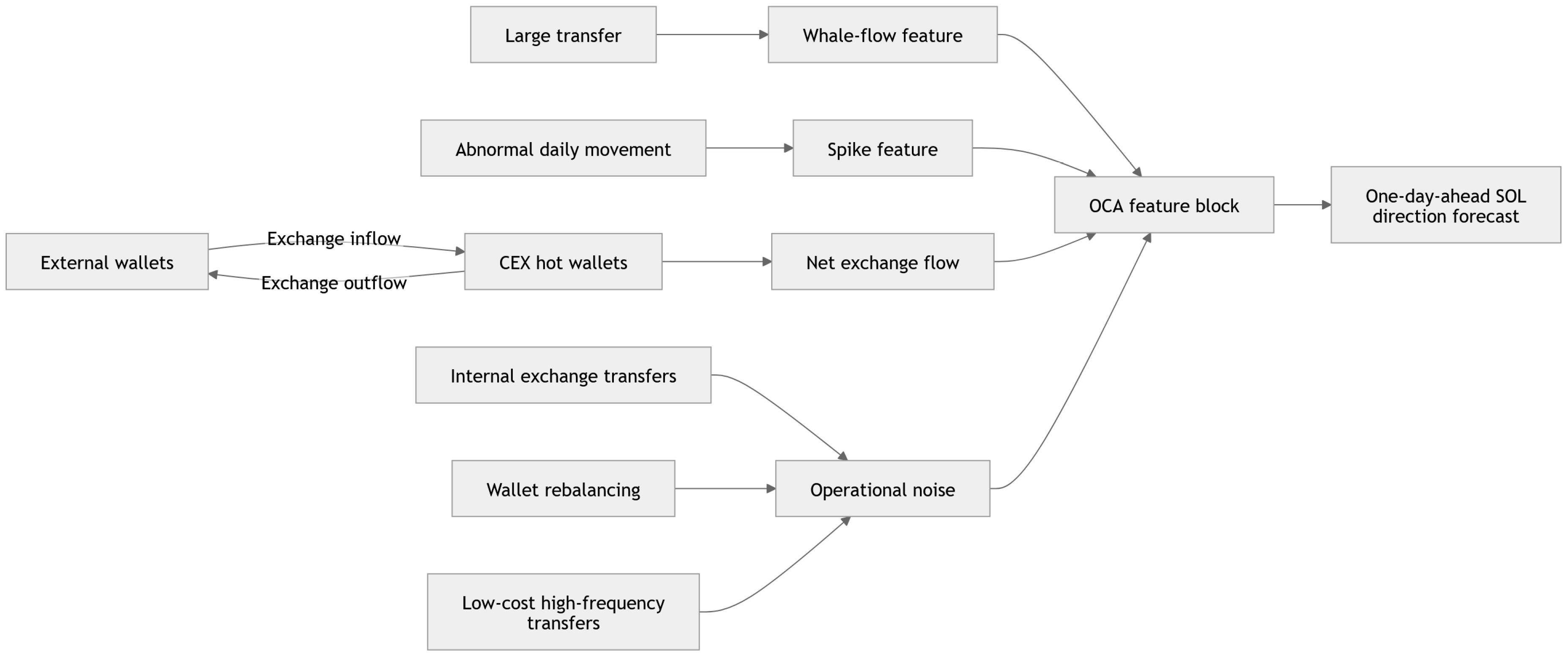
Figure 1 illustrates the exchange-flow mechanism employed in the forecasting framework. It links transfers between external wallets and centralized-exchange hot wallets to net-flow measures, large-transfer activity, abnormal movement indicators, and operational-noise channels. This structure explains why OCA variables are economically meaningful while still requiring rigorous out-of-sample validation: the same transaction infrastructure may simultaneously contain investor-flow information and exchange-internal operational activity.

Differences across cryptocurrency ecosystems further limit the transferability of existing results. Evidence on feature sensitivity [19], changing market conditions [22], cross-venue segmentation [27], and algorithmic liquidity [28,29] suggests that findings for Bitcoin or Ethereum may not generalize directly to Solana. The assets differ in transaction costs, throughput, ecosystem composition, market structure, and the maturity of address-labeling systems. Exchange-flow effects must therefore be estimated at the asset level rather than inferred from evidence for other cryptocurrencies.

Explainable artificial intelligence provides an additional means of evaluating whether selected predictors have an economically coherent role. XAI methods can help distinguish persistent and interpretable variables from unstable model artifacts in cryptocurrency applications [30,31] and broader financial forecasting [32]. This distinction is particularly important when exchange-wallet data combine investor behavior with operational traffic.

2.4. The Solana-Specific Forecasting Gap

Evidence on centralized-exchange flows as a distinct predictor block for short-horizon SOL returns remains limited. Existing studies focus primarily on Bitcoin, combine heterogeneous on-chain variables, or emphasize model architecture rather than the incremental value of exchange flows. Whether labeled Solana exchange-wallet activity contains information beyond conventional market and technical predictors is therefore unresolved.

This study evaluates Solana exchange flows both independently and alongside technical, market, macro-financial, investor-attention, Bitcoin-related, and VMD predictors. Its asset-specific design avoids cross-chain comparisons that could be confounded by differences in transaction mechanics, wallet-label coverage, and address completeness. Extending Bitcoin-centered evidence [1,5] and research on changing market conditions [22], the analysis compares unrestricted OCA with flow, volume, whale, network, and abnormal-spike subblocks under chronological validation.

3. Research Hypotheses

Section 5 defines the forecasting target and evaluation protocol. Let $B$, $T$, and $O$ denote the Baseline, TA, and OCA feature blocks, respectively. Mean feature-set performance and marginal OCA contributions are defined in Section 5.4.

H1 tests the standalone predictive value of OCA. Support requires OCA to exceed both the no-skill balanced-accuracy benchmark and the non-OCA Baseline:

$$H1:Q_{BA}(O)>0.5 \mathrm{and} Q_{BA}(O)>Q_{BA}(B);$$

(1)

$$\mathrm{strong} H1:Q_{BA}(O)\ge Q_{BA}(T).$$

H2 tests whether OCA adds information to predictors already available to the forecasting system. It is supported when adding $O$ improves balanced accuracy or ROC-AUC relative to $B$, $T$, or $B\cup T$:

$$H2:\exists S\in \{B,T,B\cup T\},q\in \{BA,ROC\text{-}AUC\}:{\Delta }_q(O|S)>0.$$

(2)

This hypothesis assesses whether exchange flows contain information not captured by market, macro-financial, attention, Bitcoin-related, VMD, or technical predictors.

H3 tests whether OCA improves transaction-cost-adjusted economic performance. Let $\mathsf{\Pi }(g)$ contain the mean holdout return, Sharpe ratio, signed maximum drawdown, and win rate defined in Section 5.4. Specification $A$ economically dominates $B$, denoted $A{\succ }_{E}B$, when it is no worse on all four measures and strictly better on at least one:

$$H3:\mathsf{\Pi }(S\cup O){\succ }_E\mathsf{\Pi }(S) \mathrm{for} \mathrm{some} S\in \{B,T,B\cup T\}, \mathrm{or} \mathsf{\Pi }(O){\succ }_E\mathsf{\Pi }(B).$$

(3)

H4 tests whether useful OCA information is concentrated in compact subblocks. Let

$$\begin{gathered} O_t=O_t^{flow}\cup O_t^{volume}\cup O_t^{whale}\cup O_t^{network}\cup O_t^{spike}, \\ K=\{flow,volume,whale,network,spike\}. \end{gathered}$$

The hypothesis is

$$H4:\underset{k\in K}{\mathrm{m}\mathrm{a}\mathrm{x}} Q_{BA}(O^k)>Q_{BA}(O),$$

(4)

and/or

$$Q_{BA}(O^{flow}\cup O^{volume}\cup O^{spike})>Q_{BA}(O).$$

(5)

H4 therefore tests whether informative OCA signals are concentrated in interpretable subblocks rather than diluted by operational noise.

4. Data

4.1. Market, Macro-Financial, Attention, and VMD Variables

The daily dataset combines market variables, macro-financial controls, investor attention, decomposition-based price features, and Solana exchange flows. Except for the ex post whale threshold defined in Section 4.2, predictors dated $t$ use only information available by the end of that date to forecast return direction on $t+1$.

The market block contains daily SOL price and trading-volume variables together with Bitcoin-related market variables. SOL variables provide the asset-specific price history from which returns, technical indicators, and decomposition-based features are derived. Bitcoin variables are included as a broad cryptocurrency-market factor, since Bitcoin often captures common variation in market-wide risk appetite, momentum, and liquidity. Their inclusion reduces the possibility that general cryptocurrency-market conditions are incorrectly attributed to Solana-specific exchange flows.

The macro-financial block consists of the U.S. Dollar Index, the S&P 500 index, and the Federal funds rate. These variables represent dollar strength, aggregate risky-asset conditions, and the monetary-policy environment. Since cryptocurrencies trade continuously, whereas traditional financial variables are updated only on trading or policy dates, the macro-financial series are mapped to the daily calendar by carrying forward the latest available observation. This procedure preserves the information constraint because only values known at the forecast origin are used.

Investor attention is measured by the Google Trends index for the term “Solana.” A Bitcoin halving-cycle index controls for broader cryptocurrency-market conditions.

The baseline block further includes rolling Variational Mode Decomposition (VMD) features extracted from the SOL closing-price series. Let $P_{\tau }$ denote the SOL closing price, and let $W_t=\{t-W+1,\dots ,t\}$ denote the rolling estimation window available at date $t$. The VMD representation used in the forecasting design is

$$\begin{gathered} P_{\tau }={\displaystyle \sum _{k=1}^K}{u}_{k,\tau }^{\left(t\right)}+{\epsilon }_{\tau }^{\left(t\right)},\tau \in W_t, \\ {V}_t=\left(u_{1,t}^{\left(t\right)},\dots ,u_{K,t}^{\left(t\right)}\right),K=10. \end{gathered}$$

Here, $u_{k,\tau }^{\left(t\right)}$ is the $k$-th mode estimated using only observations inside $W_t$, ${\epsilon }_{\tau }^{\left(t\right)}$ is the residual component, and $V_t$ contains the final observed value of each mode. Estimating the decomposition separately on each rolling window prevents the VMD features from using future prices.

The Baseline information set is

$$B_t=[M_t,C_t,A_t,H_t,V_t],$$

where $M_t$ contains SOL and Bitcoin market variables, $C_t$ contains macro-financial controls, $A_t$ denotes investor attention, $H_t$ is the halving-cycle index, and $V_t$ contains the rolling VMD modes.

The VMD implementation is fixed across all experiments. The number of modes is $K=10$, with $\alpha =2000$, $\tau =0$, initialization parameter $init=1$, tolerance ${10}^{-7}$, and a rolling window of $W=200$ daily observations. For each forecast date $t$, the decomposition is estimated only on the rolling history ending at $t$, and the final values of the ten modes are stored as $vmd\_1,\dots ,vmd\_10$. These settings define the VMD component of $B_t$ in every feature specification that includes the baseline block.

4.2. Solana Exchange-Flow Data and OCA Variables

The on-chain component consists of transaction-level SOL transfers involving labeled centralized-exchange hot wallets. Raw transaction histories cover the period from 1 August 2020 to 11 November 2025, while the main forecasting sample begins in January 2021. The earlier observations provide the initial history required to construct lagged and rolling on-chain analysis (OCA) variables without using future information.

The labeled exchange-wallet set contains 101 hot wallets associated with major centralized exchanges, including Coinbase, Kraken, OKX, Huobi, Gate, Crypto.com, Bitfinex, Gemini, Bybit, Bitstamp, Bitget, MEXC, Upbit, Bithumb, CoinEx, and Poloniex. The analysis focuses on hot wallets because they are used for operational deposits, withdrawals, and exchange-side liquidity management. Cold wallets are excluded to restrict the measurement framework to routine exchange-facing transaction activity.

Transfer histories for each labeled wallet are obtained through the Solscan API. The resulting dataset contains more than 41 million SOL transfers. Transactions of 1 SOL or less are excluded to reduce the influence of micro-transfers and economically negligible activity. The retained observations therefore comprise transfers above 1 SOL for which at least one endpoint belongs to the labeled exchange-wallet set.

Each transfer is classified according to its direction relative to the labeled wallet set. A transfer from an external address to a labeled exchange hot wallet is classified as an exchange inflow. Conversely, a transfer from a labeled exchange hot wallet to an external address is classified as an exchange outflow. Transfers between two labeled exchange wallets are not included in either measure because they may represent inter-exchange or internal operational movements rather than a change between exchange-side and external holdings. Transaction-level observations are aggregated by day to match the frequency of the market, macro-financial, investor-attention, and VMD predictors.

Let $D_t$ be the set of filtered SOL transfers observed on day $t$. For transfer $i\in D_t$, let $q_i$ denote the transfer amount, $sende{r}_i$ and $receive{r}_i$ denote the sending and receiving addresses, and $E_X$ denote the labeled set of centralized-exchange hot wallets. Daily exchange inflow and outflow are defined as

$$\begin{gathered} I{n}_t=\sum _{i\in D_t}{q}_i \mathbf{1}\{sende{r}_i\notin E_X,receive{r}_i\in E_X\}, \\ Ou{t}_t=\sum _{i\in D_t}{q}_i \mathbf{1}\{sende{r}_i\in E_X,receive{r}_i\notin E_X\}. \end{gathered}$$

The daily net flow is defined as

$$N{F}_t=I{n}_t-Ou{t}_t.$$

The OCA information set comprises flow, transfer-volume and transfer-size, whale-activity, network-activity, and spike variables. Appendix A,

Table A1. Complete OCA feature dictionary (47 predictors).

Family	Variables	Interpretation
Network activity	tx_count; address_count; receiver_count; unique_addresses; address_entropy; burstiness; velocity_tpm	Transaction intensity, breadth of participation, address concentration, and irregularity of transfer timing.
Flow	inflow; outflow; net_flow; inflow_rel; outflow_rel; inflow_ratio; outflow_ratio; rolling_netflow_3d; rolling_netflow_24d; rolling_netflow_3d_normed; rolling_netflow_24d_normed	Daily flow levels and three-day and 24-day rolling sums; _3d and _24d are retained implementation names.
Volume and size	total_volume; total_volume_rel; rolling_volume_3d; rolling_volume_24d; avg_tx_amount; mean_amount; std_amount; median_amount; max_amount; min_amount; value_volatility	Daily transfer-size statistics and three-day and 24-day rolling volume sums.
Whale	whale_tx_count; whale_volume; whale_volume_share; avg_whale_amount	Transfers above the within-quarter 95th percentile of transaction amount; interpreted ex post.
Spike	spike_tx; spike_volume; spike_netflow; spike_inflow; spike_outflow; spike_unique_addresses; spike_whales; rolling_tx_mean_spike; rolling_vol_mean_spike; rolling_netflow_mean_spike; rolling_inflow_mean_spike; rolling_outflow_mean_spike; rolling_addresses_mean_spike; rolling_whale_share_mean_spike	Seven-day rolling means and ratios of current activity to those means.

provides the complete feature dictionary. Variables with the implementation suffixes _3d and _24d denote three-day and 24-day rolling sums, respectively, while spike ratios use seven-day rolling means. All rolling windows end on the forecast date.

Whale transfers exceed the 95th percentile of transaction amount within the corresponding calendar quarter. Because this threshold is calculated from the completed quarter, whale variables are ex post descriptive features rather than strictly real-time predictors.

For a daily variable $z_t$, let ${\overline{z}}_{t,7}$ denote its mean over the current and preceding six observations, with shorter windows at the sample origin. The spike ratio is

$$Spik{e}_t(z)={\displaystyle \frac{z_t}{{\overline{z}}_{t,7}}}.$$

Zero denominators are treated as missing before the common forward-fill and zero-imputation procedure.

The OCA block approximates observable centralized-exchange SOL flows. The wallet set may omit unidentified, newly created, or inactive exchange addresses, and retained transfers may include internal exchange activity. These limitations require cautious interpretation of OCA results.

5. Empirical Design

5.1. Forecasting Target and Information Timing

The empirical design tests whether Solana exchange-flow predictors improve one-day-ahead forecasts of SOL return direction under chronological evaluation. All predictors and targets are defined at the daily frequency. Let $P_t$ denote the SOL closing price on date $t$. The next-day log return and direction target are

$$r_{t+1}=\mathrm{l}\mathrm{n}(P_{t+1}/P_t), y_{t+1}=\mathbf{1}\{r_{t+1}>0\}, X_t^g\in {\mathcal{F}}_t.$$

Here, $X_t^g$ is the predictor vector for feature specification $g$, and ${\mathcal{F}}_t$ is the information set available by the end of date $t$. It includes price and volume indicators, forward-filled macro-financial controls, Google Trends, rolling VMD components, and daily exchange-flow aggregates.

The completed-quarter whale threshold described in Section 4.2 is the only exception to strict real-time feature construction. Results from OCA-containing specifications that select whale variables are therefore interpreted as descriptive rather than strictly real-time.

For model family $m$, feature specification $g$, and holdout $h$, the probability and direction forecasts are

$${\widehat{p}}_{t+1}^{m,g,h}=f_{m,g,h}(X_t^g), {\widehat{y}}_{t+1}^{m,g,h}=\mathbf{1}\{{\widehat{p}}_{t+1}^{m,g,h}\ge 0.5\}.$$

The model $f_{m,g,h}$ is estimated exclusively from observations preceding holdout $h$. All feature specifications are evaluated over identical holdout dates, ensuring that their performance is compared under the same market conditions.

Binary forecasts are mapped directly into long and short positions:

$${\pi }_t^{\left(m,g,h\right)}=2{\widehat{y}}_{t+1}^{\left(m,g,h\right)}-1\in \{-1,+1\}.$$

This mapping permits joint evaluation of classification accuracy and transaction-cost-adjusted trading performance.

5.2. Feature Specifications

The empirical experiment compares seven feature specifications. Let $B_t$ denote the baseline block, $T_t$ the technical-analysis block, and $O_t$ the Solana exchange-flow OCA block. The evaluated specification set is

$$G=\{B,T,O,B\cup O,B\cup T,O\cup T,B\cup T\cup O\}.$$

Baseline contains 17 market, macro-financial, investor-attention, Bitcoin-related, and VMD predictors. TA contains 56 indicators derived from SOL prices and trading volume, while OCA contains 47 exchange-flow and activity variables. The Full specification combines all three blocks and contains 120 candidate predictors before training-only feature selection:

$$\left|B\right|=17, \left|T\right|=56, \left|O\right|=47, |B\cup T\cup O|=120.$$

These comparisons correspond directly to the hypotheses. H1 evaluates the standalone predictive value of OCA. H2 tests its incremental contribution through Baseline + OCA versus Baseline, OCA + TA versus TA, and Full-versus-Baseline + TA. H3 evaluates transaction-cost-adjusted performance, and H4 examines whether OCA information is concentrated in interpretable subblocks.

The OCA block is divided into five interpretable subblocks: flow variables measuring inflows, outflows, and net flows; volume and transfer-size variables; whale-activity variables capturing large and concentrated transfers; network-activity variables; and spike variables measuring abnormal movements relative to recent history. Formally,

$$O_t=O_t^{flow}\cup O_t^{volume}\cup O_t^{whale}\cup O_t^{network}\cup O_t^{spike}.$$

5.3. Models and Training Protocol

The empirical analysis includes three tree-based classifiers—CatBoost, XGBoost, and Random Forest—and two recurrent neural-network architectures, LSTM and BiLSTM. Elastic Net Logistic Regression is included as a regularized linear benchmark. This model set permits comparison between nonlinear tabular methods, sequential architectures, and a sparse linear specification under a common chronological evaluation protocol.

The tabular models use fixed configurations across all feature specifications and holdouts. CatBoost is estimated with 260 iterations, a maximum tree depth of 5, a learning rate of 0.045, and an L2 leaf-regularization coefficient of 6. XGBoost uses 220 trees, a maximum depth of 3, a learning rate of 0.035, row subsampling of 0.85, column subsampling of 0.75, L1 regularization of 1, and L2 regularization of 4. Random Forest contains 500 trees with a maximum depth of 8, a minimum leaf size of 5, square-root feature sampling, and balanced-subsample class weights. Elastic Net Logistic Regression uses the SAGA solver with an L1 ratio of 0.5, $C=0.2$, balanced class weights, and a maximum of 5000 iterations.

The LSTM and BiLSTM models use 30-day historical input sequences. Each architecture consists of one recurrent layer followed by dropout, a fully connected layer with 32 ReLU units, a second dropout layer, and a single-unit binary output layer. The models are trained using Adam with weight decay of ${10}^{-5}$, a batch size of 64, and a maximum of 30 epochs. Early stopping is applied with a patience of five epochs, and gradients are clipped at 1.0.

Neural-network hyperparameters are selected using only the pre-holdout training sample. The search considers recurrent hidden dimensions of $\left\{32,64,96\right\}$, dropout rates of $\left\{0,0.2\right\}$, and learning rates of $\left\{0.001,0.0005\right\}$. Up to 12 configurations are evaluated using an 85:15 chronological training-validation split. The selected configuration is then fixed before the corresponding holdout is evaluated. All stochastic components use random seed 42.

For each holdout, preprocessing, feature selection, scaling, hyperparameter selection, and model estimation use only preceding observations. Fitted transformations and parameters are then applied unchanged to the holdout. The recurrent models use sequences ending at forecast origin $t$. BiLSTM processes both directions within this observed 30-day sequence but receives no information from $t+1$ or later dates.

Feature selection is repeated for each feature specification and holdout. Constant predictors are removed, after which predictors with absolute Spearman correlation above 0.85 are clustered. Each cluster is represented by the variable with the highest univariate mutual information with the training target.

The remaining predictors are ranked across four training-only TimeSeriesSplit folds separated by a seven-day gap. Within each fold, a 130-iteration CatBoost model produces mean absolute SHAP importance and five-repeat permutation importance evaluated by validation F1. Both importance vectors are min–max normalized within the fold. Temporal stability is the proportion of folds in which normalized SHAP or permutation importance reaches 0.5, and mutual information is normalized over the training sample. Aggregate importance is the unweighted mean of normalized SHAP importance, permutation importance, temporal stability, and mutual information.

Predictors with aggregate importance of at least 0.55 are retained, subject to a minimum of 15 variables. Candidate sets containing 15, 20, 30, or 45 top-ranked predictors, together with the threshold-selected set, are evaluated through inner time-series validation using a 120-iteration CatBoost model. The smallest set attaining the highest mean F1 is selected.

Within each feature specification and holdout, the selected predictor set is passed unchanged to all model families. This procedure ensures that comparisons across CatBoost, XGBoost, Random Forest, LSTM, BiLSTM, and Elastic Net reflect differences in model structure rather than differences in the information supplied to each model. Elastic Net follows the same training-only preprocessing and validation timing as the nonlinear and sequential models.

5.4. Out-of-Sample Evaluation and Descriptive Market States

Out-of-sample performance is evaluated over four non-overlapping, half-open intervals: [1 November 2023, 1 May 2024), [1 May 2024, 1 November 2024), [1 November 2024, 1 May 2025), and [1 May 2025, 1 November 2025). Each boundary date belongs only to the later holdout. The periods are descriptively characterized as an upward trend, consolidation, growth followed by reversal, and volatile recovery.

The evaluation uses a blocked expanding-origin design. For each holdout, models are fitted using only preceding observations and remain fixed throughout the evaluation block. The training sample expands before the next holdout.

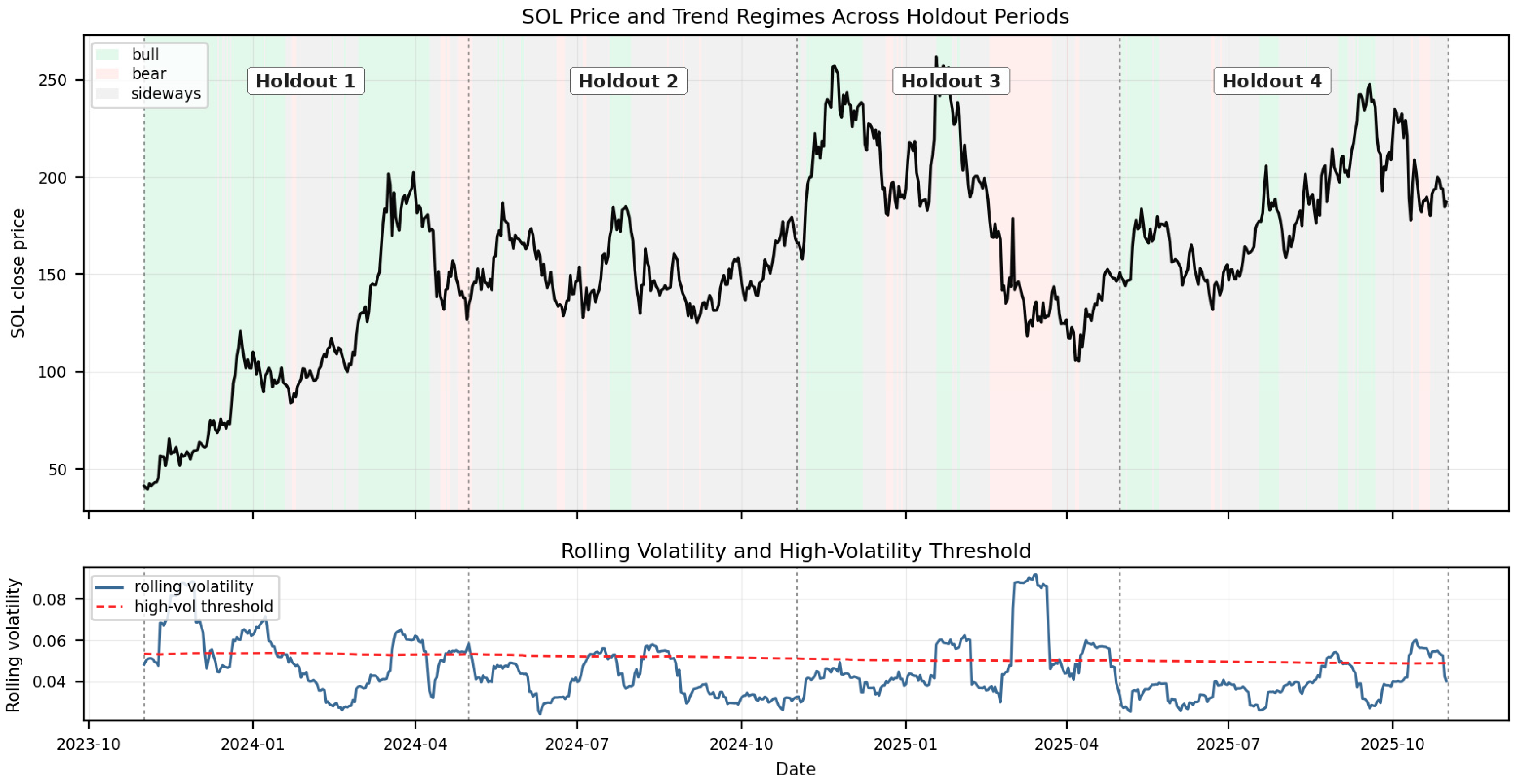
Figure 2 presents the SOL price path, daily trend classifications, and volatility conditions across the four holdouts.

Table 1. Holdout-period economic interpretation.

Holdout	Period	Descriptive Market State	Economic Interpretation
Holdout 1	[1 November 2023, 1 May 2024)	Upward trend	A sustained positive trend during which long-biased or price-derived signals may perform particularly well.
Holdout 2	[1 May 2024, 1 November 2024)	Consolidation	A comparatively range-bound period in which directional predictability may be weaker.
Holdout 3	[1 November 2024, 1 May 2025)	Growth and reversal	A period of rapid appreciation followed by reversal, providing context for evaluating exchange-flow signals during repricing.
Holdout 4	[1 May 2025, 1 November 2025)	Volatile recovery	A recovery characterized by elevated volatility and intermittent pullbacks.

summarizes their broader market interpretation.

The trend classification in Figure 2 is based on the 30-day simple return,

$$m_t={\displaystyle \frac{P_t}{P_{t-30}}}-1.$$

The time-varying trend threshold is

$$q_t=0.35{\widehat{\sigma }}_{t-1}^{\mathrm{e}\mathrm{x}\mathrm{p}}(m),$$

where ${\widehat{\sigma }}_{t-1}^{\mathrm{e}\mathrm{x}\mathrm{p}}(m)$ is the expanding standard deviation of $m$, based on at least 90 observations and lagged by one day. Date $t$ is classified as bull when $m_t>q_t$, bear when $m_t<-q_t$, and sideways otherwise.

Rolling volatility is the 20-day standard deviation of one-day simple SOL returns. A date is classified as high-volatility when rolling volatility exceeds its expanding median, calculated from at least 90 observations and lagged by one day.

These classifications provide descriptive context. Forecast evaluation is not conditioned on market state, and the analysis does not test whether OCA importance varies systematically across states.

Classification performance is reported using balanced accuracy, F1 score, Matthews correlation coefficient, and ROC-AUC. Balanced accuracy is emphasized because the up and down classes may be uneven within a holdout:

$$BA=0.5\left[{\displaystyle \frac{TP}{TP+FN}}+{\displaystyle \frac{TN}{TN+FP}}\right].$$

MCC penalizes one-sided prediction rules, while ROC-AUC evaluates the probability ranking implied by each model.

For metric $q$, $Q_q(g)$ denotes the mean score of feature specification $g$ across model families and holdouts. The marginal contribution of OCA to reference specification $S$ is

$${\Delta }_q(O|S)=Q_q(S\cup O)-Q_q(S).$$

Economic performance is calculated from forecast-implied positions and simple daily SOL returns:

$$R_{t+1}={\displaystyle \frac{P_{t+1}}{P_t}}-1,{\pi }_t=2{\widehat{y}}_{t+1}-1.$$

With proportional transaction cost $c$, the net strategy return is

$$R_{t+1}^{\mathrm{n}\mathrm{e}\mathrm{t}}={\pi }_t{R}_{t+1}-c|{\pi }_t-{\pi }_{t-1}|.$$

Unless otherwise stated, the trading-performance analyses use $c=0.001$, equivalent to 0.10% per unit change in position. An unchanged position incurs no cost, whereas a reversal incurs $2c$.

Terminal holdout return is the arithmetic sum of daily net returns from the unconstrained long–short simulation. It is not compounded wealth. A return below $-100\%$ therefore indicates a severe cumulative simulated loss rather than a feasible self-financing portfolio outcome.

For the main-model trading summary, each holdout statistic is first averaged across the five main model families. Let ${\overline{R}}_h(g)$ denote the resulting return for feature specification $g$ in holdout $h$. Panel B reports the corresponding Elastic Net results without cross-model averaging. The sum, mean, and best holdout returns are calculated from the four ${\overline{R}}_h(g)$ values. The cross-holdout product statistic is

$$A(g)={\displaystyle \prod _{h=1}^4}\left[1+{\overline{R}}_h(g)\right]-1.$$

Because the underlying holdout returns are arithmetic sums from an unconstrained simulation, $A(g)$ is descriptive and should not be interpreted as compounded portfolio wealth.

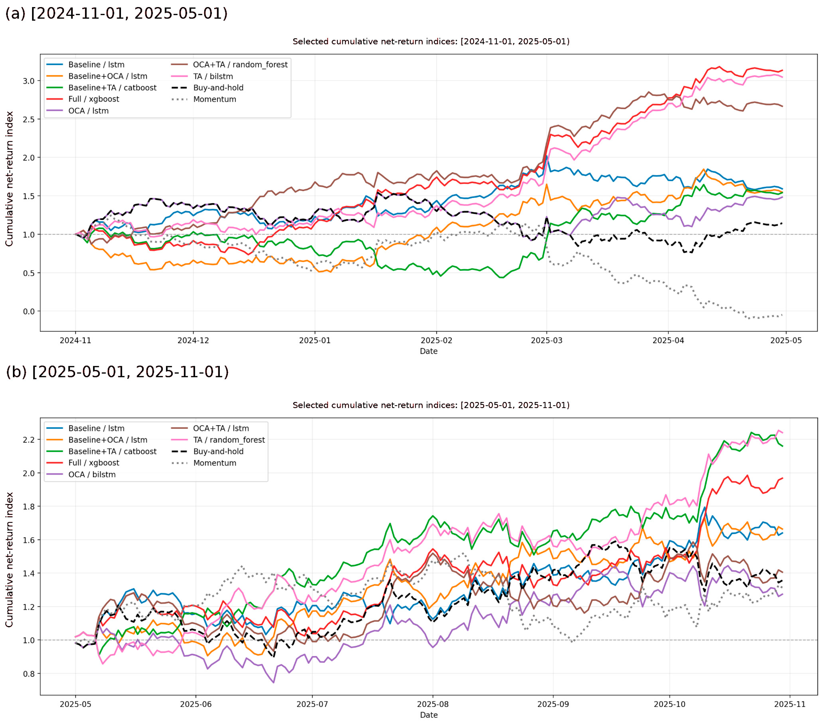
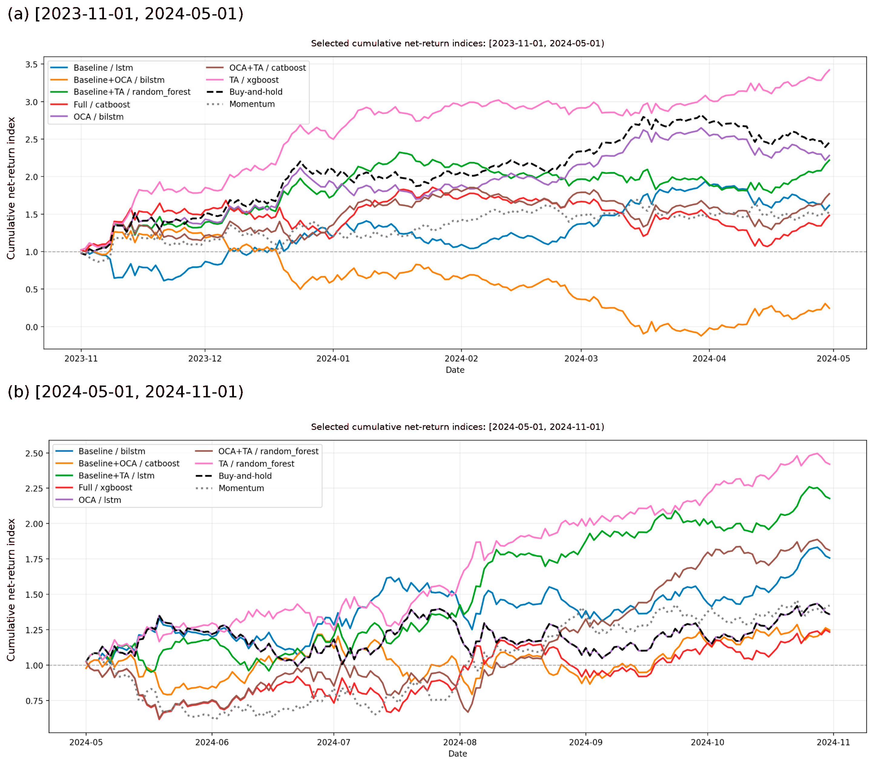
Figure 3 and Figure 4 plot the cumulative net-return index

$$C_t=1+\sum _{\tau \le t}{R}_{\tau }^{\mathrm{n}\mathrm{e}\mathrm{t}}$$

at $c=0.001$. These paths follow the same arithmetic-return convention and are not self-financing equity curves.

Turnover is the mean absolute daily change in position. The annualized Sharpe ratio equals $\sqrt{365}$ times the mean daily net return divided by its standard deviation. The simulation includes proportional transaction costs but excludes bid–ask spreads, slippage, market impact, funding rates, borrow availability, and short-borrowing costs. The reported trading results are therefore interpreted as friction-adjusted model comparisons rather than implementable portfolio returns.

The paired-comparison analysis summarizes 20 matched model–holdout differences from five model families and four holdouts. Each augmented-minus-reference difference is calculated within the same model family and holdout. The reported 95% intervals are the 2.5th and 97.5th percentiles of 1000 bootstrap resamples of these matched differences. Two-sided p-values equal twice the smaller empirical bootstrap tail probability relative to zero. Because the comparisons share holdouts and overlapping training histories, the paired-comparison analysis provides provides descriptive robustness evidence rather than population-level inference. Elastic Net is excluded.

6. Results

6.1. Average Predictive Performance

Panel A of

Table 2. Average out-of-sample classification performance by feature set and benchmark type. Panel (A). Main nonlinear and sequential model families; Panel (B). Elastic Net Logistic Regression benchmark.

(A)
Feature Set	Best Observed Balanced Accuracy	Precision (up)	Recall (up)	F1	Balanced Accuracy	MCC	ROC-AUC
TA	0.601	0.550	0.578	0.535	0.545	0.093	0.572
Baseline + TA	0.556	0.527	0.554	0.489	0.513	0.026	0.542
OCA + TA	0.580	0.529	0.537	0.474	0.513	0.025	0.520
Full	0.541	0.521	0.513	0.435	0.505	0.011	0.510
Baseline	0.535	0.492	0.556	0.468	0.491	−0.019	0.483
Baseline + OCA	0.514	0.489	0.530	0.459	0.487	−0.026	0.480
OCA	0.495	0.496	0.524	0.451	0.474	−0.057	0.475
(B)
Feature Set	F1	Balanced Accuracy	Precision (up)	Recall (up)	MCC	ROC-AUC	Mean Number of Features
OCA + TA	0.507	0.555	0.595	0.464	0.118	0.589	37.50
TA	0.532	0.555	0.584	0.503	0.114	0.595	21.00
Full	0.485	0.550	0.593	0.422	0.107	0.584	30.00
Baseline + TA	0.421	0.539	0.578	0.332	0.083	0.582	22.50
Baseline	0.421	0.523	0.545	0.383	0.049	0.532	15.25
Baseline + OCA	0.289	0.501	0.499	0.215	−0.005	0.497	23.75
OCA	0.277	0.475	0.465	0.245	−0.058	0.473	17.50

reports mean out-of-sample classification performance across the five nonlinear and sequential model families. TA leads all feature specifications in balanced accuracy (0.545), MCC (0.093), and ROC-AUC (0.572) and achieves the highest balanced accuracy observed for any model–holdout combination (0.601). Baseline + TA is the strongest combined specification without OCA but trails TA on each metric.

OCA-based specifications perform less well. OCA + TA and Baseline + TA have the same mean balanced accuracy (0.513), but OCA + TA records lower MCC and ROC-AUC. Full achieves a balanced accuracy of 0.505, only marginally above the no-skill benchmark. Baseline + OCA underperforms Baseline, while standalone OCA has balanced accuracy and ROC-AUC below 0.50 and negative MCC. The unrestricted OCA block therefore provides no reliable standalone predictive advantage.

Table 2 also reports positive-class precision, recall, and F1. The overall share of positive-return observations is 0.516. Across the four half-open holdouts, the corresponding shares are 0.533, 0.516, 0.492, and 0.525. Thus, no holdout is dominated by either return-direction class.

Panel B of Table 2 shows a similar feature-block pattern for Elastic Net. TA and OCA + TA share the highest balanced accuracy (0.555). TA achieves higher F1 and ROC-AUC, whereas OCA + TA records a slightly higher MCC. Full and Baseline + TA outperform the standalone Baseline and OCA specifications. Standalone OCA remains below the balanced-accuracy no-skill benchmark and has negative MCC. Elastic Net therefore supports the broad pattern in Panel A, although the metric-specific rankings differ.

Overall, Table 2 shows that standalone OCA performs poorly and trails both Baseline and TA on average. H1 is therefore unsupported. The stronger version of H1 is also unsupported because OCA achieves lower mean balanced accuracy than TA (0.474 versus 0.545).

6.2. Incremental Contribution of Feature Blocks

Table 3. Paired incremental comparisons between feature specifications.

Comparison	Delta Balanced Accuracy	95% CI	p-Value	Positive/N	Delta ROC-AUC	95% CI	p-Value	Positive/N
Baseline + TA—Baseline	+0.0225	[−0.0556; 0.1001]	0.4060	13/20	+0.0588	[−0.0360; 0.1534]	0.2899	16/20
Baseline + OCA—Baseline	−0.0038	[−0.0727; 0.0659]	0.5514	8/20	−0.0033	[−0.0946; 0.0860]	0.6368	8/20
OCA + TA—TA	−0.0324	[−0.1044; 0.0369]	0.3350	5/20	−0.0519	[−0.1305; 0.0186]	0.2522	3/20
Full—Baseline + TA	−0.0084	[−0.0759; 0.0618]	0.4968	9/20	−0.0321	[−0.1161; 0.0488]	0.3924	4/20

evaluates H2 using paired comparisons constructed within the same model family and holdout. Adding TA to Baseline produces positive mean differences in balanced accuracy ($+0.0225$) and ROC-AUC ($+0.0588$). The differences are positive in 13 of 20 and 16 of 20 matched comparisons, respectively. However, both 95% intervals include zero, and the corresponding bootstrap $p$-values do not indicate a consistent improvement.

Adding OCA to Baseline produces mean differences of −0.0038 in balanced accuracy and −0.0033 in ROC-AUC, with positive differences in 8 of 20 comparisons for both metrics. OCA + TA also underperforms TA on average: balanced accuracy decreases by 0.0324 and ROC-AUC by 0.0519, with positive differences in only 5 of 20 and 3 of 20 comparisons, respectively. Full trails Baseline + TA by 0.0084 in balanced accuracy and 0.0321 in ROC-AUC. None of the OCA-related intervals excludes zero.

Taken together, the paired results in Table 3 provide no evidence that OCA delivers a stable average incremental improvement over either Baseline or TA. H2 is therefore not supported as an average out-of-sample effect. Any narrower contribution associated with particular OCA subblocks or holdout periods requires separate matched comparisons and should not be inferred from these aggregate results.

6.3. Trading Performance

Panel A of

Table 4. Trading performance by feature set and benchmark type. Panel (A). Main nonlinear and sequential model families. Panel (B). Elastic Net Logistic Regression benchmark.

(A)
Feature Set/Strategy		Sum Holdout Returns	Cross-Holdout Product	Best Holdout Return	Mean Holdout Return	Mean Sharpe	Mean Max DD	Mean Win Rate
TA		4.805	22.468	5.828	1.201	2.691	−0.295	0.543
Baseline + TA		2.033	4.171	2.617	0.508	1.195	−0.399	0.512
OCA + TA		1.414	2.351	2.775	0.353	0.815	−0.464	0.507
Full		0.983	1.410	3.163	0.246	0.588	−0.500	0.498
Baseline		−1.107	−0.727	0.229	−0.277	−0.621	−0.601	0.483
Baseline + OCA		−1.845	−0.916	−0.182	−0.461	−1.038	−0.637	0.475
OCA		−2.105	−0.950	−0.288	−0.526	−1.208	−0.643	0.468
(B)
Feature Set	Sum Holdout Returns	Cross-Holdout Product	Best Holdout Return	Mean Holdout Return	Mean Sharpe	Mean Max DD	Mean Win Rate	Turnover
TA	6.187	33.141	2.788	1.547	3.423	−0.163	0.551	0.414
OCA + TA	5.070	22.804	2.123	1.268	2.826	−0.213	0.551	0.376
Full	4.663	18.571	2.011	1.166	2.612	−0.231	0.547	0.414
Baseline + TA	3.381	7.521	1.600	0.845	1.828	−0.344	0.529	0.365
Baseline	−0.024	−0.459	0.532	−0.006	0.100	−0.640	0.508	0.567
Baseline + OCA	−0.752	−0.734	0.370	−0.188	−0.502	−0.784	0.487	0.589
OCA	−2.710	−1.035	−0.068	−0.678	−1.404	−0.935	0.459	0.367

reports transaction-cost-adjusted performance across the five nonlinear and sequential model families. TA achieves the highest mean holdout return (1.201), the highest mean Sharpe ratio (2.691), and the least severe mean maximum drawdown (−0.295). Its descriptive cross-holdout product statistic is 22.468. Baseline + TA ranks second, with a mean holdout return of 0.508 and a mean Sharpe ratio of 1.195.

OCA + TA and Full produce positive mean returns and Sharpe ratios but underperform TA and Baseline + TA, respectively. Standalone OCA performs worst, with a mean holdout return of −0.526, a mean Sharpe ratio of −1.208, and a mean maximum drawdown of −0.643. Baseline + OCA also underperforms Baseline. OCA therefore fails to satisfy the economic-dominance criterion specified in H3.

Panel B of Table 4 shows a similar pattern for Elastic Net. TA achieves the highest mean holdout return (1.547), mean Sharpe ratio (3.423), and least severe mean maximum drawdown (−0.163). Its descriptive cross-holdout product statistic is 33.141. OCA + TA trails TA, whereas Full outperforms Baseline + TA within the Elastic Net benchmark. Standalone OCA again records the weakest performance.

The Full-versus-Baseline + TA result for Elastic Net is not reproduced consistently across the five main model families. Table 4 therefore does not establish H3 as a stable average out-of-sample effect: OCA-containing specifications provide no consistent economic advantage over their matched non-OCA benchmarks after transaction costs.

Table 5. Passive and naive trading benchmarks.

Benchmark	Terminal Out-of-Sample Return	Sharpe	Max Drawdown	Win Rate	Turnover
Always-up/buy-and-hold proxy	0.578	1.239	−0.296	0.516	0.000
Momentum	0.047	0.183	−0.537	0.511	0.938

places the model-based strategies in the context of passive and naive trading rules. The always-up strategy serves as a buy-and-hold proxy, while the momentum strategy uses the previous day’s return direction as the signal for the next day. Turnover measures the mean absolute change in position and therefore indicates each strategy’s exposure to transaction costs.

As shown in Table 5, the always-up benchmark achieves a terminal out-of-sample return of 0.578 and a Sharpe ratio of 1.239 without signal-driven turnover. The momentum rule produces a substantially lower return and Sharpe ratio while exhibiting considerably higher turnover. These benchmarks provide economic reference points for the model-based results in Table 4.

Table 6. Best strategy by Sharpe ratio within each out-of-sample period.

Period	Best Specification	Model	Sharpe	Terminal Holdout Return	Max Drawdown
[1 November 2023, 1 May 2024)	TA	XGBoost	4.748	2.421	−0.077
[1 May 2024, 1 November 2024)	TA	Random Forest	3.748	1.420	−0.140
[1 November 2024, 1 May 2025)	Full	XGBoost	4.486	2.132	−0.340
[1 May 2025, 1 November 2025)	TA	Random Forest	3.360	1.240	−0.182

reports the highest-Sharpe strategy in each holdout. TA-based strategies lead in three of the four periods. In the third holdout, Full XGBoost ranks first, with a Sharpe ratio of 4.486, a terminal holdout return of 2.132, and a maximum drawdown of −0.340.

Because Table 6 reports only the winning strategy in each holdout, it does not identify the incremental contribution of OCA.

Appendix B ranks the strongest individual model–feature combinations. TA-based Random Forest, CatBoost, XGBoost, and BiLSTM account for most of the leading aggregate results. Figure 3 and Figure 4 present selected cumulative net-return indices at $c=0.001$. Within each feature specification and holdout, the displayed model has the highest Sharpe ratio.

6.4. OCA Subblocks and Concentration of Signal

Table 7. OCA subblock performance.

Specification	Mean Balanced Accuracy	Mean ROC-AUC	Mean Sharpe	Mean Holdout Return	Interpretation
Flow Only	0.497	0.481	−0.534	−0.251	Best individual OCA subblock by balanced accuracy
Volume Only	0.489	0.482	−0.078	−0.018	Best OCA subblock by trading metrics
Spike Only	0.482	0.472	−0.668	−0.321	Weak standalone performance
Whale Only	0.482	0.470	−1.026	−0.484	Weak standalone group
Network Only	0.478	0.472	−0.932	−0.443	Weak standalone group
Flow + Volume + Spike	0.505	0.489	−0.216	−0.101	Best combined OCA subblock by classification
Flow + Whale + Spike	0.493	0.481	−0.514	−0.247	Moderate but unstable
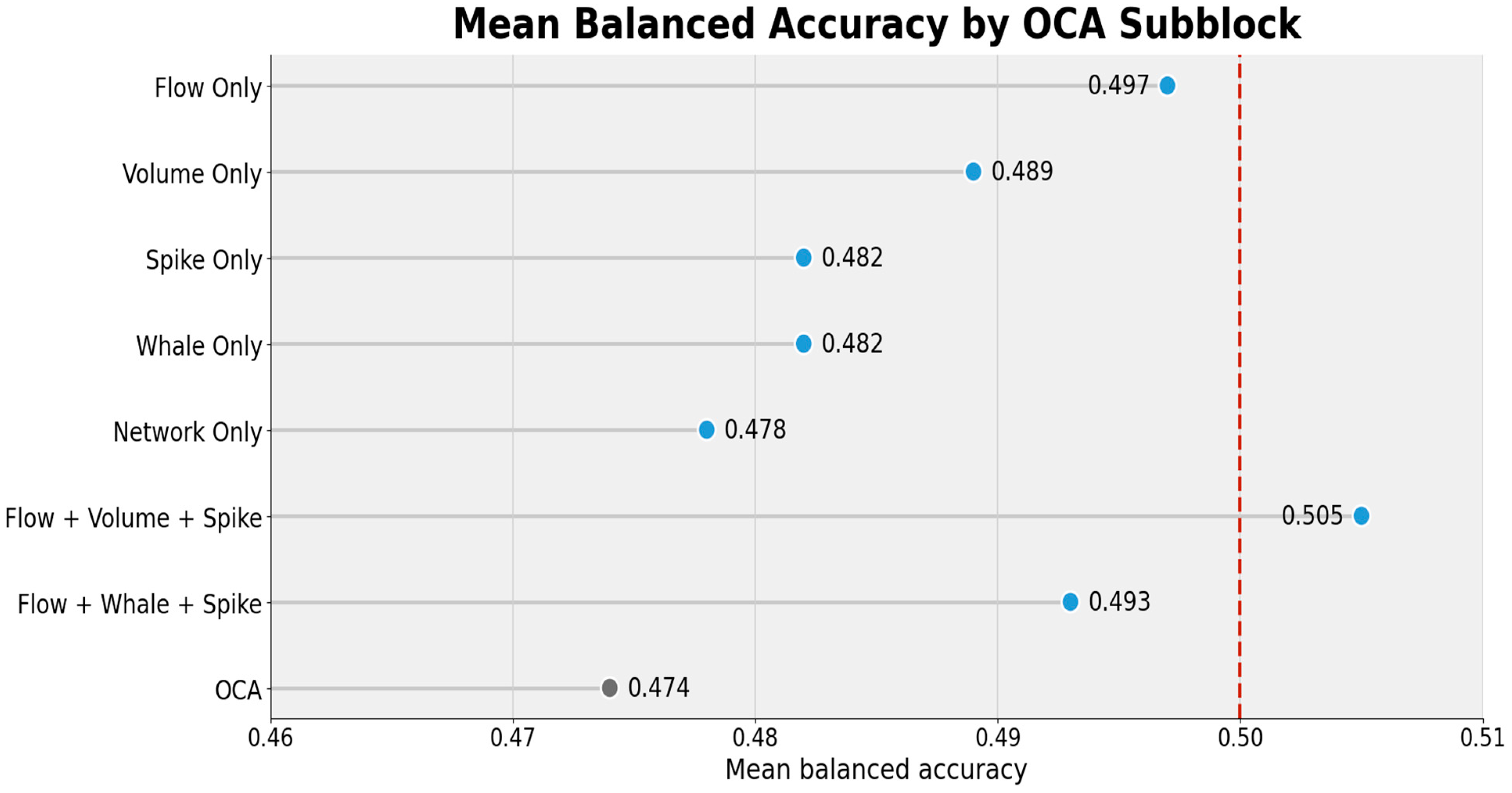
OCA	0.474	0.475	−1.208	−0.526	Weakest aggregate OCA performance

assesses whether predictive information is concentrated in compact OCA subblocks. Flow Only attains a mean balanced accuracy of 0.497, compared with 0.474 for OCA. Volume Only records the least negative mean Sharpe ratio (−0.078) and mean holdout return (−0.018). Flow + Volume + Spike achieves the highest mean balanced accuracy (0.505) and ROC-AUC (0.489) among the OCA subblocks, although its mean Sharpe ratio and mean holdout return remain negative. These results indicate limited descriptive gains without establishing robust subblock superiority.

Figure 5 compares the balanced-accuracy estimates in Table 7 with the 0.50 no-skill benchmark. Flow + Volume + Spike is the only specification to exceed this threshold, and only marginally, while its ROC-AUC and trading performance remain weak.

Table 8. Feature-level interpretability of selected OCA predictors.

Feature Set	Predictor	Group	Selection Rate	Mean SHAP	Mean Perm.	Mean Aggregate	Interpretation
OCA	rolling_netflow_mean_spike	Flow/net-flow	1.000	0.537	0.655	0.662	Net-flow-to-seven-day-mean ratio
OCA	rolling_outflow_mean_spike	Flow/net-flow	0.750	0.415	0.620	0.637	Outflow-to-seven-day-mean ratio
OCA	avg_whale_amount	Whale/size	1.000	0.229	0.609	0.581	Average size of large transfers
OCA	tx_count	Activity/volume	0.750	0.190	0.498	0.572	Transaction intensity
OCA	rolling_netflow_3d	Flow/net-flow	0.750	0.614	0.611	0.515	Three-day rolling net-flow sum (legacy name)
Full	MFI	Technical indicator	1.000	0.949	0.921	0.880	Dominant technical predictor under Full
Full	rolling_netflow_mean_spike	OCA: flow/net-flow	0.500	0.148	0.534	0.508	Net-flow-to-seven-day-mean ratio retained with TA
Full	rolling_volume_3d	OCA: volume/size	0.500	0.130	0.487	0.372	Three-day rolling transfer-volume sum (legacy name)
Full	burstiness	OCA: spike/activity	1.000	0.100	0.441	0.360	Irregular timing of exchange-flow activity
Full	std_amount	OCA: volume/size	1.000	0.025	0.351	0.316	Dispersion of transfer sizes

reports the highest-ranked OCA predictors retained within the OCA and Full specifications, together with the Money Flow Index (MFI), the leading technical predictor in the Full specification. The selection rate denotes the proportion of holdouts in which a predictor is retained. The SHAP, permutation, and aggregate scores are mean normalized training-only rankings across those holdouts. They do not represent holdout effects or tests of statistical significance. Because all model families use the same selected feature set, the rankings characterize each feature specification rather than individual model strategies.

Under Full, MFI has the highest mean aggregate importance. The net-flow-to-seven-day-mean ratio, three-day rolling transfer-volume sum, burstiness, and transfer-size dispersion are also retained alongside Baseline and TA predictors. Their retention identifies the OCA variables favored by the training-only ranking procedure but does not establish an incremental forecasting contribution. Evidence on incremental OCA value therefore rests on the matched feature-set comparisons in Table 3. The pairwise-test summaries reported later provide complementary evidence on the stability of pairwise performance differences across the evaluated models and forecasting rules.

Table 7 and Figure 5 satisfy the descriptive inequalities specified in H4, as selected OCA subblocks outperform OCA on particular metrics. Table 8 identifies the OCA variables retained under OCA and Full without establishing their individual predictive value. Given the weak classification results and negative transaction-cost-adjusted performance, H4 receives descriptive support only and does not imply robust predictive or economic value.

6.5. Robustness to Transaction Costs and Statistical Tests

Table 9. Mean holdout return under alternative transaction costs for selected TA-based strategies.

Strategy	c = 0.00%	c = 0.05%	c = 0.10%	c = 0.20%	c = 0.50%
TA + Random Forest	1.528	1.488	1.448	1.369	1.130
TA + CatBoost	1.540	1.498	1.457	1.374	1.125
TA + XGBoost	1.366	1.326	1.286	1.207	0.968
TA + BiLSTM	1.144	1.113	1.081	1.017	0.827

reports the arithmetic mean of the four holdout terminal returns for selected TA-based strategies under alternative proportional transaction costs. The $c=0.10\%$ column corresponds to the baseline cost assumption of $c=0.001$ per unit change in position and therefore matches the mean holdout returns reported in

Table A2. Best model–feature combinations by economic metrics.

Specification	Model	Mean Holdout Return	Sharpe	Max Drawdown
TA	Random Forest	1.448	3.334	−0.193
TA	CatBoost	1.457	3.287	−0.217
TA	XGBoost	1.286	2.900	−0.229
TA	BiLSTM	1.081	2.298	−0.339
Full	XGBoost	0.791	1.843	−0.295

. All four strategies retain positive mean holdout returns across the evaluated cost levels, although these returns decline monotonically as transaction costs increase.

Table 10. Summary of continuity-corrected McNemar and DM-style loss-differential tests.

Test	Comparison Object	Metric/Loss	Number of Tests	Significant at p < 0.05	Share Significant
McNemar	Binary forecasts	Disagreement of classification errors	588	25	0.043
DM-style loss differential	Forecast losses	Brier loss	588	65	0.111
DM-style loss differential	Forecast losses	Log loss	588	66	0.112
DM-style loss differential	Forecast losses	Zero-one loss	588	29	0.049

summarizes the unadjusted pairwise forecast-comparison tests. The test set comprises seven feature specifications, four holdouts, and 21 pairwise comparisons among the five main model families and two naive directional rules, yielding 588 comparisons for each test family. Elastic Net is excluded.

For the binary forecasts, the continuity-corrected McNemar statistic is

$${\chi }_{\mathrm{M}\mathrm{c}\mathrm{N}}^2={\displaystyle \frac{{\left(|n_{01}-n_{10}|−1\right)}^2}{n_{01}+n_{10}}},$$

where $n_{01}$ and $n_{10}$ denote discordant forecast outcomes. The statistic is evaluated against a chi-square distribution with one degree of freedom.

For each Brier, log, or zero-one loss differential $d_t$, the DM-style statistic is calculated as

$$DM={\displaystyle \frac{\overline{d}}{\sqrt{s_d^2/n}}},$$

where $\overline{d}$ is the sample mean loss differential, $s_d^2$ is its sample variance, and $n$ is the number of observations. Two-sided $p$-values are obtained from the standard normal distribution. Because no heteroskedasticity-and-autocorrelation-consistent or other serial-dependence correction is applied, the DM-style results are interpreted as descriptive pairwise diagnostics rather than formal predictive-accuracy tests.

Of the 588 McNemar comparisons reported in Table 10, 25, or 4.3%, are significant at the unadjusted 5% level. The corresponding shares are 4.9% for zero-one loss, 11.1% for Brier loss, and 11.2% for log loss. The limited and metric-dependent incidence of unadjusted significance indicates that pairwise performance differences are not stable across models, feature specifications, and holdouts.

Table 11. Multiple-testing correction for pairwise McNemar and DM-style loss-differential tests.

Test Family	N	Raw p < 0.05	BH-FDR q < 0.05	Holm-Adjusted p < 0.05	Minimum Raw p-Value
McNemar	588	25 (4.3%)	0 (0.0%)	0 (0.0%)	0.0104
DM-style: zero-one loss	588	29 (4.9%)	0 (0.0%)	0 (0.0%)	0.0068
DM-style: Brier loss	588	65 (11.1%)	0 (0.0%)	0 (0.0%)	0.0003
DM-style: log loss	588	66 (11.2%)	0 (0.0%)	0 (0.0%)	0.0003
DM-style: all losses	1764	160 (9.1%)	0 (0.0%)	0 (0.0%)	0.0003

reports the results after correction for multiple testing. The Benjamini–Hochberg procedure controls the false discovery rate, whereas the Holm procedure controls the family-wise error rate. Both corrections are applied separately to the McNemar tests and to each DM-style loss family. An additional pooled diagnostic applies the corrections jointly to all 1764 loss-differential tests.

As shown in Table 11, no pairwise comparison remains significant at the 5% level under either correction. The isolated unadjusted differences in Table 10 therefore do not establish robust model superiority. Consistently, the matched feature-set comparisons in Table 3 provide no evidence of a stable average incremental contribution from OCA.

7. Discussion

The results distinguish the weak average performance of unrestricted OCA from the relatively stronger, yet still limited, performance of selected OCA variables and subblocks. As reported in Table 2, standalone OCA achieves a mean balanced accuracy of 0.474, an MCC of $-0.057$, and a ROC-AUC of 0.475. The matched comparisons in Table 3 further show that adding OCA to Baseline or TA does not produce a stable average improvement. H1 and H2 are therefore not supported.

These findings differ from evidence that selected Bitcoin on-chain variables can improve return-direction forecasts [1]. One possible explanation is that daily Solana hot-wallet aggregates contain substantial operational noise. Transfers involving labeled exchange wallets may reflect deposits and withdrawals, but they may also capture internal rebalancing, liquidity management, address consolidation, and custody operations. The resulting measures need not map directly onto investor demand or selling pressure.

TA may perform better because it directly summarizes recent SOL momentum, trend, volume pressure, and volatility, which are closely aligned with the one-day forecast horizon. The nonlinear, sequential, and Elastic Net results show a broadly similar feature-block pattern, although their metric-specific rankings differ.

Table 4 does not establish H3 as a stable cross-model effect at the baseline transaction cost of $c=0.001$, or 0.10% per unit change in position. OCA-containing specifications provide no consistent economic advantage over matched non-OCA benchmarks. Although Full outperforms Baseline + TA within Elastic Net, this result is not reproduced consistently across the five main model families. Table 9 evaluates transaction-cost sensitivity only for selected TA strategies and therefore provides no evidence on OCA robustness to alternative costs.

Table 7 satisfies the descriptive inequalities specified in H4. Flow Only has the highest balanced accuracy among individual OCA subblocks, Volume Only has the least negative trading performance, and Flow + Volume + Spike marginally exceeds the balanced-accuracy no-skill benchmark. Table 8 shows that the net-flow-to-seven-day-mean ratio, three-day rolling transfer-volume sum, burstiness, and transfer-size dispersion remain selected under Full. These patterns are consistent with relatively stronger performance in selected OCA subblocks but do not establish robust incremental or profitable forecasting value.

The findings leave open a limited role for on-chain information. Blockchain variables may improve forecasts when economically relevant signals are isolated through controlled feature construction and selection [1,3]. In this setting, however, the contribution of Solana exchange flows remains sensitive to feature construction and benchmark choice.

Because market states are used only for descriptive context, the analysis does not establish state-dependent or temporally stable OCA importance. Future research should improve wallet attribution, separate investor transfers from exchange-internal activity, and evaluate filtered OCA subblocks across additional horizons and independently defined market states.

8. Limitations

The findings are subject to six principal limitations.

First, the 101 labeled hot wallets may not include all centralized-exchange addresses active during the sample. Newly created, inactive, or publicly unidentified wallets may be omitted. The OCA variables therefore approximate observed centralized-exchange SOL flows rather than providing an exhaustive measure.

Second, hot-wallet transfers do not map directly onto investor decisions. They may include internal rebalancing, maintenance, liquidity management, or custody operations. Moreover, the whale threshold is estimated from completed-quarter data, making results involving whale variables descriptive rather than strictly real-time. Improved address clustering and real-time threshold estimation could increase interpretability.

Third, daily aggregation permits consistent alignment of on-chain, market, technical, macro-financial, and attention variables but may conceal intraday lead–lag relationships or effects that develop over several days. Future research should compare intraday, daily, and multi-day forecast horizons.

Fourth, the 2021–2025 sample covers a relatively young asset whose liquidity, ecosystem composition, exchange participation, and investor base changed substantially over the study period. Four chronological holdouts are insufficient to establish stable relationships across market states or future cycles. Longer samples and additional holdouts are needed to assess temporal persistence.

Fifth, the empirical framework is limited to five principal model families and seven feature specifications. Regime-switching, online-learning, hierarchical feature-selection, and exchange-specific models may reveal structures not captured by the present design. The reported experiments should therefore be viewed as a common comparative baseline rather than an exhaustive evaluation of possible forecasting methods.

Sixth, cross-chain replication is outside the scope of this study. Comparisons among SOL, BTC, ETH, and other cryptocurrencies would require harmonized wallet coverage, address-labeling standards, transfer filters, feature definitions, and evaluation periods. Without such harmonization, apparent cross-asset differences could reflect data construction rather than genuine differences in predictive content.

9. Conclusions

This study evaluates whether Solana exchange-flow variables improve one-day-ahead SOL return-direction forecasts across five model families, seven feature specifications, and four chronological expanding-origin holdouts.

TA delivers the strongest average classification and transaction-cost-adjusted trading performance. Standalone OCA performs weakly and provides no stable average improvement when added to Baseline or TA. Selected OCA subblocks achieve isolated descriptive gains, but their mean returns and Sharpe ratios remain negative.

The results establish an important boundary condition for short-horizon cryptocurrency forecasting: economically interpretable exchange-wallet activity is not necessarily predictive. The evidence does not support using unrestricted exchange-flow aggregates as standalone daily SOL signals. Further research should evaluate more precisely filtered exchange flows across additional forecast horizons and independently defined market states.