Week-Ahead Electricity Price Forecasting for Battery Arbitrage: Benchmarking ML/DL Models and Interpreting Feature Importance Through Merit-Order Pricing in Spain

Highlights

What are the main findings?

• Recursive CatBoost is the most reliable deployable week-ahead forecaster for the Spanish day-ahead market: it ties the hybrid CNN–LSTM on endogenous inputs and becomes significantly more accurate once operational weather forecasts are used.
• Natural-gas-fired generation is the most informative explanatory variable, linking forecast difficulty to the Iberian merit-order mechanism and to the position of gas units on the supply stack.

What are the implications of the main findings?

• Operational weather forecasts should be used in week-ahead MIBEL price forecasting, as they recover most of the perfect-foresight weather value, especially at longer lead times where price lags weaken.
• For a 4-h grid-scale battery, extending the look-ahead from 24 to 168 h provides a measurable additional gain of about 2.4%, even though the theoretical upside is naturally bounded for this asset duration.

Abstract

Accurate electricity price forecasting is essential for market participants seeking to optimise bidding and arbitrage strategies. This paper presents a week-ahead (168 h) hourly electricity price forecasting study for the Spanish day-ahead market. Nine competing models—two naïve baselines (a Seasonal Naïve and a Day-of-Week persistence), a Lasso-estimated auto-regressive (LEAR) statistical benchmark, and six machine- and deep-learning models (CatBoost, Random Forest, LSTM, GRU, CNN, and a hybrid CNN–LSTM)—are benchmarked; the two leading models, CNN–LSTM and CatBoost, are then compared under exogenous-feature configurations. The analysis is complemented by an ex-post Add-One-In and Leave-One-Out feature-importance analysis, a controlled comparison of weather-input scenarios, and a rolling battery-arbitrage backtest that translates forecast quality into economic value. Under an endogenous benchmark of weekly rolling origins across 2024 (with a rotating start weekday) and Diebold–Mariano testing, a recursive CatBoost and the hybrid CNN–LSTM are statistically indistinguishable and both significantly outperform a direct multi-horizon CatBoost; once an operational (forecasted) weather input is added, recursive CatBoost becomes significantly the most accurate while remaining simpler and more stable to train, a ranking confirmed on a fully out-of-sample 2025 year. Operational weather forecasts are found to be the best weather input, recovering about 84% of the perfect-foresight weather improvement over a no-weather baseline, with the advantage concentrated at longer lead times. Natural-gas-fired generation emerged as the dominant explanatory feature, consistent with the marginal-pricing mechanism governing the Spanish market. In a rolling battery-arbitrage backtest on the out-of-sample 2025 year, a deployable forecast-driven 4-h grid-scale unit (200 MW/800 MWh) captured about 89% of perfect-foresight value at a 168 h optimisation horizon and about 87% at 24 h; extending the horizon from 24 h to 168 h added about 2.4% of profit, an optimisation-horizon (look-ahead) effect bounded at +4.5% under perfect foresight.

1. Introduction

Electricity price forecasting (EPF) is a critical tool for decision-makers in modern liberalised power markets. Short-term price predictions help generators and retailers optimise their bids, enable large consumers to plan energy utilisation, and are of increasing importance for energy storage operators seeking to maximise arbitrage profits. By anticipating price trends up to a week in advance, battery storage and pumped-hydro facilities can schedule charge/discharge cycles to buy electricity when it is cheap and sell when it is expensive, thereby improving economic returns. More broadly, accurate forecasts enhance risk management and grid stability [1]. At the same time, the literature on EPF has emphasised the need for objective and reproducible comparative studies using common datasets, robust evaluation protocols, and statistical significance tests to assess whether the superior performance of one model over another is meaningful [2].

Day-ahead electricity markets—where prices for each hour of the next day are determined via auctions—have been extensively studied in the forecasting literature [2,3]. In contrast, the week-ahead horizon (i.e., forecasting hourly prices 7 days in advance) has received less attention, despite its practical importance for decisions whose lead time exceeds a single day: maintenance and outage scheduling, weekly fuel and CO₂ procurement and hedging, position-taking on weekly products, and multi-day storage and battery dispatch. The day-ahead auction remains the settlement venue for each individual day; the 168-h forecast is therefore a planning input that informs these multi-day decisions rather than a substitute for the next-day bid. Moreover, it is worth highlighting that week-ahead forecasting is inherently challenging as it must capture longer-term trends and patterns (weekly seasonality, future-day weather events) while remaining sensitive to intra-day price dynamics.

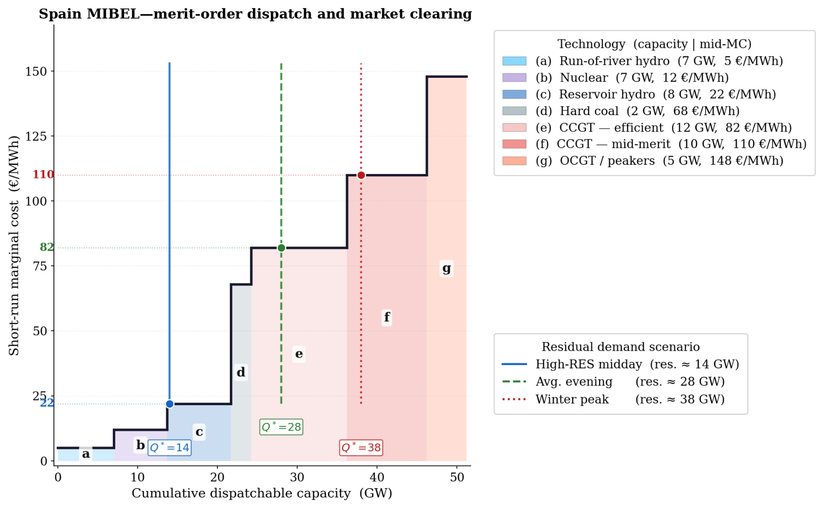
Spain’s electricity market provides a particularly instructive case study. Spain, in fact, operates a marginal-cost-based day-ahead market under the Iberian Energy Market (Mercado Ibérico de Energía, MIBEL) framework, and the clearing price is set by the marginal generator in each hourly auction (i.e., the last accepted unit, at the given marginal cost). Under normal conditions, gas-fired combined-cycle gas turbines (CCGTs) frequently occupy this marginal position, as they offer the highest variable costs among the dispatchable technologies.

This market structure has become increasingly important as the penetration of renewable energy started to accelerate exponentially. According to Red Eléctrica (Alcobendas, Spain), the Technical System Operator in Spain, renewable generation accounted for 42%, 50.3%, and 56.8% of Spain’s national electricity production in 2022, 2023, and 2024, respectively. The Iberian merit order is increasingly characterised by a large block of low-marginal-cost wind, solar, and hydro generation, with CCGTs and open-cycle gas turbines (OCGTs) often acting as swing technologies and, in many hours, as key determinants of the market-clearing price under normal and high-demand conditions [4,5]. It is worth noting that, although hard coal is shown in the merit-order schematic for completeness, coal-fired generation has been almost entirely phased out of the Spanish system since 2020–2021, with the remaining units retired by 2025; coal therefore plays a marginal role in the period covered by this study.

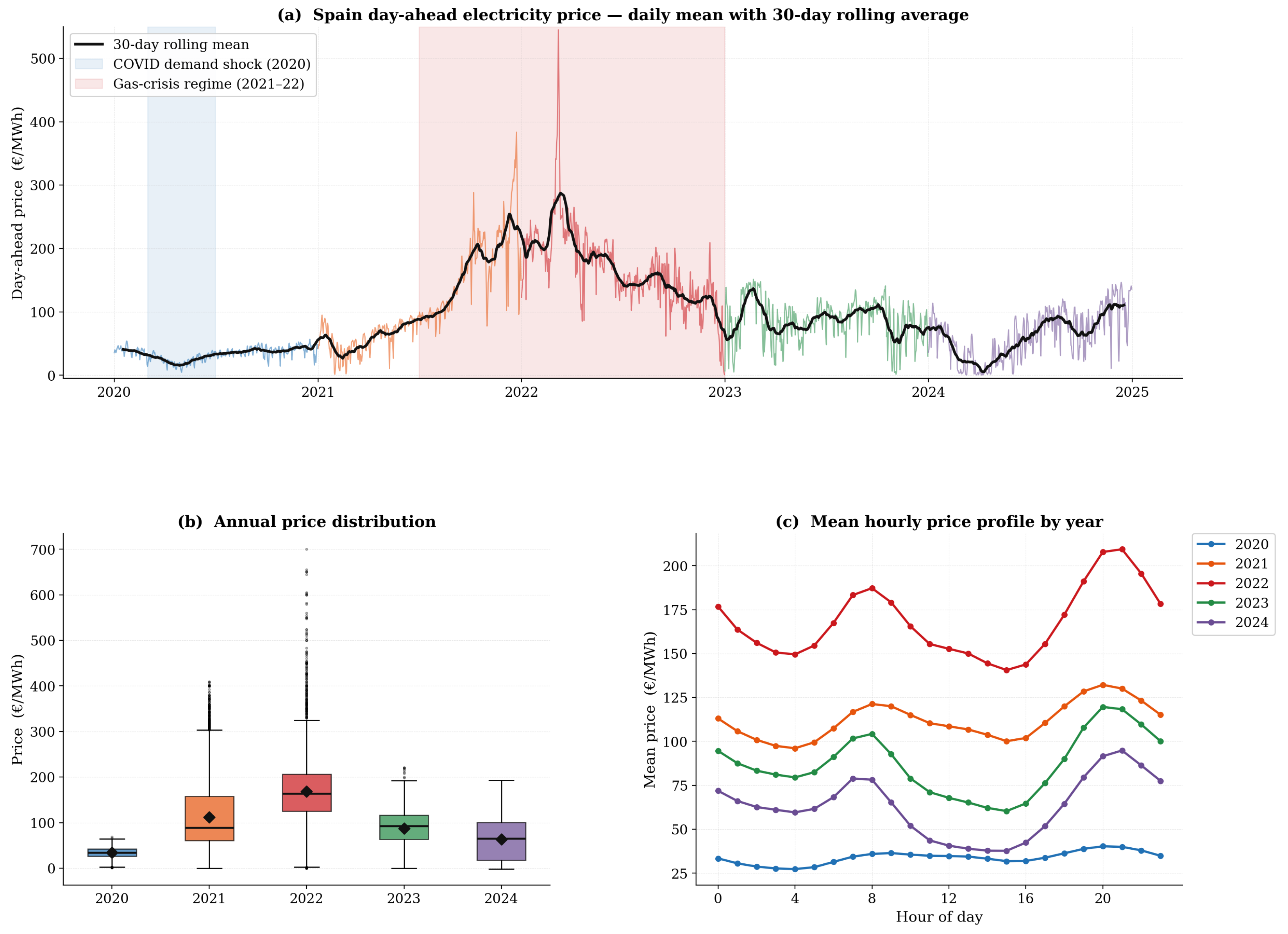
This market structure links Spanish wholesale prices to external fuel-price shocks, especially in periods when gas-fired thermal units frequently set the marginal price, although the strength of this link varies over time with renewable output, hydro conditions, and interconnection flows. That sensitivity became particularly evident during the gas-price crisis of late 2021 and 2022, when the surge in international natural-gas prices following the outbreak of the Russia–Ukraine conflict was rapidly transmitted to wholesale electricity prices [6]. Average Spanish wholesale prices in Q4 2021 exceeded 200 €/MWh, more than three times the Q4 2018 level, and hourly prices in March 2022 reached values as high as 700 €/MWh [5,6]. More recent disruptions to global LNG flows—notably the 2026 Strait of Hormuz crisis, which removed close to 20% of global LNG supply from the market and pushed European wholesale gas prices to their highest levels since early 2023 [7]—are a further reminder of the continued exposure of gas-dependent European power markets to LNG supply shocks, even though Spain’s high renewable share and large regasification capacity provide partial insulation. As such episodes post-date the 2020–2025 sample analysed here, they are noted only as contextual motivation rather than as evidence within this study. Such episodes highlight both the economic relevance and the intrinsic difficulty of electricity price forecasting in Spain, particularly at the week-ahead horizon, where models must remain informative under structurally different and highly volatile market conditions.

With this scenario in mind, the present manuscript investigates week-ahead electricity price forecasting in Spain’s day-ahead market with two complementary aims. First, it benchmarks a set of statistical, machine-learning, and deep-learning models under a common rolling-origin evaluation protocol. Second, it examines how forecast performance is shaped by exogenous drivers that can be interpreted through the Iberian merit-order mechanism, with particular attention to the roles of thermal generation, renewable output, and weather conditions.

The contribution of the paper therefore extends beyond a pure forecasting comparison. The novelty does not lie in the forecasting models, which are standard, nor in the feature-ablation technique, which is common in machine learning, but in their application to the MIBEL week-ahead problem under a leakage-controlled protocol and, above all, in the economic interpretation of the resulting feature importance through the merit-order mechanism. More specifically, the study brings together five elements that are usually addressed separately in the literature: (i) a statistical characterisation of the 2020–2024 Spanish day-ahead price series; (ii) a benchmark comparison of nine forecasting models under a common rolling-origin protocol; (iii) an AOI/LOO analysis of the contribution of key exogenous variables; (iv) a controlled comparison of alternative weather-input scenarios; and (v) a rolling backtest of a battery arbitrage strategy under 24 h and 168 h receding-horizon optimisation.

The remainder of the paper is organised as follows. Section 2 introduces the microeconomics of marginal pricing and discusses the role of gas-fired generation in setting the clearing price, while Section 3 surveys the relevant EPF literature. The 2020–2024 Spain day-ahead price series is then characterised in Section 4, and Section 5 describes the data sources and the preparation steps used in the rest of the paper. 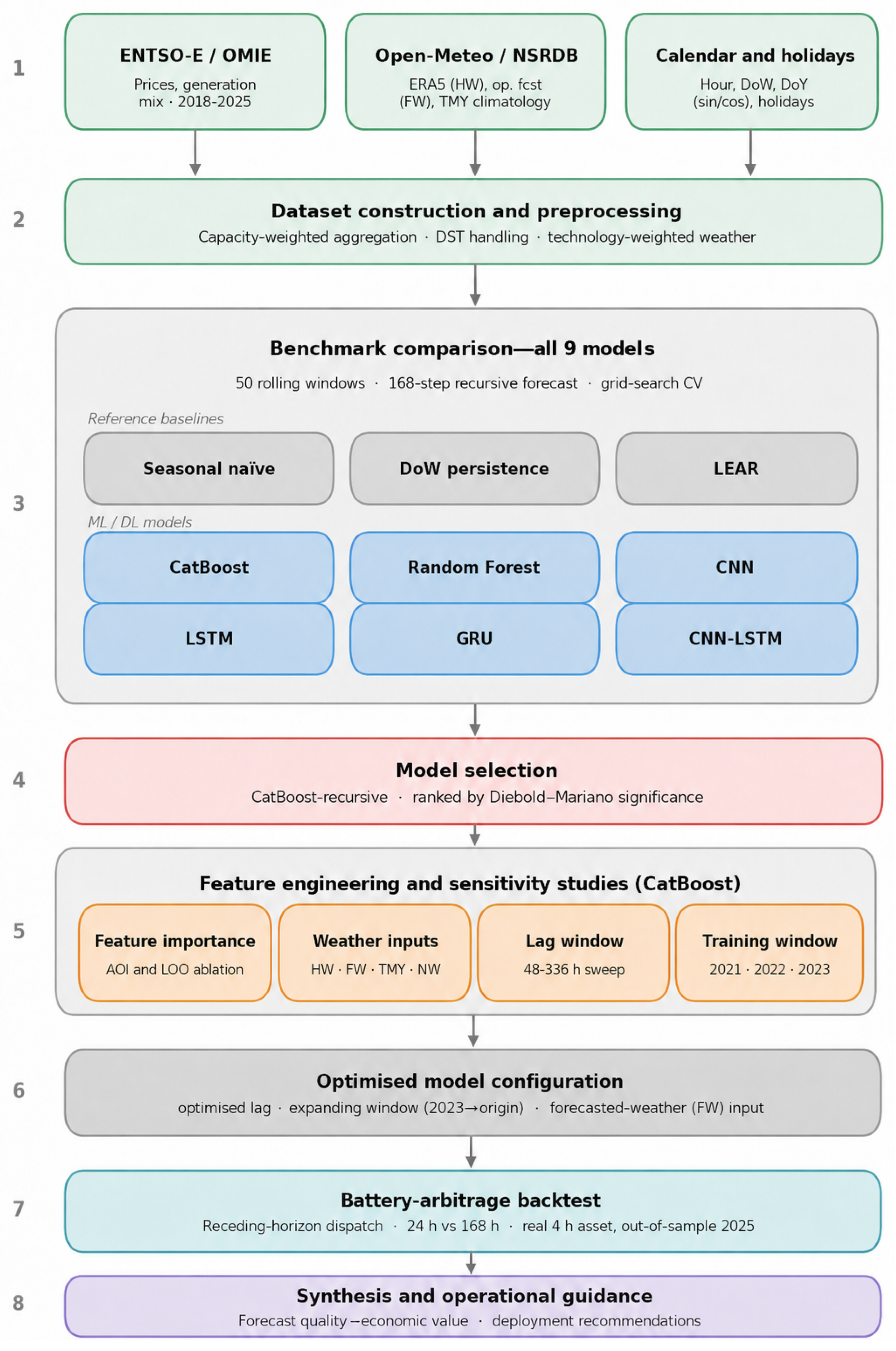Section 6 sets out the eight-stage pipeline together with the model architectures and the evaluation protocol adopted. The forecasting results themselves are reported in Section 7, and Section 8 presents the battery-arbitrage backtest. Section 9 interprets the combined findings, Section 10 discusses the scope of the study and its main limitations, and Section 11 concludes the paper with practical guidance and future research directions.

2. Electricity Price Formation: Marginal-Cost Theory and the Role of Gas

2.1. Merit-Order Dispatch and Marginal Pricing

In competitive wholesale electricity markets, the market-clearing price emerges from the intersection of the supply-offer stack, ranked in ascending order of generators’ marginal costs (the merit order), and relatively inelastic demand [8,9]. All accepted generators receive this uniform clearing price regardless of their individual offer price—a property known as pay-as-cleared or uniform pricing. The generator whose offer defines this intersection is called the marginal unit.

Figure 1 illustrates the merit-order supply stack. Nuclear, run-of-river hydro, wind, and solar PV offer at near-zero marginal cost and are dispatched first. Hard coal and lignite follow, and finally CCGTs and OCGTs—whose variable costs are dominated by the cost of natural gas and CO₂ allowances—are dispatched last [4,10].

Figure 1 illustrates three representative operating states. The stepped supply curve ranks technologies in ascending order of short-run marginal cost; each step width equals available dispatchable capacity (GW). Wind and solar output is subtracted from total demand to obtain the residual demand, shown as three vertical lines. At high-RES midday (residual ≈ 14 GW), reservoir hydro is marginal, $P^{\ast }=22$ €/MWh. At an average evening (residual ≈ 28 GW), an efficient CCGT is marginal, $P^{\ast }=82$ €/MWh. At a winter peak (residual ≈ 38 GW), a mid-merit CCGT is marginal, $P^{\ast }=110$ €/MWh. These three scenarios illustrate why gas-fired CCGT units determine the clearing price for the majority of hours, making gas prices the primary driver of electricity price forecasting error.

2.2. Why Gas-Fired Generation Often Sets the Marginal Price

In Spain’s day-ahead market, low-variable-cost technologies such as nuclear, wind, solar, and run-of-river hydro are typically dispatched before thermal generation. As residual demand increases, gas-fired combined-cycle gas turbines (CCGTs) often move to the margin and therefore frequently determine the market-clearing price under normal system conditions. In the standard merit-order framework, the clearing price is approximated by the short-run marginal cost of the marginal unit [8,9]. For a marginal CCGT plant, and abstracting from relatively small variable O&M costs, this can be written as

$$P^{\ast }\approx {\displaystyle \frac{p_{\mathrm{gas}}}{{\eta }_{\mathrm{CCGT}}}}+p_{{\mathrm{CO}}_2}{e}_{\mathrm{CCGT}},$$

(1)

where $p_{\mathrm{gas}}$ is the natural-gas price (EUR/MWh_th), ${\eta }_{\mathrm{CCGT}}$ is the net electrical efficiency of the plant, $p_{{\mathrm{CO}}_2}$ is the EU ETS carbon price (EUR/tCO₂), and $e_{\mathrm{CCGT}}$ is the specific emissions factor (tCO₂/MWh_el). Typical values for modern CCGTs are ${\eta }_{\mathrm{CCGT}}\approx 0.55$–0.60 and $e_{\mathrm{CCGT}}\approx 0.35$ tCO₂/MWh_el [10,12]. When OCGTs are marginal instead of CCGTs, the corresponding lower efficiency and higher specific emissions are substituted in Equation (1), yielding a higher implied $P^{\ast }$ for the same fuel and carbon prices.

For illustration, with $p_{\mathrm{gas}}=25$ EUR/MWh_th and $p_{{\mathrm{CO}}_2}=55$ EUR/tCO₂, Equation (1) implies $P^{\ast }\approx 61$–65 €/MWh, depending on the assumed efficiency. This is close to the 2024 average price level in the dataset used here and is representative of many non-crisis hours in which gas-fired units set the clearing price. During the 2022 gas crisis, by contrast, natural-gas prices rose to around 130 EUR/MWh_th, pushing the implied marginal cost well above 200 €/MWh through the same mechanism.

This relationship should be interpreted as a stylised approximation rather than an exact hourly pricing rule, since gas-fired units do not set the price in every hour, especially during periods of very high renewable output or very low demand. Even so, because CCGTs frequently determine the clearing price in normal and tight system conditions, gas-related variables provide a strong economic signal for electricity price forecasting.

2.3. Implications for Electricity Price Forecasting

Equation (1) has a direct implication for EPF: the share of gas-fired generation provides the best indicator of the position of the clearing price on the merit-order curve. When the share of gas-fired output is high, residual demand after low-marginal-cost renewable and nuclear generation is also high, so the clearing price is more likely to be set on the steep upper section of the supply stack, where scarcity effects become more pronounced [8]. Conversely, when the share of gas-fired output is close to zero, renewable generation is typically sufficient to satisfy demand at the margin, so the clearing price remains on the flatter inframarginal section and may fall towards zero or even become negative [13].

This mechanism is consistent with the empirical finding discussed in Section 7, that removing natural gas generation from the feature set increases the AOI MAE by 10.55 €/MWh, more than any other individual variable. To the authors’ knowledge, few EPF studies have explicitly linked feature-importance rankings from AOI/LOO analysis to the merit-order pricing mechanism. The practical implication is that gas-fired generation contains highly informative real-time information about the market state, allowing the forecasting model to capture much of the dispatch-driven price formation without explicitly solving the market-clearing optimisation problem.

3. Literature Survey on Short-Term Electricity Price Forecasting

3.1. Forecasting Models and Horizons

Early EPF research relied mainly on statistical time-series methods such as the autoregressive moving average (ARMA) and autoregressive integrated moving average (ARIMA) families—which model the current price as a linear combination of past prices and past forecast errors [14] — together with regime-switching extensions that allow the model coefficients to vary across distinct market states. These approaches capture daily and weekly seasonality through relatively simple linear dynamics [2]. However, as electricity markets became more exposed to renewable generation, fuel-price shocks, and other non-linear drivers, the limitations of purely linear specifications became more evident, particularly during volatile and regime-changing periods [2]. In a widely cited review, Weron (2014) [2] grouped electricity price models into five broad categories: multi-agent, fundamental, reduced-form, statistical, and computational-intelligence models. Within short-term forecasting, computational-intelligence approaches based on machine learning and deep learning have since become the dominant paradigm. Among these, kernel-based methods such as support vector machines (SVMs) [15] and sparsity-inducing regularised regressions such as the least absolute shrinkage and selection operator (LASSO) [16]—which shrinks small coefficients toward zero to perform automatic variable selection—have served as influential baselines and underpin more recent benchmarks such as LEAR.

A key statistical benchmark is the Lasso-estimated auto-regressive (LEAR) model [3], a high-dimensional linear autoregressive specification in which coefficients are estimated using LASSO regularisation. Its main strengths are interpretability, computational efficiency, and the ability to perform variable selection in large lagged feature spaces. Lago et al. [3] introduced LEAR as an open-access benchmark in a large comparison across several European markets, showing that it remains competitive with neural networks for 24-hour-ahead forecasting, although its linear structure can limit performance under strong non-linearities.

Among machine-learning methods, gradient-boosted decision trees (GBDTs) are particularly attractive because they combine high predictive accuracy with fast training and the ability to handle heterogeneous tabular inputs [17,18]. Wu et al. (2022) [19] reported that a PSO-optimised XGBoost model outperformed SVM, LSTM, and ARIMA for the Australian market. CatBoost has been used less frequently in EPF, but Yıldız (2023) [20] found it to outperform ridge regression, gradient boosting, and SVM in the Turkish market. Loizidis et al. (2024) [21] likewise showed that tree-based methods achieved the lowest errors among eight models in German and Finnish markets. Earlier, Ludwig et al. (2015) [22] had already established Random Forest as a strong 24-hour-ahead benchmark for the German market. Among tree-based methods, Random Forest appears in prior MIBEL studies, whereas CatBoost has not been benchmarked as a standalone forecaster in the MIBEL studies reviewed here; accordingly, the present study includes RF as an established benchmark and CatBoost as a strong modern boosting candidate.

Deep-learning models have also received substantial attention, especially LSTM, GRU, CNN, and hybrid CNN–LSTM architectures [23,24,25]. For Spain, Hernández et al. (2023) [26] reported that LSTM and GRU outperform statistical baselines. More recently, Failing et al. (2026) [27] benchmarked feedforward, LSTM, and Conv1D architectures on day-ahead spot prices in the Spanish market, confirming the importance of variable selection and reporting rMAE of 13.29% over an 184-day test period; their work complements the present study, which targets the week-ahead horizon and evaluates forecast value through an operational battery-arbitrage backtest rather than purely accuracy-based metrics. Hybrid CNN–LSTM models are particularly appealing because they combine convolutional layers for local pattern extraction with recurrent layers for sequential dependence modelling.

Prior work has shown that CNN–LSTM architectures can outperform standalone LSTMs in electricity-price forecasting settings [28], while Abdellatif et al. (2024) [29] further enhanced a CNN-BiLSTM structure with an autoregressive bypass in the Nordic market. Recent work has also emphasised collaborative and operational forecasting frameworks for day-ahead electricity prices, highlighting the value of model design choices beyond raw predictive accuracy [30].

Taken together, the literature suggests that no single model class dominates in all settings: linear benchmarks such as LEAR remain competitive, tree-based methods are strong on structured tabular inputs, and deep-learning models can be advantageous when temporal and non-linear dependencies are strong. In the benchmark presented here, CNN–LSTM outperforms the standalone deep-learning architectures in mean error, while CatBoost remains highly competitive and is preferred operationally because of its greater consistency and much lower retraining cost.

3.2. Forecasting Evidence for the MIBEL/Spain Market

The MIBEL market has attracted a dedicated stream of EPF research, summarised in Table 1. Several structural features distinguish MIBEL from other European markets and make it a demanding forecasting testbed: the high share of intermittent renewables (approaching 50% by 2023 [31]), the marginal pricing mechanism described in Section 2, and the occurrence of distinct non-stationary periods—including the including the 2016–2017 CCGT scheduling episode investigated by the CNMC [32,33], the COVID-19 demand shock in the Iberian market (2020) [34], and the gas-price crisis (2021–2022).

The earliest competitive ML studies for MIBEL used shallow neural networks: Catalão et al. (2007) [35] demonstrated that a wavelet-transform neural hybrid (NNWT) outperformed ARIMA and feedforward networks on the 168-hour-ahead horizon. Monteiro et al. (2016) [36] extended this line of work to MIBEL day-ahead and intraday sessions with MLP-based DSMPF/ISMPF models, systematically testing combinations of demand, generation, weather, and lagged-price inputs to identify the most informative exogenous variables for each session.

The introduction of tree-based methods represented a step change: Andrade and Bessa (2017) [37] reported MAE = 3.03 €/MWh and RMSE = 4.04 €/MWh for a gradient-boosted trees model on MIBEL (2015–2017), using a rolling 550-iteration window with Bayesian hyperparameter optimisation. A distinctive contribution was the rescaling of hourly GBT predictions with a daily linear quantile regression, which reduced systematic bias. Romero et al. (2019) [38] obtained comparable accuracy (MAE = 3.92–4.50 €/MWh) with Random Forest using 24-h lagged prices, wind/solar generation, demand, and French interconnection prices, and concluded that target-variable normalisation strategy significantly affected validation accuracy. For the Spanish market specifically, Díaz et al. (2019) [39] combined machine-learning regression with an explanatory analysis of day-ahead price formation, showing that predictive and interpretive objectives can be studied jointly.

Ferreira et al. (2019) [40] extended the analysis to the medium-term horizon, showing that MLR with fundamental market variables achieved MAPE = 6.45% for Spain in 2018, underscoring the continued relevance of linear methods at longer horizons. Vega-Márquez et al. (2021) [41] presented a methodologically rigorous comparison of LSTM, CNN, TCN, MLP, decision trees, and RF across three distinct market sub-periods (normal, COVID quarantine, and alleged fraud), reporting LSTM and CNN tied for best accuracy (MAE = 3.54 €/MWh, LSTM) and concluding that model rankings are period-dependent—a finding with direct implications for training-window selection. Leal et al. (2023) [42] benchmarked FFNN and LSTM over the 2015–2019 MIBEL period and reported competitive performance at both 1-day and 5-day horizons, with 5-day MAPEs in the 6.84–8.82% range. This is therefore a useful Iberian reference for multi-step EPF, even though its main objective was to study how increasing renewable penetration may affect future price formation rather than to provide a broad market-wide benchmark study.

Table 1 consolidates representative day-ahead EPF studies, covering MIBEL/Spain (upper block), CatBoost and GBDT studies across markets (middle block), and selected cross-market DL comparisons (lower block). Columns report models compared, forecast horizon, data period, exogenous features used, lag structure, and hyperparameter optimisation method. Error metrics are deliberately omitted from the table because they are not directly comparable across markets, price levels, test periods, and horizons; the discussion below focuses instead on methodological dimensions.

Table 1. Representative EPF studies. Upper block: Spain/MIBEL; middle block: tree-based models in other markets; lower block: cross-market DL benchmarks. Horizon abbreviations: DA = day-ahead (24 h); W = week-ahead (168 h); MT = medium-term; ID = intraday. “—” = not reported.

Study (Year)	Models Tested	Horiz./Data Period	Exogenous Features	Lag Structure	HP Optimisation
MIBEL/Spain point-forecast studies
Catalão et al. [35] (2007)	NNWT, ARIMA, WNN, FNN	W/Spain 2002	None (univariate price)	Four of six prior weeks	Trial-and-error (hidden units)
Monteiro et al. [36] (2016)	DSMPF, ISMPF (MLP variants)	DA/ID/Spain 2012–2013	Demand, generation, weather, past prices	Day D and Day D−6 prices	Variable selection; averaging over 20 runs
Andrade & Bessa [37] (2017)	GBT, LQR	DA/Spain 2015–2017	Futures price, wind penetration, load forecasts	Rolling price lags	Bayesian optimisation; rolling window
Ferreira et al. [40] (2019)	MLR	MT/Spain 2017–2018	Generation, demand, interconnections	—	—
Romero et al. [38] (2019)	Ridge, KNN, SVR, MLP, RF	DA/Spain 2014–2017	Wind/solar, demand, imports/exports, weather, French price	24, 48, 72 h lags	Grid search; normaliser comparison
Vega-Márquez et al. [41] (2021)	LSTM, CNN, TCN, MLP, Trees, RF	DA/Spain 2016–2020	None (univariate price)	Optimised history window (MIMO)	Grid search across three market sub-periods
Hernández et al. [26] (2023)	LR, RF, XGBoost, LSTM, GRU	DA/Spain (n.r.)	Price history, demand	Standard RNN sequences	No explicit tuning reported
tree-based evidence in other markets
Ludwig et al. [22] (2015)	AR, ARMA, LASSO, RF	DA/Germany	Historical prices, weather variables	24 h and 168 h	Feature selection with LASSO/RF
Wu et al. [19] (2022)	PSO-XGBoost, SVM, LSTM, ARIMA	DA/Australia (NEM) 2018–2021	Demand, generation mix, temperature	PSO-selected lag window	PSO over XGBoost hyperparameters
Yıldız [20] (2023)	LR, Ridge, GB, SVM, CatBoost	DA/Turkey 2020–2022	Gas price, load forecast, past prices	Not reported; EMD preprocessing	No formal HPO reported
Loizidis et al. [21] (2024)	ELM, ANN, RF, XGBoost	DA/Germany/Finland 2019–2022	Production–consumption balance and market inputs	Daily class-specific setup	Bootstrap across price regimes
Broader benchmark and deep-learning comparisons
Lago et al. [3] (2021)	LEAR, DNN, CNN, LSTM, and 11 others	DA/EPEX, Nord Pool, OMIE 2013–2018	Prices, load, generation (market-dependent)	24, 48, 168 h	Open benchmark; rolling window
Abdellatif et al. [29] (2024)	CNN, LSTM, CNN-BiLSTM, CNN-BiLSTM-AR	DA/Nordic market	Price history	Sequences up to 168 h	GA, PSO, random-search HPO; stat. testing
Das & Schlüter [43] (2025)	R-NP	DA/Germany 2021–2024	Exogenous fundamentals, regime indicators	Rolling window	Regime detection + non-parametric fitting

Note: The best-performing model(s) per study are shown in bold in the Models Tested column.

Table 1. Representative EPF studies. Upper block: Spain/MIBEL; middle block: tree-based models in other markets; lower block: cross-market DL benchmarks. Horizon abbreviations: DA = day-ahead (24 h); W = week-ahead (168 h); MT = medium-term; ID = intraday. “—” = not reported.

Study (Year)	Models Tested	Horiz./Data Period	Exogenous Features	Lag Structure	HP Optimisation
MIBEL/Spain point-forecast studies
Catalão et al. [35] (2007)	NNWT, ARIMA, WNN, FNN	W/Spain 2002	None (univariate price)	Four of six prior weeks	Trial-and-error (hidden units)
Monteiro et al. [36] (2016)	DSMPF, ISMPF (MLP variants)	DA/ID/Spain 2012–2013	Demand, generation, weather, past prices	Day D and Day D−6 prices	Variable selection; averaging over 20 runs
Andrade & Bessa [37] (2017)	GBT, LQR	DA/Spain 2015–2017	Futures price, wind penetration, load forecasts	Rolling price lags	Bayesian optimisation; rolling window
Ferreira et al. [40] (2019)	MLR	MT/Spain 2017–2018	Generation, demand, interconnections	—	—
Romero et al. [38] (2019)	Ridge, KNN, SVR, MLP, RF	DA/Spain 2014–2017	Wind/solar, demand, imports/exports, weather, French price	24, 48, 72 h lags	Grid search; normaliser comparison
Vega-Márquez et al. [41] (2021)	LSTM, CNN, TCN, MLP, Trees, RF	DA/Spain 2016–2020	None (univariate price)	Optimised history window (MIMO)	Grid search across three market sub-periods
Hernández et al. [26] (2023)	LR, RF, XGBoost, LSTM, GRU	DA/Spain (n.r.)	Price history, demand	Standard RNN sequences	No explicit tuning reported
tree-based evidence in other markets
Ludwig et al. [22] (2015)	AR, ARMA, LASSO, RF	DA/Germany	Historical prices, weather variables	24 h and 168 h	Feature selection with LASSO/RF
Wu et al. [19] (2022)	PSO-XGBoost, SVM, LSTM, ARIMA	DA/Australia (NEM) 2018–2021	Demand, generation mix, temperature	PSO-selected lag window	PSO over XGBoost hyperparameters
Yıldız [20] (2023)	LR, Ridge, GB, SVM, CatBoost	DA/Turkey 2020–2022	Gas price, load forecast, past prices	Not reported; EMD preprocessing	No formal HPO reported
Loizidis et al. [21] (2024)	ELM, ANN, RF, XGBoost	DA/Germany/Finland 2019–2022	Production–consumption balance and market inputs	Daily class-specific setup	Bootstrap across price regimes
Broader benchmark and deep-learning comparisons
Lago et al. [3] (2021)	LEAR, DNN, CNN, LSTM, and 11 others	DA/EPEX, Nord Pool, OMIE 2013–2018	Prices, load, generation (market-dependent)	24, 48, 168 h	Open benchmark; rolling window
Abdellatif et al. [29] (2024)	CNN, LSTM, CNN-BiLSTM, CNN-BiLSTM-AR	DA/Nordic market	Price history	Sequences up to 168 h	GA, PSO, random-search HPO; stat. testing
Das & Schlüter [43] (2025)	R-NP	DA/Germany 2021–2024	Exogenous fundamentals, regime indicators	Rolling window	Regime detection + non-parametric fitting

Note: The best-performing model(s) per study are shown in bold in the Models Tested column.

An analysis of Table 1 reveals the following areas in need of further research. The present paper addresses these to advance the body of literature on the topic:

1.

Week-ahead forecasting is substantially less explored in the Iberian literature than day-ahead forecasting, especially for Spain under post-2021 market conditions. Catalão et al. (2007) [35] considered a 168-h horizon with a simple univariate NNWT model on 2002 data, and de Marcos et al. [44] explicitly considered both one-day and one-week horizons in a hybrid Iberian framework. However, these studies predate both today’s renewable penetration levels and the 2021–2022 gas-price crisis, leaving a gap that is very important from a practical standpoint under current market conditions for storage operations and fuel-procurement scheduling.

2.

Despite CatBoost’s documented superiority in the Turkish market [20] and its strong performance in tabular ML benchmarks [45], it has not, to the authors’ knowledge, been systematically benchmarked on the Iberian market. The MIBEL context is structurally different from Turkey and other European markets due to its specific renewable mix, the marginal pricing role of CCGT plants, and the Iberian exception mechanism implemented in 2022.

3.

To the authors’ knowledge, none of the MIBEL studies in Table 1 include the 2021–2022 gas-price crisis in their training or test data—the most challenging and economically consequential period for electricity market participants in recent history. Studies that do cover a crisis period (e.g., Das and Schlüter [43] for Germany) treat it as an external phenomenon rather than quantifying its impact on forecast error through a controlled backtest spanning 2020–2024.

4.

Feature selection and explanatory-variable analysis are not absent from the MIBEL literature: Monteiro et al. [36], Andrade and Bessa [37], Romero et al. [38], and Díaz et al. [39] all provide evidence on informative predictors. The gap addressed here is narrower but still important: a formal AOI/LOO ablation experiment interpreted explicitly through the merit-order marginal-pricing mechanism, linking the relative importance of natural gas generation to its theoretical role as the marginal unit under Equation (1).

5.

The MIBEL studies reviewed here generally use fixed lag structures—typically the 24, 48, or 168-h lookbacks recommended by Weron [2]—and no study in this literature appears to investigate whether the optimal lag window varies with forecast day (Day 1 vs. Day 7). The sweep performed here over 48–384 h reveals that the optimal lag increases from 96 h for Day 1 to 384 h for Day 7, a practically important finding for designing recursive forecasting systems.

6.

To the authors’ knowledge, no study in the MIBEL literature reviewed here compares all four of these weather-data choices (HW, FW, TMY, and a no-weather baseline) under identical model conditions. This comparison is practically important for operators who must decide which weather data source to use operationally.

7.

While multi-horizon electricity-price forecasting and value-oriented trading evaluation are already present in the broader literature [46,47], the present study contributes a Spain-focused benchmark for hourly week-ahead forecasting under recent market regimes, and evaluates forecast usefulness through a battery-arbitrage backtest under both 24 h and 168 h rolling optimisation horizons. This is complemented by an AOI/LOO analysis that interprets feature importance through the Iberian merit-order mechanism.

3.3. Feature Engineering and Exogenous Variables

The choice of input features is critical for EPF accuracy. Weron [2] and Ziel and Steinert [48] recommend including lagged prices, calendar features, and fundamental variables (load, generation by type). Several studies have shown the importance of fuel prices and generation mix [1,49]. Cludius et al. [13] further show, in the German market, how wind and photovoltaic output can depress spot prices through the merit-order effect. For MIBEL specifically, Andrade and Bessa [37] included wind penetration and load forecasts in their GBT model, finding these to be among the most informative inputs. Romero et al. [38] confirmed that adding French interconnection prices improves MIBEL accuracy. The present work formally quantifies the marginal contribution of each generation-type feature through AOI/LOO analysis and interprets the ranking through merit-order pricing theory, with natural gas generation acting as a direct proxy for price-setting thermal dispatch in many hours.

3.4. Probabilistic Forecasting for MIBEL

While point forecasts are the focus of this paper, the probabilistic EPF literature is rapidly evolving and directly relevant to risk management in MIBEL. Andrade and Bessa [37] appended a linear quantile regression (LQR) to their GBT model, achieving CRPS = 1.22% with calibration deviation below 7% for 2015–2017 MIBEL data. Uniejewski (2025) [50] introduced smoothing quantile regression (SQR) averaging, evaluated on EPEX and Spanish OMIE data (2015–2023), showing that SQR averaging outperforms standard QRA and all benchmarks on the Pinball score. The probabilistic methods of Nowotarski and Weron [51] that uses quantile regression averaging over a pool of point models, remain an influential baseline. Integrating such probabilistic wrappers around the CatBoost model developed here represents a natural extension for future work.

4. Statistical Analysis of the Spain Day-Ahead Price Series (2020–2024)

The experimental layers of the study span different time periods, as summarised in

Table 2. Temporal scope of each experimental layer.

Layer	Period	Purpose
Raw source data	2018–2025	Data gathered for the subsequent analysis;
Price-series analysis	2020–2024	Statistical characterisation of regimes;
Retrospective backtest	2019–2024 (50 origins/yr)	Historical error evolution, each window being forecasted trains on data starting on the previous year and up to the forecasted window;
Common benchmark (training)	from 2023	Equal-conditions model comparison;
Validation (forecast)	2024 (50 rolling origins)	Forecast evaluation and model selection;
Out-of-sample test	2025	Held-out generalisation check.

. This separation is intentional: the raw data period is wider than the statistical-analysis window; the common benchmark trains from 2023 and is validated on 50 weekly rolling origins in 2024, with 2025 held out entirely as an out-of-sample test, while the retrospective backtest extends back to 2019 to capture the full pre-crisis baseline.

4.1. Price Regimes and Annual Statistics

Figure 2 presents an overview of the Spain DA hourly price series from 2020 to 2024. The data (43,848 hourly observations, reflecting two leap years, 2020 and 2024) reveal three distinct market regimes: (i) a stable pre-crisis period (2020–mid-2021) with annual mean prices of 33.9 and 111.9 €/MWh for 2020 and 2021 respectively; (ii) a gas-crisis regime (mid-2021 to end-2022) with annual mean 167.5 €/MWh and a single-hour maximum of 700 €/MWh in March 2022; and (iii) a post-crisis normalisation (2023–2024) with declining means of 87.1 and 63.0 €/MWh. The COVID-19 demand shock of spring 2020 produced a transient price dip (annual mean 33.9 €/MWh) consistent with the demand-driven price transmission documented by Pereira da Silva et al. [52].

Figure 2b highlights the dramatic increase in the interquartile range and upper whisker during 2021–2022, confirming that the gas crisis increased not only the level but also the spread of the price distribution—a classical “fat-tail” behaviour [2]. Figure 2c shows that intra-day profiles evolved substantially: the characteristic solar-driven midday dip, barely visible in 2020, deepened through 2023–2024 as utility-scale photovoltaic capacity grew.

4.2. Volatility Dynamics, Distribution, and Forecast Error Link

Figure 3 presents a two-panel statistical characterisation. Panel (a) shows a level-based realised volatility, defined as the 30-day rolling standard deviation of the daily mean price (in €/MWh):

$${\sigma }_t=\mathrm{std}\left\{P_d:d\in [t-29,t]\right\},$$

(2)

where $P_d$ is the daily mean price. This estimator peaks in March 2022 (≈103 €/MWh) at the height of the gas crisis, and is much smoother than a short-window return-based estimator. The same measure is used later for the regime statistics and for the volatility–error relationship discussed in Section 7.3, so that a single volatility definition is used throughout. We note separately that a return-based volatility (annualised standard deviation of daily log-returns) behaves differently: it is dominated by near-zero prices and therefore peaks not in 2022 but in 2023–2025 (e.g., 34 days with a daily-mean price below 5 €/MWh in 2024, versus a single such day in 2022), reflecting the growing incidence of renewable-surplus hours that flatten the merit-order curve near zero rather than a high-price crisis. Panel (b) presents kernel density estimates of the hourly price distribution for each year. The 2020 distribution is tightly concentrated near 30–40 €/MWh, reflecting stable pre-crisis conditions. The 2021–2022 distributions shift markedly rightward and flatten, with 2022 exhibiting a pronounced heavy right tail extending beyond 400 €/MWh, a classical “fat-tail” behaviour associated with scarcity pricing when gas plants operate as price setters near capacity [2]. By 2024 the distributions return toward lower price levels, and a secondary mass appears near zero, consistent with the partial market normalisation and rising renewable share described in Section 4. The link between elevated volatility and forecast error is quantified empirically in Section 7.3 and Section 7.4: the 2022 training window inflates the 2024 MAE by 12.85%, directly reflecting the non-representative statistical regime of that year.

The hourly price series exhibits strong autocorrelation at multiples of 24 h (daily periodicity driven by demand cycles) and a secondary weekly peak near 168 h, with ACF values at these lags well above the 95% confidence interval (±1.96/$\sqrt{n}$). These autocorrelation properties directly motivate the use of lag features in the forecasting model; in particular, the persistence at 168 h justifies the chosen 336-h lag window (two full weekly cycles) that will be seen in Section 7.8. Intra-day and intra-week price patterns are also evident: prices are systematically lower on weekends (reduced industrial demand) and show characteristic morning and evening peaks on weekday, that is a structural features that the model’s cyclical time encoding must capture [2].

5. Spain’s Electricity Market and Data Description

5.1. Market Structure and Design

Spain’s wholesale electricity market operates within the MIBEL framework (Mercado Ibérico de Energía, Iberian Electricity Market) [53]. The Comisión Nacional de los Mercados y la Competencia (CNMC, National Commission for Markets and Competition) supervises the functioning and degree of competition of the electricity market, while OMIE (Operador del Mercado Ibérico de Energía, Iberian Energy Market Operator) operates the day-ahead and intraday auctions [11]. The market operates as a day-ahead market (DAM) complemented by an intraday market (IDM) for real-time adjustments and a balancing market (BM).

Day-Ahead Market

In the day-ahead session, market participants submit hourly supply offers and demand bids that are aggregated into sale and purchase curves and matched to determine the market-clearing outcome [11]. The auction is held daily at 12:00 CET. All accepted offers receive the uniform clearing price set by the marginal unit. Low-marginal-cost renewables and nuclear typically dispatch inframarginal, capturing scarcity rents when gas-fired units set the marginal price [8,54]. Spain’s coupling with Portugal under MIBEL, and interconnections with France and Morocco, allow cross-border flows to influence the clearing price, although internal supply–demand balance remains dominant [39].

Two regulatory interventions affecting the price series should be noted. First, with the go-live of Single Day-Ahead Coupling (SDAC) interim coupling in June 2021, the previous MIBEL local price bounds of $[0,180.3]$ €/MWh were replaced by the harmonised SDAC bounds $[-500,+3000]$ €/MWh; under the Harmonised Maximum and Minimum Clearing Prices methodology, the upper bound was then raised to $+4000$ €/MWh on 10 May 2022 during the price spike [55]. Second, the Iberian exception (the “tope al gas” mechanism, Royal Decree-Law 10/2022) operated from 15 June 2022 to 31 December 2023, subsidising the fuel cost of gas-fired generation (capped initially at 40 €/MWh and escalating toward 65 €/MWh) and thereby artificially lowering the marginal clearing price [56]. These interventions are relevant context for the descriptive statistics of Section 4. They do not, however, confound the forecasting experiments: as detailed in Section 6, models are trained on a rolling window starting in 2023 and evaluated on 2024–2025, so the 2021 bound change precedes the entire modelling window and the gas cap had expired before the evaluation period, during which gas-fired units again set the marginal price without subsidy.

5.2. Data Sources and Preparation

The dataset used in this work spans from 1 January 2020 to 31 December 2024 (43,848 hourly observations, and 2025 is held as OOS) and includes: Hourly DA prices obtained from OMIE, accessed via the ENTSO-E Transparency Platform [55]. The dataset includes 896 h with zero or negative prices, reflecting renewable surplus events; hourly generation by technology type and total load from the ENTSO-E Transparency Platform [55]. These data are used to derive the natural gas generation feature, the marginal-price proxy identified in Section 2; hour of day, day of week, Spanish bank holiday indicator, and a linear time trend; hourly lags from the past 336 h (two weeks), selected via the lag optimisation study described in Section 7.8; historical, forecast, and Typical Meteorological Year (TMY) weather from OpenMeteo [57] and NSRDB [58], spatially aggregated using generation-capacity weights (see

Table 3. Top five locations for solar PV aggregation (capacity weights, 2023).

Location	Weight (%)
Usagre (Badajoz)	25.09
Puertollano (Ciudad Real)	24.01
Seville (Solúcar Complex)	21.07
Teruel (Rural Area)	9.41
Segovia	7.46

and

Table 4. Top five locations for wind generation aggregation (capacity weights, 2023).

Location	Weight (%)
Burgos	21.55
Zaragoza (Ebro Valley)	17.03
Albacete	15.83
A Coruña	12.62
Tarifa	11.82

). For each variable, regional values are aggregated using technology-specific capacity weights to align meteorological inputs with the spatial distribution of installed generation. Solar-related variables (temperature, precipitation, cloud cover) are aggregated over the principal PV locations:

$$X_{\mathrm{solar}}={\displaystyle \frac{{\sum }_{i=1}^N{X}_i{w}_{i,\mathrm{solar}}}{{\sum }_{i=1}^N{w}_{i,\mathrm{solar}}}},$$

(3)

where $X_{\mathrm{solar}}$ is the aggregated solar-weighted weather variable, $X_i$ is the local value of the variable at location i, $w_{i,\mathrm{solar}}$ is the installed solar PV capacity at location i (used as the aggregation weight), and $N=5$ is the number of locations (Table 3). Wind-related variables are aggregated analogously over the principal wind locations (Table 4), substituting installed wind capacity $w_{i,\mathrm{wind}}$ for the weights:

$$X_{\mathrm{wind}}={\displaystyle \frac{{\sum }_{i=1}^N{X}_i{w}_{i,\mathrm{wind}}}{{\sum }_{i=1}^N{w}_{i,\mathrm{wind}}}}.$$

(4)

The weather variables are aggregated using technology-specific capacity weights in order to align meteorological inputs with the spatial distribution of installed generation capacity, with each site weighted by its 2023 share of installed capacity. This weighting scheme ensures that regions with a larger contribution to aggregate generation exert a proportionally larger influence on the explanatory variables. As a result, the constructed series should better capture the effective weather conditions and avoid noise from less relevant areas.

6. Forecasting Methodology

The methodology adopted in this study follows an eight-stage pipeline, summarised in Figure 4. The first two stages assemble the shared dataset that is used by every model in the comparison. Stages 3 and 4 then benchmark all nine candidate models under identical conditions and identify the best-performing one for further investigation. Stages 5 and 6 optimise the selected model in depth, and the final two stages apply it to a battery-arbitrage backtest and synthesise the combined findings into operational guidance.

The eight stages of the pipeline can be summarised as follows.

• Stage 1: Three parallel data streams are ingested: hourly day-ahead prices and generation by technology from the ENTSO-E and OMIE platforms; weather data from Open-Meteo and NSRDB in three variants (historical ERA5 reanalysis (HW), operational seven-day-ahead numerical forecasts (FW), and Typical Meteorological Year climatology (TMY)) at multiple Spanish locations; and calendar features (hour of day, day of week, day of year encoded as sine/cosine pairs, and Spanish bank holidays).
• Stage 2: The three streams are merged into a single hourly feature matrix. Weather variables are aggregated spatially using production-capacity weights over the five leading PV and wind regions (Table 3 and Table 4). All series are placed on a fixed UTC + 1 (CET, DST-free) hourly grid: at the spring transition the missing hour is forward-filled (in the price series and in the aligned exogenous series), and at the autumn transition the duplicated hour is dropped; weather is mapped to the same clock by a fixed $+1$ h shift before reindexing, so no clock-change discontinuity is introduced. A lag matrix spanning 1 to 384 h is then assembled, with the optimal lag window selected later in Stage 5. Neural-network inputs are standardised, while tree-based models receive raw values.
• Stage 3: Nine candidate models are evaluated under identical conditions on a common endogenous feature set (lagged prices and calendar variables, 168-h lag window); Table 5 maps every feature group to the stage in which it is active. The protocol issues a weekly rolling forecast across the 2024 out-of-sample year, each origin producing 168 consecutive hourly predictions, with the start day of the week rotated from origin to origin so that the result does not depend on a fixed first-day-of-week. For every origin each model is trained on an expanding window of strictly preceding data that begins in 2023 and ends at the origin; all models share the same window at each origin, so the comparison is not confounded by differences in training data. Hyperparameters are tuned by time-series cross-validation that respects temporal order (Table 6). No data earlier than 2023 enter the benchmark. Three reference baselines are included: a Seasonal naïve, a Day-of-Week persistence, and LEAR [3], the state-of-the-art statistical benchmark in EPF [2]. Six machine-learning and deep-learning candidates are then compared: CatBoost, Random Forest, CNN, LSTM, GRU, and the hybrid CNN–LSTM. Two CatBoost multi-step strategies are distinguished in the focused comparison of Section 7.1: a recursive one-step model rolled out 168 h, and a direct multi-horizon model that predicts each day’s prices jointly.
• Stage 4: The nine models are ranked jointly on mean MAE, mean RMSE, and average retraining time. CatBoost-recursive and CNN–LSTM are statistically indistinguishable on endogenous features (MAE ≈ 22.9 €/MWh; Diebold–Mariano $p=0.99$) and retrain in comparable time (about 31 and 33 s per monthly recalibration). The tie is broken in later stages, where CatBoost-recursive extracts more value from the weather signal and is markedly more robust on the held-out 2025 year; both front-runners are therefore carried into the focused comparison, and CatBoost is selected for the subsequent optimisation and application stages.
• Stage 5: Four analyses are then applied to the selected CatBoost model: an add-one-in and leave-one-out feature importance study (Section 7.5 and Section 7.6); a controlled comparison of the four weather scenarios (HW, FW, TMY, and NW) under fixed model and lag settings (Section 7.7); a lag-window sweep from 48 to 384 h per forecast day (Section 7.8); and a training-window sensitivity analysis based on the years 2021, 2022, and 2023 (Section 7.4).
• Stage 6: The findings of Stage 5 converge on a practical optimum: a 336-h lag window, an expanding training window anchored at 2023, and an operational (forecasted) weather input, which is found to be the best-performing weather scenario (Section 7.7). CatBoost is re-tuned under this configuration, yielding the refined error metrics reported later in Section 7.8.
• Stage 7: The forecasts produced by the optimised model are put to economic use in a receding-horizon battery-arbitrage backtest of a 4-h grid-scale unit, run under both 24-h and 168-h optimisation horizons on the held-out 2025 year; the value captured is benchmarked against a perfect-foresight ceiling (Section 8).
• Stage 8: Finally, the fixed configuration is validated out-of-sample: because training always uses an expanding window of strictly past data anchored at 2023, 2024 is evaluated without leakage, and a completely held-out 2025 year (used for nothing during development) provides an independent check. The horizon-wise and regime-stratified error profiles, the feature attribution, and the battery results are then synthesised into practical guidance for week-ahead forecasting in MIBEL.

Table 5. Feature groups active at each stage of the workflow. √ = included; — = not used. The weather-scenario study evaluates the no-weather (NW), forecasted-weather (FW), TMY, and historical-weather (HW) inputs as separate single-weather arms on a fixed model. “Known at issuance” indicates whether a group is available when a week-ahead forecast is made; the two ex-post groups are confined to the explanatory feature-importance analysis.

Feature Group	Screening Benchmark Section 7.1	AOI/LOO Importance Section 7.6	Weather Study Section 7.7	Operational Fcst and Battery Section 8	Known at Issuance
Lagged DA prices	√	√	√	√	Yes
Calendar features	√	√	√	√	Yes
Forecast weather	—	—	√	√	Yes
TMY climatology	—	—	√	—	Yes
Historical weather (HW)	—	√	√	—	No (ex-post)
Realised energy	—	√	—	—	No (ex-post)

Table 5. Feature groups active at each stage of the workflow. √ = included; — = not used. The weather-scenario study evaluates the no-weather (NW), forecasted-weather (FW), TMY, and historical-weather (HW) inputs as separate single-weather arms on a fixed model. “Known at issuance” indicates whether a group is available when a week-ahead forecast is made; the two ex-post groups are confined to the explanatory feature-importance analysis.

Feature Group	Screening Benchmark Section 7.1	AOI/LOO Importance Section 7.6	Weather Study Section 7.7	Operational Fcst and Battery Section 8	Known at Issuance
Lagged DA prices	√	√	√	√	Yes
Calendar features	√	√	√	√	Yes
Forecast weather	—	—	√	√	Yes
TMY climatology	—	—	√	—	Yes
Historical weather (HW)	—	√	√	—	No (ex-post)
Realised energy	—	√	—	—	No (ex-post)

Table 6. Hyperparameter grid search spaces.

Model	Parameter	Values Searched	Selected
CatBoost	Iterations (trees)	200  300  400	300
	Learning rate	0.03  0.07  0.10	0.07
	Tree depth	4  6  8	6
Random Forest	n_estimators	100  200  300	200
	Max depth	5  10  15	10
	Min samples split	2  5  10	2
CNN	Filters	32  64  128	64
	Kernel size	2  4  6	4
	Dense units	32  64  128	64
	Learning rate	$1\times {10}^{-3}$  $5\times {10}^{-3}$  $1\times {10}^{-2}$	$1\times {10}^{-3}$
GRU/LSTM	Hidden units	32  64  128	64
	Dropout rate	0.1  0.3  0.5	0.3
	Learning rate	$1\times {10}^{-3}$  $5\times {10}^{-3}$  $1\times {10}^{-2}$	$1\times {10}^{-3}$
CNN–LSTM	CNN filters	32  64  128	64
	CNN kernel size	2  4  6	4
	LSTM units	32  64  128	64
	Learning rate	$1\times {10}^{-3}$  $5\times {10}^{-3}$  $1\times {10}^{-2}$	$1\times {10}^{-3}$
LEAR [3]	Regularisation ($\alpha$)	0.001  0.01  0.1  1.0  10.0	0.1
	Lag set	{24, 48, 168 h}  {24, 48, 72, 168 h}	{24, 48, 168 h}

Table 6. Hyperparameter grid search spaces.

Model	Parameter	Values Searched	Selected
CatBoost	Iterations (trees)	200  300  400	300
	Learning rate	0.03  0.07  0.10	0.07
	Tree depth	4  6  8	6
Random Forest	n_estimators	100  200  300	200
	Max depth	5  10  15	10
	Min samples split	2  5  10	2
CNN	Filters	32  64  128	64
	Kernel size	2  4  6	4
	Dense units	32  64  128	64
	Learning rate	$1\times {10}^{-3}$  $5\times {10}^{-3}$  $1\times {10}^{-2}$	$1\times {10}^{-3}$
GRU/LSTM	Hidden units	32  64  128	64
	Dropout rate	0.1  0.3  0.5	0.3
	Learning rate	$1\times {10}^{-3}$  $5\times {10}^{-3}$  $1\times {10}^{-2}$	$1\times {10}^{-3}$
CNN–LSTM	CNN filters	32  64  128	64
	CNN kernel size	2  4  6	4
	LSTM units	32  64  128	64
	Learning rate	$1\times {10}^{-3}$  $5\times {10}^{-3}$  $1\times {10}^{-2}$	$1\times {10}^{-3}$
LEAR [3]	Regularisation ($\alpha$)	0.001  0.01  0.1  1.0  10.0	0.1
	Lag set	{24, 48, 168 h}  {24, 48, 72, 168 h}	{24, 48, 168 h}

6.1. Data Preparation and Feature Construction

Following best practices in EPF [2,59], the feature set is built from three sources. The first comprises lagged observations of the target series, namely 336 hourly lags that capture short-term autocorrelation and weekly seasonality. The second consists of cyclical time features, encoded as sine/cosine pairs of hour, day-of-week, and day-of-year, in line with established feature engineering recommendations [2]. The third is the exogenous variable block, including weather and generation-mix indicators, whose contribution is assessed through the importance experiments reported in Section 7.5.

To make explicit which of these inputs are active in each part of the study—a distinction that is otherwise easy to lose once the individual experiments unfold—Table 5 maps the feature groups onto the stages of the workflow and flags which groups are actually available at the moment a week-ahead forecast is issued. Two of them, historical weather (HW) and realised energy, are ex-post system information: they enter only the explanatory feature-importance analysis and are never part of a deployable forecast.

The lag-window optimization (Section 7.8) belongs to the model-optimization stage (Stage 6) and is performed on the endogenous configuration only—lagged prices and calendar features—so it tunes the lag length without changing any of the feature groups in Table 5.

In order to simulate realistic deployment conditions and prevent temporal leakage [60], a sliding-origin evaluation is adopted: training data are kept strictly prior to each forecast origin, and 168 consecutive hourly predictions are produced [61].

The forecasting comparison spans two model families. Within the classical machine-learning family, Random Forest [62] is retained as an established ensemble baseline, in which the predictions of a collection of bootstrap-aggregated regression trees are averaged to obtain the final estimate. The second machine-learning candidate is CatBoost [45], a gradient-boosting algorithm with ordered boosting and oblivious tree structures, whose strong performance on heterogeneous tabular data and limited training cost are well documented in the wider forecasting literature. The deep-learning family is represented by four neural architectures. A one-dimensional convolutional neural network (CNN) [63] extracts local temporal patterns through stacked convolutional and pooling layers, providing a translation-invariant representation of the input lag window. Two recurrent specifications are also evaluated, namely the gated recurrent unit (GRU) [24] and the long short-term memory (LSTM) network [23]; the GRU offers a streamlined gating mechanism with fewer parameters, whereas the LSTM relies on its cell-state gating to preserve long-range dependencies in the price series. The fourth deep-learning specification is a hybrid CNN–LSTM architecture [25], in which a convolutional feature extractor feeds a recurrent block, combining local pattern recognition with temporal memory. This hybrid configuration has been reported as the most accurate deep-learning architecture under comparable EPF benchmarks [28].

The hyperparameter search spaces, together with the configurations selected by cross-validation, are summarised in Table 6.

6.2. Reproducibility and Evaluation Metrics

All experiments were implemented in Python 3.10. Tree-based models used CatBoost 0.26 and scikit-learn 1.2; the deep-learning models were built on TensorFlow/Keras 2.12; LEAR was implemented through the open-access epftoolbox library [3]. All random seeds were fixed at 42 for NumPy, Python’s random module, and TensorFlow’s global seed, in order to ensure deterministic weight initialisation and data shuffling. Neural networks were trained for a maximum of 200 epochs with early stopping (patience = 10, monitoring validation MAE on a 20% hold-out slice of the training window), and the best-epoch weights were restored before inference. Hyperparameter selection was performed through 5-fold time-series cross-validation applied to the training window preceding each rolling origin, with splits respecting temporal order so that no future data could leak into the validation set. The lag matrix was pre-computed once per origin and kept fixed across all models. The experiments were run on a single workstation with an Intel Core i9-13900K CPU and 64 GB of RAM. The training times reported in

Table 7. Model accuracy over weekly rolling 1-week-ahead origins (2024, no-weather) and average training time per monthly recalibration. ${\mathrm{MASE}}_{168}$ is the mean absolute scaled error against a 168-h seasonal naïve. ^† Naïve baselines require no training. Bold: best value in each column among ML/DL models.

Model	MAE (€/MWh)	RMSE (€/MWh)	${\mathrm{MASE}}_{168}$	Train (s)
Naïve baselines
Seasonal Naïve †	26.11	37.93	1.019	—
DoW Persistence †	26.72	37.58	1.040	—
Statistical benchmark
LEAR	27.17	33.33	1.054	3.8
ML/DL models
Random Forest	27.31	35.34	1.057	113.4
CNN	25.18	33.46	0.982	26.2
LSTM	23.33	31.70	0.910	21.4
GRU	23.44	31.37	0.914	23.9
CNN–LSTM	22.91	31.15	0.894	33.0
CatBoost (recursive)	22.93	31.04	0.889	30.5

are wall-clock averages over the 50 rolling origins and depend on the processor load at the time of execution.

Forecast accuracy is assessed using two complementary error metrics, namely the mean absolute error (MAE) and the root-mean-square error (RMSE), both expressed in €/MWh:

$$\mathrm{MAE}={\displaystyle \frac{1}{H}}{\displaystyle \sum _{h=1}^H}|y_{t+h}-{\widehat{y}}_{t+h}|,\mathrm{RMSE}=\sqrt{{\displaystyle \frac{1}{H}}\sum _{h=1}^H{(y_{t+h}-{\widehat{y}}_{t+h})}^2}.$$

The mean absolute percentage error (MAPE) is not used in this study, since the dataset contains a non-trivial number of zero and near-zero price hours, which would inflate or render undefined a percentage-based metric. In its place we report the mean absolute scaled error (MASE), which divides the MAE by the in-sample MAE of a seasonal naïve forecast and is therefore well-defined in the presence of zero prices and comparable across periods:

$${\mathrm{MASE}}_m={\displaystyle \frac{\mathrm{MAE}}{\frac{1}{T-m}{\sum }_{t=m+1}^T\left|y_t-y_{t-m}\right|}},$$

computed on the training window. We use two seasonal denominators, the daily ($m=24$) and weekly ($m=168$) cycles, and report ${\mathrm{MASE}}_{168}$ metric for the week-ahead horizon; values below 1 indicate skill over the seasonal naïve benchmark (e.g., recursive CatBoost with forecasted weather attains ${\mathrm{MASE}}_{168}\approx 0.76$).

Pairwise differences in accuracy are tested with the Diebold–Mariano (DM) test [64]. To avoid the known over-rejection of the DM statistic in small samples and at multi-step horizons, we apply the Harvey–Leybourne–Newey correction [65] together with a Newey–West heteroskedasticity- and autocorrelation-consistent long-run variance (lag $h-1$), and evaluate the two-sided statistic against a Student-t distribution. Tests are reported on the per-origin MAE differential (in 2024) under each weather scenario.

7. Results and Analysis

7.1. Model Performance Comparison

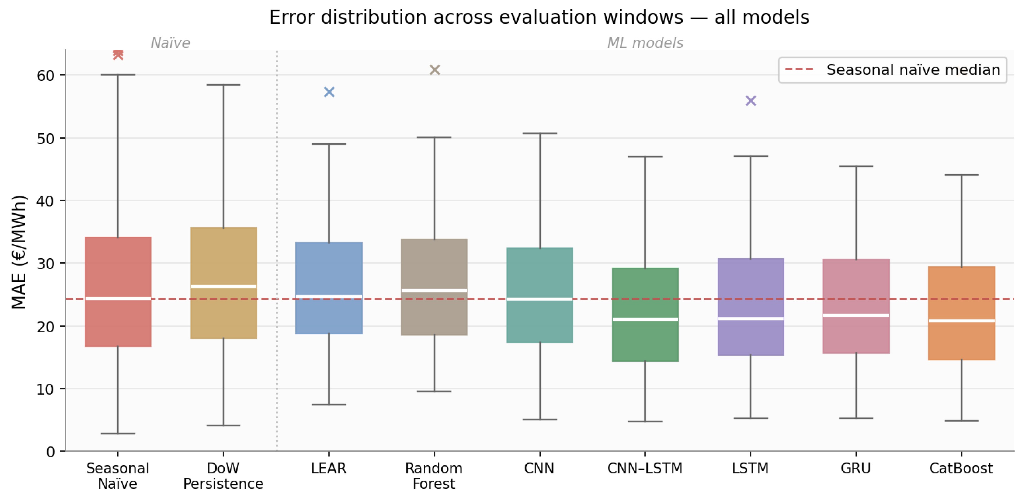
Figure 5 presents the distribution of weekly MAE across all 50 weekly rolling forecast windows for every model considered, including the two naïve baselines and the LEAR statistical reference; this stage serves as an initial screen on a common endogenous feature set (the feature groups active at each stage are mapped in Table 5). The corresponding summary statistics are reported in Table 7. The two front-runners are CatBoost-recursive (MAE 22.93 €/MWh, RMSE 31.04, ${\mathrm{MASE}}_{168}$ 0.889) and CNN–LSTM (22.91, 31.15, 0.894); their mean-MAE gap is negligible (0.02 €/MWh) and, as the significance tests below confirm, not statistically distinguishable. Both clearly lead the remaining candidates: LSTM and GRU follow (23.3–23.4 €/MWh), then CNN (25.2), while Random Forest (27.3) and LEAR (27.2) fall just behind the seasonal-naïve baseline (26.1) at this week-ahead horizon. Only the five strongest learners attain ${\mathrm{MASE}}_{168}<1$ (i.e., beat the in-sample seasonal naïve); LEAR’s degradation is consistent with the difficulty a purely linear autoregressive model faces in extrapolating 168 h ahead, in contrast to its strong day-ahead performance reported by Lago et al. [3]. Training cost is comparable across the neural models and CatBoost (21–33 s per monthly recalibration), with Random Forest the clear outlier (113 s, and ∼14 s per forecast against <0.4 s for the others). We carry the two front-runners—together with a direct multi-horizon CatBoost variant—into a focused, significance-tested comparison over the full 2024 year (Section 7.2). The endogenous (NW) configuration used as the AOI reference baseline in Section 7.6 settles at a closely comparable 23.2 €/MWh.

The two leading learners reduce mean MAE by about 12% relative to the seasonal-naïve baseline (26.1 €/MWh) and reach ${\mathrm{MASE}}_{168}\approx 0.89$. The margin over the naïve baseline is smaller than is sometimes seen at the day-ahead horizon, reflecting the strength of weekly seasonality as a week-ahead predictor: the seasonal naïve is competitive at the median but has a heavier right tail on volatile weeks, which the learners smooth. Notably, LEAR—a very strong day-ahead benchmark [3]—does not transfer to this 168-hour-ahead setting, finishing below even the naïve baselines (${\mathrm{MASE}}_{168}=1.05$); a purely linear autoregression struggles to project the full weekly trajectory, which motivates the non-linear models.

CatBoost-recursive and CNN–LSTM are separated by only 0.02 €/MWh in mean MAE, with CatBoost marginally ahead on RMSE and MASE and CNN–LSTM marginally ahead on MAE; their weekly-MAE distributions overlap almost entirely (Figure 5). The choice between them therefore cannot be made on the screen alone and is resolved by the significance-tested comparison of the next subsection.

7.2. Focused Comparison and Significance Testing

To put the screening result on a firmer footing, the full benchmark was re-evaluated on weekly rolling origins spanning the whole of 2024. To leave no ambiguity about the design: the evaluation period is the 2024 out-of-sample year (with 2025 held out entirely); each origin issues a 168-h recursive forecast; the start day of the week is rotated across origins so the result does not depend on a fixed weekday; and every origin is trained on an expanding window of strictly preceding data that begins in 2023 and ends just before it. The window is anchored at a fixed 2023 start and grown to each origin rather than rolled forward at fixed length; because all models share the same window at each origin, the differences reported below reflect the models, not their training data. Pairwise accuracy is assessed with the Diebold–Mariano (DM) test [64], using the Harvey–Leybourne–Newbold small-sample correction [65] and a Newey–West long-run variance, applied to the per-origin MAE differential.

Table 8. Diebold–Mariano tests of CatBoost-recursive against every benchmark on the no-weather (endogenous) scenario, per-origin MAE differential over weekly origins in 2024. The differential is $\overline{\Delta }={\overline{\mathrm{MAE}}}_{\mathrm{CatBoost}-\mathrm{rec}}-{\overline{\mathrm{MAE}}}_{\mathrm{B}}$; a negative value favours CatBoost-recursive. The two front-runners, CNN–LSTM and a direct multi-horizon CatBoost, are examined further across weather scenarios in Table 9.

CatBoost-Recursive vs. B	$\overline{\mathbf{\Delta }}$ (€/MWh)	p-Value
Seasonal Naïve	$-3.18$	$0.12$
DoW Persistence	$-3.79$	$0.004$
LEAR	$-4.24$	$6.0\times {10}^{-3}$
Random Forest	$-4.37$	$0.006$
CNN	$-2.25$	$0.15$
LSTM	$-0.40$	$0.79$
GRU	$-0.51$	$0.71$
CNN–LSTM	$+0.02$	$0.99$

reports the test of the selected model, CatBoost-recursive, against every other candidate on the endogenous (no-weather) configuration, which is the cleanest like-for-like comparison because all learners then share an identical feature set.

Each reported p-value is the probability of observing a per-origin MAE differential at least as large as the one measured if the two models were in fact equally accurate; a value below the conventional $0.05$ threshold therefore signals a statistically significant difference, while a larger value means the observed gap is within week-to-week sampling noise. On endogenous features, CatBoost-recursive significantly outperforms the LEAR benchmark, the day-of-week persistence baseline, and Random Forest ($p=0.006$, $0.004$, $0.006$). Its advantage over the seasonal-naïve baseline and the plain CNN, although sizeable in mean MAE (3.2 and 2.3 €/MWh), is not statistically significant at the per-origin level ($p=0.12$ and $0.15$): with only a single year of weekly origins, the week-to-week variance of MAE is large, which limits the power of the test at this week-ahead horizon and is consistent with the heavy right tail of the seasonal naïve on volatile weeks noted above. CatBoost-recursive is statistically indistinguishable from the three recurrent architectures LSTM, GRU, and CNN–LSTM ($p=0.79$, $0.71$, $0.99$). Of all eight competitors the hybrid CNN–LSTM is the closest match: its mean-MAE differential is essentially zero ($+0.02$ €/MWh) and its p-value of $0.99$ is the highest in the table, so it is statistically the least distinguishable from CatBoost-recursive. No model significantly beats CatBoost-recursive, and CNN–LSTM matches but does not exceed it. Because CNN–LSTM is the only model that genuinely rivals the selected one, it is the natural focus of the deeper, scenario-by-scenario comparison that follows.

This leaves two genuine contenders, which we examine head-to-head across all three weather scenarios: the hybrid CNN–LSTM (the joint front-runner on the screen) and a direct multi-horizon CatBoost (which predicts each day’s 24 prices jointly with a multi-output model, day-block by day-block, rather than rolling a one-step model forward).

Table 9. Head-to-head Diebold–Mariano tests against the selected CatBoost-recursive model across weather scenarios (per-origin MAE differential, the weekly origins of 2024). The differential is $\overline{\Delta }={\overline{\mathrm{MAE}}}_{\mathrm{CatBoost}-\mathrm{rec}}-{\overline{\mathrm{MAE}}}_{\mathrm{B}}$; a negative value favours CatBoost-recursive. The no-weather CatBoost-recursive vs. CNN–LSTM comparison is a tie in Table 8 ($p=0.99$); this focused run uses an earlier CNN–LSTM checkpoint (no-weather MAE 23.3 against 22.9 in the screen), which does not affect the rankings.

Vs. B	Scenario	$\overline{\mathbf{\Delta }}$ (€/MWh)	p-Value
CatBoost-direct	No weather	$-6.44$	$7.3\times {10}^{-5}$
	TMY	$-4.79$	$2.6\times {10}^{-3}$
	Forecasted weather	$-4.61$	$8.2\times {10}^{-5}$
CNN–LSTM	TMY	$-0.40$	$0.83$
	Forecasted weather	$-3.27$	$2.8\times {10}^{-3}$

reports the pairwise tests.

Two clear conclusions emerge. First, the recursive roll-out is the right construction: CatBoost-recursive beats the direct multi-horizon variant by a wide and significant margin in every scenario (no-weather $-6.44$, TMY $-4.79$, forecasted-weather $-4.61$ €/MWh; $p\le 2.6\times {10}^{-3}$ throughout). Second, CatBoost-recursive and CNN–LSTM are statistically tied on endogenous and climatological inputs (no-weather $p=0.99$, Table 8; TMY $p=0.83$) but the tie breaks once an operational weather forecast is supplied, where CatBoost-recursive becomes significantly more accurate (forecasted weather, $\overline{\Delta }=-3.27$ €/MWh, $p=2.8\times {10}^{-3}$): the gradient-boosting model extracts more value from the weather signal than the hybrid network does.

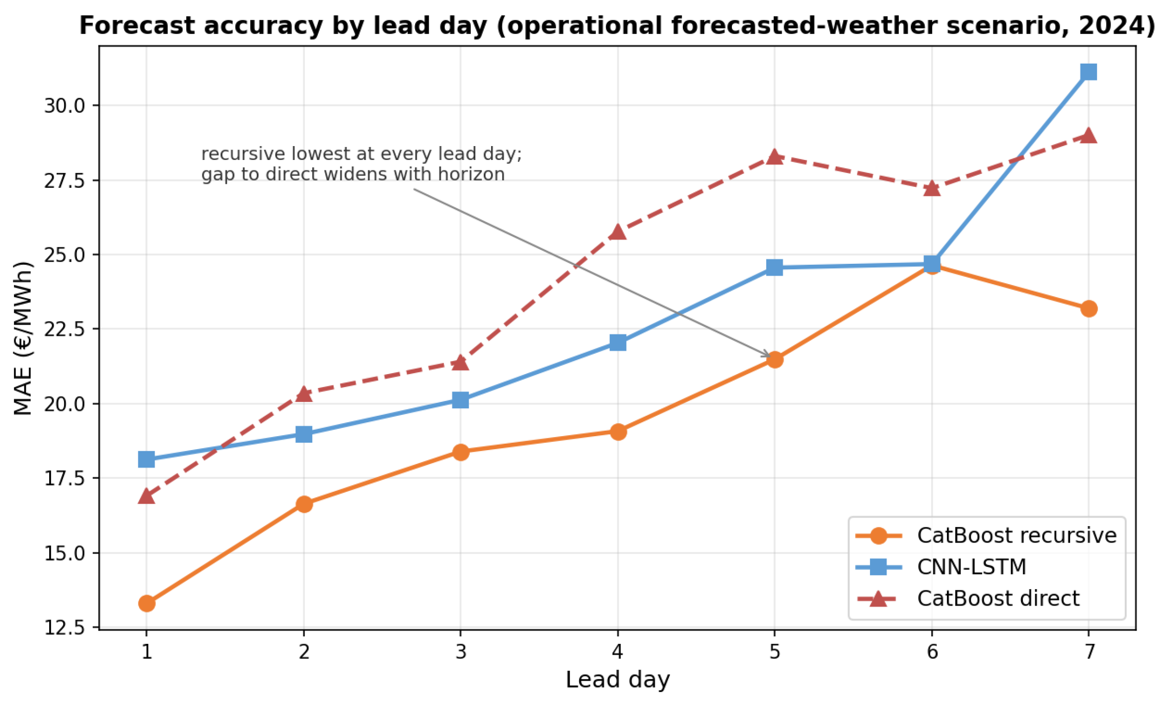
CatBoost-recursive has the lowest error at all seven lead days—including day 1, where no recursion error has yet accumulated (13.3 versus 16.9 €/MWh for the direct variant and 18.1 for CNN–LSTM)—and its margin over the direct construction broadens as the horizon lengthens. CNN–LSTM tracks CatBoost-recursive closely over the first few days but deteriorates faster at the weekly tail.

Figure 6 reports the corresponding lead-day MAE profile under the operational forecasted-weather scenario.

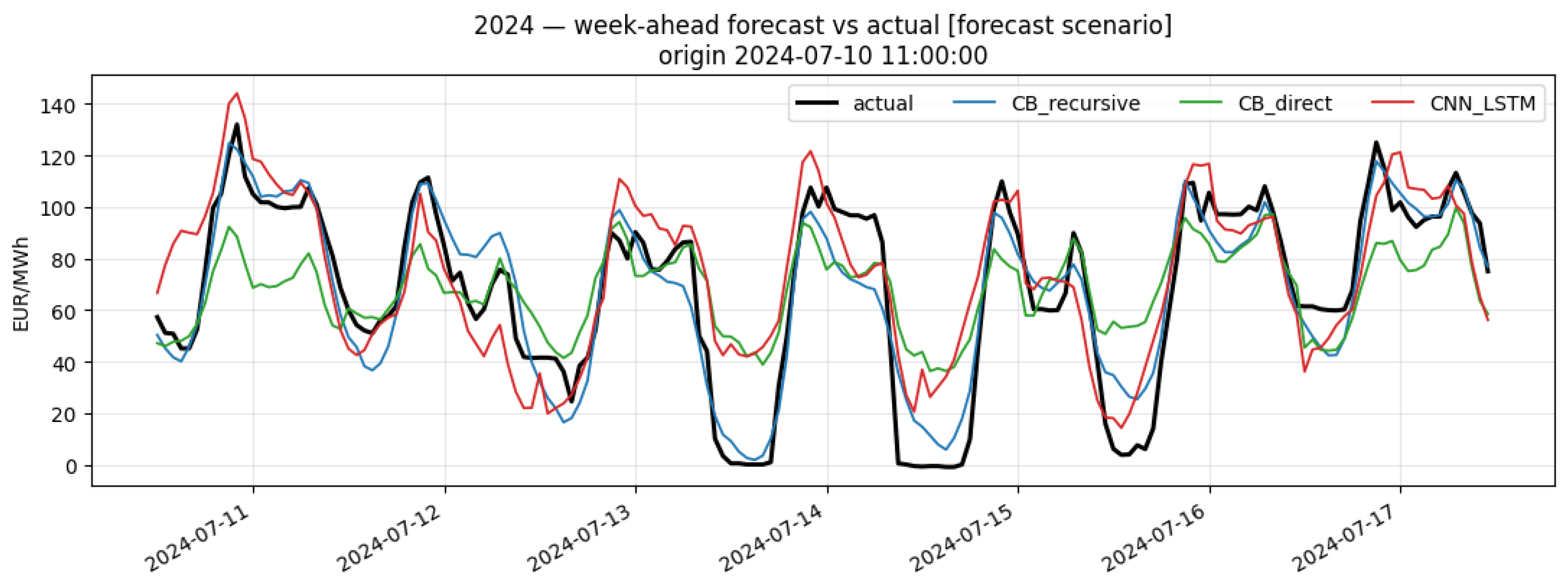
This pattern is visible at the level of an individual week. Figure 7 overlays the three contenders against the realised price for a representative origin (10 July 2024) under the forecasted-weather scenario: CatBoost-recursive and CNN–LSTM both reproduce the daily peak/trough structure and the weekly envelope, whereas the direct multi-horizon CatBoost flattens the extremes—it underestimates the evening peaks and overestimates the overnight troughs—which is precisely the behaviour that accumulates into its larger lead-day and aggregate errors.

Adding forecasted weather lowers CatBoost-recursive to 19.53 €/MWh, and it remains the best model in every feature scenario: against the direct multi-horizon variant the gap is $-4.61$ €/MWh and against CNN–LSTM $-3.27$ €/MWh under forecasted weather (Table 9).

This ranking is confirmed on the fully out-of-sample 2025 year (used for nothing during development): with forecasted weather, CatBoost-recursive attains MAE 21.39 €/MWh (${\mathrm{MASE}}_{168}=0.70$) whereas CNN–LSTM rises to 26.11 €/MWh, a gap that remains significant (DM $p=1.6\times {10}^{-4}$). The tree-based recursive model thus generalises to the held-out year more reliably than the hybrid network. Training cost is comparable to the neural models (Table 7), so the selection rests not on speed but on accuracy once weather is included, robustness to the held-out year, and a simpler, more stable training procedure—a single gradient-boosting model rather than a neural architecture requiring per-sample normalisation and early-stopping tuning. CatBoost-recursive is therefore selected for all subsequent analyses.

7.3. Forecast Error Evolution and Regime-Stratified Performance

To place the 2024 benchmark within a wider historical context, the same fixed CatBoost configuration was applied retrospectively to each year from 2019 to 2024. For each target year X, the model was trained only on data from the beginning of year $X-1$ up to the forecast origin. This keeps the training-window length broadly comparable across years, so that differences in

Table 10. Regime-stratified price and forecast-error statistics (CatBoost, NW). Volatility: 30-day rolling standard deviation of the daily price (€/MWh), regime average.

Regime	Mean Price (€/MWh)	Price Volatility (€/MWh)	MAE (€/MWh)	RMSE (€/MWh)
Pre-crisis (2020–mid-2021)	45.3	21.0	6.8	9.1
Gas crisis (mid-2021–2022)	167.5	69.3	32	37.4
Post-crisis (2023–2024)	75.0	45.4	23.2	26.9

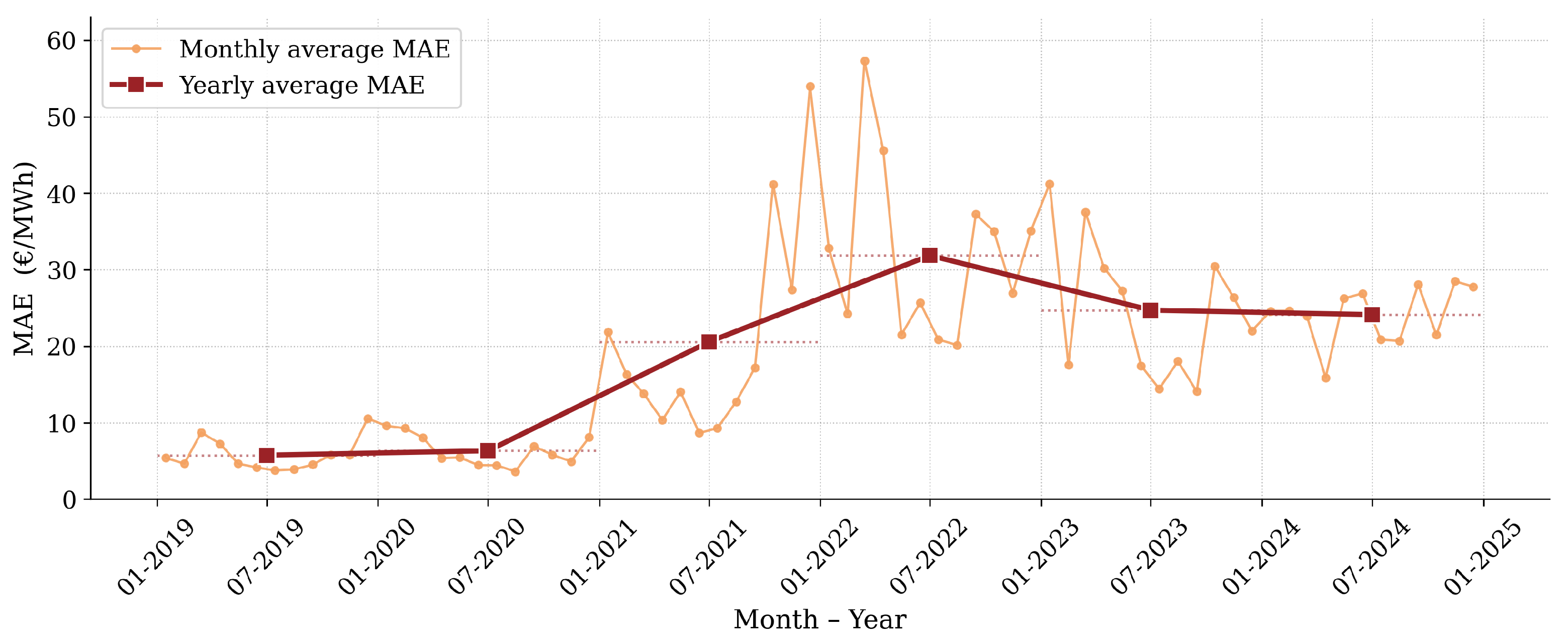
mainly reflect changing market conditions rather than a mechanically expanding training sample. This pass is illustrative context for how forecast difficulty co-moved with the crisis and is distinct from the rigorous model comparison of Section 7.2. The resulting monthly and annual average MAEs are displayed in Figure 8.

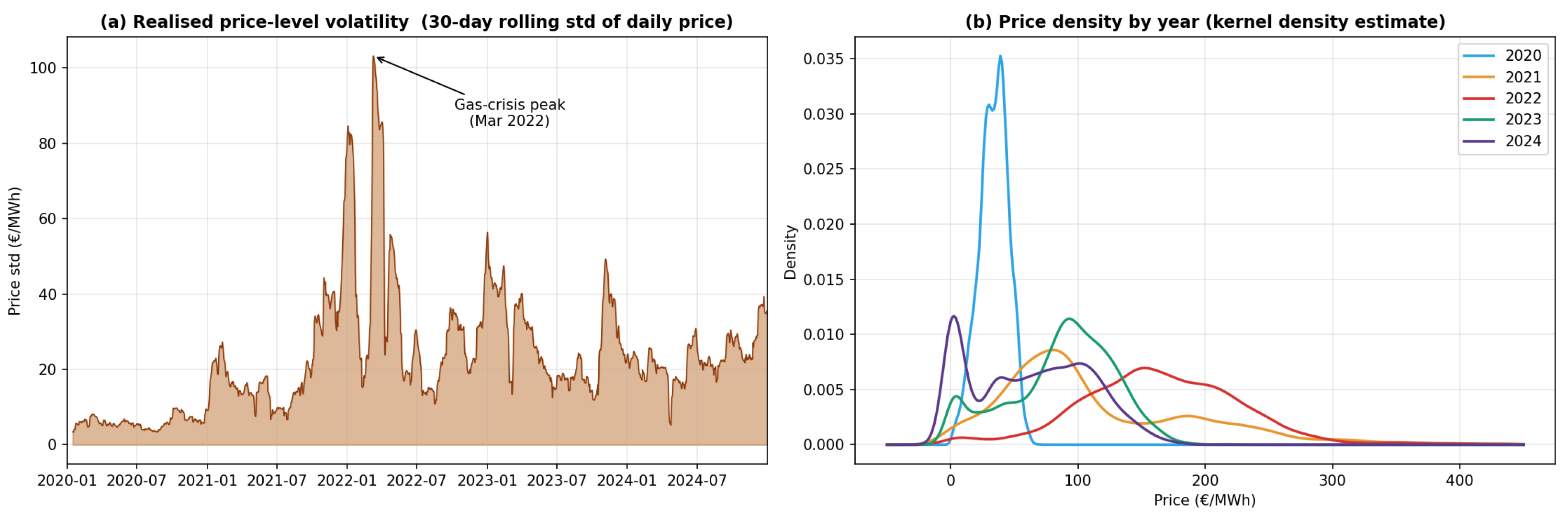
The picture that emerges is one of pronounced regime dependence. Annual MAEs of 6–7 €/MWh in 2019–2020 rose sharply to 22 and 32 €/MWh in 2021 and 2022 respectively, before settling at around 23 €/MWh by the end of 2024 as the market normalised. The corresponding regime-level statistics are summarised in Table 10. During the crisis period from mid-2021 to end-2022, both the price level and the realised volatility rose by approximately an order of magnitude, and the CatBoost week-ahead MAE moved from roughly 7 to about 26 €/MWh. The relationship is consistent with a component of forecast difficulty that scales with market volatility (R² = 0.30 between monthly price-level volatility and monthly MAE in 2024), and suggests that part of the error observed during this period reflects inherent price unpredictability rather than model inadequacy alone. The subsequent post-crisis normalisation in 2023–2024 brought forecast errors back to a level close to, though still somewhat above, the pre-crisis baseline. Several factors could plausibly contribute to this residual gap—including more frequent negative-price episodes, changing gas-price dynamics, higher renewable penetration, and evolving bidding behaviour—but the present feature set does not include cross-border flow variables and therefore cannot isolate the role of interconnection; we accordingly treat these as candidate explanations rather than established effects. Interconnection in particular cannot be exploited at this horizon in any case: realised cross-border flows are published only after the day-ahead auction, and the forecasted transfer capacity available beforehand is only weakly correlated with price (Section 9).

7.4. Training Period Sensitivity

Table 11. Forecasting error differences versus 2023-baseline training period.

Training Year	$\mathbf{\Delta }$ MAE	$\mathbf{\Delta }$ RMSE
2023 (baseline)	$0\%$	$0\%$
2022	$+12.85\%$	$+10.66\%$
2021	$+7.11\%$	$+6.32\%$

shows that, among the three single-year training windows tested, the model trained on 2023 data yields the best 2024 performance. Training on 2022 crisis data instead degrades MAE by 12.85%, while training on 2021 data adds 7.11%. Within this single-year comparison, the immediately preceding year is therefore the most informative starting point, which motivates anchoring the deployed expanding window at 2023 rather than reaching back into the crisis years. Multi-year rolling strategies with alternative start years were not exhaustively explored and could in principle yield different results.

The configurations exercised in the analyses that follow are exactly those mapped in Table 5. The common operational benchmark and the weather-scenario experiments rely exclusively on features available at the time of forecast issuance, so that they correspond to genuinely deployable settings; the full-feature configuration used for the importance analysis additionally incorporates historical weather (HW) and realised energy-system variables, and is therefore best understood as an ex-post explanatory upper bound rather than an operational forecast.

7.5. Categorical Feature Importance

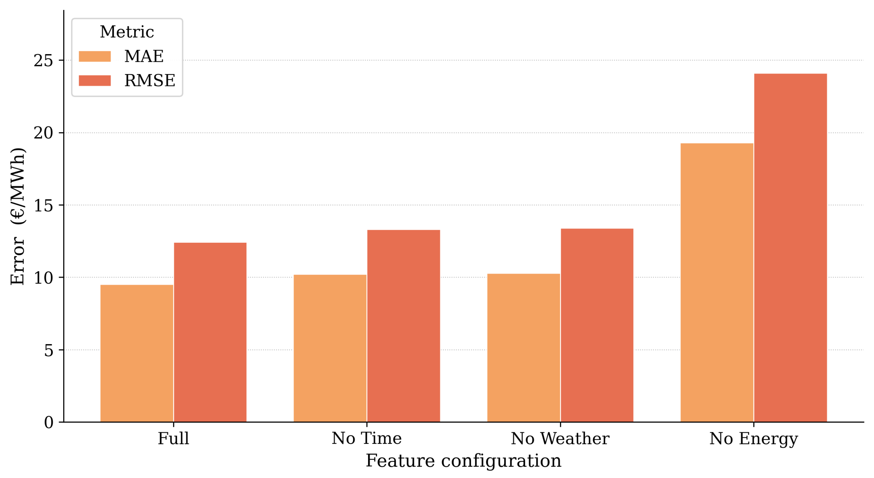
The leave-one-out experiment presented in this subsection differs in scope from the weather-scenario comparison reported in Section 7.7, and the distinction is important to bear in mind when interpreting the results. The baseline of the present experiment is the full feature set (time, weather, and energy variables), and each feature category is then removed in turn from this baseline. As a consequence, the “No Weather” configuration shown in Figure 9, which yields an MAE of approximately 11 €/MWh, retains the energy features and is therefore not directly comparable with the no-weather row in the weather-scenario analysis reported later, where both weather and energy features are absent and the MAE rises to about 23 €/MWh. For this reason, the analysis that follows should be read as an ex-post explanatory upper bound rather than as a fully operational week-ahead forecast, since the energy features incorporate realised system conditions that would not be available to a forecaster at the time of issuance.

With this caveat in mind, the experiment yields a clear ranking. Removing the energy features alone causes the MAE to roughly double, from 9.52 to 20.4 €/MWh, an effect substantially larger than that observed when either the time or the weather features are removed. This finding provides empirical support for the theoretical argument developed in Section 2, in which the instantaneous generation mix, and in particular the level of natural-gas-fired generation, was identified as a direct observable proxy for the position of the market-clearing price on the merit-order stack. The doubling of MAE upon removal of the energy block is consistent with this interpretation: when the model loses sight of the dispatch state, it can no longer locate the clearing price along the supply curve, and forecast accuracy degrades accordingly.

7.6. Feature Importance: AOI and LOO

This analysis is deliberately exploratory: rather than asking what causes the price, it asks which contemporaneous system variables, if their realised values were known, would most reduce week-ahead error—thereby revealing where forecast skill is gained or lost and which fundamentals are worth forecasting explicitly. Because these variables are strongly correlated with one another (gas-fired generation, for instance, moves together with demand, renewable output, imports, and fuel prices), no single number captures a feature group’s “importance”; we therefore probe each group in two complementary ways—once on its own and once in the presence of all the others—and read the two together.

We use two complementary measures of predictive importance. Add-one-in (AOI) importance is the accuracy gain from adding a single feature group j to the endogenous baseline (price lags and calendar), i.e., how much that group helps on its own; leave-one-out (LOO) importance is the accuracy loss from removing group j from the full-information model, i.e., its marginal contribution given everything else. The two need not agree: under correlated predictors a group can be informative in isolation (high AOI) yet redundant at the margin (low LOO), or vice versa. We emphasise that “LOO” here denotes leave-one-feature-out importance and is unrelated to leave-one-out cross-validation. Formally,

$$I_{\mathrm{AOI},j}={\mathrm{MAE}}_{\mathrm{base},\mathrm{AOI}}-\mathrm{MAE}\left(f_j\right),{\mathrm{MAE}}_{\mathrm{base},\mathrm{AOI}}=23.2€/\mathrm{MWh};$$

$$I_{\mathrm{LOO},j}=\mathrm{MAE}(F\setminus \left\{f_j\right\})-{\mathrm{MAE}}_{\mathrm{full}},{\mathrm{MAE}}_{\mathrm{full}}=9.5€/\mathrm{MWh}.$$

The two reference points bound the reducible error: the operational endogenous baseline reaches 23.2 €/MWh, whereas a model with the full set of realised system variables (an ex-post upper bound, not an operational configuration) reaches 9.5 €/MWh. The difference, $23.2-9.5=13.7$ €/MWh, is therefore the error that perfect knowledge of contemporaneous system state would close, of which natural-gas generation is the single largest contributor.

It is important to interpret these quantities correctly. They measure predictive informativeness, not causation: gas-fired generation is highly informative because it proxies the position of the marginal unit in the merit order, but it is itself correlated with demand, renewable output, imports, and fuel prices, so the analysis does not isolate a causal effect of gas generation on price. We therefore present gas generation as the dominant predictive and explanatory feature, consistent with the marginal-pricing mechanism, while refraining from causal attribution. The AOI/LOO ranking is likewise an ordering of informativeness rather than a precise, confidence-bounded ranking; quantifying its robustness (e.g., by bootstrap or across sub-periods) is left to future work.

Negative AOI importance (Water Reservoir: $-0.05$; Total Load: $-0.66$) indicates that these features marginally worsen accuracy when used in isolation. Their signal is already encoded in the lagged price history; they add noise when used alone but contribute marginally within the full context (positive LOO importance).

Table 12. AOI and LOO feature importance (MAE). Base AOI = 23.2 (NW baseline); full-model LOO = 9.52. Negative AOI: feature degrades accuracy when used alone.

Feature	AOI MAE	LOO MAE	Imp. AOI	Imp. LOO
Natural Gas	12.65	11.22	10.55	1.70
Hydro Cons.	13.43	10.78	9.77	1.26
Wind Onshore	17.44	9.96	5.76	0.44
Wind Speed	19.18	9.57	4.02	0.05
Hydro Storage	20.25	9.70	2.95	0.18
Wind Dir	20.47	9.51	2.73	−0.01
Oil	20.77	10.24	2.43	0.72
Biomass	20.84	9.72	2.36	0.20
Gas Price	21.06	9.77	2.14	0.25
Waste	21.45	9.68	1.75	0.16
Other Renew.	21.45	9.19	1.75	−0.33
Hard Coal	21.46	9.81	1.74	0.29
Radiation	21.47	9.63	1.73	0.11
Nuclear	21.72	9.59	1.48	0.07
Other	21.72	9.72	1.48	0.20
Precip	21.72	9.64	1.48	0.12
Humidity	21.78	9.57	1.42	0.05
Run-of-river	21.81	10.43	1.39	0.91
Temp	21.93	9.57	1.27	0.05
Dew Point	22.05	9.56	1.15	0.04
Solar	22.90	9.11	0.30	−0.41
Water Reservoir	23.25	9.74	−0.05	0.22
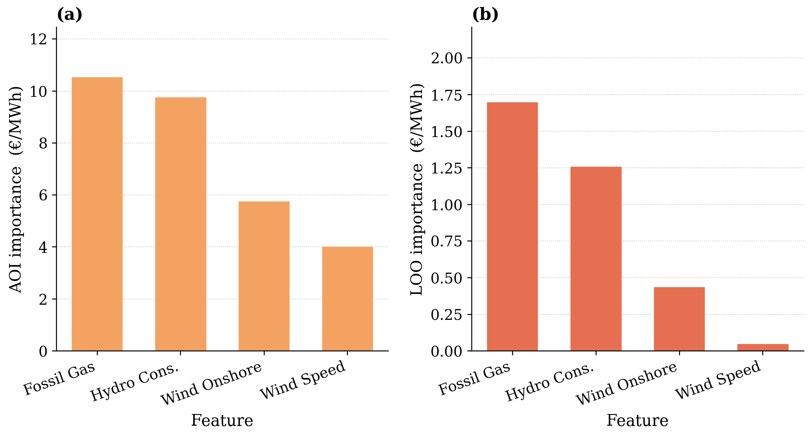
Total Load	23.86	9.66	−0.66	0.14

and Figure 10 present the full results. Natural gas and pumped-hydro consumption are the dominant features, directly consistent with the merit-order argument: both reflect the instantaneous balance between supply and demand at the margin. Wind Onshore ranks third, as large wind surpluses push gas turbines off the margin, suppressing or inverting the clearing price [13].

The top four features combined (Natural Gas, Hydro Cons., Wind Onshore, Wind Speed) achieve MAE ≈ 10.6, only ∼1.1 €/MWh above the full model’s 9.52.

7.7. Weather Input Scenarios

The experiment reported in this subsection isolates the contribution of weather information to forecast accuracy, and for this reason the model is trained on time, lagged-price, and weather features only, with no energy variables included. This design choice is what distinguishes the present analysis from the categorical leave-one-out experiment of Section 7.5: the NW row in

Table 13. Forecast error by weather-input scenario, averaged over 366 daily-issued 168 h origins in 2024 (every calendar day). All runs use time, lags, and weather only; energy features are excluded. The with-weather scenarios share one model trained on actual weather and differ only in the weather supplied at inference.

Scenario	MAE	RMSE
Actual weather (HW, oracle upper bound)	19.31	25.42
Forecasted weather (FW, operational)	20.02	26.49
TMY climatology	23.48	31.82
No weather (NW)	23.73	31.59

, with an MAE of 23.7 €/MWh, corresponds to a configuration in which neither weather nor energy features are available, whereas the “No Weather” bar in Figure 9, with an MAE of approximately 11 €/MWh, retains the energy block and therefore reflects a much narrower deprivation of information.

This table represents averages on a 168-h forecasted window rolling every day of 2024 (365 windows) in a way to give the most realistic averages. Three observations now follow. First, the operational forecast (FW) is the best weather input: it sits only 0.71 €/MWh above the perfect-foresight oracle (HW) and recovers about 84% of the oracle’s improvement over the no-weather baseline, so the day-ahead numerical weather prediction (NWP) product is skilful enough to capture most of the realisable weather value. Second, TMY climatology is essentially tied with the no-weather baseline (23.48 vs. 23.73 €/MWh): a generic seasonal climatology adds little once price lags are present, because it carries no information about the specific weather of the forecast week. Third, the advantage of real weather information is strongly horizon-dependent, as shown by the per-lead-day decomposition in

Table 14. Weather-scenario MAE (€/MWh) by forecast lead-day, 366 daily origins in 2024.

Scenario	D1	D2	D3	D4	D5	D6	D7
Actual (HW)	13.58	18.48	19.75	20.57	20.69	20.87	21.23
Forecasted (FW)	14.35	18.78	20.02	20.96	21.20	22.01	22.84
TMY	14.63	21.29	23.72	25.11	26.10	26.65	26.86
No weather (NW)	14.50	21.15	23.64	25.52	26.73	27.32	27.26

: at Day 1 all scenarios are within 0.3 €/MWh (recent price lags dominate and the weather signal is redundant), whereas by Day 7 the forecast advantage over no-weather grows to about 4.4 €/MWh and the operational forecast tracks the oracle closely throughout. This horizon profile is exactly what one expects—weather matters where the autoregressive signal has decayed—and it explains why the value of weather data is easy to miss in horizon-pooled metrics.

These results invert the earlier interpretation: operational weather forecasts are not a liability but the recommended weather input for week-ahead EPF in MIBEL, and their benefit is concentrated at the multi-day horizons that motivate week-ahead forecasting in the first place. Consistent with this, recent evidence shows weather predictions improving electricity-price forecasts at longer horizons [66], and renewable-generation forecast errors propagating into imbalance volumes and spot prices [67,68].

7.8. Optimal Lag Selection and Horizon Performance

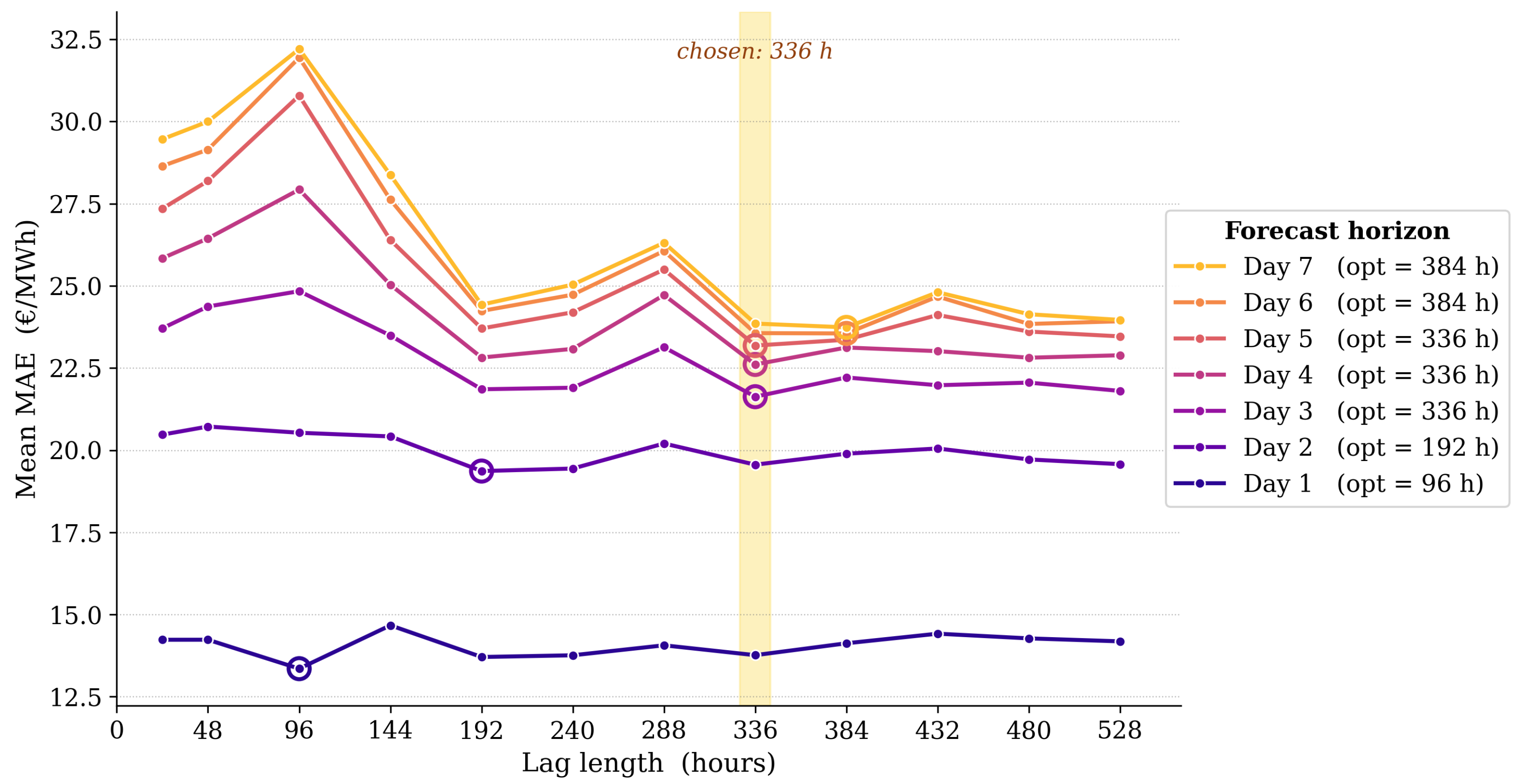
The optimal lag window is investigated through a sweep over lag lengths ranging from 48 to 384 h, performed separately for each forecast day from Day 1 to Day 7. The MAE as a function of lag length is shown in Figure 11, and the per-horizon optima are reported in

Table 15. Optimal lag window and corresponding MAE for each forecast day.

Forecast Day	Optimal Lag (h)	MAE (€/MWh)
Day 1	96	13.880
Day 2	192	17.035
Day 3	336	19.410
Day 4	336	20.861
Day 5	336	21.905
Day 6	384	22.612
Day 7	384	23.051

.

A clear pattern emerges from Table 15: the optimal lag window grows with the forecast horizon, increasing from 96 h for Day 1 to 384 h for Day 7. This behaviour is consistent with the autocorrelation analysis presented earlier, in which the autocorrelation function of the price series exhibits a strong peak at 168 h and retains substantial persistence up to 336 h. The predictive content of these long lags is therefore most valuable for multi-day-ahead steps, where short-term autocorrelation alone is no longer sufficient. For operational simplicity, a single lag window of 336 h is adopted across all forecast horizons. The cost of this uniform choice is modest: even in the worst case (Day 6 and Day 7, which would individually prefer 384 h), the MAE penalty relative to the per-horizon optimum does not exceed 0.7 €/MWh.

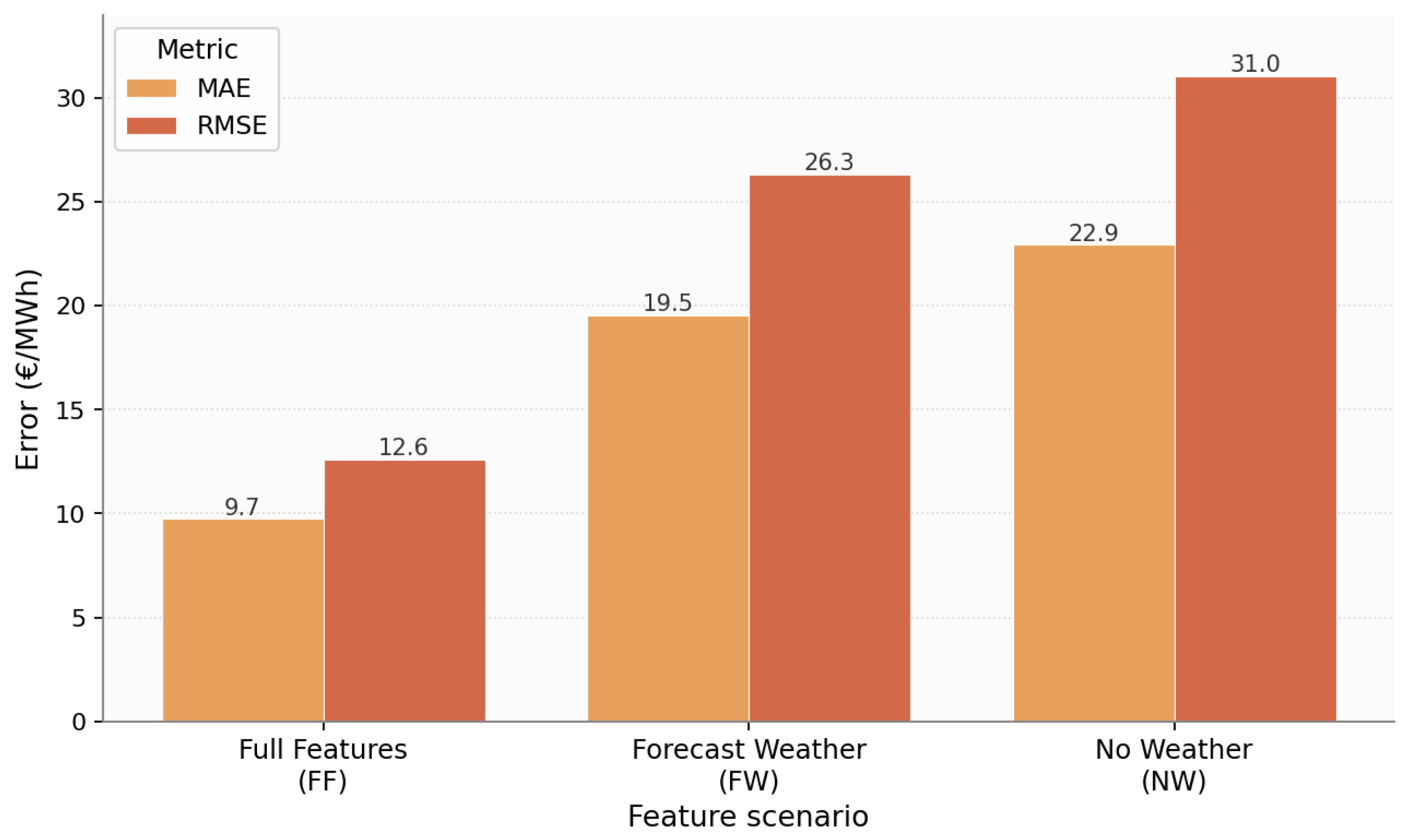
After re-tuning the model hyperparameters at the chosen 336-h lag window, the final error metrics are obtained as follows: the full-feature configuration (FF) yields an MAE of 9.74 €/MWh and an RMSE of 12.62 €/MWh; the operational forecasted-weather configuration (FW) yields 19.53 and 26.32 €/MWh respectively; and the no-weather baseline (NW) yields 22.93 and 31.04 €/MWh. The corresponding error profiles are displayed in Figure 12.

7.9. Monthly Error Trends (2024)

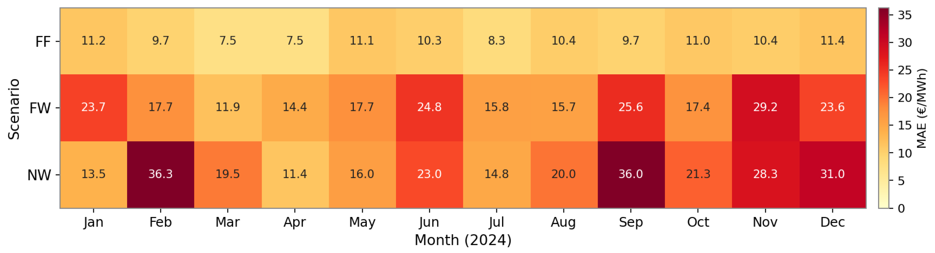
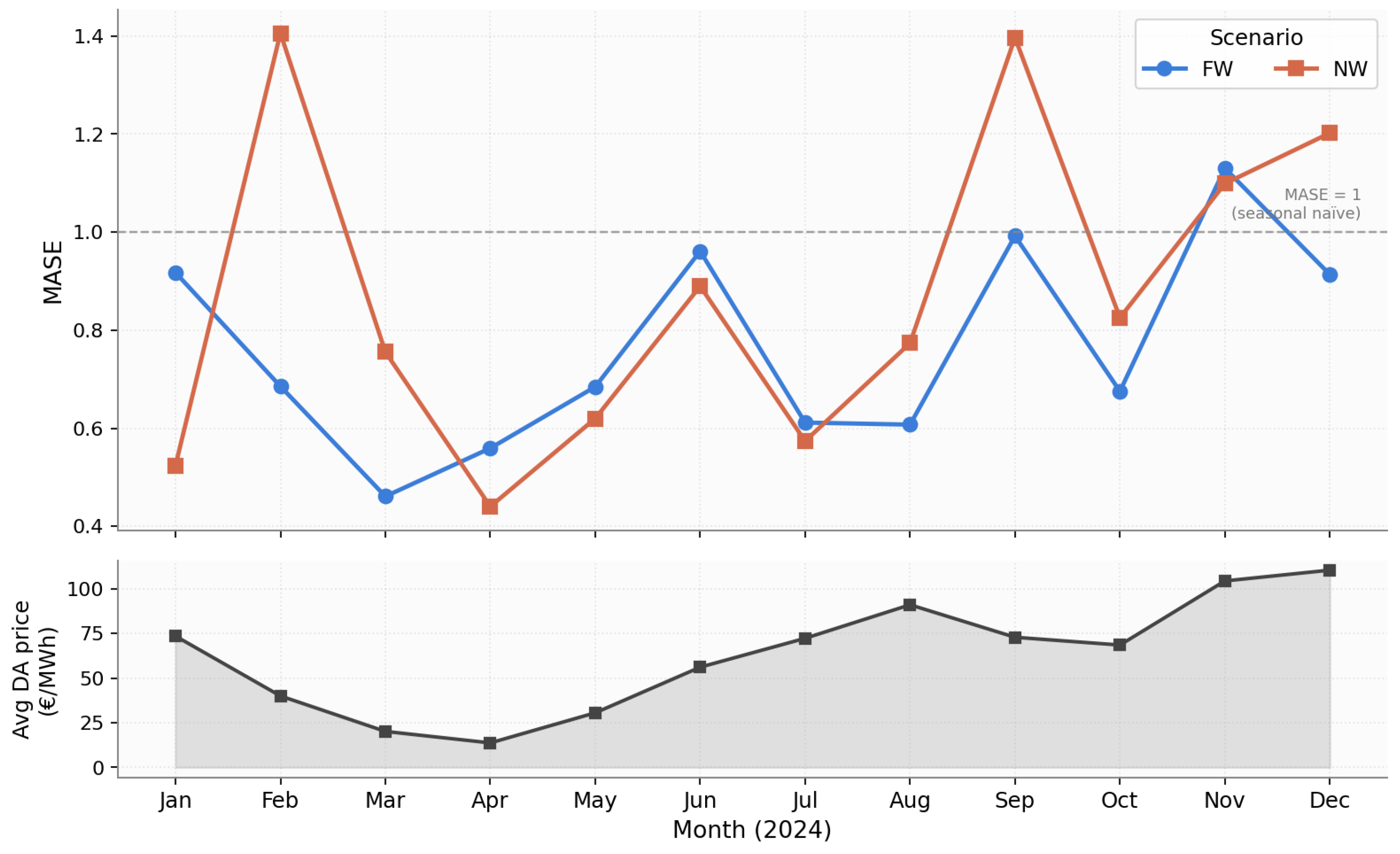
Figure 13 and Figure 14 resolve the scenarios month by month. The no-weather model (NW) is most error-prone in the volatile months, peaking in February and September (≈36 €/MWh) and breaching the in-sample seasonal-naïve benchmark there (MASE > 1); supplying an operational weather forecast (FW) lowers the error in almost every month and holds the MASE below 1 in all months but November. The ex-post full-feature scenario (FF), shown for reference in the heatmap, stays at 8–11 €/MWh in every month, so most of the residual monthly error in the deployable FW scenario reflects forecast uncertainty rather than irreducible noise. Both deployable scenarios track the price level—the scaled error is smallest in the low-priced spring months and largest in the high-priced, weather-driven winter—consistent with the marginal-cost pricing framework.

8. Battery Arbitrage Model and Results

A price-taking battery energy storage system is modelled [69,70,71,72] with power limit $P_{max}=200\mathrm{MW}$, energy capacity $E_{max}=800\mathrm{MWh}$ (a 4-h asset), and symmetric round-trip efficiency ${\eta }_{\mathrm{RT}}=0.90$. Charging and discharging efficiencies are therefore set as

$${\eta }_c={\eta }_d=\sqrt{{\eta }_{\mathrm{RT}}}\approx 0.9487.$$

(5)

The model uses an hourly time step throughout, so power and energy are linked directly over each optimisation interval. For each rolling optimisation window, three decision variables are defined for every hour $t=1,\dots ,T$ of the horizon: charging power $c_t\ge 0$ (MW; buy), discharging power $d_t\ge 0$ (MW; sell), and state of charge $s_t\in [0,E_{max}]$ (MWh). Dispatch is determined by the following linear programme:

$$\underset{c_t,d_t,s_t}{max}{\displaystyle \sum _{t=1}^T}{\widehat{p}}_t\left(d_t-c_t\right),$$

(6)

subject to

$$\begin{array}{cc}\hfill s_t& =s_{t-1}+{\eta }_c{c}_t-{\displaystyle \frac{1}{{\eta }_d}}{d}_t,\forall t=1,\dots ,T,\hfill \end{array}$$

(7)

$$\begin{array}{cc}\hfill 0& \le c_t\le P_{max},0\le d_t\le P_{max},\hfill \end{array}$$

(8)

$$\begin{array}{cc}\hfill 0& \le s_t\le E_{max}.\hfill \end{array}$$

(9)

Under this formulation, simultaneous charging and discharging is economically dominated because ${\eta }_c{\eta }_d<1$; accordingly, such behaviour does not arise in the optimal LP solutions considered here.

A natural question concerns the role of a terminal state-of-charge condition,

$$s_T=s_0,$$

(10)

which would force the battery to end each optimisation window at its initial charge. We do not impose Equation (10) in the reported results; instead we leave the terminal state free, so that the only difference between the two horizons below is the length of the look-ahead.

The dispatch schedule $\{c_t^{\star },d_t^{\star }\}$ is computed using the forecast price ${\widehat{p}}_t$ over the optimisation horizon. For the perfect-foresight (PF) benchmark, ${\widehat{p}}_t=p_t$, so realised prices replace forecasts and provide an upper-bound reference. In all other cases, the battery charges in hours forecast to be relatively cheap and discharges in hours forecast to be relatively expensive. After the optimisation is solved, only the first 24 h of the schedule are executed, and realised profit is settled against the observed market price $p_t$:

$${\pi }_{\mathrm{day}}={\displaystyle \sum _{t=1}^{24}}{p}_t\left(d_t^{\star }-c_t^{\star }\right).$$

(11)

Hence, the forecast determines the timing and magnitude of scheduled trades, whereas realised prices determine their monetary outcome. Forecast error therefore enters performance through mis-timed and mis-sized trades rather than through the settlement rule itself.

Both strategies are run as a receding-horizon controller that commits only the first 24 h and rolls forward one day at a time, carrying the realised end-of-day state of charge $s_{24}^{\star }$ as the next initial condition $s_0$. They differ solely in how far they look ahead when optimising: the 168 h strategy solves over the full 7-day forecast window ($T=168$) before committing 24 h, whereas the 24 h strategy sees only the day-ahead 24-h slice ($T=24$). The 24 h strategy therefore has no information beyond the current day and, lacking any reason to hold energy overnight, empties the battery at the end of every day; the 168 h strategy can instead retain energy across day boundaries when a more profitable opportunity is forecast later in the week. This isolates the value of the look-ahead, not of any terminal constraint. Annual profit is accumulated only over the 24-h execution layer, avoiding double counting across overlapping windows. Forecast value is then summarised using the value-capture ratio (VCR) and economic regret:

$$\mathrm{VCR}={\displaystyle \frac{{\Pi }_{\mathrm{model}}}{{\Pi }_{\mathrm{PF}}}},\mathcal{R}={\Pi }_{\mathrm{PF}}-{\Pi }_{\mathrm{model}},$$

(12)

where $\Pi$ denotes total annual realised profit. A VCR of unity indicates perfect value capture relative to PF, while economic regret measures the absolute opportunity cost associated with imperfect forecasts.

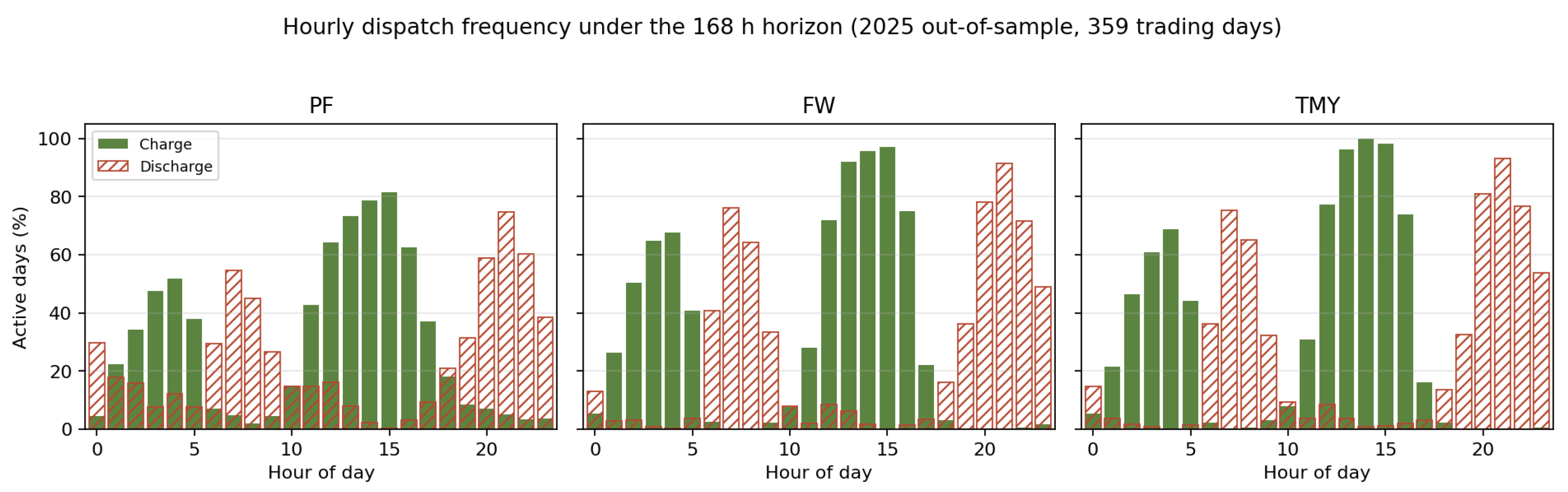
Before turning to the aggregate performance figures, it is instructive to examine the dispatch behaviour induced by each forecast. Figure 15 shows the fraction of trading days on which each hour-of-day contains active charging or discharging under the 168 h strategy. Across all models, discharging exhibits a clear bimodal structure, with a morning peak around 08:00–10:00 and an evening peak around 20:00–23:00, consistent with the main daily demand ramps. Charging is concentrated primarily in the overnight off-peak period (03:00–06:00), with a secondary cluster during the midday to afternoon trough (approximately 14:00–16:00), when prices are often depressed by solar generation. PF displays the sharpest and most concentrated charge–discharge pattern, reflecting the strongest temporal discrimination in the underlying price signal. TMY, by contrast, shows the broadest charging window and a smoother dispatch profile, consistent with a coarser forecast that provides less precise temporal guidance. FW lies between these extremes, most closely reproducing the PF dispatch structure.

The reference asset is parameterised on ENGIE’s Tarifa standalone battery in Andalusia—200 MW/800 MWh (a 4-h duration), the largest standalone BESS currently under development in Spain (its sister project Álora is 78 MW/312 MWh, also 4 h) [73]. The backtest is run on the fully out-of-sample 2025 year, providing a genuine forward test of forecast-driven dispatch. The dispatch model deliberately abstracts from several real-world costs in order to isolate the contribution of forecast quality. Battery degradation, cycling costs, variable O&M, transaction and imbalance charges, and market-impact effects are not modelled, and the price-taker assumption is maintained throughout. These simplifications mean that the reported profit figures represent an upper bound on achievable economic value under the tested forecasting configurations, rather than financial projections for a specific asset. Finally, because the price-taker LP is positively homogeneous of degree one in the rating, both profit (linearly) and the VCR (exactly) are determined by the energy-to-power ratio alone, so the value-capture ratios reported below are independent of the MW rating and transfer unchanged to any 4-h asset, including the smaller operational 3 MW/9 MWh Campo Arañuelo III unit in Cáceres [74].

Table 16. Annual battery-arbitrage results for the 4-h reference asset (200 MW/800 MWh, ${\eta }_{\mathrm{RT}}=0.90$) on the fully out-of-sample 2025 year, by price input and optimisation horizon. Profit $\Pi$ is in M€/yr; VCR is value capture relative to the perfect-foresight (PF) 168 h benchmark; $\Delta$ is the 24 h→168 h profit change. All reported percentages are independent of the MW rating.

Input	${\mathbf{\Pi }}_{24}$ (M€)	${\mathbf{\Pi }}_{168}$ (M€)	${\mathrm{VCR}}_{24}$ (%)	${\mathrm{VCR}}_{168}$ (%)	$\mathbf{\Delta }$ (%)
PF	19.19	20.05	95.6	100.0	4.5
FW	17.45	17.87	87.0	89.1	2.4
TMY	17.44	17.77	86.9	88.6	1.9

reports the arbitrage performance of the PF, FW, and TMY price inputs on the 2025 out-of-sample year. The dominant message is that the operational forecast captures most of the attainable value already at the 24 h horizon: under forecasted weather the VCR reaches 87% at 24 h and rises to 89% at 168 h, against a perfect-foresight ceiling of about 20.1 M€/yr for this 200 MW asset. The FW and TMY inputs yield very similar economic value (within one percentage point of VCR), even though FW has a substantially lower price MAE (Section 7.7). This is expected: arbitrage value depends on correctly ranking cheap and expensive hours rather than on the precise price level, so a coarser weather input can still drive near-optimal dispatch. The dispatch timing underlying these figures is shown in Figure 15: all three inputs charge predominantly in the overnight and midday-solar troughs and discharge into the morning and evening peaks, with PF producing the sharpest pattern, TMY the broadest, and FW closely tracking PF.

At this 4-h duration the benefit of extending the optimisation horizon from 24 h to 168 h is real but modest: the forecasted-weather gain is $+2.4\%$ (TMY $+1.9\%$), and even under perfect foresight the headroom is only $+4.5\%$. The 24 h-to-168 h gain can in principle arise from three distinct effects—terminal-state distortions, the optimisation horizon, and the forecast horizon—which the present design separates cleanly. Terminal-state effects are immaterial: enforcing the cyclic condition (10) reproduces the free-terminal profits to within rounding (<40 € on annual profits of order ${10}^7$ €), so end-of-horizon distortions explain essentially none of the gain. The remainder is an optimisation-horizon effect—a longer window lets the controller shift energy across day boundaries—whose magnitude is bounded by the perfect-foresight column: with prices known exactly, extending the horizon is worth only $+4.5\%$, because a 4-h asset fills and empties within a day and little inter-day spread remains to exploit. The forecast horizon then governs how much of this ceiling is realised: forecast error beyond the first day erodes the $+4.5\%$ perfect-foresight headroom to $+2.4\%$ under an operational weather forecast ($+1.9\%$ under climatology). The gain is therefore a genuine cross-day optimisation-horizon benefit rather than a terminal-state artefact; its ceiling is small for a 4-h asset; and forecast quality sets the fraction of that ceiling captured. The same decomposition implies that the effect would grow for longer-duration storage, where genuine multi-day arbitrage—and hence the optimisation-horizon component—becomes materially larger.

9. Discussion

9.1. Merit-Order Pricing as the Explanation for Feature Rankings

The feature importance results of Section 7.6 are directly interpretable through the merit-order theory reviewed in Section 2. It is important to note that this is a diagnostic and explanatory insight: the contemporaneous generation mix, especially the share of natural gas generation, is a highly informative state variable, but for a true week-ahead operational forecast it is not directly known at issuance time. The AOI/LOO analysis therefore quantifies what drives residual forecast difficulty (i.e., what the operational model cannot know at prediction time) rather than providing a feature set that is deployable week ahead.

Natural gas generation ranks first (AOI importance 10.55) because it is the most reliable observable proxy for the position of the clearing price on the supply stack: when gas output is high, demand exceeds low-cost capacity and $P^{\ast }$ is set by Equation (1); when gas output approaches zero, $P^{\ast }$ lies on the nearly flat inframarginal section dominated by renewables. To the author’s best knowledge, few EPF studies have previously formalised this link in the MIBEL context. The practical implication is that gas generation is the most predictively informative state variable for week-ahead error: an operator who could accurately anticipate gas generation seven days ahead would close most of the remaining 13.7 €/MWh of reducible error. We frame this as predictive and explanatory importance rather than a causal statement, since gas generation co-varies with demand, renewables, imports, and fuel prices and the present design does not isolate its independent causal effect on price.

Hydro consumption (second-ranked) encodes a complementary signal: high pumped hydro consumption indicates renewable surplus ($P^{\ast }$ low), while low hydro consumption indicates tight balance. Wind Onshore (third) directly modulates the fraction of demand met by zero-cost generation, shifting the entire demand intercept on the supply stack [13]. These three features together capture the core mechanics of marginal-price formation with an AOI importance of >26 €/MWh combined, far exceeding all weather and calendar features.

9.2. Volatility Regimes and Forecast Feasibility

The OLS relationship between monthly price standard deviation and monthly MAE (R² = 0.30, slope = 0.44 over 2024) is consistent with a component of forecast difficulty that increases with market volatility, suggesting that part of the observed error reflects inherent price unpredictability rather than model inadequacy alone. This is particularly pronounced during the 2022 gas crisis, where even a model with perfect knowledge of weather and generation mix could not have anticipated the day-to-day volatility of the European gas spot price–the primary driver of the electricity clearing price via Equation (1). The practical implication is that incorporating gas commodity price forecasts as an explicit feature (via futures or weather-driven gas demand models) could substantially reduce MAE during crisis periods. This is consistent with the broader EPF literature, which emphasises the value of fundamental variables and shows that errors in load and renewable-generation inputs can materially affect electricity-price forecasting accuracy [2,67,68].

9.3. Comparative Model Performance

The error distribution analysis (Figure 5) provides a nuanced view of model comparison. All ML and DL models substantially outperform the naïve baselines (Seasonal Naïve and DoW Persistence), confirming that learning from data provides meaningful gains over purely seasonal extrapolation. LEAR proves surprisingly competitive, consistent with the finding of Lago et al. [3] that simple, well-specified statistical models can rival complex architectures on standard evaluation protocols.

Among ML and DL models, CNN–LSTM achieves the best average MAE (23.61 €/MWh) and RMSE (29.32 €/MWh), making it the most accurate model by mean error. CatBoost is marginally behind on average MAE (23.97 €/MWh) but exhibits a tighter IQR across the evaluation windows (Figure 5), indicating more robust week-to-week consistency. This behaviour is consistent with the general observation that recurrent-convolutional hybrids can overfit to specific temporal patterns in their training sequence, producing occasional high-error forecasts when the test week falls outside the training distribution [28]. In an operational context, where reliability across all windows matters and not just mean performance, CatBoost’s consistency is a meaningful advantage.

The 33× computational advantage of CatBoost (5.28 vs. 167 s per weekly retrain) provides an additional decisive factor for deployment: over a full year of weekly retraining, this amounts to ≈2.3 h of CPU time saved. CatBoost’s native handling of heterogeneous features and its implicit feature interaction detection also mimic the supply-stack dispatch logic, making it a theoretically well-motivated choice for markets where the merit-order structure is the dominant price-formation mechanism [8].

9.4. Weather Integration

The TMY result (MAE only 0.6 €/MWh above realized historical weather) indicates that for week-ahead EPF in Spain, the seasonal climatological component of weather is more important than day-specific weather fluctuations. In this experimental setup, TMY performs nearly as well as realized historical weather, suggesting that the seasonal component of meteorology explains much of the weather-related variation captured by the model. This result is specific to the chosen weather forecast product and spatial aggregation design; it should not be generalised to a universal claim that operational weather forecasts are unhelpful for EPF, the counterintuitive finding here most likely reflects calibration limitations of the particular NWP product used, and may change with a higher-quality ensemble forecast. This is consistent with the ACF analysis: the 168-h autocorrelation is partly driven by systematic weekly demand patterns (lower weekends, higher winter mornings), which TMY naturally encodes. As Spain’s renewable share grows toward the 2030 targets, this advantage of real weather forecasts over TMY is expected to increase, since hourly wind and solar variability will contribute a growing fraction of the clearing price variance [66].

10. Limitations and Scope

The following limitations should be borne in mind when interpreting the results.

1.

All results are for the Spain/MIBEL day-ahead market over a specific 2020–2024 regime mix that includes the COVID-19 demand shock, the 2021–2022 gas-price crisis, and subsequent market normalisation. Findings about model rankings, feature importance, and optimal lag windows may not transfer directly to other European markets with different fuel mixes, interconnection structures, or regulatory frameworks.

2.

The study covers point forecasting only (MAE, RMSE). Probabilistic forecasting—which is increasingly required for storage dispatch and risk management—is outside scope. Interval or density forecasts may exhibit different model rankings.

3.

The common benchmark draws on 24 rolling forecast origins in 2024, one per fortnight. This is sufficient to characterise typical performance and identify clear operational advantages (e.g., CatBoost’s consistency and speed), but the sample is too small for formal statistical testing. Conclusions about narrow mean-error differences (e.g., CNN–LSTM vs. CatBoost: 0.36 €/MWh) should therefore be treated as indicative rather than definitive.

4.

The common benchmark (Section 7.1) uses endogenous features only (lagged prices + calendar), which are genuinely available week ahead. The full-feature AOI/LOO analysis (Section 7.5 and Section 7.6) uses realised energy system variables that are not available at forecast issuance time. These two experimental settings must not be conflated: the AOI/LOO results are diagnostic insights about residual forecast difficulty and economic interpretability, not a deployable feature set.

5.

The contemporaneous generation mix—natural gas output in particular—is the most informative explanatory variable in the AOI/LOO analysis. However, this variable is not known at week-ahead issuance time; only its expected value can be forecast. The feature-importance ranking therefore quantifies how much of forecast error is caused by uncertainty in future dispatch, rather than indicating that the operational model can rely on future gas generation directly.

6.

The dispatch optimisation adopts a simplified price-taking model and does not account for battery degradation costs, cycling penalties, variable operation and maintenance charges, bid or transaction costs, imbalance penalties from deviations between scheduled and realised dispatch, or potential market-impact effects for larger storage installations. The results are therefore best interpreted as an upper bound on gross arbitrage revenue under the stated model parameters. A sensitivity analysis over battery size, round-trip efficiency, and cost structure would be needed before extrapolating these numbers to specific investment decisions.

7.

The finding that TMY outperforms the chosen operational weather forecast product is specific to the NWP source and spatial aggregation used; it should not be generalised to all operational weather forecasts.

11. Conclusions

This paper has presented a comprehensive applied benchmark study of week-ahead hourly electricity price forecasting for the Spanish day-ahead market. The investigation combines a statistical characterisation of the 2020–2024 price series, a multi-model benchmarking experiment conducted under a unified evaluation protocol, an economically grounded feature-importance analysis, and a rolling battery-arbitrage evaluation under both 24-h and 168-h optimisation horizons. Taken together, these strands of analysis support three principal findings, which are summarised below.

1.

The first set of findings concerns predictive accuracy and its statistical significance. Under a common endogenous benchmark—lagged prices and calendar variables only, evaluated on weekly rolling origins spanning the whole of 2024 with an expanding training window anchored at 2023—a recursive CatBoost and the hybrid CNN–LSTM are statistically indistinguishable by the Diebold–Mariano test ($p=0.99$) and lead a nine-model field in which both also significantly outperform a direct multi-horizon CatBoost, while a LEAR benchmark that is strong at the day-ahead horizon does not transfer to the week-ahead setting. The recursive roll-out is more accurate than the direct construction at every lead-day, including Day 1, answering the question of whether per-day direct prediction would be preferable. Once an operational (forecasted) weather input is added, recursive CatBoost becomes significantly the most accurate model ($p=2.8\times {10}^{-3}$ versus CNN–LSTM), a ranking confirmed on a completely held-out 2025 year ($p=1.6\times {10}^{-4}$, where CNN–LSTM rises to MAE 26 €/MWh against 21 €/MWh for CatBoost-recursive). Formal significance testing is therefore part of this study rather than an outstanding limitation.

2.

The second set of findings concerns operational fitness — consistency, computational cost, and robustness across regimes. Recursive CatBoost is the preferred operational model: it is statistically tied with the best neural model on endogenous features, becomes the most accurate once weather is included, and is the most robust to the held-out year, while training in time comparable to the deep-learning models (about 30 s per monthly recalibration, against ∼113 s for Random Forest) and relying on a single gradient-boosting model rather than a neural architecture that requires per-sample normalisation and early-stopping tuning. Its performance is stable across the COVID-19 demand shock, the 2021–2022 gas-price crisis, and the subsequent normalisation. A uniform 336-h lag window is a near-optimal compromise across forecast Days 1–7. On weather inputs, the corrected analysis shows that operational weather forecasts are the best weather input, recovering about 84% of the perfect-foresight weather improvement over the no-weather baseline and sitting only 0.71 €/MWh above the oracle, whereas TMY climatology is essentially tied with using no weather at all. The recommended deployable configuration therefore uses forecasted weather, and its advantage is concentrated at the multi-day horizons that motivate week-ahead forecasting.

3.

The third set of findings concerns the economic interpretation of the feature-importance ranking obtained from the AOI/LOO analysis. Across the candidate exogenous variables tested, natural-gas-fired generation emerged as the single most informative predictor, with an add-one-in importance of 10.55 €/MWh, well above any other individual feature. This ranking is fully consistent with the merit-order pricing argument developed in Section 2, in which natural gas generation acts as a direct observable proxy for the position of the market-clearing price along the supply stack. It is important, however, to be precise about the interpretive scope of this result: the AOI/LOO analysis should be read as a characterisation of residual forecast difficulty rather than as a recipe for an operational forecasting feature set. In other words, the dominance of the gas-generation feature reflects the fact that gas dispatch is the most predictively informative state variable for the residual error—it most sharply locates the clearing price on the merit-order stack—not a claim that gas-generation uncertainty is the sole or causal driver of forecast error (it co-varies with demand, renewables, imports, and fuel prices), nor the suggestion that future gas generation values can be exploited directly by an operational model, since these values are not known at the time of issuance. The same interpretation also explains, in a fully consistent way, the doubling of MAE that is observed when the entire energy-feature block is removed in the ex-post explanatory experiment of Section 7.5: once the contemporaneous dispatch state is hidden from the model, the forecaster loses the most direct signal about where on the merit-order curve the clearing price is being formed.

4.

The final set of findings translates forecast quality into economic value through the battery-arbitrage backtest. For a 4-h grid-scale unit (200 MW/800 MWh, parameterised on ENGIE’s Tarifa project) on the out-of-sample 2025 year, a forecast-driven dispatch captures the large majority of the perfect-foresight value already at the day-ahead horizon (value-capture ratio ≈ 87% at 24 h, rising to ≈89% at 168 h), and the economic gap between the operational forecast and a coarse TMY climatology is small—because arbitrage value depends on correctly ranking cheap and expensive hours rather than on the price level. Extending the optimisation horizon from 24 h to 168 h yields only a modest additional gain for this 4-h asset (≈2.4% under forecasted weather), which we attribute to the optimisation horizon (cross-day look-ahead) rather than to terminal-state effects: the perfect-foresight ceiling is only $+4.5\%$, and imposing or relaxing the terminal state-of-charge condition leaves the result unchanged (as does the MW rating). This locates the principal economic value of week-ahead forecasting in longer-duration storage and in multi-market applications beyond single-market day-ahead arbitrage.

Cross-border interconnection deserves specific comment, because earlier work (Romero et al. [38]) found French interconnection prices useful and a natural question is why interconnection variables are absent here. The distinction is one of horizon and of what is observable when a forecast is issued. The quantity that carries genuine cross-border information—the realised commercial exchange (scheduled flow)—is published only about one hour after the last day-ahead allocation, so it is an ex-post quantity unavailable at week-ahead issuance, exactly like the realised generation used in our explanatory AOI/LOO analysis. The one interconnection quantity that is known before the auction, the forecasted day-ahead net transfer capacity, is an administratively-set, slowly-varying series only weakly correlated with the Spanish hourly clearing price over 2024 ($\left|r\right|\le 0.23$ across the four ES–FR and ES–PT borders, and $r=0.08$ for net offered export capacity). Adding these forecasted cross-border capacities to the operational CatBoost feature set confirms this directly: rather than helping, they degrade accuracy, raising the 2024 MAE from $22.93$ to $24.03$ €/MWh ($+4.8\%$) and the RMSE from $28.50$ to $29.66$ €/MWh, so the only interconnection signal available before the auction carries no usable week-ahead information. Romero et al.’s finding is not contradicted: their French interconnection prices are a day-ahead-available cross-border price spread that helps at the day-ahead horizon, whereas at the week-ahead horizon neither the realised flow (ex-post) nor a seven-day capacity forecast is comparably informative. Bringing interconnection into a week-ahead model therefore calls for a forecasted cross-border price spread rather than a realised flow, which we leave to future work alongside the incorporation of gas-commodity price forecasts.

Two caveats bound the present results. First, because training uses an expanding window anchored in 2023, the earliest 2024 origins are trained partly on the capped-price regime of 2023 (the Iberian gas cap expired on 31 December 2023); the monthly recalibration adapts to the uncapped 2024 regime within a few months, but a mild level shift at the train–evaluation boundary remains. Second, the AOI/LOO ranking is an ordering of predictive informativeness, not a causal attribution or a confidence-bounded ranking. Further work could place bootstrap intervals on the feature ranking, explore multi-market coupling with Portugal and France, and test whether the merit-order proxy relationship documented here persists as Spain’s renewable penetration approaches its 2030 targets.