1. Introduction
Indoor Air Quality (IAQ) is a growing priority in public health and building management because people spend most of their time indoors [
1]. Effective methods to assess and manage indoor pollution are therefore required, particularly in public or high-occupancy environments where repeated exposure may increase health risks [
2]. In recent years, the combination of IoT technologies for continuous monitoring and advances in Artificial Intelligence (AI) has enabled more proactive IAQ management strategies [
3,
4].
Among IAQ parameters, CO
2 is widely used as a proxy for ventilation and occupancy levels [
5,
6,
7]. A large share of IAQ studies monitor CO
2, and a substantial subset explicitly targets it for forecasting [
4,
8]. Forecasting is especially relevant when the goal is not only to characterize current conditions but also to anticipate future states to trigger preventive actions with sufficient lead time [
4]. In this context, forecasting models can reduce the risk associated with high CO
2 episodes by anticipating upward trends and enabling earlier, more efficient ventilation control, thus avoiding peaks that are often not mitigated through manual operation. Predictive control can also help balance air quality, occupant comfort, and energy consumption [
9,
10,
11].
As a result, the literature has increasingly explored computational approaches to forecast indoor CO
2 concentrations. Prior work spans a broad range of modeling families. Early and operationally oriented studies often rely on statistical time-series models (e.g., ARIMA) or linear baselines, while a growing body of work applies classical ML approaches (e.g., tree-based ensembles) to capture nonlinear relationships in historical CO
2 dynamics [
4,
10,
12]. More recently, deep learning architectures (e.g., recurrent and convolutional temporal models) have been explored for multi-step forecasting and for learning complex occupancy-driven patterns [
4,
9]. Across studies, modeling setups vary widely (e.g., univariate vs. multivariate inputs including occupancy or environmental covariates), datasets are often context-specific, and evaluation protocols differ substantially, which complicates cross-study comparisons and limits general conclusions [
13,
14].
Despite this progress, the literature still shows limitations that hinder robustness and generalization in real deployments. First, many studies remain restricted to single buildings or narrow contexts and short observation periods, limiting external validity [
13,
15]. Second, evaluation is often not systematic across operationally relevant horizons, even though the value of forecasts depends on the available lead time [
13]. Third, reporting and benchmarking are inconsistent, and strong simple baselines are sometimes omitted despite being competitive at short horizons [
15].
Building on this landscape, in a previous work focused on educational settings [
16], we analyzed CO
2 forecasting in schools by comparing multiple forecasting techniques across several prediction horizons. That study established a reproducible methodology and showed that simple models performed best for short-term CO
2 forecasting (10 min ahead), whereas ML models achieved higher accuracy as the horizon increased, providing actionable lead time to anticipate CO
2 build-up and support timely ventilation actions to keep classrooms within safe levels.
However, indoor CO
2 dynamics depend strongly on context [
17], which raises the question of whether these findings generalize beyond classrooms. Patterns vary with the type and purpose of the space (use case), the intensity and temporal structure of occupancy, and operational factors such as ventilation strategies. In addition, CO
2 generation is influenced by occupant characteristics (e.g., age, weight, or activity level) [
18], introducing heterogeneity even within the same type of environment [
9]. This variability limits the extent to which results obtained in a single scenario can be extrapolated to other indoor contexts.
Against this background, this paper evaluates whether the findings previously obtained in schools [
16] generalize across other use cases with different spaces, occupancy patterns, and CO
2 dynamics. To do so, we benchmark 11 forecasting models spanning simple baselines, statistical methods, classical ML, deep learning, ensembles, and time-series foundation models under a shared protocol and analyze performance across different prediction horizons. Using univariate CO
2 measurements collected at 10 min resolution over 18 consecutive weeks from 16 deployed indoor locations across six real-world use cases in Europe (This study was conducted within the framework of the European project K-HEALTHinAIR (Knowledge for improving indoor air quality and health) [
19], which aims to generate evidence and technological solutions to improve IAQ and its health impact through large-scale monitoring, data integration, and advanced analytics in real-world environments). By evaluating four decision-relevant horizons (10 min, 1 h, 2 h, and 4 h) with time-series-aware validation to avoid temporal biases, we test the following claims: (H1) the best-performing model family depends jointly on forecasting horizon and use-case context; (H2) findings derived from a single scenario (e.g., classrooms) are not necessarily robust when evaluated in other indoor contexts with different occupancy-driven dynamics; and (H3) modern time-series foundation models can be competitive for indoor CO
2 forecasting under the above operating conditions. These results provide practical model-selection guidance conditioned on context and lead time.
This work addresses key gaps directly by providing:
Cross-context evidence: Evaluation across six real-world use cases with heterogeneous occupancy dynamics.
Systematic horizon analysis: Consistent benchmarking at four operational horizons (10 min–4 h).
Time-series-aware validation: TS-specific evaluation and statistical tests to support robust comparisons.
Reproducible broad benchmark: 11 models from baselines to foundation models under a shared protocol.
The article is structured as follows:
Section 2 describes the devices, use cases, and the data collection and selection procedure.
Section 3 details the methodological and experimental framework.
Section 4 shows the results obtained in the study.
Section 5 discusses the main findings and implications, and
Section 6 presents the conclusions and future lines of work.
2. Data Collection and Analysis
This section describes the datasets and the data curation steps that underpin the subsequent modeling and numerical experiments. CO
2 data were collected from various indoor environments representing different usage scenarios.
Section 2.1 describes the devices employed for CO
2 data collection.
Section 2.2 provides an overview of the device deployment, data collection periods, and selection criteria used to select the data subsets. Finally,
Section 2.3 offers a more detailed analysis focused on individual use cases and their specific characteristics.
2.1. Devices
The data used in this study were collected using IoT-based IAQ monitoring devices known as MICAs. These devices are manufactured and commercialized by InBiot Monitoring SL, a company specialising in IAQ solutions (
www.inbiot.es, accessed on 12 June 2025). MICA devices incorporate low-cost sensors capable of real-time measurement of various indoor air pollutants. In this study, only CO
2 measurements were considered. The CO
2 sensor is based on non-dispersive infrared (NDIR) technology, with a measurement range of 400–10,000 ppm and an accuracy of
ppm.
All devices were tested and calibrated in the laboratory prior to deployment, following established quality control protocols to ensure reliable sensor performance and consistent data transmission. Additionally, the MICA device is certified by the RESET standard [
20], complying with its requirements for measurement precision and resolution.
2.2. Global Analysis and Use Case Specification
A total of 16 MICA devices (
Section 2.1) were deployed across six representative indoor environments, each characterized by distinct occupancy patterns and usage dynamics: Conference Room (CONFROOM), Dining Hall (DININGHALL), Hospital (HOSPITAL), Food Market (MARKET), Office (OFFICE), and Student Residence (RESIDENCE). Throughout this article, each use case is referred to using a short identifier (e.g., CONFROOM for Conference Room). The CONFROOM, DININGHALL, and RESIDENCE use cases were located in Agder, a county in southern Norway (58°27
′ N, 7°53
′ E), while HOSPITAL, MARKET, and OFFICE were situated in Barcelona, the capital of Catalonia in eastern Spain (41°23
′ N, 2°11
′ E). The distribution of devices among the use cases was as follows: 2 devices in CONFROOM, 3 in DININGHALL, 3 in HOSPITAL, 2 in MARKET, 3 in OFFICE, and 3 in RESIDENCE.
Data collection took place between 2023 and 2025. However, the amount of available data varies by device and use case due to differences in installation dates and occasional transmission interruptions. Therefore, to ensure consistency throughout the study, a fixed subset of 18 consecutive weeks of CO2 concentration measurements was selected for each device based on the following criteria:
Since the measurements were carried out in real environments using low-cost IoT devices, missing values and data gaps were common. Subsets with minimal proportions of missing data were prioritized.
The duration of available data varies between use cases. To ensure a homogeneous and temporally aligned comparison, a uniform duration of 18 weeks was selected for all devices.
The sampling interval is user-configurable and varied across deployments, ranging from 5 to 15 min. To standardize the datasets, a fixed interval of 10 min was applied. Downsampling was used for devices with higher sampling frequencies (intervals < 10 min), while linear interpolation was applied to series with lower frequencies and to fill missing values. As a result, each device contains 18,144 CO2 measurements, yielding a total of 290,304 observations used in this study.
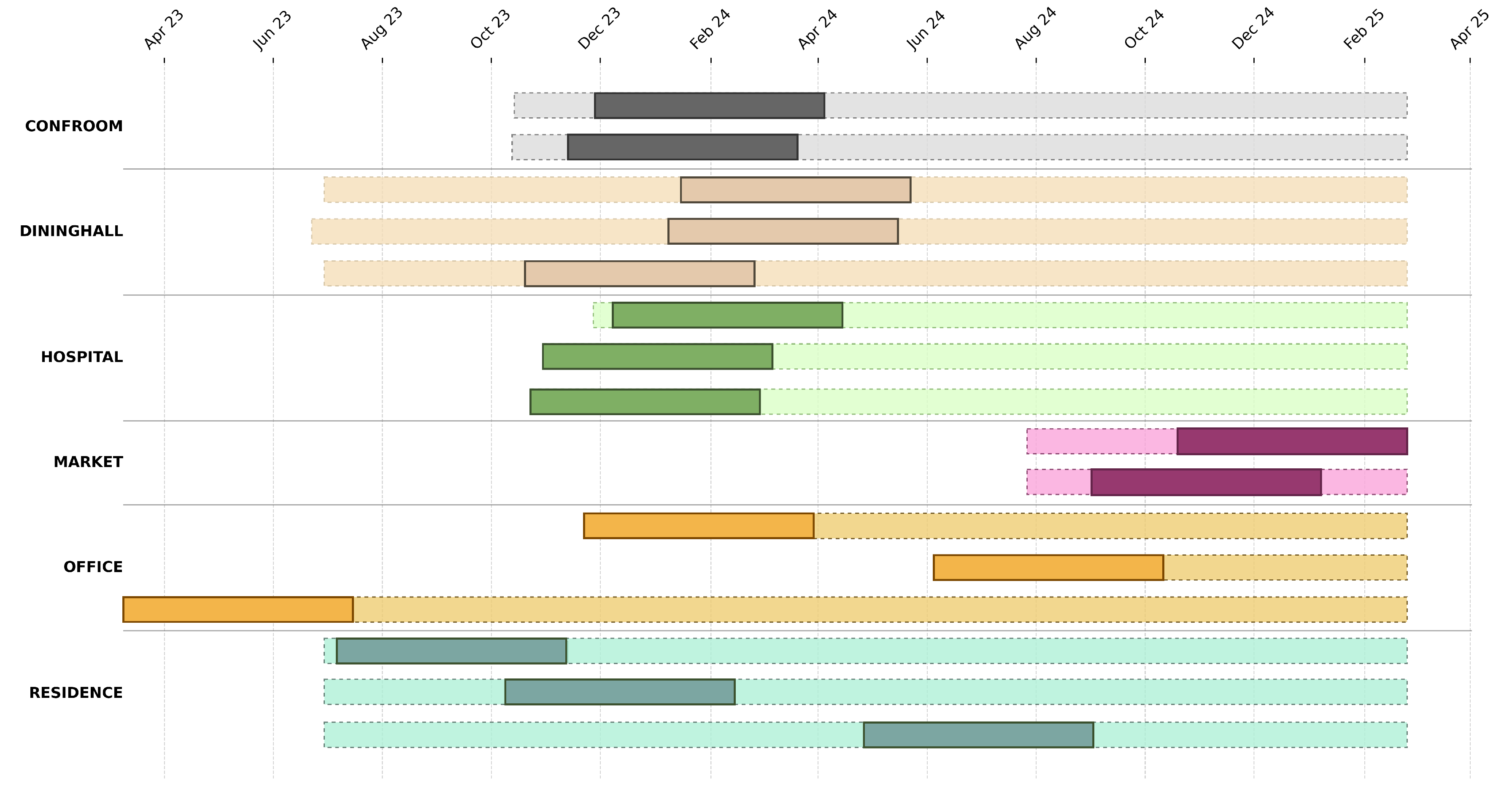
Finally,
Figure 1 shows a visual summary of the total data collection period for each device. The selected 18-week subset used in this study is highlighted in a darker segment.
2.3. Data Analysis
The study considered six representative indoor environments, each selected to capture distinct occupancy patterns and dynamic behaviors associated with CO2 concentrations. These variations are fundamental for assessing whether predictive models can generalize across different environments. A detailed description of each use case is provided below:
Conference Room (CONFROOM): Conference rooms are characterized by long periods of inactivity punctuated by short but intense occupancy during scheduled meetings or events. This typically results in rapid and pronounced increases in CO2 concentration during occupancy, followed by abrupt declines once the room is vacated or when the ventilation system effectively removes the accumulated CO2.
Dining Hall (DININGHALL): Dining halls are defined by periodic and recurring occupancy peaks, generally aligned with meal times. These peaks occur at relatively predictable times of day, but their magnitude and duration vary depending on the number of users and the day of the week. This yields a partially regular pattern (owing to its daily rhythm) that nevertheless contains variability and occasional unexpected surges.
Hospital (HOSPITAL): Hospitals are characterized by continuous occupancy because patients are present 24 h a day and healthcare staff are constantly active. This uninterrupted human presence leads to CO2 levels that remain persistently elevated throughout the day. In these environments, ventilation is typically mechanically controlled to maintain health and safety standards, which generally results in smoother concentration curves than in other use cases. In the specific hospital considered for this study, concentrations increased during the night-time period due to a lower ventilation rate, whereas levels decreased during the day thanks to more intensive ventilation. This pattern represents a different dynamic compared to the one observed in most other environments.
Food Market (MARKET): Food markets are characterized by heterogeneous and irregular occupancy, strongly influenced by external factors such as opening hours, day of the week, seasonal variations throughout the year, and even weather conditions that affect customer flow. CO2 levels may remain close to baseline values for long periods and then rise sharply with the sudden arrival of visitors. Although recurrent increases around midday and a notable rise on Saturdays can be identified in the analyzed data, the magnitude and regularity of these peaks vary considerably, reflecting the unpredictable nature of the environment.
Office (OFFICE): Offices typically follow occupancy cycles linked to working hours. Activity is concentrated mainly on weekdays, with a lower presence in the evenings and at weekends. Within the working day, however, fluctuations occur due to breaks, meetings, or hybrid working arrangements that alter the expected trends. This intermediate scenario combines regular daily cycles with occasional variability, constituting a use case with moderately stable but non-continuous dynamics.
Student Residence (RESIDENCE): Student residences are characterized by prolonged occupancy with gradual and less structured dynamics. Residents typically spend long periods in their rooms, alternating between studying, leisure, and rest. Ventilation habits are irregular, depending on window opening or the use of mechanical systems, which often leads to a gradual accumulation of CO2 over time. Unlike spaces with abrupt peaks (such as conference rooms), student residences exhibit slower yet persistent variations.
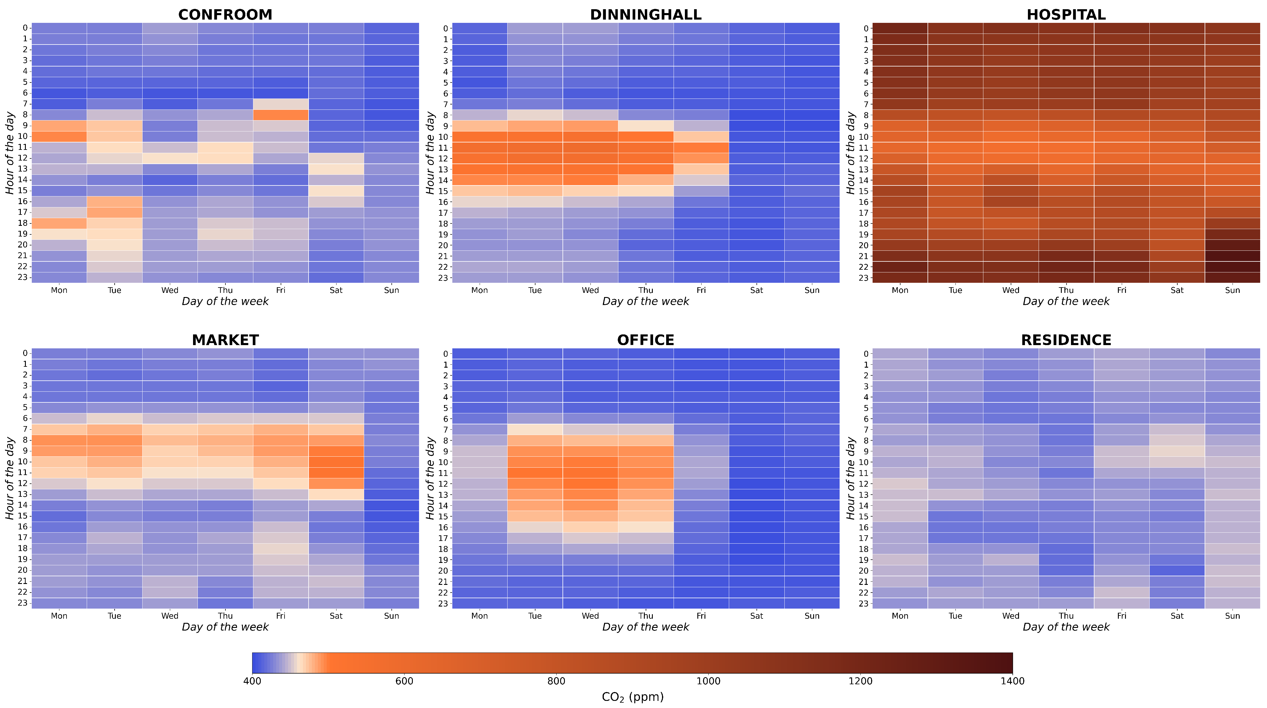
To examine CO
2 temporal patterns (as occupancy proxies) in greater detail,
Figure 2 presents weekly heatmaps of CO
2 concentration for each use case. These visualizations depict the mean concentration computed across all devices associated with the same environment, aggregated by hour of the day and day of the week over the full 18-week period. Each matrix shows the hours of the day on the vertical axis and the days of the week on the horizontal axis, with a color scale indicating CO
2 concentration in ppm. This representation facilitates the identification of recurrent occupancy-related patterns based on the typical accumulation of CO
2 associated with human presence.
Table 1 presents the basic descriptive statistics that quantify the observed patterns. In most use cases, the mean CO
2 concentration is close to the traditional baseline level of an unoccupied space (400 ppm [
6]), which is consistent with a low occupancy frequency. In contrast, HOSPITAL exhibits the opposite pattern, with substantially higher mean values over time, which supports its condition of continuous occupancy. The standard deviation provides additional insight: high values alongside means close to the baseline level, as in CONFROOM, DININGHALL and RESIDENCE, suggest sporadic but significant occupancy events, whereas OFFICE shows lower variability, consistent with its more stable daily cycles.
Overall, these observations highlight how CO2 concentrations depend on the type of space and its occupancy patterns. This relationship motivates the use-case-based analysis adopted in this work and provides the methodological basis for the forecasting approaches evaluated in the subsequent experimental section. However, because occupancy and ventilation control actions are not directly observed, these patterns should be interpreted as CO2-based proxies rather than ground-truth measurements of the underlying drivers.
3. Materials and Methods
As reported in the literature, the use of ML models can improve the forecasting of CO
2 levels compared with simpler approaches in certain specific contexts, such as schools [
16]. However, this section aims to address the stated objective: are ML models useful across multiple scenarios with different occupancy patterns?
As described in the previous
Section 2, this study considers six scenarios (CONFROOM, DININGHALL, HOSPITAL, MARKET, OFFICE and RESIDENCE), with a total of 16 deployed devices. For each device, a dataset corresponding to 18 consecutive weeks of CO
2 measurements is available, sampled at 10 min intervals, resulting in 18,144 records per device (290,304 observations in total).
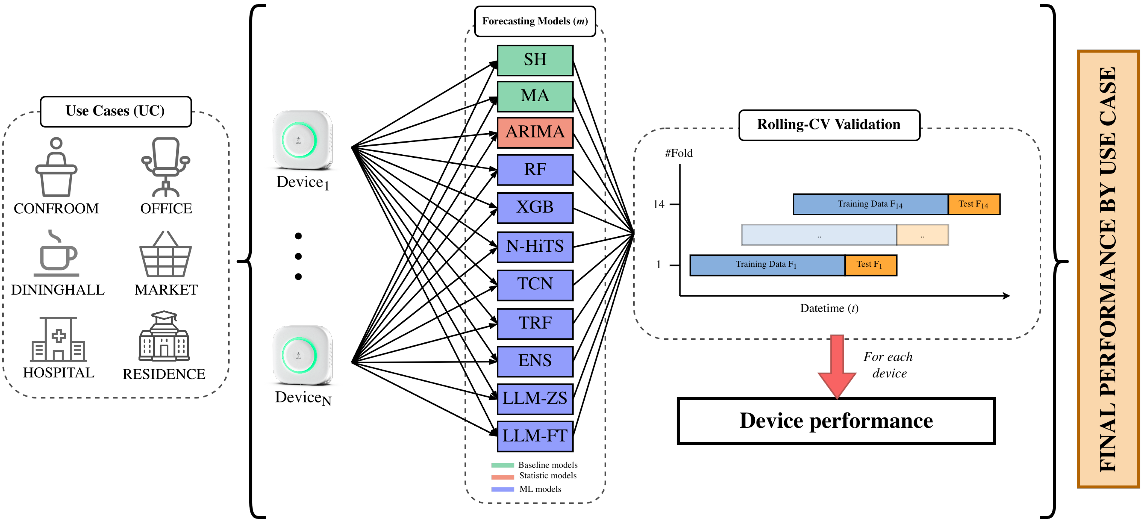
In order to have a global view of the experiment performed, the pipeline applied in this study is as follows: (i) CO
2 data are measured using the deployed devices; (ii) for each device, an 18-week consecutive subset is selected according to the criteria defined in
Section 2.2; (iii) all selected series are homogenized with a uniform 10 min sampling interval and consistent missing-data handling; (iv) temporal validation is applied independently to each device using Rolling-CV (detailed in
Section 3.4).
In each device we apply Rolling-CV to have multiple temporal folds, and each fold is split into training and validation subsets. In each fold, models are trained on the corresponding training subset and evaluated on the associated validation subset for that horizon. This produces one performance value per fold; the global performance of a model on a given device is computed as the arithmetic mean across folds.
Finally, for each prediction horizon, use-case-level performance is obtained by aggregating the device-level results of all devices belonging to the same use case. Therefore, comparative results are consistently reported by model, device, use case, and prediction horizon.
Figure 3 summarizes this methodological workflow.
3.1. Forecasting Models
We selected eleven forecasting models representing three common methodological approaches in TS forecasting: simple models, statistical models, and ML-based models. This selection covers widely used techniques in the literature and enables the comparison of approaches with different levels of complexity under a common experimental framework.
The simple-model block includes low-computational-cost methods that serve as reference baselines. The statistical-model block comprises classical approaches based on the intrinsic properties of the TS, exploiting patterns such as autocorrelation, seasonality, and trend. Finally, the ML block group methods learn patterns directly from data without explicitly imposing a parametric structure on the series, allowing them to capture complex and non-linear relationships. The models considered are described below.
3.1.1. Simple Models
Shifted model (SH): performs a constant shift of the TS itself as the forecast. The shift is determined by the prediction horizon under analysis.
Moving Average model (MA): uses a moving average of the last N CO2 values as the forecast. In this study, a 1 h window (6 measurements) is used to compute the average.
3.1.2. Statistical Models
Autoregressive Integrated Moving Average model (ARIMA) [
21]: a model widely used in the literature. We used an autoARIMA implementation provided by the DARTS library [
22] to estimate the parameters.
3.1.3. ML-Based Models
Within this framework, four model categories were considered: classical ML, deep learning (DL) architectures, ensembles, and foundation models.
Classical ML Models
This category includes well-established learning algorithms widely used in general ML and common in pollutant forecasting literature, where they have demonstrated strong performance in TS prediction [
8]. The models selected were:
DL Models
This group comprises neural architectures designed to capture non-linear and temporal relationships by leveraging established DL designs for sequence modeling. The models selected were:
Neural Hierarchical Interpolation for TS Forecasting (N-HiTS) [
25].
Temporal Convolutional Network (TCN) [
26].
Ensembles
This category combines forecasts from multiple models to leverage complementary strengths and improve forecasting accuracy in TS prediction [
28,
29].
Foundation Models
This category includes models from the Chronos family [
30,
31], which are TS foundation models that reuse language-model architectures (T5) but are pretrained on numerical TS, not on natural-language text. Chronos converts a real-valued series into discrete tokens via per-window scaling and quantization, so forecasting becomes next-token prediction optimized with cross-entropy. The models are pretrained on a large and diverse corpus of publicly available real-world TS datasets, complemented with synthetic series generated via Gaussian processes to broaden the range of trends/seasonalities and improve zero-shot generalization. This combination (tokenization + probabilistic next-token modeling + large multi-domain pretraining) largely explains the strong performance observed even without task-specific training. Two Chronos models integrated into AutoGluon [
32] were evaluated:
Chronos-T5 Tiny zero-shot (LLM-ZS): Deployed in a strict zero-shot setting. This model generates forecasts relying exclusively on its pre-trained general knowledge, without being exposed to the training partition of the specific target buildings.
Chronos-T5 Tiny fine-tuned (LLM-FT): Extends the pre-trained base model by incorporating a fine-tuning stage on the specific historical data of the target buildings, allowing the model to adapt its weights to the particular dynamics of each use case.
A general configuration was employed across model training, consisting of a window size of 144, 200 training epochs, a batch size of 256, and a learning rate of
using the Adam optimizer with a dropout probability of
. No hyperparameter tuning was performed. For Classical ML and DL models, normalization of the input values to the interval
was applied as a preprocessing step. The model-specific configurations are summarized in
Table 2.
3.2. Prediction Horizons
In the TS forecasting literature, it has been observed that, particularly for short-term prediction tasks, simple models with low computational cost can outperform more complex alternatives [
33,
34]. This phenomenon remains an open question in the field, highlighting the importance of understanding model behavior across different forecast horizons. As the prediction horizon increases, the problem becomes more complex to model.
In this context, it is relevant to explore whether simple models can still provide accurate forecasts of CO2 levels as the horizon extends and whether they may even outperform more sophisticated approaches under certain conditions.
To address this, the present study evaluates model performance across multiple forecast horizons, examining CO2 predictions at varying temporal distances. Specifically, the following horizons are considered throughout the experimental setup: (10 min ahead), (1 h), (2 h), and (4 h).
3.3. Input Configuration and Sliding Window Strategy
We adopt a single data formation strategy to compare the 11 models on equal terms. Forecasting is univariate: only historical CO
2 observations are used as input, with no auxiliary covariates or future information. All series are resampled to a uniform 10 min interval (
Section 2.2), so the temporal resolution is consistent across use cases and models.
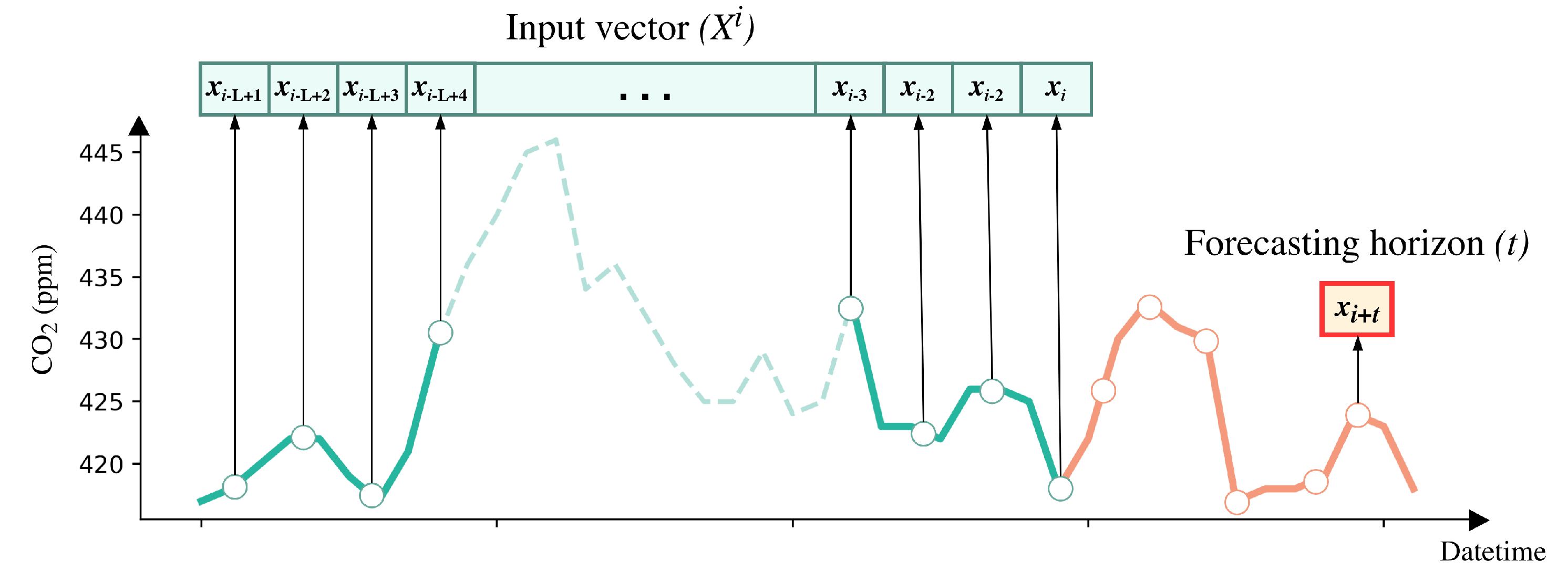
Input Vector Construction: The input for each model consists of a fixed look-back window of
historical observations. Given the 10 min resolution, this window represents the preceding 24 h of CO
2 dynamics. At time index
i, the input vector is defined as
, where
denotes the CO
2 concentration at
i. For a given forecasting horizon
t, the associated target value is
. This configuration is illustrated in
Figure 4 for the case
(1 h ahead). The same window length is used for all models, including foundation models, where it corresponds to the input context length.
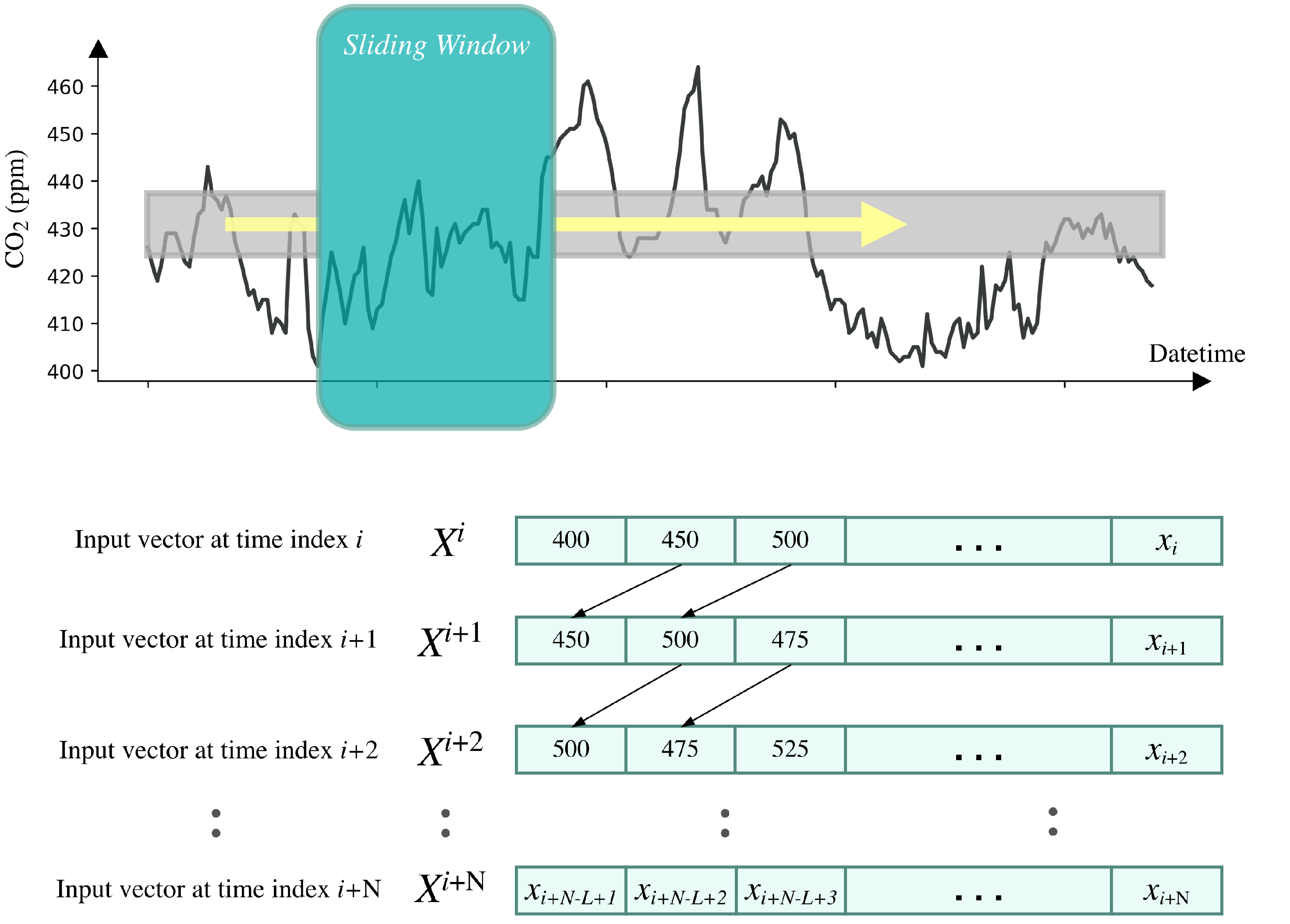
Sliding Window Procedure: For each device, a sliding window iterates across the time series to generate the full dataset (
Figure 5). At each time index
i, a new input-target pair
is constructed. The window advances by one time index (10 min) at each iteration, producing a new sample until the end of the available data.
Forecasting Strategy: A direct forecasting approach is adopted. Instead of recursive multi-step prediction, a separate model instance is trained for each target horizon
defined in
Section 3.2. Each model learns to map the input vector
to its corresponding target
for the specific horizon under analysis.
3.4. Validation
In this study, the Rolling-CV temporal cross-validation technique [
35] was used in TS problems to generate multiple training and test splits. Its purpose is to evaluate the model across different time periods and to avoid dependence on a single test interval.
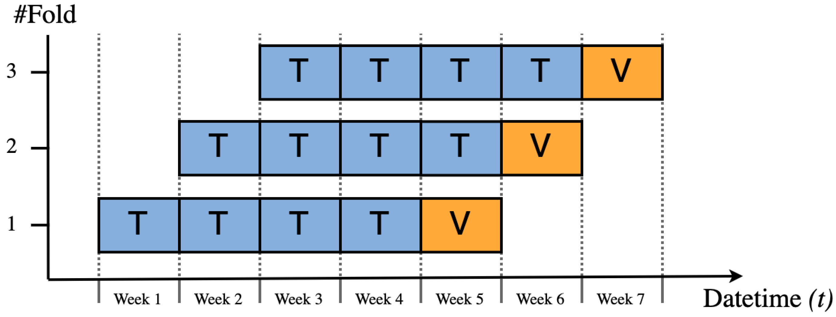
Rolling-CV was applied independently to each device using an overlapping variant in which the validation set from each iteration is subsequently incorporated into the training set. From the complete dataset of measurements for each device, multiple temporal subsets (folds) were generated, maintaining a fixed proportion of 80% of the data for training and the remaining 20% for validation in each split.
Given that an 18-week consecutive dataset is available for each device, a total of 14 folds were generated per device. Each fold follows a five-week configuration, in which the first four weeks are used for training and the fifth week for validation.
Figure 6 shows an illustrative scheme of the first three folds generated under this configuration.
3.5. Error Metrics
In IAQ-related forecasting problems, the most commonly used metrics in the literature are RMSE (Root Mean Squared Error), followed by R
2 (coefficient of determination), MAPE (Mean Absolute Percentage Error), MAE (Mean Absolute Error), and MSE (Mean Squared Error). However, metrics such as RMSE, MAE, and MSE, despite being traditional measures widely used in ML, are scale-dependent. This hinders the comparison of model performance when models are trained on datasets of different magnitudes [
8], representing a significant challenge when comparing models across datasets with different scales. Therefore, it is recommended to select non-scale-dependent metrics for model comparison [
4]. Given that CO
2 levels and data scales in this study vary depending on the use case, we selected two complementary metrics based on MAE but measuring different aspects of model performance: MAPE and
.
MAPE [
36] measures the percentage error of predictions. Given two TS, it is defined as
where
and
denote the observed and predicted values at time step
i, respectively, and
N is the number of observations.
The
quantifies the relative improvement of the proposed models with respect to a reference baseline model, which, in this study, is the Shift model (SH). It is defined as
where
and
represent the MAE [
37] of the evaluated model and the reference model, respectively, calculated as
In this context, an indicates that the proposed model outperforms the SH model (achieving higher accuracy), whereas a value implies inferior performance.
To evaluate the overall performance, we followed a two-step aggregation process. First, the performance of a model for a specific device is calculated by averaging the results obtained across the 14 folds. Then, the performance of a model for a given use case is determined by the arithmetic mean of the performance of all devices belonging to that use case. This methodology provides a global performance measure for each use case, model, and prediction horizon.
4. Experimental Results
After completing the experimental process across the sixteen devices included in this study, the results for the proposed models (SH, MA, ARIMA, RF, XGB, N-HiTS, TCN, TRF, ENS, LLM-ZS, LLM-FT) were obtained for each use case described in
Section 2.
Table 3 presents the overall MAPE values for each use case in the evaluated prediction horizons (
,
,
and
), averaged across devices. For completeness, per-device MAPE values and standard deviation across validation folds are reported in
Table A3 and
Table A4.
The analysis of
Table 3 reveals a significant disparity in prediction difficulty across use cases, with the HOSPITAL scenario exhibiting the highest systematic error. While in environments such as the RESIDENCE or OFFICE, long-term MAPE values (
) remain notably low (ranging between 3% and 4.5%), in the HOSPITAL, the error surges above 28%.
Across prediction horizons, a consistent pattern is observed: SH and ARIMA dominate at short horizons, whereas their error increases more sharply as the horizon extends. At
, SH and ARIMA almost always achieve the best results (bolded in
Table 3). By contrast, at
their MAPE increases substantially relative to other approaches. At longer horizons (
and
), ENS and LLM-FT emerge as the most robust solutions across several use cases. In scenarios such as the DININGHALL, MARKET, and OFFICE, ENS consistently minimizes error at these horizons, while Classical ML (RF and XGB) and DL models tend to present slightly higher errors.
Regarding foundation models, a clear performance gap is observed between LLM-ZS and LLM-FT across multiple scenarios and horizons. Nevertheless, LLM-ZS outperforms Classical ML and DL models (e.g., RF, XGB, and N-HiTS) in several cases. For instance, in CONFROOM and RESIDENCE, zero-shot yields lower error than some trained architectures.
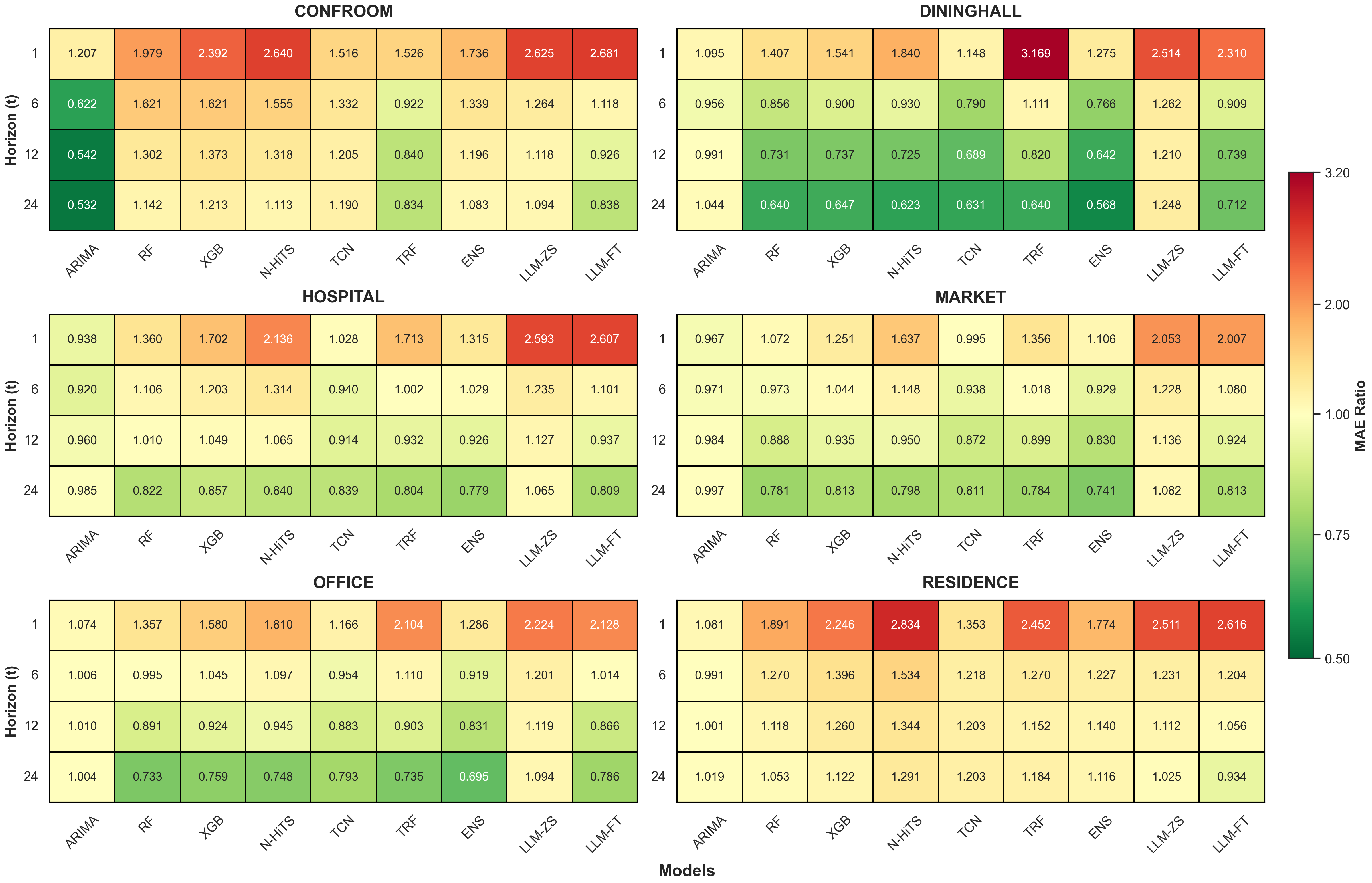
To quantify the extent to which ML models improve or degrade relative to the simplest baseline (SH), we computed the
in
Table A2 (from MAE values in
Table A1).
Figure 7 presents a heatmap where green shades indicate improvement over SH and red shades indicate degradation.
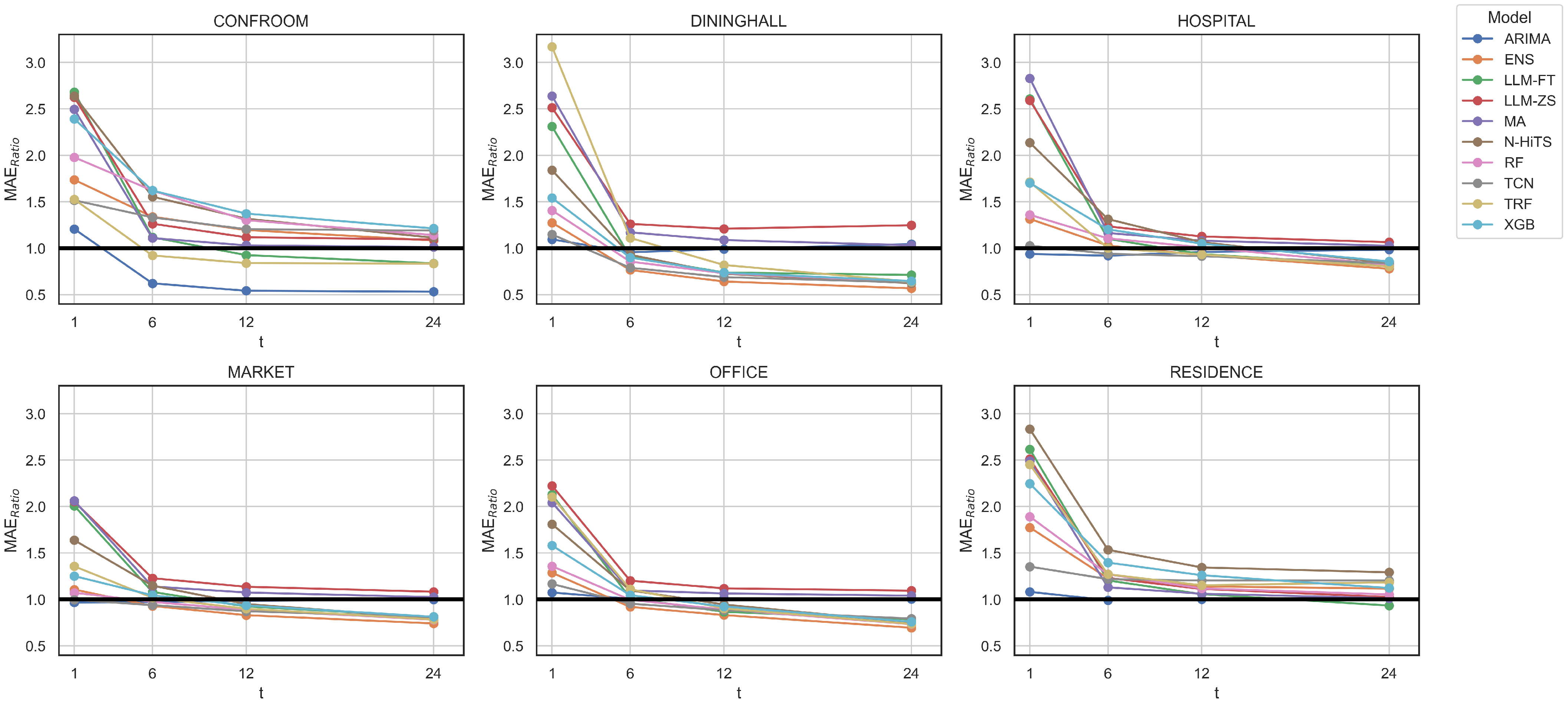
Figure 8 shows the evolution of
across horizons for each use case, with a horizontal threshold at
.
Both figures indicate that, at short horizons, improvements over SH are limited: many complex architectures have at . As the horizon increases, decreases in most use cases, and at and , ENS and LLM-FT frequently fall below the unit threshold. This trend is less pronounced in CONFROOM and RESIDENCE, where SH remains competitive across most horizons.
These results suggest that the HOSPITAL’s temporal dynamics are more challenging for all algorithm categories, potentially due to the continuous-occupancy regime. The short-horizon dominance of SH and ARIMA is consistent with strong short-term autocorrelation in indoor CO2, where concentrations typically evolve gradually. Conversely, the longer-horizon advantage of ENS and LLM-FT indicates that approaches capable of capturing broader temporal structure become more beneficial as persistence weakens.
For the foundation models, the observed gap between LLM-ZS and LLM-FT supports the role of fine-tuning for capturing building-specific dynamics, especially in complex scenarios and longer horizons, as also reported in [
31]. At the same time, the competitive performance of LLM-ZS in selected scenarios suggests that pretrained temporal representations can be strong even without exposure to target-building training data.
Statistical Test
In order to evaluate the statistical significance of performance differences among models, a hierarchical statistical evaluation was adopted across the sixteen devices at each horizon, inspired by the methodology described in [
38]. In this analysis, each device constitutes one observational unit (block) using the per-device mean error average across the 14 rolling-CV folds. Folds are not treated as independent observations due to temporal overlap; comparisons are therefore paired at the device level. As illustrated in
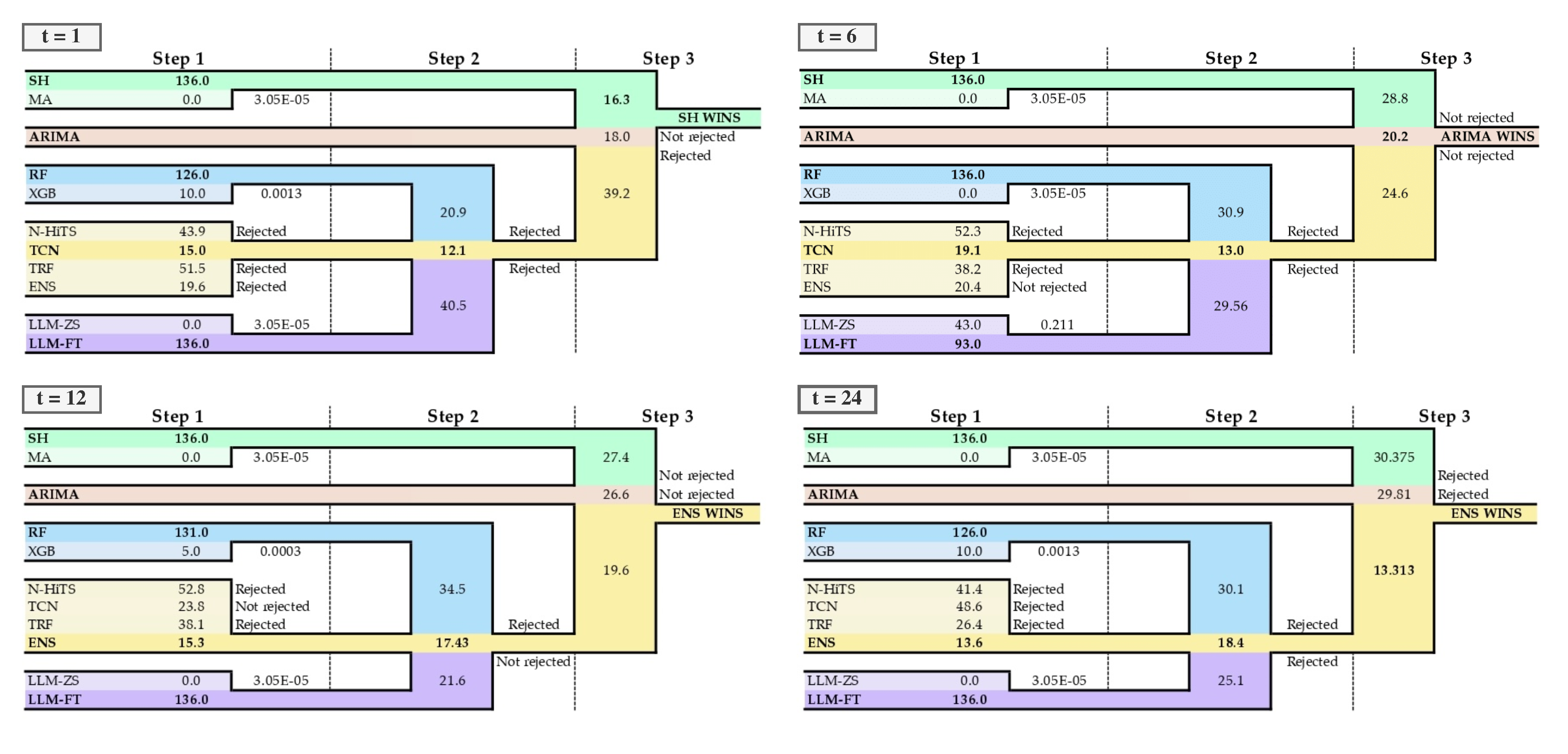
Figure 9, this evaluation is structured as a multi-step tournament designed to identify the most robust forecasting approach. The process began by categorizing models into five distinct families (baselines, statistical methods, classical ML models, DL architectures, and LLMs) and performing an intra-family comparison to select the best representative for each group. Subsequently, the winners of the learning-based families were compared to determine the superior “Best ML” approach. In the final stage, this top ML model was compared against the best baseline and the best statistical method to determine the global winner.
Regarding the statistical tools employed to execute this protocol, different non-parametric tests were applied depending on the comparison type. When comparing a group of methods (more than two), the Aligned-Friedman test [
39] was used, followed by Holm’s post hoc test [
40] to identify significant differences. Conversely, for pairwise comparisons, the Wilcoxon signed-rank test [
41] was employed. Adjusted p-values (
) were used to determine whether to reject the null hypothesis of equivalence between methods. Note that regarding the interpretation of results, lower ranks imply better performance for Friedman, while higher rank sums indicate superiority for Wilcoxon. This statistical protocol is widely recommended for ML model comparisons in the literature [
16,
42,
43,
44,
45].
Based on the results shown in
Figure 9, a clear transition is observed regarding the prediction horizon. At the shortest horizon (
), baseline models, specifically SH, demonstrate statistical superiority, outperforming more complex architectures in the final comparison. However, as the horizon extends, the trend reverses: the “Best ML” branch consistently prevails over the “Baselines” branch. This statistical validation confirms the findings from the MAPE analysis, proving that while simple heuristics suffice for immediate next-step predictions, learning-based approaches are statistically superior for capturing longer-term dependencies.
Nevertheless, the fact that a specific model wins the final round of the hierarchical test does not necessarily imply it is strictly superior to every other model in its category, but rather that its family performs better on average. To address this, we conducted an auxiliary analysis to determine if the top-performing model is statistically distinguishable from the remaining architectures in the family. Only the cases where an ML model emerged as the winner (
and
) are considered, because SH (
) was already compared against MA, and ARIMA does not have any other method in its family.
Table 4 presents the results of the Wilcoxon signed-rank test, comparing the “Best ML” model (Control) against the other candidates.
As shown in
Table 4, ENS demonstrates a statistically significant advantage over individual architectures in most pairwise comparisons. A notable exception, however, is observed in the comparison with LLM-FT. Across both horizons, we fail to reject the hypothesis of equivalence, indicating a lack of statistical evidence for ENS’s superiority over LLM-FT. These results underscore the competitiveness of the LLM-FT approach, which effectively matches the performance of top-tier ensemble strategies in challenging long-term scenarios.
Finally, it is important to interpret these statistical results as a global assessment of performance consistency rather than a universal verdict. While the hierarchical tests identify the models that are most robust on average across the entire dataset, the detailed analysis in
Section 4 revealed that the optimal forecasting strategy is highly dependent on the specific use case. Consequently, the statistical superiority reported in this section reflects the generalizability of the models across diverse conditions, but it does not preclude that, in specific environments, alternative architectures may yield better results depending on local dynamics.
5. Discussion
The analysis of the results across six heterogeneous use cases reveals that there is no universal prediction strategy for forecasting CO2 indoors. Unlike controlled environments, contextual variability dictates model performance, leading to several critical findings that qualify and expand upon previous literature.
A clear dichotomy is observed based on the structure of occupancy. In spaces with unstructured and sporadic occupancy (CONFROOM, RESIDENCE), CO2 levels remain close to the baseline (400 ppm) for long periods. In these scenarios, deploying complex DL models represents an inefficient use of computational resources; the SH model is not only competitive but also frequently outperforms deep architectures in short horizons. Conversely, in cyclic scenarios (OFFICE, DININGHALL, MARKET), the temporal structure is rich enough for ML models—specifically ENS and LLM-FT—to statistically outperform baselines in the long term (), capturing weekly and hourly patterns that escape simple heuristics.
A critical finding, often overlooked in IAQ benchmarks, is the contrasting performance observed between use cases. While the MAPE remains low (3–5%) in OFFICE or RESIDENCE, it exceeds 30% in the HOSPITAL setting for all models, including LLMs. This systematic difference suggests that the historical CO2 TS alone is insufficient to capture the dynamics of continuously occupied, mechanically ventilated environments. The inclusion of exogenous variables, such as HVAC schedules, occupancy counts, or outdoor weather conditions, could potentially improve forecasting accuracy in such complex scenarios.
These findings have direct implications for the extrapolation of results from school environments. The trend observed in schools—where ML models outperform simple baselines as the prediction horizon increases—is validated in structured cases like OFFICE and DININGHALL but is not observed in sporadic spaces where simplicity prevails. Therefore, a one-size-fits-all model strategy is unfeasible.
The incorporation of Foundation Models and ensemble approaches represents a positive advancement over the benchmark established in schools. ENS and LLM-FT have demonstrated highly competitive performance in long-term predictions, outperforming the rest of the evaluated models at extended horizons. Statistical tests confirm that both approaches achieve equivalent performance, with no significant differences observed between them at and . Notably, LLM-ZS, despite not being the best-performing model overall, achieved competitive results without any local training, often surpassing trained models such as N-HiTS and XGB in several use cases. This generalization ability makes LLM-ZS a valuable candidate for deployment in scenarios with limited or no historical data available for model training, after which a transition to locally trained ensembles (ENS or LLM-FT) could optimize computational cost without sacrificing accuracy.
6. Conclusions and Future Work
This study presents a comprehensive methodological framework for CO2 forecasting using data from low-cost IoT sensors across six diverse indoor environments with heterogeneous occupancy dynamics, addressing a critical gap in indoor air quality research. By combining robust validation, statistical analysis, and scale-independent metrics across multiple prediction horizons and use cases, it establishes a reference benchmark for evaluating model performance under real-world contextual variability.
Furthermore, we evaluate the application of Foundation Models to indoor pollutant forecasting. While these models have recently revolutionized general ML tasks, their adaptation to time series forecasting remains nascent. This study provides a primary quantitative benchmark of their performance against standard ML approaches across multiple indoor scenarios, opening a promising research avenue in the IAQ domain.
By extending the benchmarking framework previously applied in schools [
16] to these diverse indoor environments, our findings confirm that the optimal forecasting strategy is strictly dependent on the prediction horizon and the specific occupancy regime. Consistent with previous findings, simple and statistical models (SH, ARIMA) dominate in short-term horizons (
), driven by the strong short-term autocorrelation inherent to indoor CO
2 dynamics. Conversely, as the horizon extends to medium- and long-term ranges (
,
), ML models—particularly ENS and LLM-FT—demonstrate superior robustness, exhibiting a more gradual performance degradation than baseline approaches. Statistical tests confirm this general trend; however, the analysis reveals that model performance is conditioned by specific use cases and local CO
2 patterns, necessitating a preliminary analysis of the target space’s dynamics before deploying a forecasting solution.
Overall, this research provides evidence on the generalizability of performance patterns across use cases, while showing clear boundaries and context dependence. Beyond offering a tailored solution for specific environments, this study serves as a guideline for future IAQ research in different indoor settings by clarifying which findings from educational settings [
16] replicate in other domains and which do not.
Building upon these findings, several future research directions emerge. This study has primarily focused on forecasting performance across different models and use cases. However, transitioning from research to production deployment requires addressing additional practical considerations, including model deployment costs, inference time, training time, and the need for periodic retraining. Future work should systematically evaluate these operational aspects to provide a comprehensive framework for real-world implementation.
Beyond these operational considerations, a pervasive challenge in the literature is the scarcity of large-scale, uninterrupted datasets from uncontrolled environments, which complicates extensive validation. While future work under project [
19] aims to bridge this gap by expanding data collection, we also propose a complementary research avenue focused on model generalization to mitigate data dependence. Specifically, we will investigate both intra-use-case unification (e.g., a single model for all offices) and inter-use-case transferability (e.g., applying office-trained models to dining halls with similar cyclic patterns). Validating whether models can be successfully transferred between environments with shared behavioral characteristics would represent a significant industrial breakthrough, effectively bypassing the bottleneck of obtaining extensive historical data for every new deployment.