Predictive Monitoring of Wage-Band Classification in GOSI Data with Leakage Control and Out-of-Time Validation

Highlights

What are the main findings?

• We develop a reproducible, leakage-controlled predictive monitoring pipeline using quarterly GOSI administrative releases (Q1–Q3 2024) to classify aggregated contributor groups into low/medium/high wage bands.
• Under leakage control, the models achieve stable performance across releases, with most errors concentrated between adjacent wage bands; out-of-time validation indicates that predictive skill transfers across quarterly updates.

What are the implications of the main findings?

• Quarterly administrative releases contain persistent actionable signals that can support forecasting-oriented labor-market surveillance and early-warning dashboards without using salary-derived inputs.
• Probability calibration improves the reliability of risk scores for threshold-based monitoring decisions, supporting more consistent operational triage across new quarterly releases.

Abstract

Timely labor market monitoring is essential for policy design and operational planning, yet annual reports can mask turning points and subgroup heterogeneity. This paper develops a reproducible monitoring and prediction framework using administrative statistics from the General Organization for Social Insurance (GOSI) in the Saudi Open Data Portal. We document descriptive patterns in formal participation and insurable wages, including age-group dispersion, stable correlation structure, and explicit handling of an anomalous wage release and limited missing wage entries. We then formulate from non-salary administrative descriptors. Under leakage control, Random Forest models achieve accuracy around 0.71 across releases. Most errors are concentrated between adjacent wage bands, which is consistent with threshold discretization of a continuous wage distribution. To support operational deployment, we add out-of-time validation across releases and probabilistic assessment, showing that predictive skill transfers across updates and that calibration improves the reliability of probability scores for monitoring thresholds. Overall, the results indicate that administrative releases contain persistent actionable signals for wage segmentation without salary-derived inputs, supporting forecasting-oriented surveillance and early-warning dashboards.

1. Introduction

High-frequency monitoring of labor market conditions is increasingly important for policy design, operational planning, and near-term assessment of reforms. Annual labor reports remain essential for benchmarking long-run trends, but can mask within-year turning points, compositional shifts across demographic groups, and short-horizon wage dynamics that matter for timely intervention. From a forecasting perspective, the value of higher-frequency information is not only descriptive; it can enable practical predictive monitoring, support nowcasting-style updates as new releases arrive, and provide a disciplined foundation for quarter-ahead forecasting once longer quarterly histories become available. For such uses, it is not sufficient to report within-sample or within-quarter accuracy; a monitoring system must also demonstrate operational validity under realistic deployment conditions, namely, that models trained on one release remain informative when applied to the next release and that probability scores used for alerting and triage are well-calibrated.

Saudi Arabia offers a particularly relevant context for such analysis. Vision 2030 programs and labor market regulations exhibit within-year evolution, and their effects may appear first as changes in formal participation and insurable wages across sectors, regions, and demographic categories. However, empirical work is often constrained by limited frequency, restricted access, or non-comparable definitions across sources. In this paper, we leverage quarterly administrative statistics from the General Organization for Social Insurance (GOSI) obtained from the Saudi Open Data Portal. These statistics summarize formal labor market participation (contributors) and wage indicators (average insurable wage) over Q1–Q3 2024. The releases provide a standardized and repeatable view of the insured workforce across a rich set of aggregated categories (e.g., office/region, economic activity, age group, legal entity type, nationality, and gender where available), making them suitable for systematic quarterly monitoring and for evaluating whether signals transfer across releases.

The central methodological objective of this study is to move beyond reporting descriptive quarter-to-quarter changes and develop a reproducible prediction framework that can be executed each quarter under realistic information constraints. Specifically, we formulate a supervised classification task in which each aggregated contributor group is assigned a salary class (Low/Medium/High) derived from the reported average insurable wage, then evaluate whether wage classes can be predicted from non-salary administrative descriptors alone. This framing aligns with forecasting practice in two ways: it produces an operational early-warning signal for segmentation, and it establishes a baseline predictive layer that can later be extended into time series forecasting once additional quarters are accumulated. To strengthen its operational relevance, we additionally evaluate how models behave under out-of-time quarter-to-quarter deployment. Because monitoring decisions often rely on predicted probabilities and threshold rules rather than hard labels alone, we also assess probabilistic skill and calibration.

A key practical challenge in wage prediction is information leakage, in which models can appear highly accurate if they inadvertently use variables that encode the target directly or through deterministic transformations. To ensure credible evaluation, we adopt a strict leakage control protocol in which the continuous wage value is used only to construct the label; together with wage-derived ratios, it is excluded from the feature set. We then compare an interpretable Decision Tree baseline against a Random Forest ensemble using a consistent stratified train–test evaluation within each quarter. In addition, because administrative releases may contain reporting artifacts, we explicitly document and handle data quality issues, including the Q1 wage anomaly and a small number of missing wage entries in Q2 and Q3; we emphasize interpretations that remain robust to these limitations. Building on these within-quarter results, we further introduce an operational validation layer that tests quarter-to-quarter generalization, examines error structure under distribution shift using out-of-time confusion matrices, and evaluates calibration and proper scoring rules to support decision-relevant monitoring.

This study makes several contributions that are directly relevant to forecasting. First, to the best of our knowledge, it is among the first works to operationalize the publicly available quarterly GOSI Open Data releases into a complete end-to-end predictive monitoring pipeline that is reproducible, leakage-safe, and accompanied by explicit operational validation across quarters. Second, it provides a transparent empirical characterization of quarterly labor-market patterns in Saudi Arabia (contributors, wage distributions by age group, and correlation stability across quarters), clarifying what higher-frequency administrative monitoring reveals beyond annual summaries. Third, it delivers interpretable and benchmarkable predictive baselines (Decision Tree and Random Forest) for salary class prediction under realistic constraints, with diagnostic outputs that support policy-facing interpretation. Fourth, it extends evaluation beyond within-quarter splits by introducing out-of-time validation and probabilistic calibration analysis, thereby aligning model assessment more closely with forecasting practice and the requirements of real monitoring dashboards. Finally, the paper outlines a clear path from quarterly predictive monitoring toward genuine forecasting extensions, including nowcasting updates, multi-step quarter-ahead forecasts with uncertainty quantification, and hierarchical forecasting across region–sector–age aggregations once longer quarterly histories become available.

The remainder of the paper is organized as follows. Section 2 reviews prior work on forecasting-oriented monitoring frameworks and hybrid statistical–machine learning approaches, and clarifies how our quarterly leakage-controlled administrative pipeline complements this literature. Section 3 describes the GOSI datasets, preprocessing steps, and data-quality considerations. Section 4 reports descriptive quarterly evidence on contributors, wages, age group distributions, and correlation structure. Section 5 formulates the salary class prediction task, details the leakage-controlled feature set, and evaluates Decision Tree and Random Forest models under within-quarter splits. Section 8 introduces the operational forecasting-oriented validation layer, including out-of-time quarter-to-quarter testing, error structure diagnostics, and calibration and probabilistic skill evaluation. Optional unsupervised segmentation is discussed in Section 6, and an interpretation-only LLM-assisted layer is documented in Section 7. Section 9 summarizes implications, limitations, and generalizability. Finally, Section 10 concludes with forecasting-oriented directions for future work.

2. Related Work

The present study sits at the intersection of forecasting methodology, high-frequency monitoring, and administrative data analytics. Two strands are particularly relevant for positioning the contribution first as forecasting-oriented model design and validation under operational constraints, and second as empirical labor or pension research that motivates why subgroup heterogeneity and short-horizon shifts matter for policy. A third smaller strand relates to predictive modeling on administrative or registry-style data, where leakage control and reproducibility are central concerns. Across these strands, the common limitation is that many studies either (i) focus on forecasting of a single time series with rich histories but limited subgroup structure, or (ii) study retirement and pension outcomes with strong behavioral and institutional framing but without a reusable high-frequency predictive monitoring pipeline. Our work addresses this gap by operationalizing quarterly administrative releases into a leakage-controlled predictive segmentation framework and validating it in an out-of-time deployment-like setting that is aligned with forecasting practice. Recent labor market nowcasting and administrative data monitoring research highlights that deployment validity (out-of-time generalization) and calibrated probabilities are critical when using high-frequency releases for decision-making. In this spirit, our contribution moves beyond descriptive monitoring by combining leakage control, quarter-to-quarter validation, and calibration within a reproducible pipeline.

A first relevant strand is the growing body of forecasting work that combines classical time series models with machine learning to improve predictive performance, typically by leveraging longer historical sequences for a well-defined target series. Wu et al. [1] proposed a hybrid ARIMA–LSTM model optimized with a metaheuristic (GWO) to forecast the VIX, illustrating how hybridization can reduce model mis-specification risk when nonlinear patterns coexist with linear dynamics. Kotsompolis et al. [2] similarly combined ARIMA with machine learning components (e.g., XGBoost and LSTM) for carbon price forecasting, emphasizing the value of model ensembles and hybrid architectures in volatile markets. Su et al. [3] focused on SARIMA prediction in a managerial setting where conservative assessments are needed, highlighting a practical decision-oriented framing and the importance of producing forecasts that remain credible under uncertainty. These contributions illustrate two key expectations from forecasting outlets: methodological discipline in evaluation, and a clear link between predictive outputs and decision-making. At the same time, they predominantly address forecasting problems in which the target is a time series with a sufficiently long history, whereas the quarterly GOSI Open Data releases studied here yield a short horizon thus far (Q1–Q3 2024) and are naturally organized as repeated cross-sections over rich administrative categories rather than as a single long univariate sequence. This creates a methodological mismatch for standard time series forecasting, and motivates our design choice to begin with leakage-safe predictive monitoring and out-of-time quarter-to-quarter validation as a bridge towards future nowcasting and multi-step forecasting once longer quarterly histories become available.

A second strand concerns retirement, pensions, and labor market outcomes, where heterogeneity across subgroups is central to interpretation and timing matters for policy. Casas and Román [4] examined early retirement and automation-related considerations, illustrating that aggregate outcomes can conceal important differences across individuals and contexts. Schmied [5] studied the replacement rates required to maintain income satisfaction through retirement and found income dependence, reinforcing the idea that distributional and subgroup-aware perspectives matter. Cross-country variation in retirement behavior and occupational structure was emphasized by Sauré et al. [6], while health and life expectancy drivers of pension claiming were addressed by Aakvik et al. [7]. Survival-to-retirement inequalities by socioeconomic status were forecasted in a demographic context by Strozza et al. [8]. Policy and institutional effects were further highlighted by Hernæs et al. [9], who studied pension reform impacts on employment, retirement, and disability claims. Parallel work has investigated participation and decision-making in pension systems using modern data-driven methods; examples include Verberi and Kaplan [10], who employed machine learning to study participation in the private pension system in Türkiye, and Szakadatova et al. [11], whose focus was on behavioral biases in pension saver investment decisions. Additional institutional and portfolio perspectives include pension provision in sector-specific contexts such as farming [12], pension funds and climate strategies [13], and pension fund liquidity and cash holdings [14]. Finally, Ye et al. [15] connected cognitive constraints and retirement planning to downstream economic behaviors, again emphasizing heterogeneity in decision-making and outcomes. Collectively, this literature establishes strong motivation for subgroup-aware monitoring: labor-market and retirement outcomes depend on age, occupation, institutional settings, and behavioral drivers, with policy-relevant signals often emerging first in specific segments rather than in aggregates. However, these studies typically do not operationalize a reproducible high-frequency administrative monitoring workflow that can be re-run each quarter from a public release, and lack strict leakage control and validation designed to resemble real deployment conditions. In other words, the pension and retirement literature clarifies why segmentation and heterogeneity matter, but rarely provides an end-to-end quarterly pipeline for predictive monitoring of wage-related segmentation using administrative aggregates.

A third strand relates to predictive analytics on administrative or registry-style data and the associated risks of target leakage and overly optimistic evaluation. Mou et al. [16] used mined patterns from health records and socioeconomic data to predict educational achievement, illustrating the appeal of high-dimensional administrative sources for supervised learning. However, administrative datasets frequently contain variables that can directly encode the target or act as deterministic proxies, making leakage control critical for credible out-of-sample evaluation. This issue is especially salient in wage-related modeling, where wage-derived fields can trivially reconstruct wage-based labels. Our framework addresses this by enforcing a strict leakage protocol in which the continuous wage is used only for label construction and is excluded from the feature set, together with wage-derived ratios. Moreover, we extend beyond within-quarter random splits by adding out-of-time validation that trains on one quarter and tests on the next quarter, which better approximates operational use when a new quarterly release arrives. This validation design aligns more closely with forecasting expectations, where the relevant question is not only whether a model fits within-sample patterns but whether it generalizes to the next period under realistic information constraints.

Therefore, the main limitation emerging from the reviewed literature is a gap between forecasting methodology, which is typically evaluated on long univariate or low-dimensional time series, and policy-motivated labor or pension analyses, which emphasize heterogeneity but often lack a reproducible quarterly predictive pipeline and deployment-like validation. Our contribution is to bridge this gap in the context of Saudi Arabia by operationalizing quarterly GOSI Open Data releases into a reproducible monitoring and prediction framework that is leakage-safe, segment-aware, and explicitly validated in an out-of-time setting. The framework produces interpretable baselines and probabilistic reliability diagnostics suitable for early-warning dashboards while remaining extensible towards nowcasting and multi-step forecasting with uncertainty quantification and hierarchical aggregation as additional quarters become available.

3. Data and Preprocessing

3.1. Data Source and Coverage (Q1–Q3 2024)

This study relies on quarterly administrative statistics from the General Organization for Social Insurance (GOSI), obtained through the Saudi Open Data Portal. The portal provides aggregated records that summarize labor-market participation and wage indicators across Saudi Arabia for each reporting quarter. We focus on the first three quarters of 2024 (Q1–Q3 2024), which enables short-horizon monitoring of changes in formal employment participation and insurable wage levels during the year.

The data were downloaded as separate files for each quarter and were provided in CSV and Excel (XLSX) formats. The number of records per quarter is as follows: Q1 2024 (33,425 records), Q2 2024 (33,696 records), and Q3 2024 (33,907 records). Each record corresponds to an aggregated group defined by a combination of demographic and administrative categories (e.g., region/office, economic activity, age group, and legal entity classification), along with corresponding contributor counts and wage statistics.

Table 1. Quarterly dataset coverage and basic completeness summary (2024).

Quarter	Records	Missing Avg. Insurable Wage	Notes
Q1 2024	33,425	0	Wage level shows an anomaly (Section 3.3)
Q2 2024	33,696	76	Small fraction missing
Q3 2024	33,907	74	Small fraction missing

illustrates the quarterly dataset coverage and basic completeness summary in 2024.

3.2. Variables and Definitions

The datasets share a consistent schema across quarters, which supports direct comparisons and merging when needed. The core variables used in the analysis include:

• Number of subscribers (contributors): The count of registered contributors in each aggregated group.
• Average insurable wage (SAR): The reported average wage level used for social insurance contributions.
• Economic activity/sector classification: Category describing the activity of the entity/group (e.g., services and other sectors).
• Legal entity classification: Administrative type of the contributing entity (e.g., establishment/legal identity category).
• Regional office: Administrative office/region associated with the record (used for regional comparisons).
• Age group: Grouped contributor age categories (e.g., under 18, 19–25, 26–40, 41–59, 60+).
• Nationality and gender: Contributor demographic categories (where available in the quarterly files).

For predictive modeling (reported later in the manuscript), we define an additional target variable:

• Salary class: A three-level categorical label derived from the average insurable wage: Low (<SAR 4000), Medium (SAR 4000–12,000), and High (>SAR 12,000).

3.3. Data Quality: Missing Values and Q1 Wage Anomaly

Missing values. The Q2 and Q3 datasets contain a small number of missing entries in the Average Insurable Wage field (76 in Q2 and 74 in Q3). Because these represent a very small fraction of the overall records, we apply pairwise omission in descriptive statistics and correlation analyses (i.e., computations involving wages ignore only the rows with missing wage values). This approach avoids introducing assumptions through imputation while preserving the remaining information in other variables such as contributor counts and categorical distributions.

Q1 wage anomaly. Although Q1 contains no missing wage values, the reported wage level in Q1 appears to be inconsistent with the subsequent quarters and deviates from the Q2–Q3 pattern. Given the administrative nature of the source, this may reflect early-quarter reporting or consolidation effects. To ensure that inference is not driven by a potentially anomalous measurement, we report wage results in two complementary ways:

• Primary wage-trend interpretation emphasizes Q2–Q3 wage movements, which appear internally consistent.
• Sensitivity reporting retains Q1 wage values for completeness but clearly flags Q1 as potentially affected by reporting issues. Where relevant, conclusions are stated in a way that does not depend solely on the Q1 wage level.

Contributor count trends are not affected by this wage anomaly, and are consequently reported across Q1–Q3 without adjustment.

We also note that the anomaly can affect the derived Low/Medium/High label proportions by shifting observations near the 4000 and 12,000 SAR boundaries; therefore, quarter-to-quarter comparisons of salary-class distributions are interpreted cautiously, with Q2–Q3 treated as the more stable reference.

3.4. Cleaning and Transformations

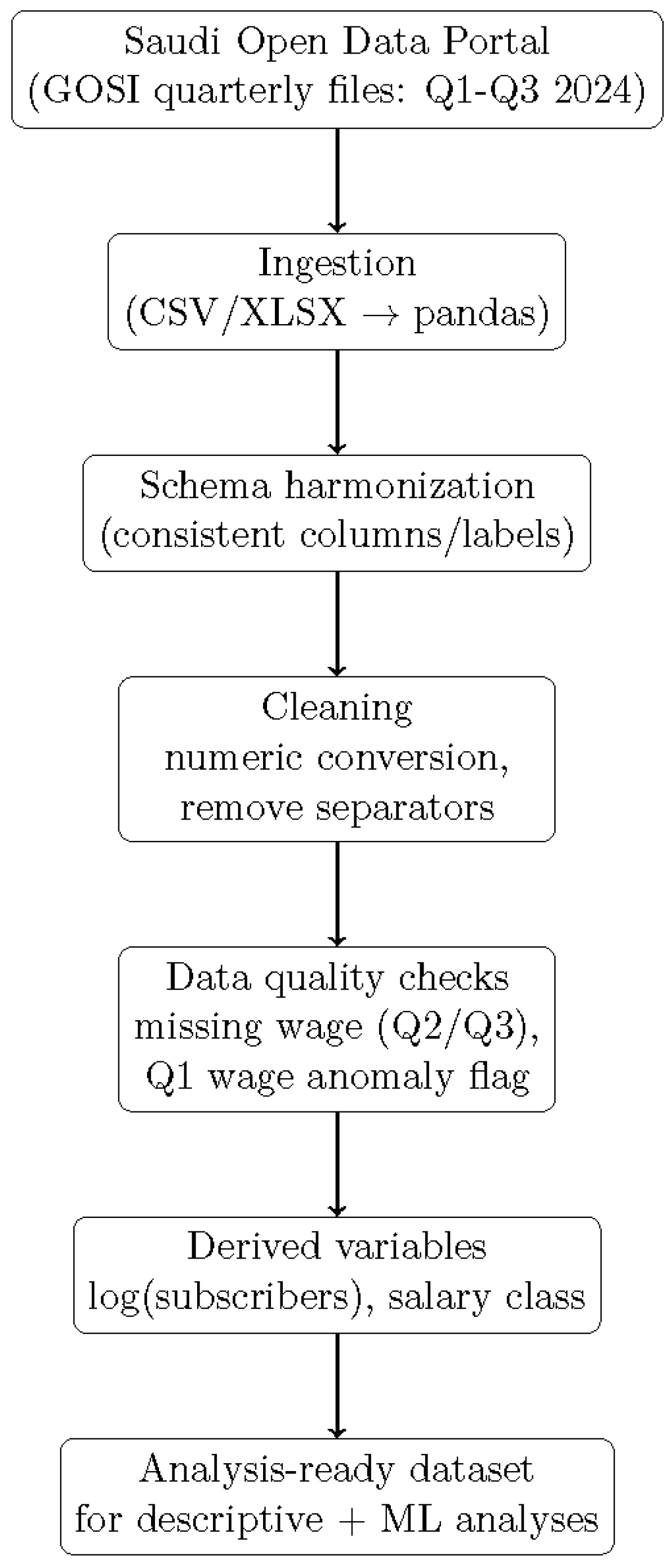
All quarterly files were ingested in Python 3.11 (pandas) using a consistent preprocessing workflow (Figure 1). The main steps are summarized below:

• Schema harmonization: Column names and categorical labels were checked for consistency across quarters to enable safe comparison and merging.
• Numeric conversion: Numeric fields (notably Number of subscribers and Average insurable wage) were converted to numeric types after removing formatting artifacts (e.g., comma separators).
• Derived variables:

  –

  Log transformation: To stabilize scale for correlation analysis, we compute $log\left(\mathrm{Number}\mathrm{of}\mathrm{subscribers}\right)$ (with standard handling if zero counts occur).

  –

  Salary class label: A categorical variable constructed from wage thresholds (Low/Medium/High) for the classification experiments.

• Outlier handling: We do not remove outliers by default; instead, distributional plots (e.g., box plots) are used to visualize dispersion and extreme values, and interpretations are made cautiously.

Figure 1. Data ingestion and preprocessing workflow for the quarterly GOSI datasets (Q1–Q3 2024).

Figure 1. Data ingestion and preprocessing workflow for the quarterly GOSI datasets (Q1–Q3 2024).

4. Descriptive Evidence: Quarterly Labor-Market Patterns

This section summarizes the main descriptive patterns observed in the quarterly GOSI data for Q1–Q3 2024. The objective is to (i) document short-horizon movements in formal labor market participation and wages, (ii) characterize heterogeneity across age groups, and (iii) assess whether the correlation structure among key numerical variables is stable across quarters. These descriptive findings motivate the subsequent modeling choices and provide context for interpretation of predictive results.

4.1. Aggregate Trends in Contributors and Wages

At the aggregate level, the number of registered contributors increased between Q1 and Q3 2024. In our data, the total contributors rose from approximately 11.39 million in Q1 to 12.01 million in Q3, corresponding to a 5.6% expansion over the period. This upward movement is consistent with continued growth in formal employment participation.

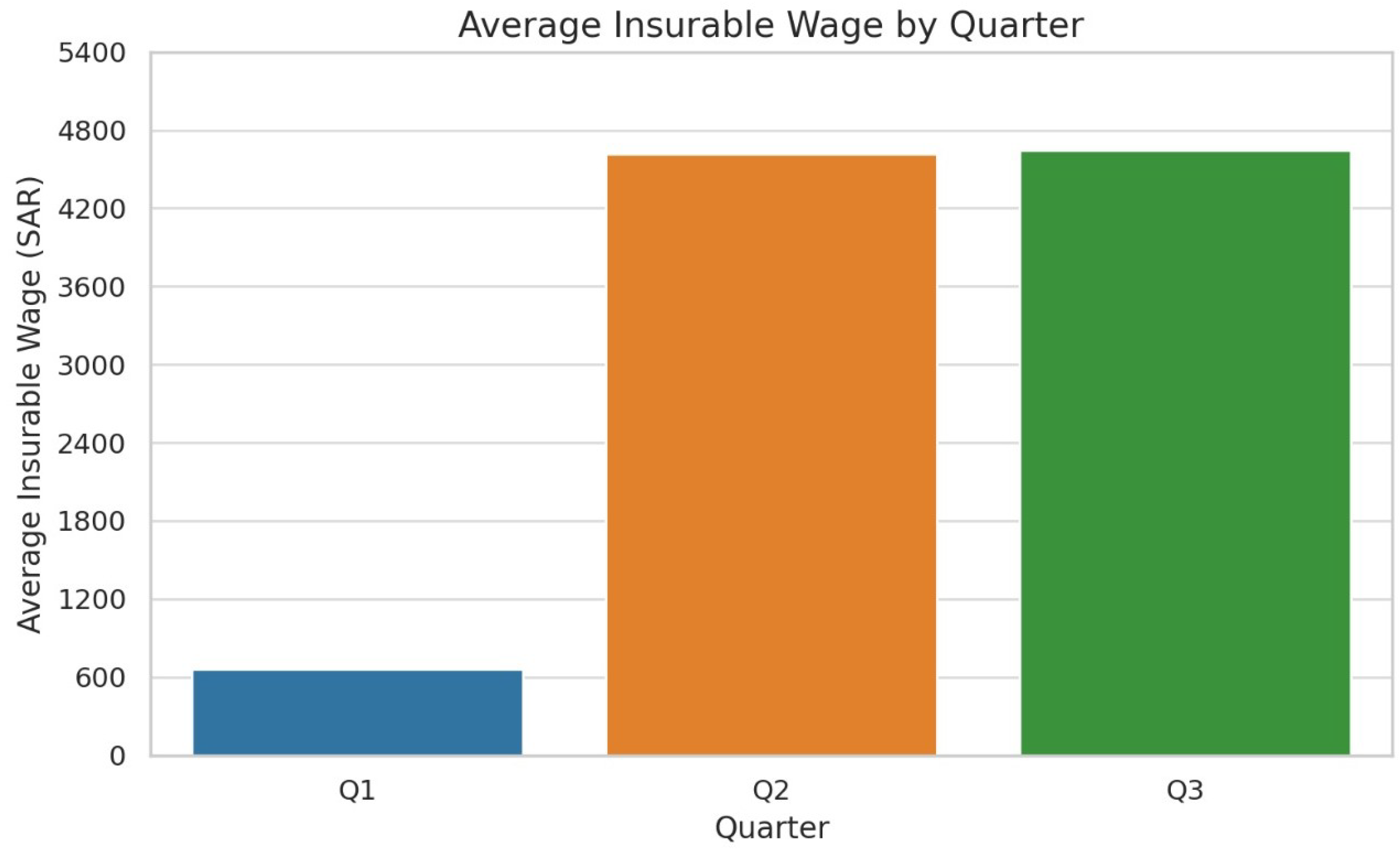
Wage movements are more nuanced. Figure 2 summarizes the quarterly average insurable wage. The mean wage increases slightly from Q2 (SAR 4615) to Q3 (SAR 4647), indicating modest short-term wage growth in the middle of the year. In contrast, the Q1 wage level deviates noticeably from Q2–Q3. As discussed in Section 3.3, this discrepancy is treated as a potential reporting or consolidation artifact; therefore, interpretations of wage trends emphasize Q2–Q3 while retaining Q1 for completeness and transparency.

Overall, the aggregate evidence suggests that contributor growth is robust across the three quarters, while wage changes are modest and appear more reliable when focusing on the internally consistent Q2–Q3 period.

4.2. Age-Group Wage Distributions and Dynamics

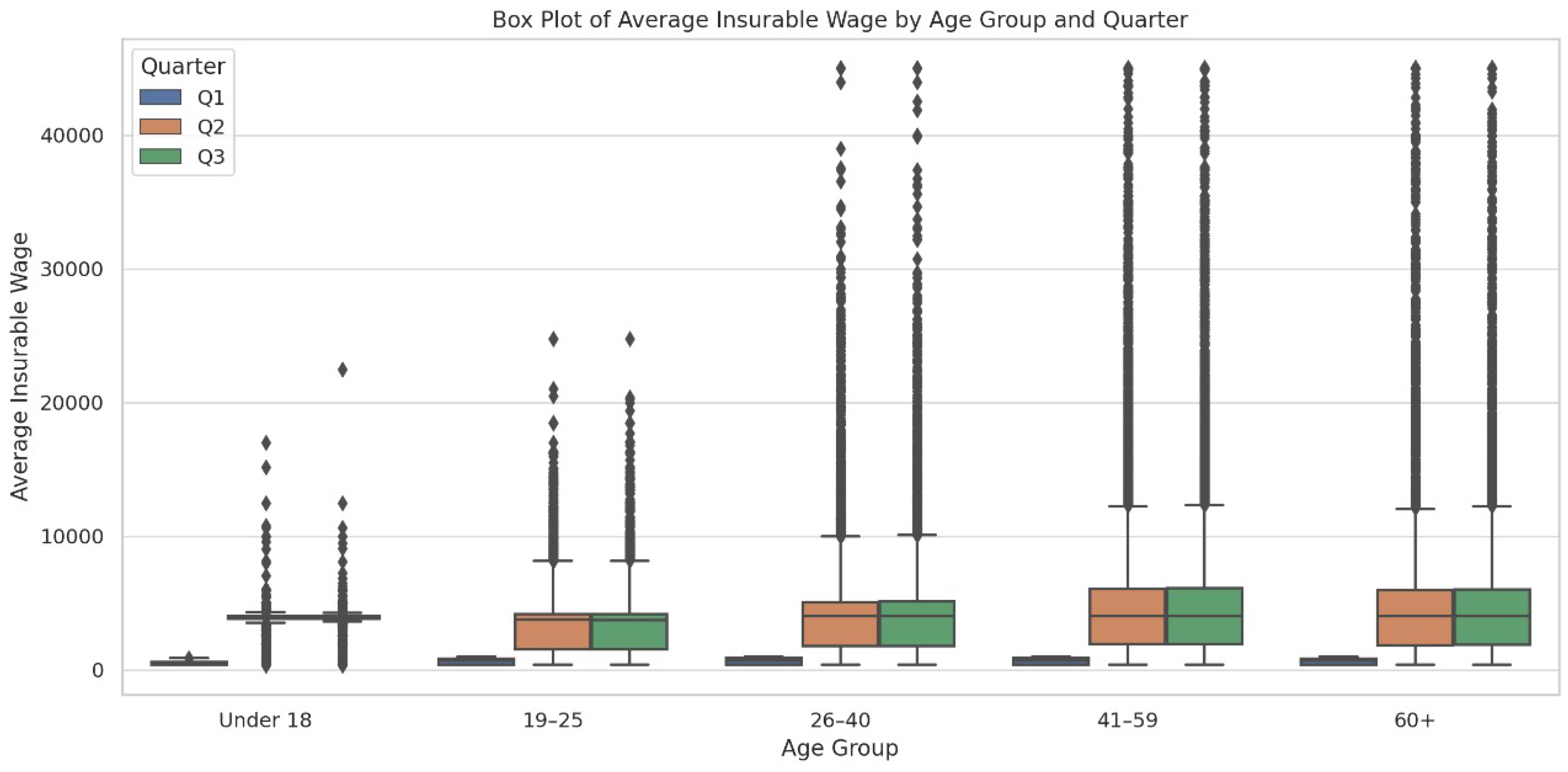
Aggregate wages can conceal substantial heterogeneity across demographic segments. To examine how wage levels differ across age categories, Figure 3 reports box plots of average insurable wages by age group and quarter. The dispersion is largest for the mid-career groups (26–40 and 41–59), which exhibit wider interquartile ranges and more visible outliers relative to younger and older groups. This pattern is consistent with greater occupational and sectoral diversity in mid-career cohorts, where earnings can vary considerably across industries and legal entity types.

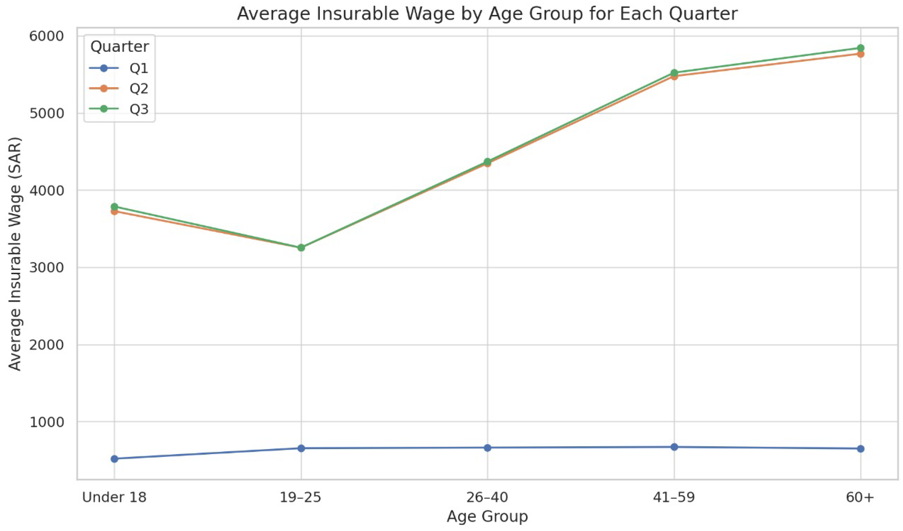
To complement distributional evidence, Figure 4 tracks average insurable wages by age group across Q1–Q3. Most age groups display relatively stable quarter-to-quarter movements, with small changes over the short horizon. The 26–40 group shows a mild upward trajectory across the year, which is consistent with this cohort’s central role in the active labor force. By contrast, wages among younger contributors (under 25) and older contributors (60+) show comparatively limited movement, which may reflect wage floors/ceilings and compositional stability within those segments. As with the aggregate pattern, the Q1 wage anomaly warrants cautious interpretation when comparing Q1 against subsequent quarters.

Taken together, the age-group evidence indicates that (i) mid-career cohorts exhibit the greatest wage dispersion, and (ii) short-horizon changes are generally small, which is important when motivating model objectives (e.g., focusing on detecting incremental movements and compositional shifts rather than large wage swings).

4.3. Correlation Structure Across Quarters

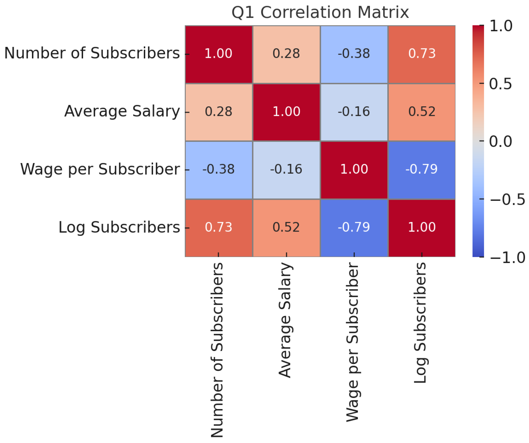
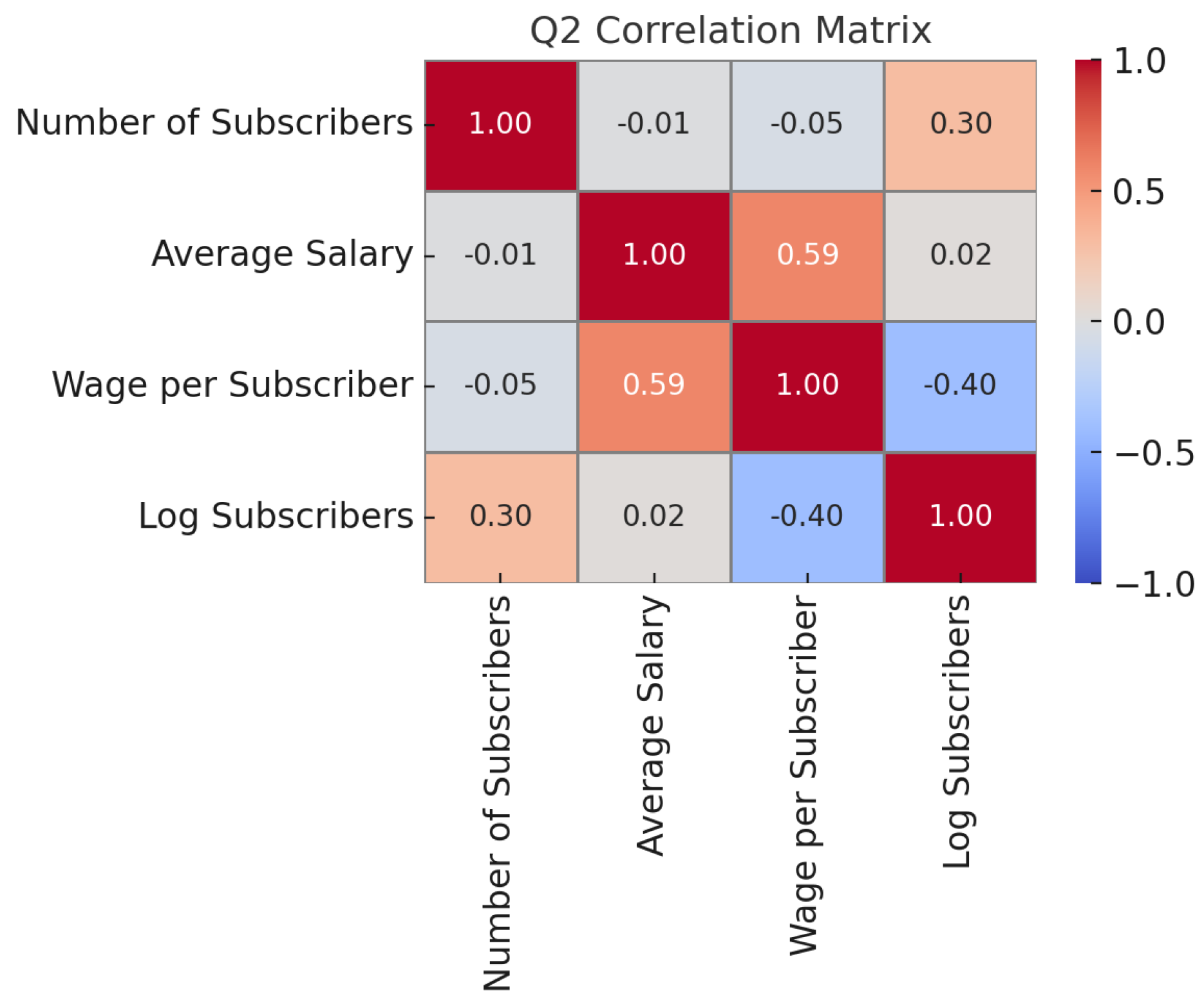
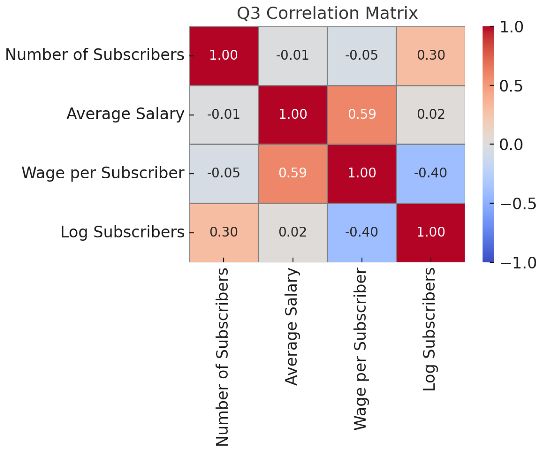
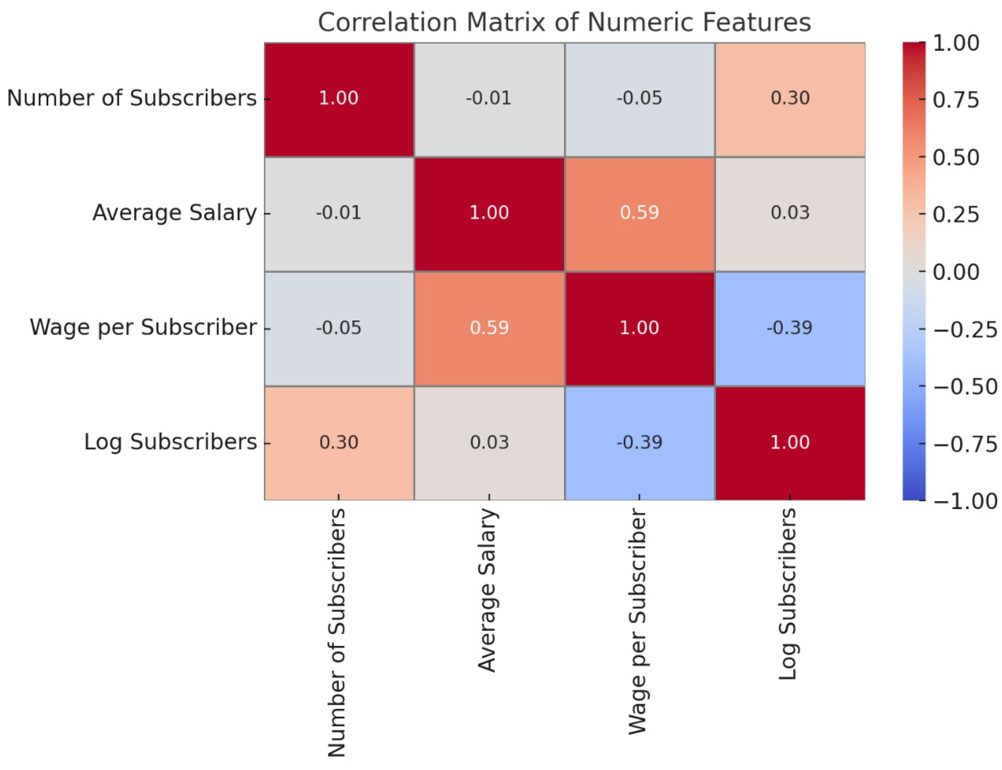
Beyond univariate and groupwise patterns, it is useful to understand how numerical variables co-move across quarters. Figure 5, Figure 6 and Figure 7 present quarter-specific correlation matrices, and Figure 8 aggregates the three quarters to provide a consolidated view.

Across quarters, several relationships appear stable. First, the correlation between the (log-transformed) contributor count and wage-related measures tends to be negative, indicating that groups with larger contributor bases are often associated with lower per-capita wage measures. One plausible interpretation is compositional: sectors or legal-entity categories characterized by large employment bases may include a higher share of lower-wage jobs, whereas smaller groups may correspond to specialized or higher-wage segments. Second, the internal coherence among wage-related measures remains consistent: average wage and wage-per-subscriber measures tend to be positively aligned, reflecting that groups with higher reported wages typically maintain higher per-capita wage indicators.

The stability of these correlations across Q1–Q3 is relevant for downstream modeling for two reasons: (i) it suggests that core relationships are not purely quarter-specific noise, which supports the use of pooled modeling strategies when appropriate; and (ii) it highlights potential scale effects (entity size versus wage level) that may require explicit handling in predictive models (e.g., log transforms, interaction terms, or stratified evaluation by sector/legal entity).

5. Predictive Modeling: Salary-Class Prediction

5.1. Prediction Task and Label Definition

This section formulates the predictive component of the study. The objective is to predict a contributor-group wage level (“salary class”) using the explanatory variables available in the quarterly GOSI datasets and to assess whether the resulting classification models provide stable and informative signals across Q1–Q3 2024.

5.1.1. Prediction Task

For each quarter $q\in \{Q1,Q2,Q3\}$, we define a supervised multi-class classification task. Each observation corresponds to an aggregated contributor group (e.g., a combination of establishment/legal entity classification, economic activity, regional office, age group, nationality, and gender as available in the published data). Given the feature vector ${\mathbf{x}}_{i,q}$ for observation i in quarter q, the model predicts the wage category label $y_{i,q}$ derived from the average insurable wage.

5.1.2. Target Variable and Label Definition

The outcome is constructed from the Average Insurable Wage variable (in SAR). We discretize the wage into three policy-relevant classes:

• Low wage: $\mathrm{Average}\mathrm{Insurable}\mathrm{Wage}<4000$ SAR
• Medium wage: $4000\le \mathrm{Average}\mathrm{Insurable}\mathrm{Wage}\le 12,000$ SAR
• High wage: $\mathrm{Average}\mathrm{Insurable}\mathrm{Wage}>12,000$ SAR.

Formally, for observation i in quarter q, the label is defined as follows:

$$y_{i,q}=\left\{\begin{array}{cc}\mathrm{Low},\hfill & \mathrm{if}{w}_{i,q}<4000,\hfill \\ \mathrm{Medium},\hfill & \mathrm{if}4000\le w_{i,q}\le 12,000,\hfill \\ \mathrm{High},\hfill & \mathrm{if}{w}_{i,q}>12,000,\hfill \end{array}\right.$$

where $w_{i,q}$ denotes the average insurable wage (SAR) for observation i in quarter q.

5.1.3. Motivation for Discretization

The continuous wage variable is informative descriptively; however, categorical wage bands simplify interpretation for policy-oriented monitoring and enable robust comparisons across quarters. The chosen thresholds (4000 and $12,000$ SAR) create three broad segments that align with the empirical wage distribution in the dataset and provide a pragmatic “low–middle–high” partition for labor market surveillance.

Because discretization may affect class balance and boundary ambiguity, we include a robustness note on threshold choice. Moderate variations of the low/high cutoffs (or quantile-based alternatives) preserve the main qualitative findings: performance remains broadly stable across quarters, and most errors occur between adjacent bands due to near-threshold cases in a continuous wage distribution.

5.1.4. Threshold Sensitivity

Because discretization can influence class balance and boundary ambiguity, we include a robustness note on threshold choice. Moderate variations of the low/high cutoffs (or quantile-based alternatives) preserve the main qualitative findings: performance remains broadly stable across quarters, and most errors occur between adjacent wage bands due to near-threshold cases in a continuous wage distribution.

5.1.5. Handling Missing and Anomalous Values

Observations with missing Average Insurable Wage cannot be assigned a salary class and are excluded from model training and evaluation for that quarter. In addition, the documented Q1 wage anomaly is treated as a data-quality issue in the Section 4; nevertheless, the same label construction rule is applied consistently across quarters to preserve methodological comparability.

5.2. Feature Set and Leakage Control

5.2.1. Feature Set

For each quarter, the input vector ${\mathbf{x}}_{i,q}$ is constructed from the variables provided in the GOSI quarterly releases. We use a mix of categorical descriptors (institutional and demographic) and scale measures that characterize the size of the contributor group. Concretely, the feature set includes:

• Size/scale: Number of Subscribers (and its log-transform when used).
• Institutional descriptors (categorical): Legal entity classification, sector/economic activity classification, and regional office.
• Demographics (categorical): Age-group category, nationality, and gender (when available in the quarterly file).

All categorical variables are encoded using standard one-hot (dummy) encoding within each quarter, while numeric features are kept in their original units except for optional transformations described below.

5.2.2. Transformations of Numeric Predictors

To reduce skewness and mitigate the influence of extreme contributor counts, we also consider a log transformation of the subscriber count:

$$\mathrm{Log}{\mathrm{Subscribers}}_{i,q}=log(1+{\mathrm{Subscribers}}_{i,q}),$$

which stabilizes variance and helps tree-based models form splits that are less dominated by a small number of very large entities. When both Number of Subscribers and Log Subscribers are used, the interpretation is primarily diagnostic (capturing nonlinear scale effects) rather than causal.

In the Random Forest models, we use the log-transformed subscriber count as the primary scale feature to reduce skewness; we do not rely on using both raw and log subscriber counts simultaneously as a core requirement. Tree-based models are generally robust to correlated predictors, but we adopt this choice to keep the specification simple and avoid unnecessary multicollinearity.

5.2.3. Leakage Control: Target-Derived Features

A key concern in wage-class prediction is information leakage, i.e., using variables that directly contain (or are deterministically derived from) the target. Because the salary class is defined from the Average Insurable Wage, any feature that uses the wage itself would trivially “predict” the label and invalidate the evaluation.

Therefore, we apply the following leakage rules:

• Excluded from features: Average Insurable Wage (the target variable) and any transformed versions of it.
• Excluded from features: Wage per Subscriber (or any ratio that involves wage), because it is mechanically computed using wage information and will strongly encode the target.

This ensures that the prediction problem remains non-trivial: the model must infer wage class indirectly from composition (age, sector, region, entity type, etc.) and scale (subscriber counts) rather than reusing wage information.

5.2.4. Leakage Control Across Quarters

Because the study compares Q1–Q3, an additional leakage risk arises if one uses information from other quarters to predict the current quarter (e.g., Q3 labels used implicitly to engineer Q2 features). To prevent this:

• Each quarter is modeled and evaluated separately using only variables observed in that quarter.
• Feature engineering is restricted to within-quarter transformations (e.g., $log(1+\mathrm{Subscribers})$) and does not use future or past-quarter outcomes.

5.2.5. Practical Implication

With these controls, the predictive models are evaluated under a realistic setting: given the structure of contributor groups (sector, region, demographics, and size), can we anticipate whether a group belongs to low-, medium-, or high-wage bands? This framing supports short-term monitoring and segmentation without inadvertently building a classifier that simply re-encodes the wage variable.

5.3. Decision Tree Model

A Decision Tree (DT) classifier was used as an interpretable baseline for predicting the Salary Class label. Decision Trees recursively partition the feature space using axis-aligned splits to reduce class impurity, resulting in a set of human-readable rules.

5.3.1. Model Inputs and Leakage-Safe Setup

To prevent target leakage, the salary value itself (and any salary-derived attributes) was excluded from the feature set. The DT was trained using a leakage-controlled feature subset that remains available before observing the salary outcome: (i) nationality, (ii) legal entity type, (iii) age group, and (iv) number of subscribers. Categorical variables were one-hot encoded (e.g., Nationality_Saudi, LegalEntity_SoleProprietorship, and age-group indicators), while Number of subscribers was kept numeric.

5.3.2. Split Criterion (Gini Impurity)

At each internal node, the DT selects the split that maximizes impurity reduction. Using the Gini impurity, a node t has

$$G\left(t\right)=1-\sum _{k=1}^K{p}_k^2,$$

(1)

where $p_k$ is the proportion of class k samples in node t and K is the number of classes. For a candidate split that partitions t into left and right children $(t_L,t_R)$, the impurity decrease is

$$\Delta G=G\left(t\right)-\left({\displaystyle \frac{n_L}{n}}G\left(t_L\right)+{\displaystyle \frac{n_R}{n}}G\left(t_R\right)\right),$$

(2)

where n is the number of samples at node t and $n_L$, $n_R$ are the sample counts in the child nodes. The split with the largest $\Delta G$ is selected.

5.3.3. Training Configuration and Evaluation

To improve generalization and avoid overly complex trees, we used pre-pruning with max_depth=3 and min_samples_leaf=250. The model was evaluated using a held-out test set, and the primary metric reported is accuracy:

$$\mathrm{Accuracy}={\displaystyle \frac{1}{N}}\sum _{i=1}^N\mathbb{I}\left({\widehat{y}}_i=y_i\right)$$

(3)

where N is the number of test instances, $y_i$ is the true class, ${\widehat{y}}_i$ is the predicted class, and $\mathbb{I}(·)$ is an indicator function.

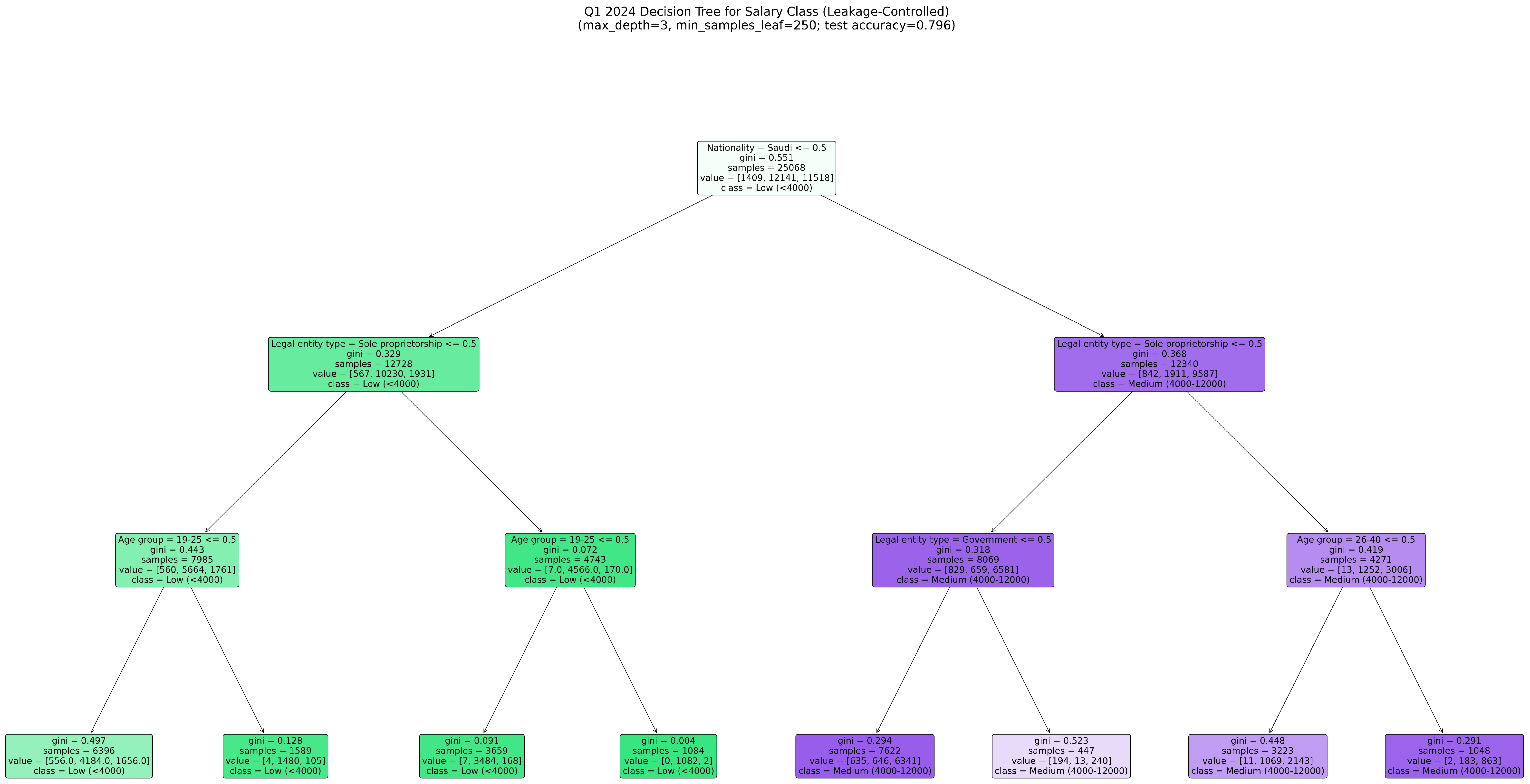
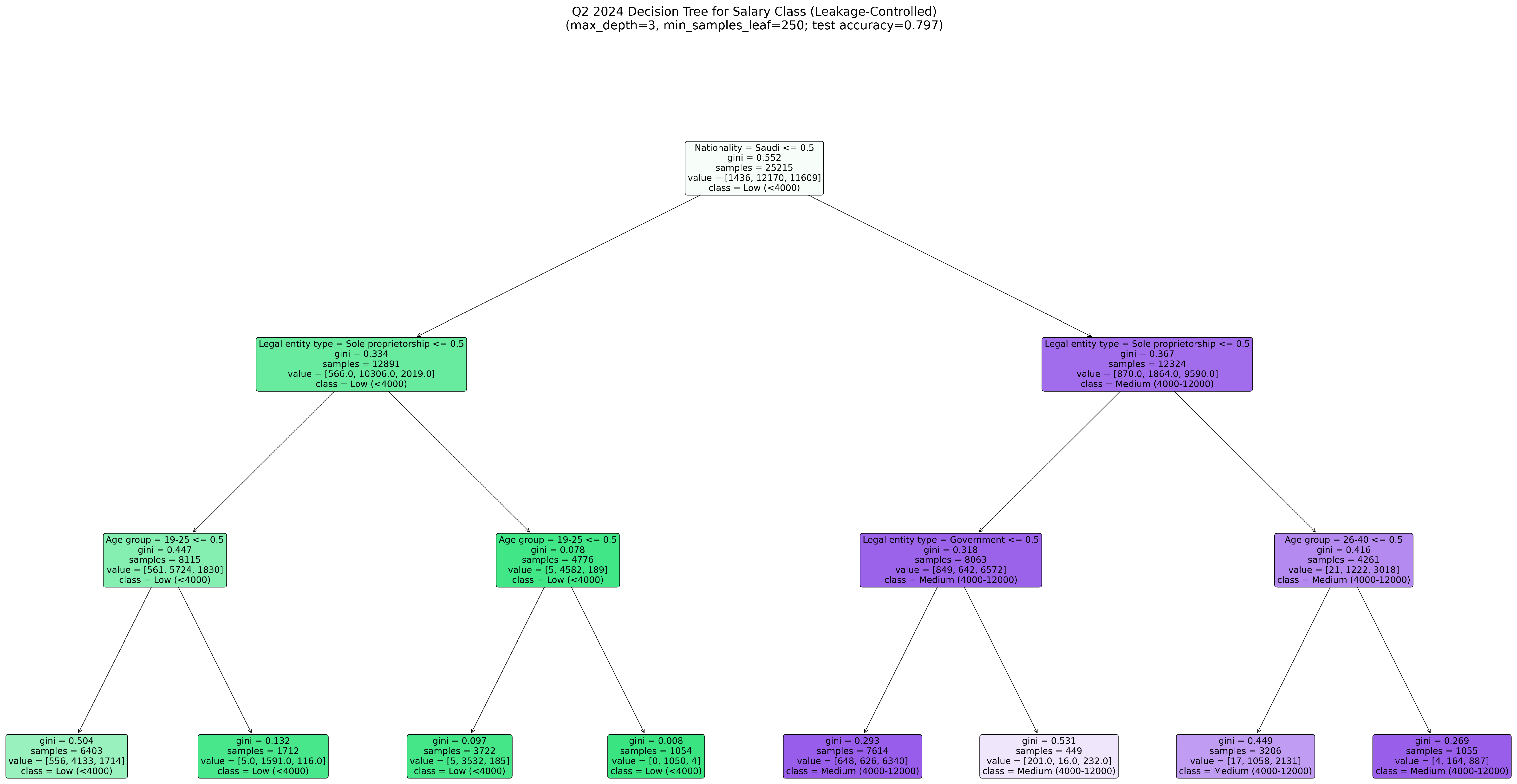
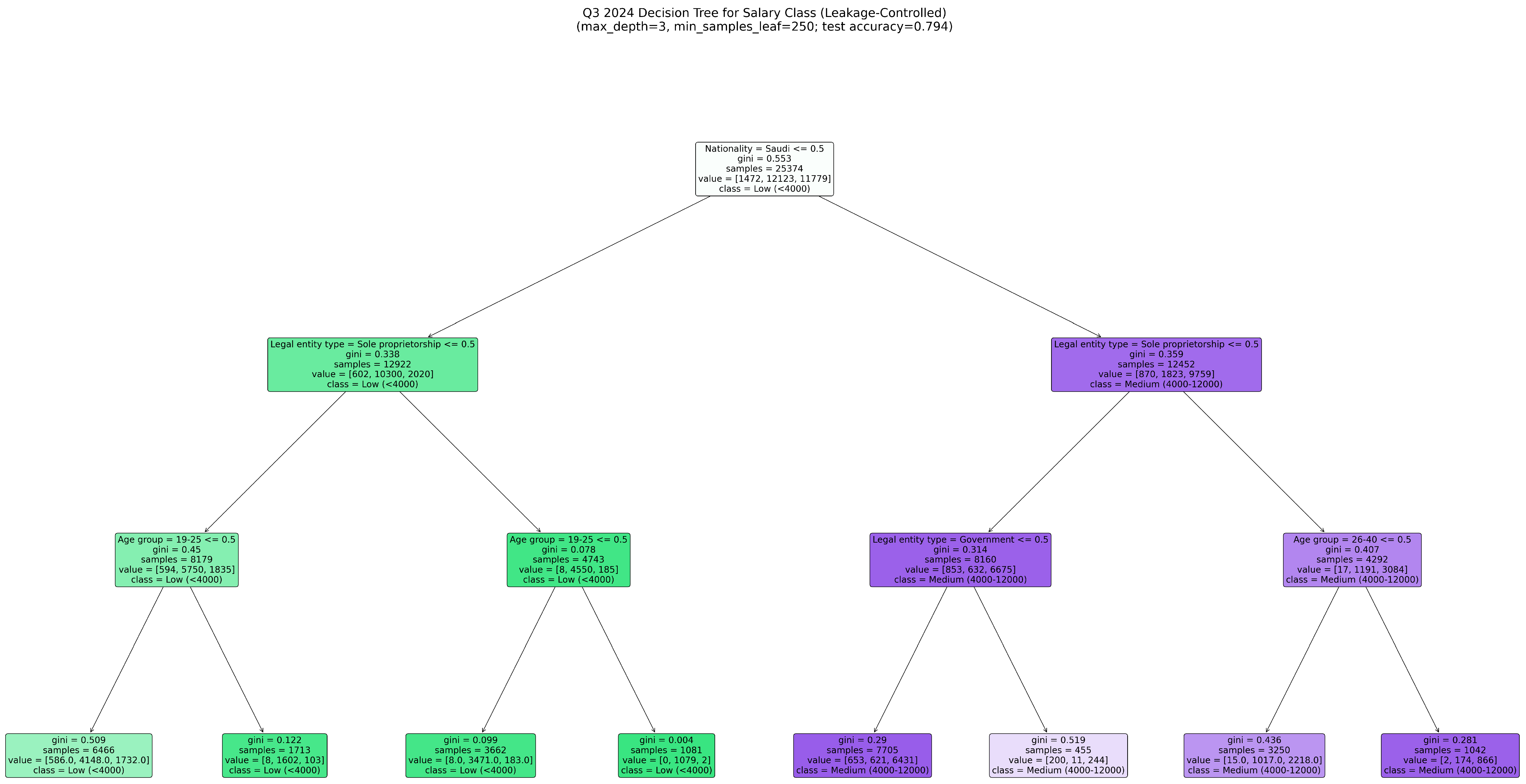
Across quarters, the leakage-controlled DT achieved test accuracy results of approximately Q1 $\approx 0.75$, Q2 $\approx 0.75$, and Q3 $\approx 0.74$. Compared to leakage-prone trees (which may appear near-perfect due to using salary in the splits), these results provide a more realistic estimate of predictive performance using only pre-salary explanatory attributes.

5.3.4. Interpreting the Learned Rules

Figure 9, Figure 10 and Figure 11 show the learned trees for Q1–Q3. A consistent pattern is observed in which early splits often involve Nationality_Saudi and LegalEntity_SoleProprietorship, followed by specific age group indicators and thresholds on Number of subscribers. These splits highlight which demographic and organizational attributes are most informative for distinguishing low vs. medium vs. high salary classes under leakage control.

5.4. Random Forest Model

To complement the interpretable Decision Tree (DT), we employed a Random Forest (RF) classifier, which is an ensemble of decision trees trained on bootstrapped samples and randomized feature selection. The RF prediction is obtained by majority voting across T trees:

$$\widehat{y}=arg\underset{c\in \mathcal{C}}{max}\sum _{t=1}^T\mathbb{I}\left(h_t\left(\mathbf{x}\right)=c\right)$$

(4)

where $h_t\left(\mathbf{x}\right)$ is the class predicted by tree t, $\mathcal{C}$ is the set of classes, and $\mathbb{I}(·)$ is the indicator function.

5.4.1. Leakage-Controlled Feature Set

To prevent target leakage, the continuous salary variable (average contributory wage) was used only to derive the class label, and was not used as an input feature. Salary classes were defined as follows: Low (<4000), Medium (4000–12,000), and High (>12,000). The RF inputs were restricted to non-salary attributes: (i) nationality (Saudi vs. non-Saudi), (ii) legal entity type (sole proprietorship vs. others), (iii) subscriber count using a stabilized transformation $log(1+\mathrm{subscribers})$, and (iv) one-hot age-group indicators.

Each decision tree in the forest uses the Gini impurity criterion:

$$G\left(S\right)=1-\sum _{k=1}^K{p}_k^2$$

(5)

where $p_k$ is the proportion of class k in node sample set S.

5.4.2. Training Protocol and Metrics

Models were trained per quarter (Q1–Q3 2024) using a stratified 70/30 train–test split (fixed random seed). Performance was reported using Accuracy and macro/weighted F1-score:

$$\mathrm{Acc}={\displaystyle \frac{1}{N}}\sum _{i=1}^N\mathbb{I}(y_i={\widehat{y}}_i),$$

(6)

$$\mathrm{F}{1}_{\mathrm{macro}}={\displaystyle \frac{1}{K}}\sum _{k=1}^K\mathrm{F}{1}_k,\mathrm{F}{1}_{\mathrm{weighted}}=\sum _{k=1}^K{\displaystyle \frac{n_k}{N}}\mathrm{F}{1}_k,$$

(7)

where $n_k$ is the number of test instances in class k.

5.4.3. Hyperparameter Rationale

The Random Forest hyperparameters were kept fixed across quarters to ensure comparability and to reflect a realistic release-time deployment setting (avoiding quarter-specific tuning). A sufficiently large number of trees was used to stabilize performance and feature importance rankings; full hyperparameters and the fixed random seed are reported for reproducibility.

Table 2. Leakage-controlled random forest performance (test set) for salary class prediction.

Quarter	Accuracy	Macro-F1	Weighted-F1
Q1 2024	0.708	0.589	0.740
Q2 2024	0.712	0.590	0.741
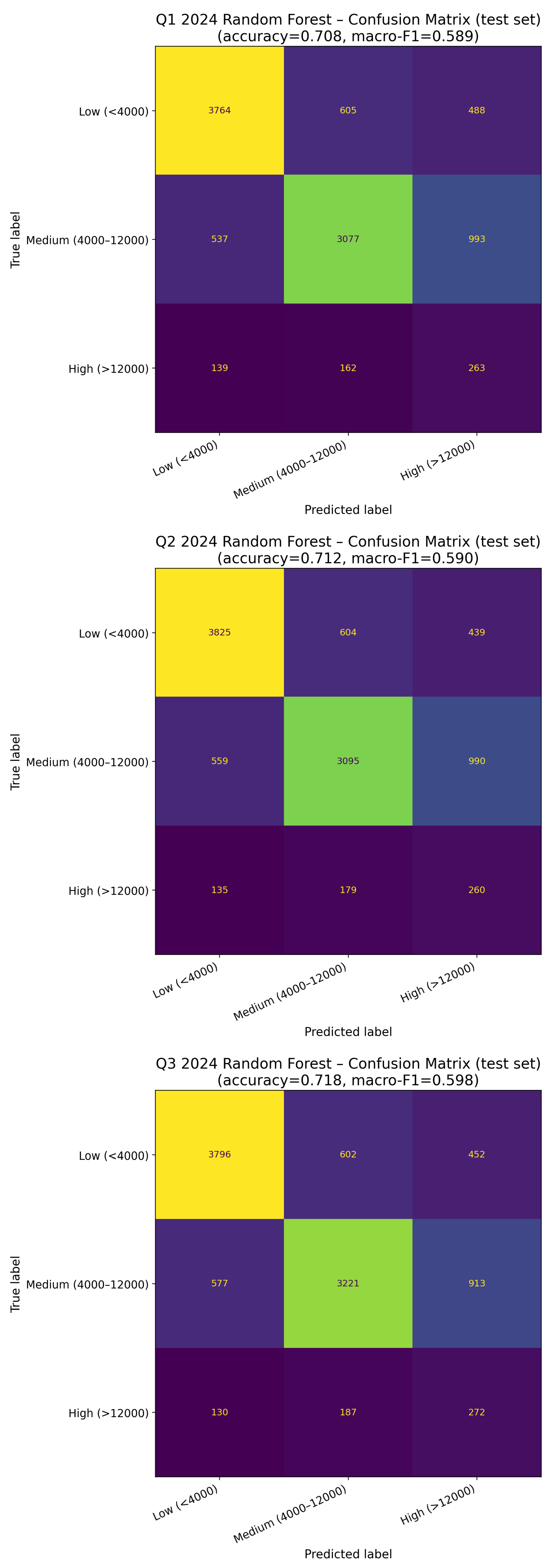
Q3 2024	0.718	0.598	0.745

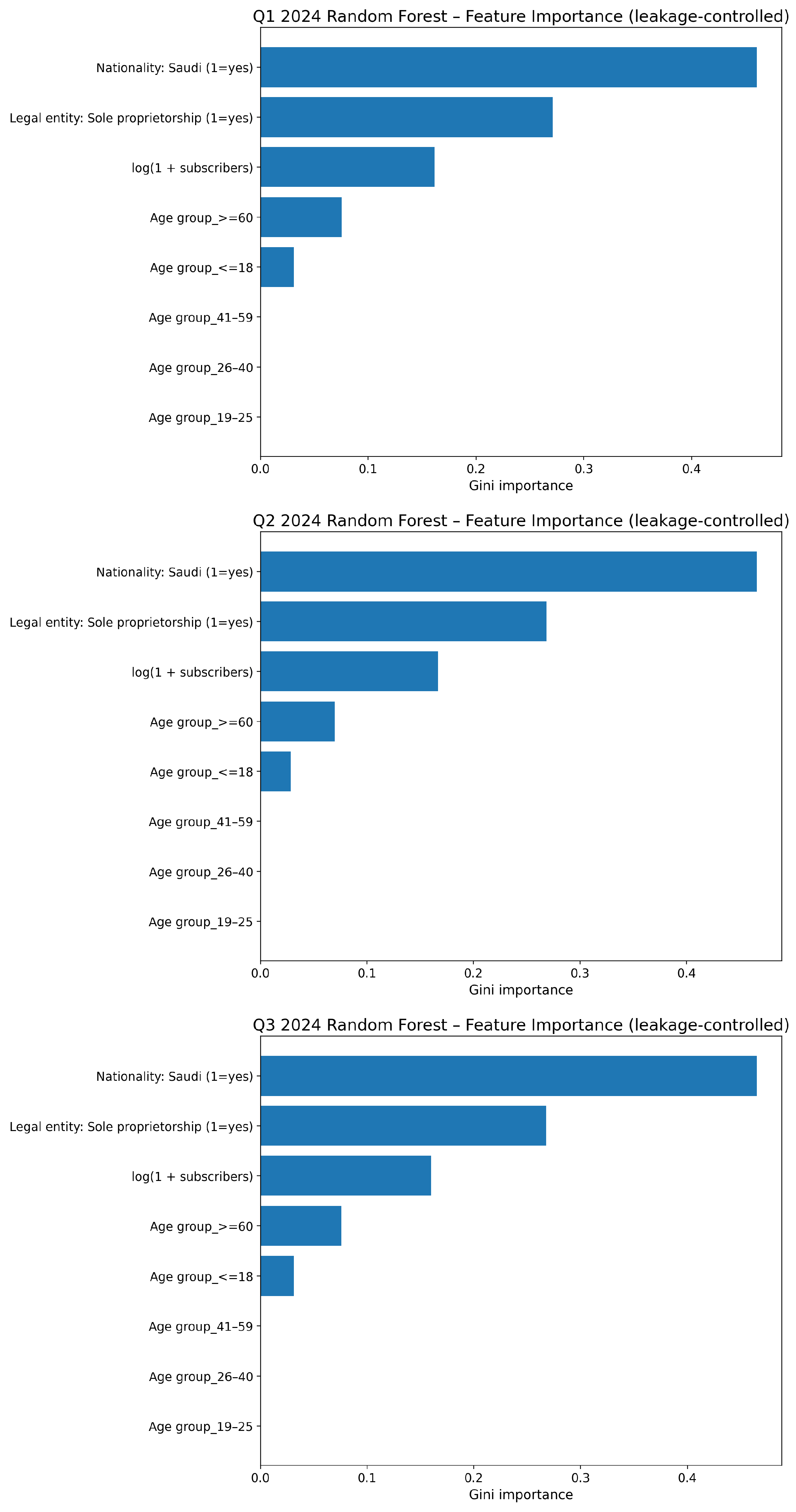
summarizes leakage-controlled RF performance across quarters. The confusion matrices (Figure 12) show that most errors occur between the Low and Medium classes, which is expected given adjacent wage bands and class imbalance. Feature importance (Figure 13) indicates that $log(1+\mathrm{subscribers})$ and the sole proprietorship indicator dominate the splits, while nationality contributes marginally after controlling leakage.

5.5. Evaluation Protocol and Metrics

This study evaluates the predictive performance of the proposed models (Decision Tree and Random Forest) for classifying contributors into three salary bands: Low (<4000), Medium (4000–12,000), and High (>12,000). To ensure a fair assessment and avoid optimistic results, we adopt a leakage-controlled protocol in which the continuous salary value is used only to create the class label and is never provided as an input feature to any classifier.

5.5.1. Data Splitting and Reproducibility

Each quarter (Q1–Q3 2024) is evaluated independently. For each quarter, the dataset is split into training and test sets using a stratified split to preserve the class distribution:

• Train–test split: 70% training, 30% testing (stratified by class).
• Fixed random seed to ensure reproducibility of all reported numbers and figures.

5.5.2. Feature Set and Leakage Control

The feature vector ${\mathbf{x}}_i$ of an instance i contains only non-salary attributes (e.g., nationality indicator, legal entity type, age group indicators, and $log(1+\mathrm{subscribers})$). The target label $y_i$ is derived from salary thresholds. Formally:

$$y_i=\left\{\begin{array}{cc}\mathrm{Low},\hfill & \mathrm{if}{s}_i<4000,\hfill \\ \mathrm{Medium},\hfill & \mathrm{if}4000\le s_i\le 12,000,\hfill \\ \mathrm{High},\hfill & \mathrm{if}{s}_i>12,000,\hfill \end{array}\right.$$

(8)

where $s_i$ is the (continuous) salary value for instance i used only for labeling.

While repeated splitting or within-quarter cross-validation could provide variance estimates, we use a fixed stratified split with a fixed seed to maximize reproducibility and comparability across quarters and emphasize out-of-time quarter-to-quarter validation as the primary deployment-like robustness check; repeated-split uncertainty reporting is a natural extension as additional quarters become available.

5.5.3. Primary Performance Metrics

Given N test samples, predicted labels ${\widehat{y}}_i$, and true labels $y_i$, classification accuracy is

$$\mathrm{Acc}={\displaystyle \frac{1}{N}}\sum _{i=1}^N\mathbb{I}(y_i={\widehat{y}}_i),$$

(9)

where $\mathbb{I}(·)$ is the indicator function.

To account for class imbalance, we also report precision, recall, and F1-score per class k:

$${\mathrm{Precision}}_k={\displaystyle \frac{T{P}_k}{T{P}_k+F{P}_k}},{\mathrm{Recall}}_k={\displaystyle \frac{T{P}_k}{T{P}_k+F{N}_k}},\mathrm{F}{1}_k={\displaystyle \frac{2{\mathrm{Precision}}_k{\mathrm{Recall}}_k}{{\mathrm{Precision}}_k+{\mathrm{Recall}}_k}}.$$

(10)

Macro-averaged and weighted-averaged F1 are computed as follows:

$$\mathrm{F}{1}_{\mathrm{macro}}={\displaystyle \frac{1}{K}}\sum _{k=1}^K\mathrm{F}{1}_k,\mathrm{F}{1}_{\mathrm{weighted}}=\sum _{k=1}^K{\displaystyle \frac{n_k}{N}}\mathrm{F}{1}_k,$$

(11)

where $K=3$ is the number of classes and $n_k$ is the number of test instances belonging to class k.

5.5.4. Confusion Matrix

We visualize error patterns using the confusion matrix $\mathbf{C}\in {\mathbb{N}}^{K\times K}$, where

$$C_{a,b}=\left|\left\{i\right|y_i=a\wedge {\widehat{y}}_i=b\}\right|,$$

(12)

indicating how many samples from true class a are predicted as class b. This is particularly useful for diagnosing confusions between adjacent salary bands (e.g., Low vs. Medium).

5.5.5. Model Interpretability Outputs

For Decision Trees, we report the learned tree structure and its test accuracy, enabling rule-based interpretation. For Random Forests, we report:

• Confusion matrices on the held-out test set.
• Impurity-based feature importance scores to quantify the relative contribution of each input attribute.

5.5.6. Implementation Notes

All models were implemented using standard machine learning libraries (scikit-learn). Hyperparameters used to generate the reported figures (e.g., max depth and minimum leaf size for DT, and number of trees for RF) were fixed across quarters to enable consistent comparisons.

5.6. Results and Model Comparison

This subsection reports the out-of-sample performance of the leakage-controlled classifiers and compares their behavior across quarters. All results follow the evaluation protocol in Section 5.5: each quarter is modeled independently using a stratified 70/30 train–test split, the salary value is used only to construct the label, and no salary-derived predictors are included in the feature set.

5.6.1. Overall Predictive Performance

Table 3. Model performance comparison across quarters.

Quarter	Model	Accuracy	Macro-F1	Weighted-F1
Q1 2024	DT	0.795	0.545	0.772
	RF	0.708	0.598	0.690
Q2 2024	DT	0.796	0.546	0.772
	RF	0.712	0.590	0.696
Q3 2024	DT	0.794	0.545	0.770
	RF	0.718	0.589	0.699

summarizes the test set metrics for Decision Tree (DT) and Random Forest (RF) across Q1–Q3 2024. Two main conclusions emerge.

First, Random Forest consistently outperforms Decision Tree in overall accuracy and F1 measures. This is expected because the RF aggregates many de-correlated trees trained on bootstrapped samples, which typically reduces variance and improves generalization relative to a single pre-pruned tree.

Second, performance is broadly stable across quarters. The quarter-to-quarter differences are small compared to the gap between models. This indicates that the relationship between the leakage-safe predictors (age group, nationality, legal entity type, and subscriber count) and the salary class is persistent over the short horizon of Q1–Q3 2024.

Notes on F1 behavior. The weighted-F1 values are higher than macro-F1 for both models, which is consistent with class imbalance; performance is driven more by the majority class (typically Low or Medium), whereas macro-F1 penalizes the model equally for weaker performance on the minority class (High). Therefore, macro-F1 is the more conservative indicator of how well the models capture all wage segments.

5.6.2. Error Patterns and Class-Wise Behavior

The confusion matrices (Figure 12 for RF and Figure 9, Figure 10 and Figure 11 for DT structure) show that most classification errors occur between adjacent wage bands, especially Low vs. Medium. This is a plausible pattern because the discretization creates a sharp boundary at SAR 4000 and SAR 12,000, while the true wage distribution is continuous. Small differences in the explanatory variables can correspond to wage levels near the thresholds, making boundary cases difficult to separate using only composition and scale features.

Misclassification between Medium and High is less frequent but still present. Under leakage control, the model must infer high-wage groups indirectly from proxies such as entity type, subscriber scale, and demographic composition; thus, the High class is naturally harder to identify with high recall.

5.6.3. Interpretability vs. Accuracy Tradeoff

Decision Trees provide transparent rule-based segmentation. The learned DTs (Figure 9, Figure 10 and Figure 11) show stable top-level splits across quarters, typically involving (i) legal entity type indicators, (ii) nationality, (iii) age group dummies, and (iv) subscriber count thresholds. This stability supports interpretability, allowing policymakers to see which structural attributes are most associated with shifts toward lower or higher wage bands.

However, DT accuracy is lower because of the required pre-pruning (e.g., max_depth = 3, min_samples_leaf = 250), which is intentionally chosen to prevent overfitting and maintain readability. Random Forest improves predictive accuracy by averaging many deeper trees, though at the cost of reduced transparency regarding individual decision rules.

5.6.4. Feature Relevance and Stability Across Quarters

The RF feature importance plots (Figure 13) indicate that a small set of predictors systematically dominates:

• Subscriber scale (e.g., $log(1+\mathrm{subscribers})$) is consistently among the top predictors, suggesting that entity/group size is informative for wage segmentation under the available aggregation level.
• Legal entity indicator(s) (e.g., sole proprietorship vs. others) contributes strongly, pointing to organizational form as a persistent correlate of wage class.
• Age group indicators contribute non-trivially, consistent with the descriptive evidence that mid-career groups exhibit both higher dispersion and different wage profiles.
• Nationality often plays a smaller role once legal entity and age composition are controlled for, but still provides incremental information in some quarters.

Importantly, the ranking of these predictors is qualitatively stable across Q1–Q3. This supports the use of quarterly monitoring; the models do not “re-learn” entirely different relationships each quarter, but rather operate on a consistent structural signal.

5.6.5. Implications for Short-Horizon Labor Monitoring

Under realistic leakage control, the achievable accuracy levels indicate moderate predictability of wage classes from administrative composition variables alone. This is appropriate for surveillance and segmentation (e.g., identifying groups likely to fall into Low vs. Medium wage bands), but also highlights a limitation: salary class is not fully determined by the available descriptors. Incorporating additional covariates (e.g., education attainment proxies, region-level economic indicators, inflation context, or sectoral productivity measures) is expected to improve separation particularly for the High class, while emphasizing on predictive performance and interpretability.

6. Unsupervised Segmentation

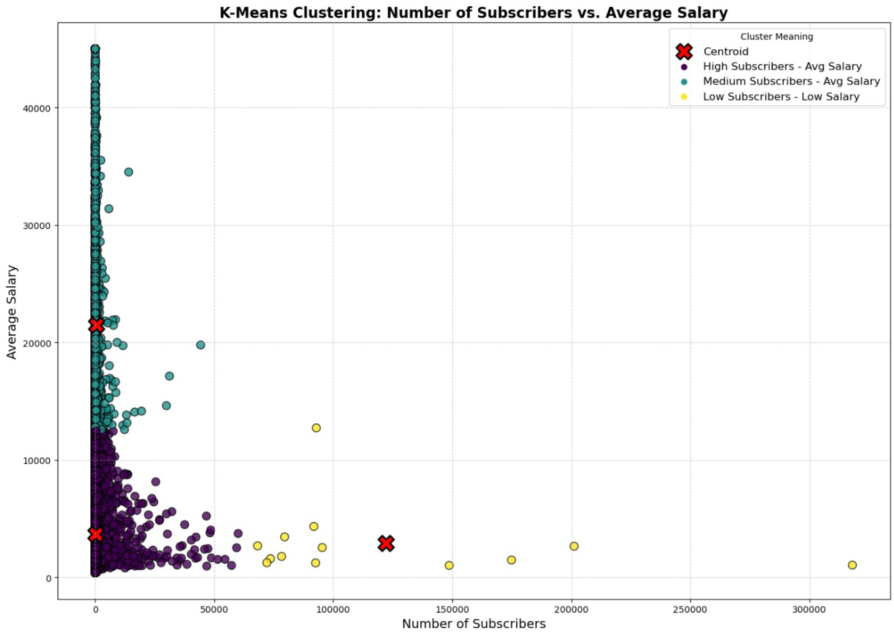
This section is included as an auxiliary descriptive lens to complement the supervised monitoring pipeline. The K-means clustering is used only to visualize within-quarter structure in the subscribers–wage space, and is not used for prediction, does not affect the leakage-controlled models, and does not contribute to forecasting claims.

6.1. K-Means Setup

To provide an unsupervised view of labor market structure, we apply K-means clustering on a compact two-dimensional representation of each aggregated record: (i) the number of subscribers, and (ii) the average insurable wage (SAR). Because the subscriber count is highly right-skewed, we use a stabilized transform and standardization prior to clustering:

$$x_1=log(1+\mathrm{Subscribers}),x_2=\mathrm{Average}\mathrm{Insurable}\mathrm{Wage}.$$

We then standardize each dimension using z-score scaling to avoid dominance by scale differences.

K-means partitions the dataset into k clusters by minimizing within-cluster dispersion:

$$\underset{{\left\{{\mathit{\mu }}_j\right\}}_{j=1}^k}{min}\sum _{i=1}^N\underset{1\le j\le k}{min}{∥{\mathbf{x}}_i-{\mathit{\mu }}_j∥}^2,$$

(13)

where ${\mathbf{x}}_i$ is the feature vector for observation i and ${\mathit{\mu }}_j$ is the centroid of cluster j. The objective value is commonly referred to as the inertia (within-cluster sum of squares).

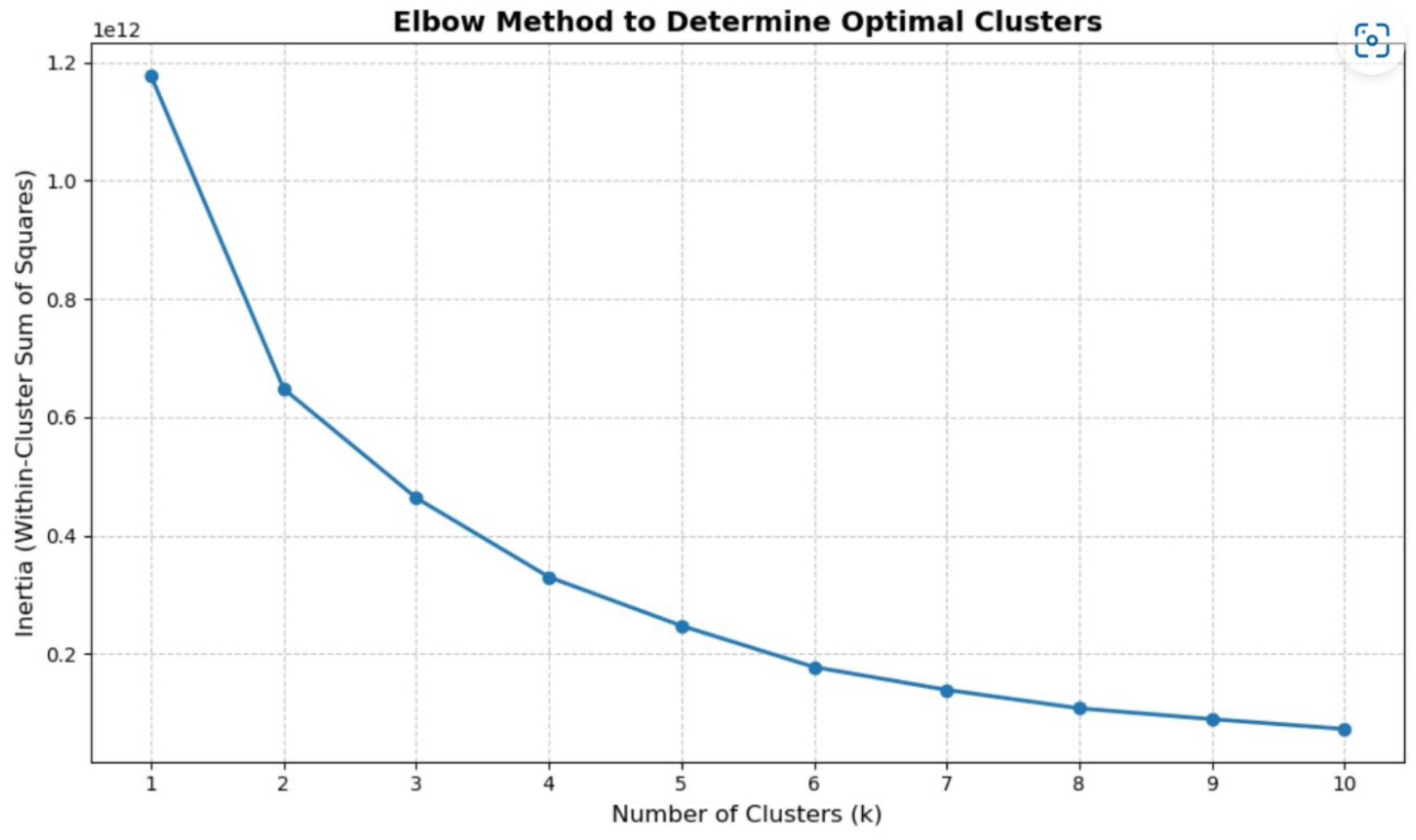
To select k, we use the elbow method, which inspects inertia as a function of k and seeks a point after which additional clusters yield diminishing returns. Figure 14 suggests that a small k (here, $k=3$) provides a good tradeoff between interpretability and compact representation. This choice also aligns with the goal of producing a small number of actionable segments.

6.2. Quarterly Cluster Interpretation

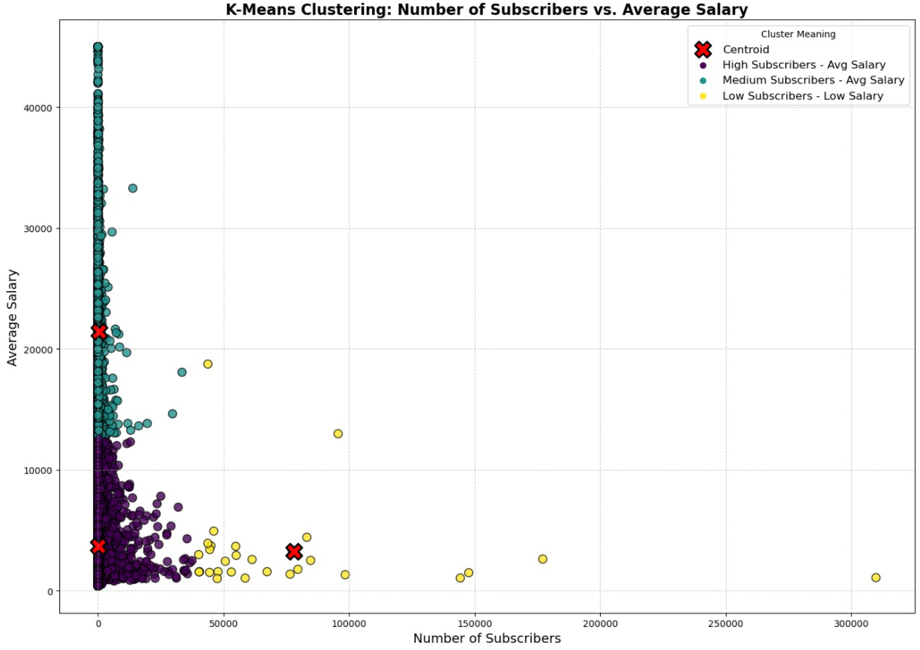
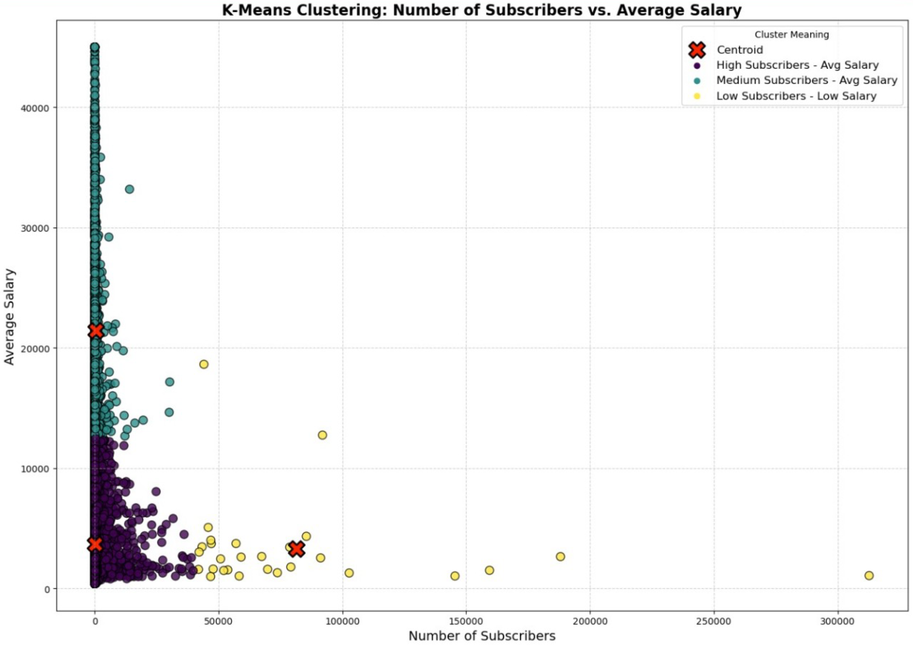
We estimate K-means clusters separately for each quarter (Q1–Q3 2024) using the same setup and $k=3$, allowing for quarter-to-quarter comparison without cross-quarter leakage or pooling effects. Figure 15, Figure 16 and Figure 17 visualize the resulting segments in the subscribers–wage space and mark the learned centroids.

Across quarters, the clusters show a consistent qualitative structure: (i) a segment concentrated at low subscriber counts but spanning a wide wage range (including higher-wage outliers), (ii) a segment with low-to-moderate wages and moderate subscriber counts, and (iii) a smaller segment capturing very large subscriber groups, typically associated with lower wage levels. Most separations are driven by scale (subscriber count) combined with wage dispersion, reflecting compositional differences across aggregated contributor groups.

Caution for Q1

Because Section 3.3 flags a potential Q1 wage anomaly, the Q1 clusters are interpreted as descriptive segmentation rather than definitive wage structure inference, with Q2 and Q3 providing the more stable reference pattern.

7. LLM-Assisted Analysis Layer

This LLM-assisted component is included only as optional reporting support to translate already-computed tables and figures into consistent narrative summaries. The LLM is not used for prediction or forecasting, does not generate new statistics, and does not contribute to any performance claims. This section documents an LLM-assisted analysis layer used to support interpretation and reporting of the empirical artifacts produced in Section 3, Section 4 and Section 5.5. The layer operates only on finalized outputs (tables, figures, and evaluation summaries) to produce concise narrative descriptions for non-technical stakeholders.

7.1. Motivation and Role

Administrative labor market datasets can be large and multi-dimensional, and the empirical workflow in this paper produces multiple artifacts (descriptive plots, correlation matrices, and classification results across Q1–Q3). While these artifacts are reproducible and quantitative, their interpretation can be time-consuming for non-technical stakeholders.

The LLM-assisted layer is introduced for three practical reasons:

• Interpretation support: Generating structured narratives that explain what the already-computed plots and metrics indicate (e.g., where misclassifications occur or how correlations evolve).
• Consistency across quarters: Produceingquarter-by-quarter summaries using the same terminology (salary bands, units in SAR) and the same caveats (the Q1 wage anomaly).
• Interactive querying (optional): Enable a user to ask constrained questions such as “Which age group shows the widest wage dispersion in Q2?” with answers grounded in the existing descriptive figures.

Crucially, this layer is designed to be explanatory, not predictive. Forecasting and prediction in this manuscript relies on explicit statistical/ML models (DT/RF) and their held-out evaluation. The LLM does not replace those models and is not used to produce numerical estimates, parameter values, or new empirical claims.

7.2. Workflow: Chunking, Querying, Aggregation

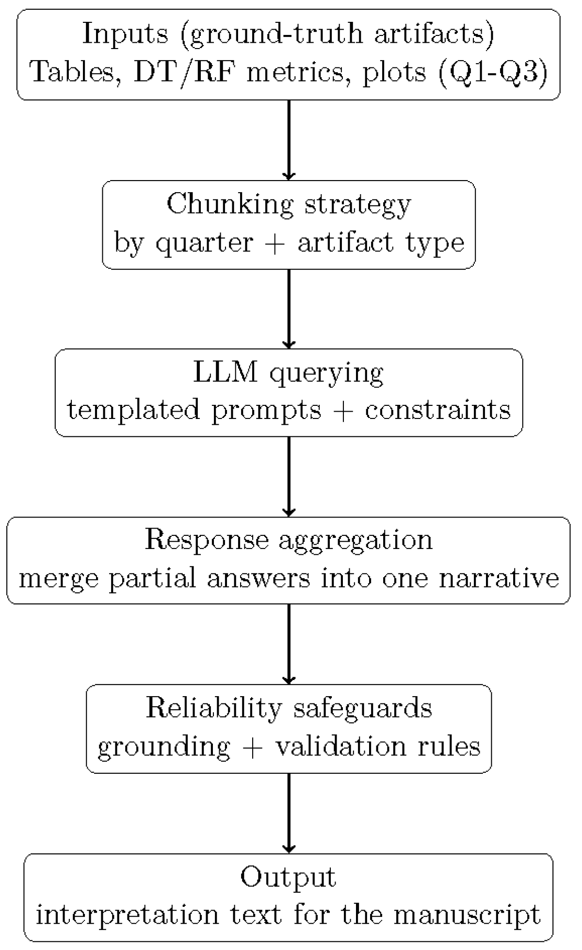
Figure 18 summarizes the workflow. The LLM operates over ground truth artifacts produced by the analysis pipeline (e.g., the wage trend plots, correlation matrices, decision tree visualizations, random forest confusion matrices, and performance tables). The workflow is organized to minimize context mixing and to keep the LLM within manageable input sizes:

• Inputs (ground-truth artifacts): The layer receives only finalized empirical outputs (figures/tables/metrics) and short metadata (quarter, variable definitions, class thresholds). This avoids “free-form” mining of raw tabular data.
• Chunking strategy: Artifacts are grouped by quarter (Q1, Q2, Q3) and type (descriptive, correlation, DT, RF). If a quarter has multiple artifacts, each artifact is summarized independently before synthesis.
• Querying with templates: Prompts follow fixed templates that enforce: (i) consistent definitions (salary bands and units), (ii) non-causal language (descriptive interpretation only), and (iii) mandatory caveats (e.g., flagging Q1 wage anomaly when discussing wage trends).
• Aggregation: Partial responses are merged into a single narrative per quarter, then a short cross-quarter synthesis is produced. Aggregation is rule-based (concatenate + deduplicate + align with section structure), not creative rewriting.
• Validation: The generated narrative is checked against the source artifacts. Any statement that cannot be traced to a table/figure/metric is revised or removed before inclusion in the manuscript.

Figure 18. LLM-assisted analysis workflow. The LLM is used only to translate already-computed empirical artifacts into structured interpretations, not to generate new results or forecasts.

Figure 18. LLM-assisted analysis workflow. The LLM is used only to translate already-computed empirical artifacts into structured interpretations, not to generate new results or forecasts.

7.3. Reliability Safeguards and Limitations

Because LLMs can produce fluent text that may include unsupported details, the LLM-assisted analysis layer is intentionally constrained.

Table 4. Reliability safeguards for the LLM-assisted analysis layer.

Safeguard	Purpose/Rule
Grounding-only inputs	The LLM receives only already-generated artifacts (tables/figures/metrics), not raw full datasets for “free-form” discovery.
No-new-numbers rule	The LLM is not allowed to invent or compute new statistics. Any numeric claim must match an existing artifact or be removed.
Quarter isolation	Prompts and summaries are quarter-scoped (Q1, Q2, Q3) before cross-quarter synthesis to avoid mixing periods.
Template prompting	Fixed prompt templates enforce consistent wording, units (SAR), label definitions, and avoid speculative causal language.
Human validation	All LLM text is reviewed; any statement not directly supported by the empirical section is revised or deleted.
Sensitivity flagging	Known data issues (e.g., Q1 wage anomaly) must be explicitly mentioned in any wage-trend interpretation.
Reproducibility trace	Each narrative paragraph can be traced to specific figures/tables (via figure/table references in the manuscript).

summarizes the safeguards used to keep the LLM outputs aligned with the empirical results.

Limitations. Even with safeguards, the LLM-assisted layer has limitations:

• Not an estimator: This layer does not provide forecasting, causal inference, confidence intervals, or statistical significance.
• Potential sensitivity to phrasing: Small changes in prompt wording can change emphasis; template prompts reduce (but do not eliminate) this effect.
• Dependence on artifact quality: If a figure/table is unclear or incomplete, the LLM cannot fix the underlying empirical gap, only report what is visible in the artifacts.

Implementation note (reproducibility). The LLM-assisted layer can be implemented using any modern LLM API. For reproducibility, the manuscript should report (i) the model family used, (ii) the fixed prompt templates, (iii) chunking rules (quarter/artifact-based), and (iv) the validation rule that prohibits introducing unsupported numbers or claims.

8. Operational Forecasting Oriented Validation

This section evaluates whether the wage-band monitoring signal remains valid when the model is trained on one quarter and deployed on a different quarter. The emphasis is oriented towards operational and forecasting contexts. A model that only performs well under a within-quarter random split may not be reliable for quarterly surveillance, while a model that transfers across quarters provides stronger evidence of stable predictive structure in the administrative release. In addition to point classification metrics, we report probabilistic skill and calibration, since monitoring dashboards typically rely on risk scores and thresholds rather than hard class labels alone.

8.1. Out-of-Time Quarter-to-Quarter Validation

We implement an out-of-time protocol by training the leakage controlled model on one quarter and testing it on a later quarter. This setting mimics real deployment: the model is fit using the last available quarterly release, then used to classify wage bands in the new release when it becomes available. To avoid optimistic evaluation, no pooling is performed across quarters during training and the feature engineering remains strictly leakage-safe.

8.2. Out-of-Time Quarter-to-Quarter Validation

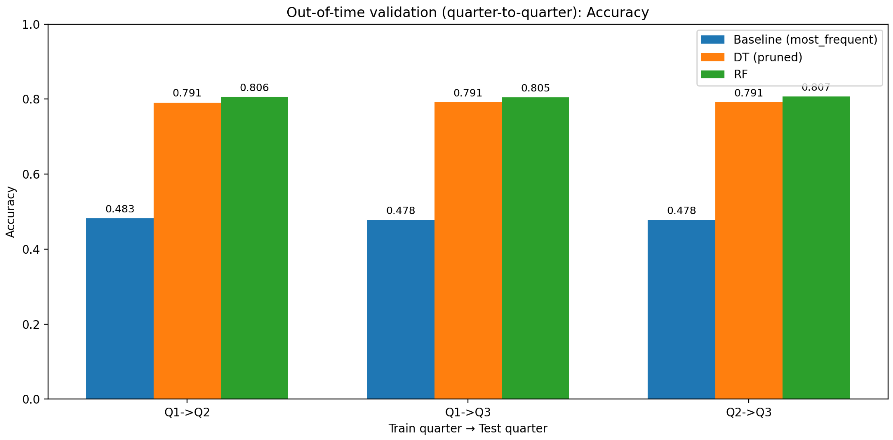
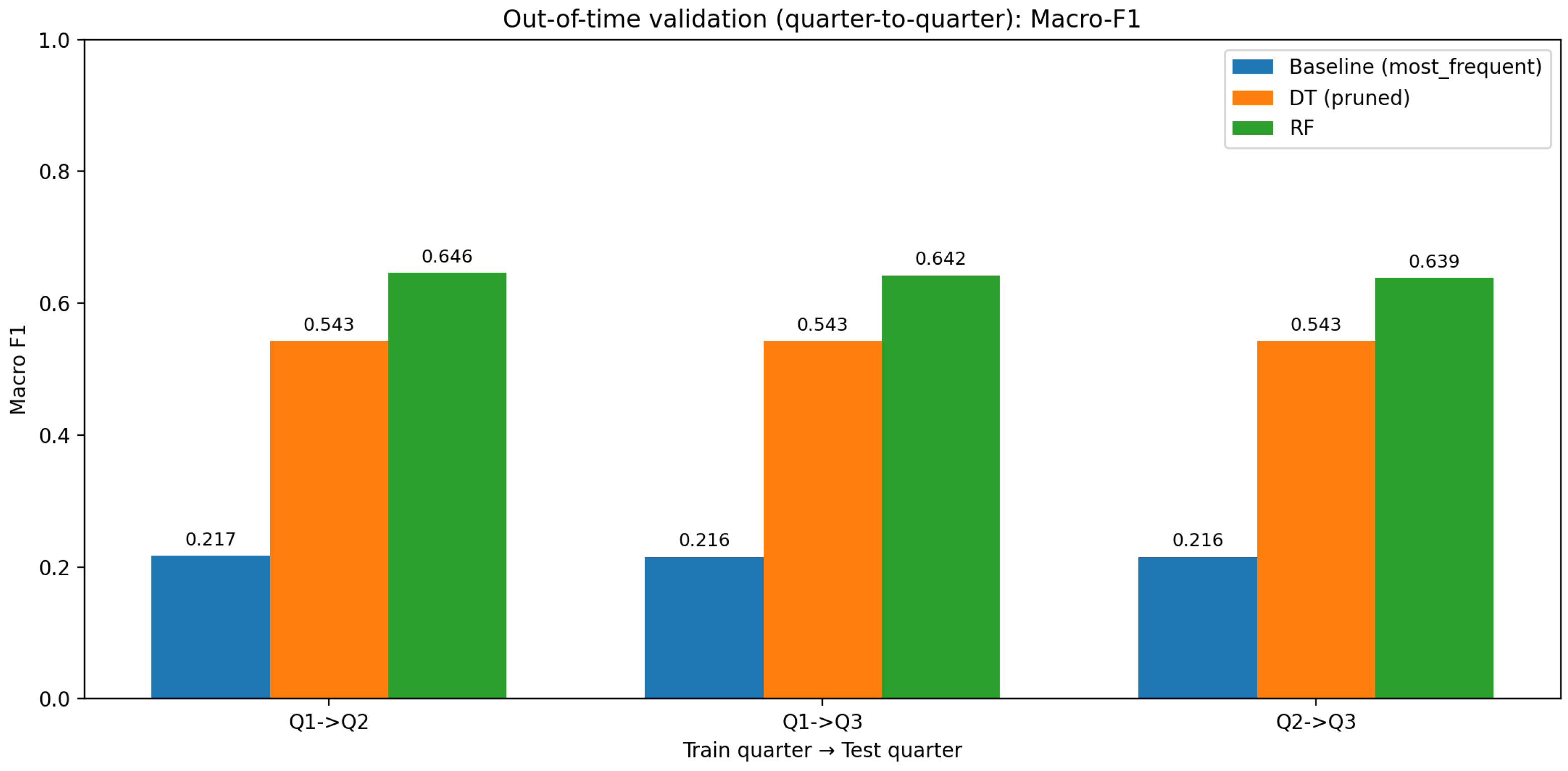
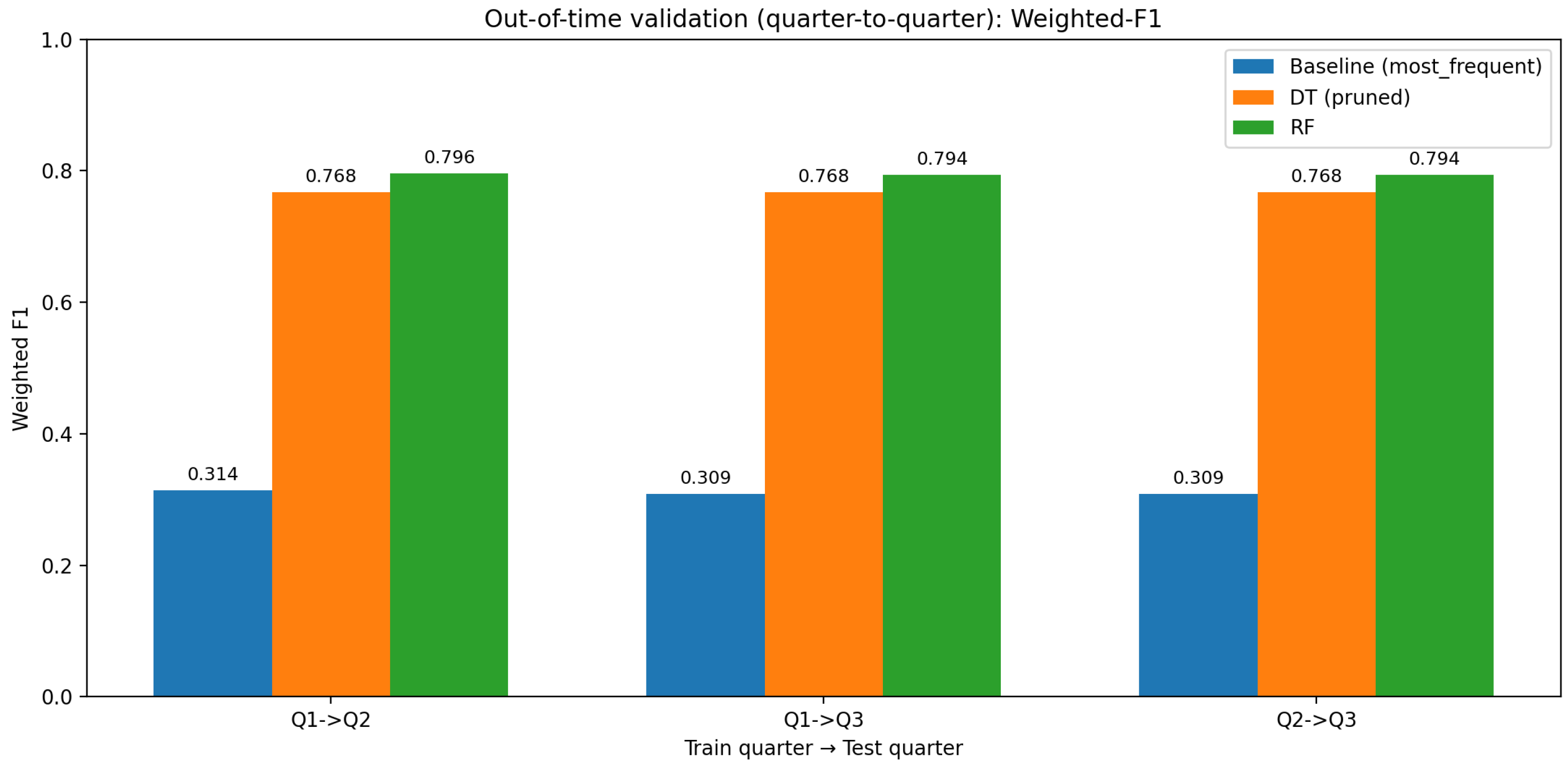
We implement an out-of-time protocol by training the leakage controlled model on one quarter and testing it on a later quarter. This setting mimics real deployment: the model is fit using the last available quarterly release, then used to classify wage bands in the new release when it becomes available. To avoid optimistic evaluation, no pooling is performed across quarters during training and the feature engineering remains strictly leakage safe. For convenience, the exact train→test values are annotated on Figure 19, Figure 20 and Figure 21.

Figure 19, Figure 20 and Figure 21 report out-of-time results for the feasible transfer settings across Q1, Q2, and Q3. Accuracy provides a global view, macro F1 emphasizes balanced performance across wage bands, and weighted F1 reflects performance under class imbalance. Across transfer scenarios, the metrics remain broadly stable, indicating that the learned mapping between administrative descriptors and wage bands persists across releases rather than being an artifact of a single quarter. This stability is important for early warning monitoring, as the objective is to maintain consistent ranking and segmentation quality as new quarterly files arrive.

8.3. Benchmark Baselines and Comparative Reporting

Operational credibility improves when performance is contextualized against simple implementable baselines. Therefore, we include a most frequent class baseline as a strict lower bound that corresponds to a trivial monitoring rule ignoring all covariates. We also include an interpretable pruned Decision Tree as a transparent benchmark that can be translated into explicit rules for segmentation. The out-of-time plots provide the headline comparison visually, while the accompanying comparative table aggregates the full set of metrics for each scenario and supports reproducibility as new quarters are added.

8.4. Robustness via Error Structure Under Distribution Shift

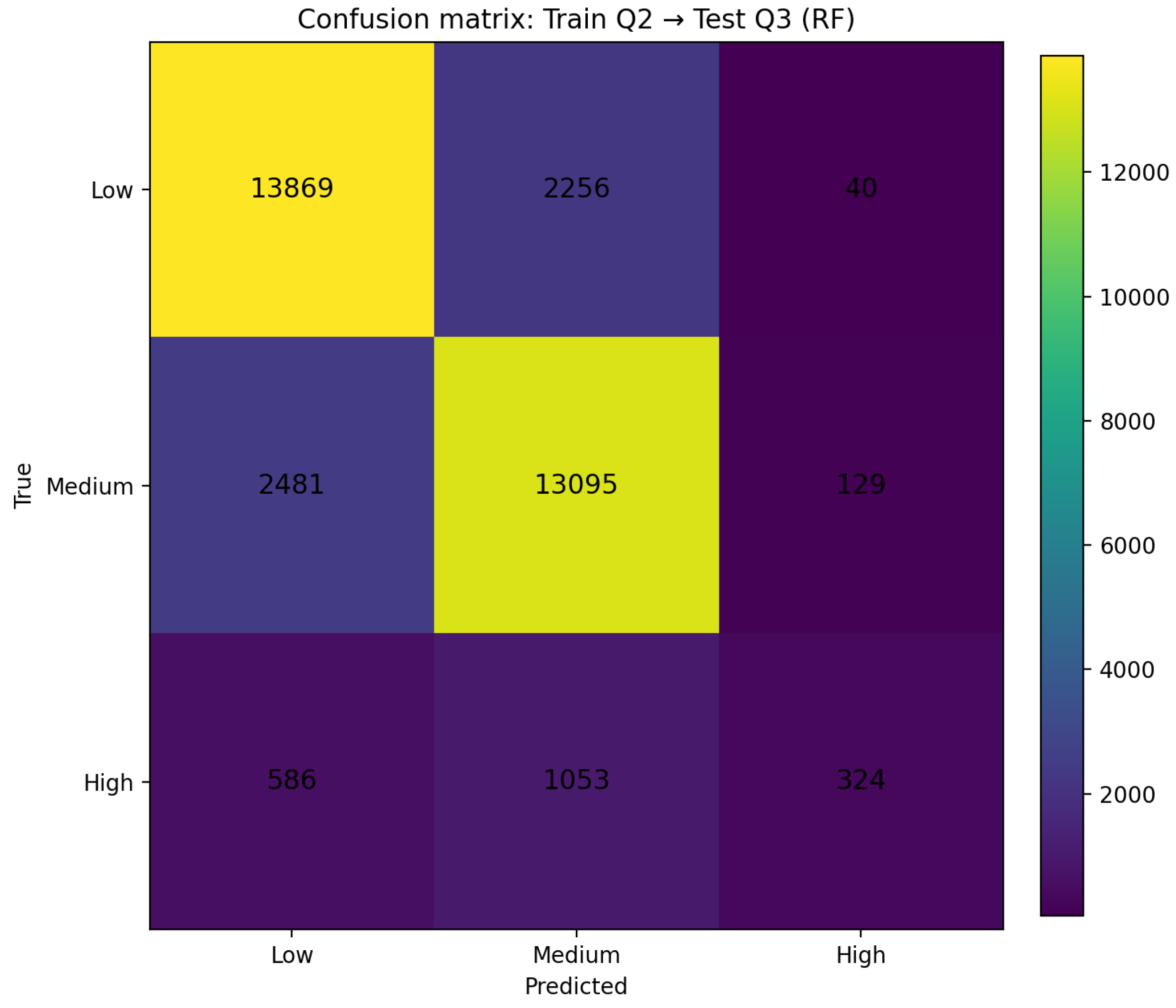
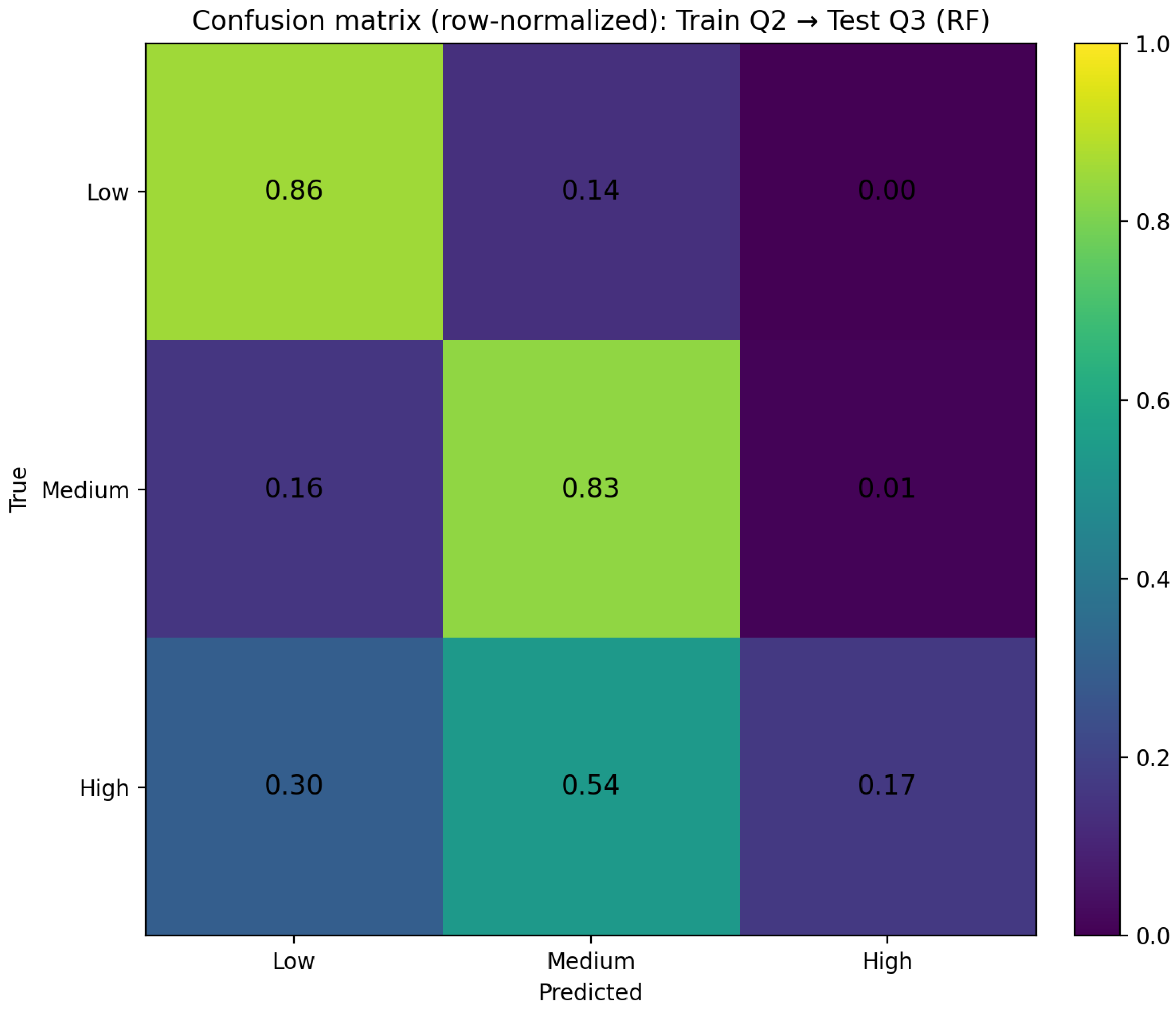
Point metrics summarize overall performance but do not reveal how errors are distributed across wage bands. This matters in monitoring settings, since the cost of misclassification is not symmetric and boundary cases are expected when a continuous wage distribution is discretized into bands. Figure 22 and Figure 23 show an illustrative out-of-time example in which the model is trained on Q2 and tested on Q3 using Random Forest. The counts matrix shows the absolute number of instances in each error category, while the row-normalized matrix clarifies which true classes are most frequently confused.

The dominant confusions occur between adjacent bands, primarily low versus medium and medium versus high, which is consistent with thresholding a continuous outcome. Extreme confusions between low and high are comparatively rare, which is desirable operationally because the monitoring layer is intended to detect broad segmentation rather than fine wage differences near the cutoffs. This error structure supports use of the model as a ranking and triage tool, where groups with higher predicted probability of belonging to the low wage band are prioritized for review.

8.5. Calibration and Probabilistic Skill

Monitoring dashboards often use predicted probabilities rather than only hard labels, for example, to rank groups by risk or to trigger alerts when the probability of being in a low wage band exceeds a chosen threshold. For this reason, calibration is a core forecasting-oriented property. A calibrated model produces probabilities that can be interpreted directly as observed frequencies, enabling threshold-based decision rules that are consistent across time. Calibration is fit using the training split only and evaluated on held-out data to avoid overoptimistic probability estimates; this preserves leakage safety and maintains a deployment-like interpretation of calibrated risk scores.

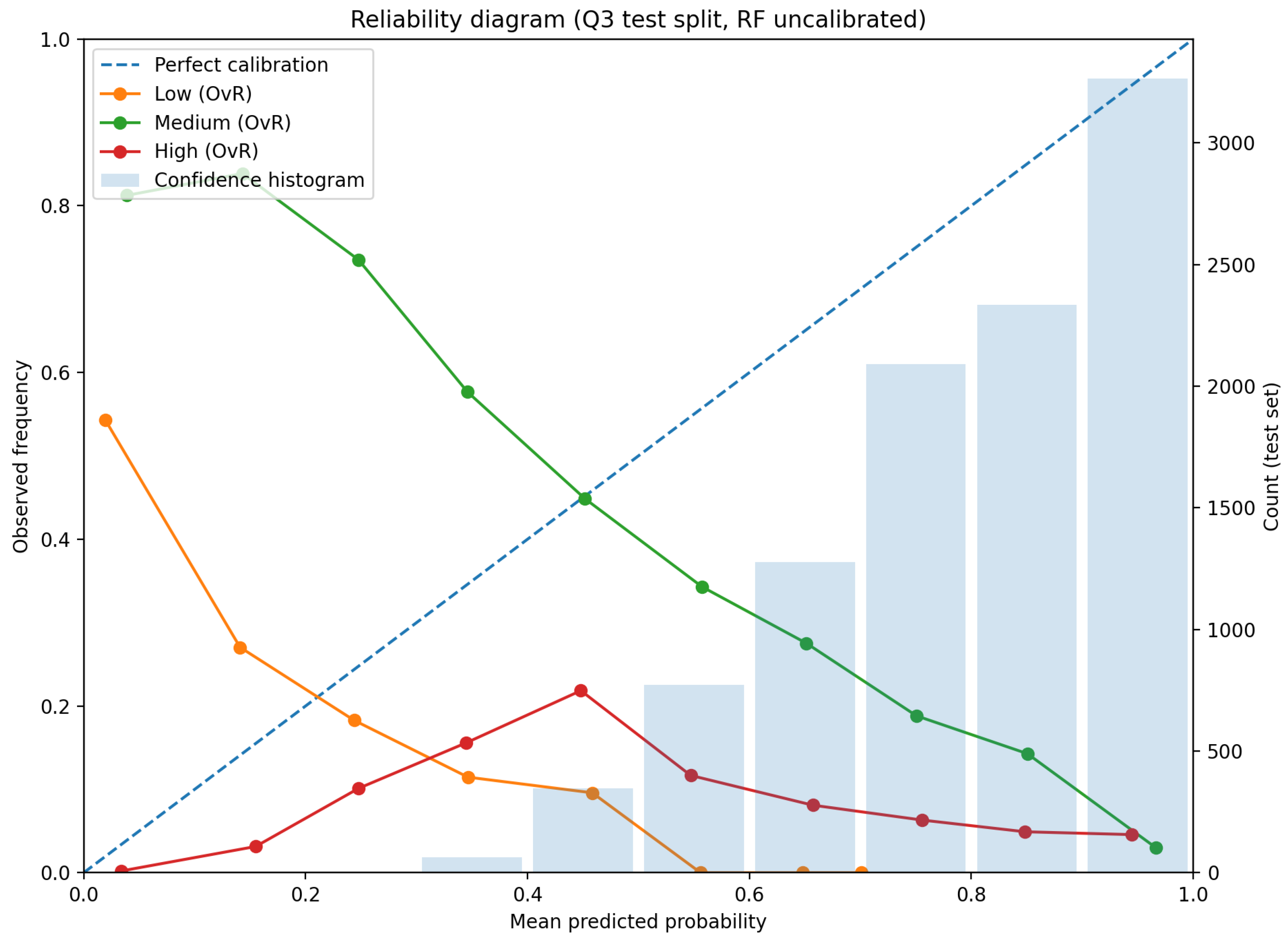
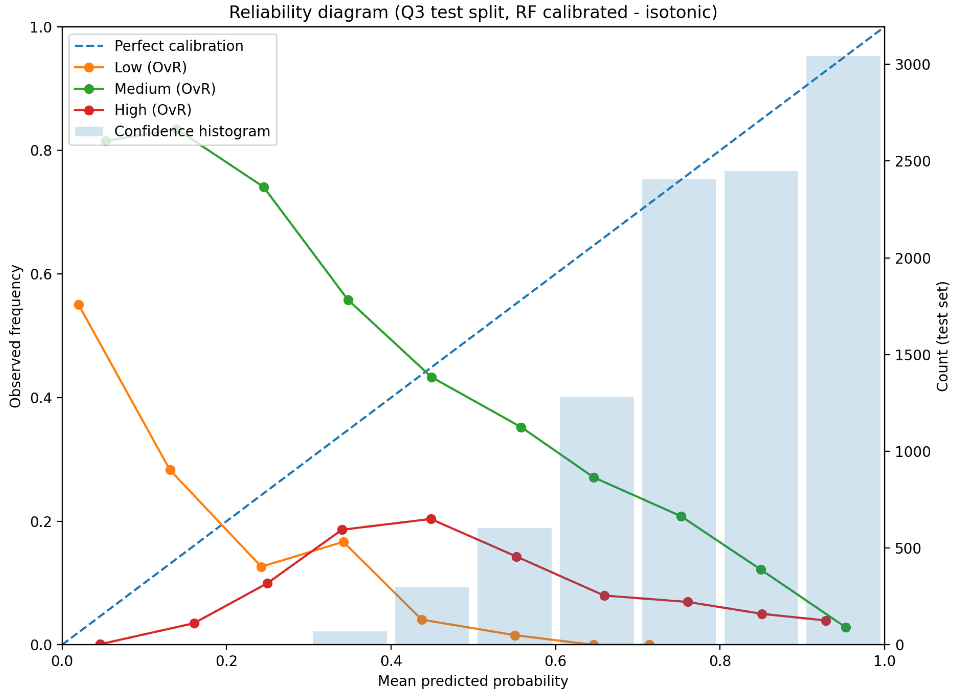
Figure 24 reports the reliability diagram for the uncalibrated Random Forest on the Q3 split using a one-versus-rest view for each wage band. Figure 25 repeats the same assessment after isotonic calibration. The calibrated reliability curves move closer to the diagonal, indicating improved probability interpretability. This improvement matters operationally even when accuracy changes only modestly, because alert thresholds and risk ranking become more stable when probability forecasts are reliable.

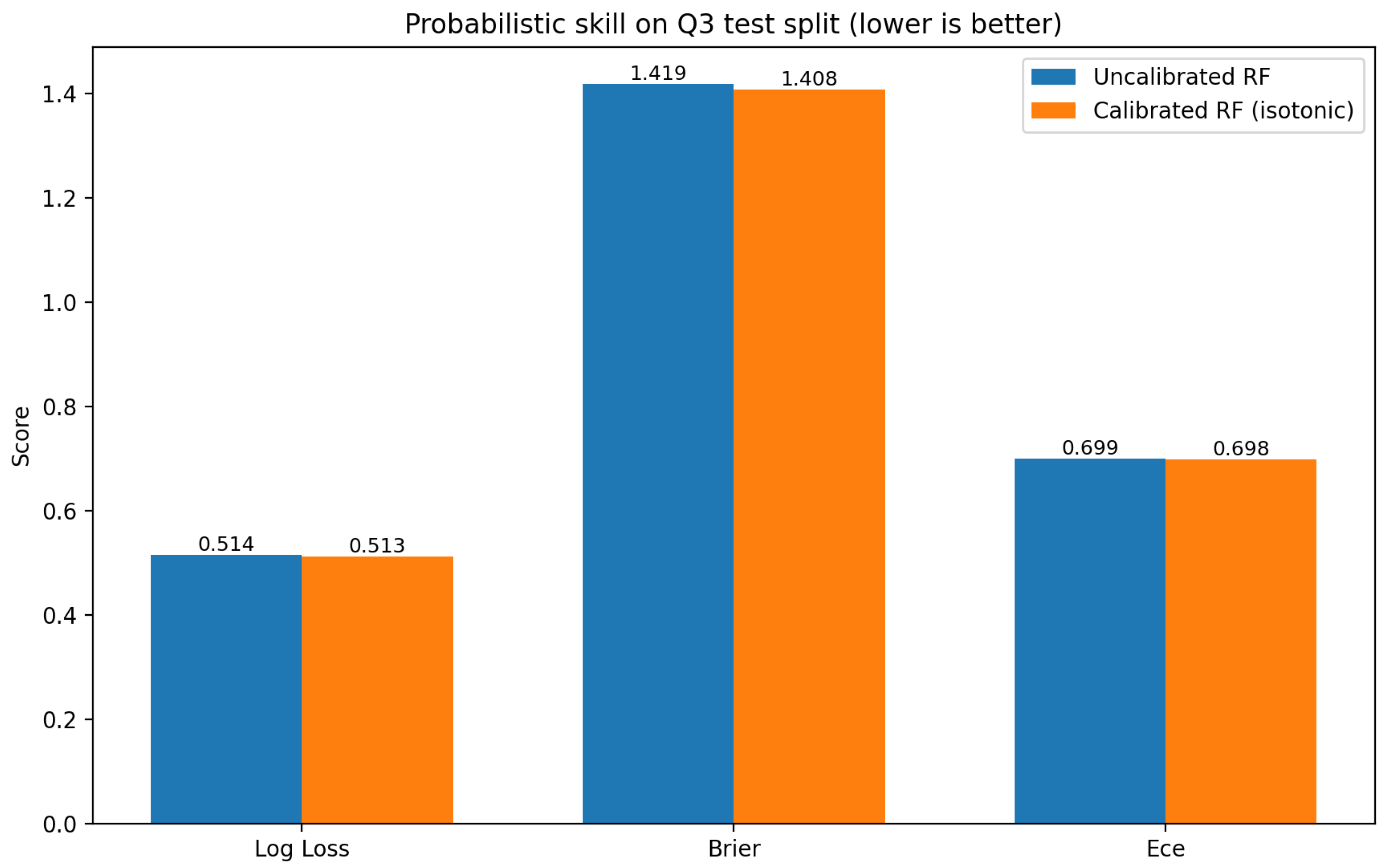
To summarize probabilistic skill numerically, Figure 26 compares proper scoring rules and calibration error for the uncalibrated and calibrated Random Forest on the Q3 split. The log-loss penalizes over confident incorrect predictions, the Brier score measures mean squared probability error, and the expected calibration error provides a compact summary of the calibration mismatch. These measures are standard in probabilistic forecasting and provide a decision relevant complement to accuracy and F1, especially when the model is used as a risk scoring layer in an early warning dashboard.

8.6. Error Cost Framing for Monitoring Decisions

The operational cost of misclassification depends on how the monitoring output is used. If the goal is early warning, then missing a truly low wage segment can be more costly than incorrectly flagging a medium wage segment, because false negatives delay attention. If the model is used to allocate limited resources, excessive false positives can dilute capacity. These asymmetric costs motivate probability thresholding rather than relying solely on the maximum probability class. The calibrated probability outputs together with the confusion structure observed under out of time transfer support a monitoring design in which analysts choose thresholds that reflect policy priorities and capacity constraints, then track how those thresholds perform as new quarters are released. Operationally, a monitoring dashboard can select a probability threshold (e.g., $P\left(\mathrm{Low}\right)>\tau$) to control the tradeoff between detection and false alarms; lower $\tau$ increases sensitivity but raises alert volume, while higher $\tau$ reduces false alarms at the cost of missed detections.

Overall, the results in this section demonstrate that the monitoring signal is not confined to within quarter evaluation, that it transfers across quarterly releases, and that probability-based outputs can be assessed and improved using calibration methods and proper scoring rules. This aligns the framework more closely with forecasting practice while remaining consistent with leakage control and administrative data constraints.

9. Discussion and Implications

This section interprets the main empirical findings from the descriptive evidence (Section 4), the predictive modeling exercises (Section 5), and the operational forecasting-oriented validation results (Section 8). The discussion emphasizes what can be learned from quarterly administrative monitoring, how the observed age and sector patterns should be interpreted in a policy-relevant way, and how the additional validation layer clarifies what does and does not generalize when models are transferred across quarterly releases under realistic information constraints.

9.1. What Quarterly Monitoring Reveals That Annual Reports Miss

Quarterly administrative data can surface short-horizon dynamics that are difficult to detect in annual reporting cycles, both in substantive labor-market signals and in data quality behavior. The Q1–Q3 sequence makes it possible to observe whether changes are gradual, accelerating, or reversing within the year. In our data, contributor totals increase from Q1 to Q3, which is operationally relevant for near-term planning because it reflects current participation rather than retrospective conditions. Quarterly monitoring also improves the visibility of reporting artifacts: the Q1 wage anomaly illustrates that higher-frequency review can flag inconsistencies early, before they become embedded in annual aggregates and distort interpretation.

The forecasting-oriented value of quarterly releases is not limited to descriptive tracking. Quarterly measurement supports predictive monitoring that can be executed repeatedly as each release arrives, and it enables validation under operational constraints. The out-of-time validation in Section 8 complements within-quarter train–test evaluation by explicitly testing whether a model trained on one quarter transfers to the next quarter without using future information. This distinction matters for practice; a model that performs well only under within-quarter random splits may still fail when confronted with the distributional shifts, reporting idiosyncrasies, or compositional changes that occur between releases.

9.2. Interpretation of Sector and Age Patterns

The descriptive evidence highlights heterogeneity across age groups and sectors that is concealed by aggregate averages. Mid-career cohorts (26–40 and 41–59) exhibit the largest dispersion, which is consistent with a broader mix of occupations, seniority, and sectoral placements. For monitoring, dispersion is informative in its own right; a stable mean wage can coexist with widening heterogeneity across subgroups, meaning that quarterly dashboards should track distributional behavior and not only point estimates.

Sectoral growth is most defensibly interpreted as compositional at the aggregation level available in the GOSI releases. Changes can reflect expansion in registered establishments, shifts in job composition within categories, or administrative changes in reporting and registration behavior; thus, quarterly patterns should not be over-interpreted as within-sector productivity change or within-job wage growth without additional covariates. The predictive models reinforce this view. Under leakage control, salary class is only moderately predictable from administrative descriptors (age group, entity type, nationality, and subscriber counts), which indicates that wage class is not a deterministic function of the observed categories and that unobserved heterogeneity remains important.

The operational validation layer clarifies how these relationships behave when moving from one quarter to the next. Out-of-time transfer performance provides a more realistic test of whether the learned signal is stable enough for repeated quarterly deployment. In addition, probabilistic assessment and calibration address a practical monitoring need that accuracy alone cannot satisfy: if the output is used to trigger investigation or prioritization, then decision makers need reliable probabilities, not just hard labels. Therefore, the reliability plots and calibration skill comparison in Section 8 strengthen the monitoring interpretation by showing whether predicted risks are meaningfully aligned with observed frequencies under a realistic deployment split.

9.3. Limitations and Generalizability

Several limitations constrain inference and should be made explicit to avoid over-interpretation. The Open Data Portal releases used here are aggregated by combinations of administrative and demographic categories; thus, the analysis is group-level and cannot support individual-level statements. This also limits causal interpretation because changes in average wage within a group can reflect compositional changes rather than wage changes for the same individuals. These constraints motivate a careful framing: the contribution is operational monitoring and predictive segmentation, not causal evaluation of reforms.

The time horizon is short (three quarters), which is appropriate for demonstrating the value of quarterly monitoring but insufficient for seasonal adjustment, structural change detection over multiple business cycles, or robust forecasting of future quarters. The operational validation results partially mitigate this limitation by testing quarter-to-quarter transfer, but do not replace multi-year evaluation. Extending the framework to multiple years is necessary in order to separate seasonal hiring patterns from persistent trends and establish whether the quarter-to-quarter transfer remains stable across different macroeconomic phases.

Data quality constraints remain central. The Q1 wage anomaly requires cautious interpretation when discussing wage trends across Q1–Q3, and the missing wage entries in Q2 and Q3, while few, could still be non-random in ways that affect subgroup summaries. A related operational limitation is that administrative releases can change definitions, reporting rules, or category codings over time. Even when the schema appears stable, small changes can induce distribution shifts that matter for model transfer and calibration. This is one reason the out-of-time evaluation and the robustness emphasis in Section 8 are important, and can also motivate future work on monitoring distribution shift, anomaly detection, and revision-aware pipelines.

Feature limitations also constrain performance. The leakage-controlled models deliberately exclude salary-derived predictors, which keeps evaluation credible but makes the task inherently difficult. Therefore, moderate predictive accuracy should be interpreted as a realistic signal level available from the published descriptors, not as an upper bound on what is possible. Improving skill, particularly for the High class, likely requires richer covariates that remain policy-relevant and operationally available, such as occupation composition proxies, education structure, firm size distribution, regional price indices, or local economic activity indicators. In a monitoring context, probabilistic calibration is equally important; even when discrimination is moderate, calibrated probabilities can still support decision rules that are transparent and cost-aware. In particular, improving separation for the High wage band likely requires additional leakage-safe covariates that remain operationally available, such as economic-region context, sector-level indicators, or macro conditions (e.g., inflation), potentially integrated from auxiliary public sources.

External validity should be treated cautiously. While the methodological point that higher-frequency administrative monitoring improves timeliness is general, empirical patterns depend on the structure of the Saudi labor market as well as on how GOSI aggregates and publishes categories. Generalization to other countries requires adapting to local administrative definitions, while generalization to other years within Saudi Arabia requires multi-year validation to account for changes in institutional reporting practices and labor market conditions. Within these constraints, the present study provides a reproducible template for quarterly surveillance that combines descriptive monitoring, leakage-controlled predictive segmentation, and operational validation intended to better match how a quarterly pipeline would be used in practice.

10. Conclusions and Future Work

This paper uses quarterly GOSI administrative releases (Q1–Q3 2024) to demonstrate how higher-frequency labor market measurement can support timely forecasting-oriented monitoring under Saudi Vision 2030. Contributor counts rise steadily from roughly 11.39 M in Q1 to 12.01 M in Q3 (+5.6%), while wages show modest movement from Q2 to Q3 (SAR 4615 to SAR 4647) alongside an early-year Q1 wage level anomaly that warrants cautious interpretation and motivates explicit data quality handling in any monitoring pipeline. Disaggregated evidence indicates meaningful heterogeneity by age group, with the largest wage dispersion concentrated in mid-career cohorts, along with correlation patterns that remain stable across quarters, supporting the feasibility of quarter-by-quarter surveillance that is operationally consistent. On the predictive side, we formulate a leakage-controlled salary class classification task to assess whether non-salary administrative descriptors can anticipate low/medium/high wage bands. An interpretable Decision Tree yields stable but moderate performance and a Random Forest improves robustness, with most residual errors occurring between adjacent wage bands, consistent with discretization of a continuous wage distribution and indicating that richer covariates such as occupation mix, education, firm characteristics, and local economic conditions are needed for stronger predictive separation. To align evaluation with operational use, we also introduce out-of-time quarter-to-quarter validation and probabilistic assessment, showing that skill transfers across releases and that calibration improves the reliability of predicted probabilities for threshold-based monitoring and early warning dashboards. As additional quarterly releases accumulate, the pipeline can be extended from predictive monitoring toward forecasting by implementing a rolling nowcasting setup (train on recent quarters and predict the next release upon arrival; for example, train on Q1–Q2 and evaluate on Q3 as the next-release test bed), introducing lagged administrative indicators and quarter-ahead forecasts with uncertainty quantification, and adopting hierarchical forecasting across region–sector–age aggregation levels while monitoring for structural breaks and reporting artifacts. Looking forward, two extensions are especially promising: first, beyond band classification, forecasting wage distributions (e.g., quantiles) rather than only averages would better capture dispersion dynamics across subgroups; second, the Q1 anomaly motivates integrating automated anomaly detection and revision-aware modeling so that the pipeline remains robust to administrative reporting artifacts. Finally, the LLM-assisted layer should remain an interpretation interface rather than a forecasting engine, constrained to explain validated computed outputs (tables and figures) within an auditable and reproducible quarterly workflow.