A Combined Kalman Filter–LSTM to Forecast Downside Risk of BWP/USD Returns: A Bottom-Up Hierarchical Approach

Highlights

What are the main findings?

• A Combined Kalman Filter–LSTM architecture significantly improves the forecasting of downside risk in BWP/USD returns by capturing both time-varying state dynamics and nonlinear temporal dependencies.
• The proposed bottom-up hierarchical approach enhances forecast consistency across aggregation levels and yields superior predictive accuracy relative to standalone Kalman Filter and LSTM specifications.

What are the implications of the main findings?

• Integrating state-space filtering with deep learning provides a robust methodology for modelling asymmetric and tail risk in emerging foreign exchange markets.
• The framework offers practical value for exchange rate risk management, monetary policy surveillance, and financial stability monitoring in small open economies such as Botswana.

Abstract

This paper offers a hybrid forecasting approach that merges a local-level state space Kalman filter with a Long-Short-Term Memory (LSTM) neural network to assess the downside risk of the Botswana Pula versus the US Dollar (BWP/USD). Inspired by the inability of conventional econometric models to capture complex latent structural shifts and nonlinear patterns, our architecure uses a bottom-up hierarchical methodology in which the smoothed level component of the exchange rate is isolated by the Kalman filter and subsequently fed into the LSTM architecture. Three key indicators for assessing downside risk—Maximum Drawdown (MDD), Conditional Drawdown-at-Risk (CDaR), and Downside Deviation—are used to assess model performance across various time-frames (7, 30, 90, 180, and 240 days). As confirmed by Kupiec and Christoffersen’s backtesting processes, the findings show a high degree of alignment between projected and actual values, with negligible downside deviation bias and robust calibration. Moreover, global economic and geopolitical shocks, such as the COVID-19 pandemic, the Russia–Ukraine conflict, and the 2015–2016 Shanghai Stock Exchange crash, are important factors that influence exchange rate volatility, according to explainable artificial intelligence techniques, particularly SHAP (SHapley Additive exPlanations) analysis. Downside risk is also greatly increased by regional currency links, especially the impact of the ZAR/BWP exchange rate. On the other hand, domestic temporal variables, such as week, quarter, and month, have very little impact. These results emphasise how Botswana’s currency rate is structurally vulnerable to external shocks and how crucial it is to include both global and regional considerations in risk analysis. The research concludes that the accuracy and transparency of projections for exchange rate risk significantly improve when practical filtering is combined with deep learning and explainable AI. To improve macroeconomic resilience and guide successful financial risk management plans in emerging market environments, policymakers are advised to employ AI-driven forecasting techniques, enhance regional monetary coordination, and set up real-set learning systems.

1. Introduction

A risk measure may be thought of as a map from the space of probability distributions to actual numbers from the perspective of financial risk managers. By employing risk measurements to assign precise amounts for possible losses to banks and other financial institutions, risk management specialists can modify their capital buffers against downside risk. The foreign exchange market is the largest and most liquid financial market in the world, with an average daily turnover of 5.1 trillion US dollars. Given that exchange rates fluctuate widely, accurate forecasting of exchange-rate volatility is important to financial institutions and traders aiming to hedge currency [1]. Similarly, with foreign exchange options, traders aim to earn by purchasing or disposing of options if they anticipate volatility to surpass (decline) the indicated value of currency-option premiums. Furthermore, a substantial amount of theoretical research has connected trade with exchange-rate volatility. Researchers such as [2] have long used several stylised facts, including time-varying, volatility clustering, and persistence, to characterise the volatility of financial asset returns. Ref. [3] offered the ARCH (herein referenced autoregressive conditional heteroscedastic) model, whereas ref. [4] promoted the GARCH (generalised ARCH) model as a solution to these stylised phenomena. Since then, a range of GARCH models have dominated the volatility forecasting framework, particularly the asymmetric GARCH models. According to [5], the GJR-GARCH model is a straightforward family of GARCH models that can capture the leverage effects of both positive and negative news on conditional volatility. Investors, legislators, and other stakeholders must comprehend and forecast the downside risk of the foreign exchange rate market to evaluate possible losses and make well-informed choices. The growing complexity and interconnectivity of global markets demand increasingly sophisticated modelling methodologies, even though many studies have used a variety of statistical and econometric tools to model and forecast downside risks; see, for instance, [6,7]. Understanding how inflation affects foreign exchange market risks makes this environment much more complex. In times of high inflation, the connection between inflation and foreign exchange market risks becomes even more important, making it a crucial factor to take into account when making investment and policy decisions. Considering the different stages of the world economy, 2010 was characterised by comparatively low inflation in different parts of the world. However, after 2020, there was a spike in high inflation, exacerbated by the COVID-19 epidemic. This inflationary landscape has been shaped by elements that include labour market changes, energy price swings, and supply chain interruptions [8].

In response to this complex backdrop, this study presents a new application for forecasting possible losses (downside risks), in the foreign exchange market during these times of high inflation. To investigate statistical dependencies under various inflationary settings, data are segmented by acknowledging the theoretical difficulties of developing prediction models by randomly mixing data in the case of time series. This offers a thorough analysis of various hierarchical environments. Specifically, a bottom-up hierarchical approach that takes into account the notable changes in foreign exchange markets is performed in this study to acknowledge the need to forecast using a high-frequency time series that is less skewed. This method takes into account the effects of hierarchies and uses a network-based perspective to capture the intricate dynamics of the BWP/USD. Furthermore, the use of conditional statistical dependencies, a technique that investigates the reciprocal impact of hierarchies in light of the present financial changes, provides important insights into the complexity and dynamic character of this currency. This methodology uses hierarchies as the conditioning variables, and therefore applies the combined Kalman filter–LSTM to nonlinear mutual dependencies; whereas, ref. [9] took a different approach and introduced the entropic value-at-risk (EVaR) as a coherent measure of downside risk, and benchmarked with the maximum drawdown, the Sortino ratio, and the marginal expected shortfall which are used to measure downside risk.

With these facts, the main contribution of this study is the development of a new and robust methodological application for foreign exchange risk forecasting. Specifically, we integrate a Kalman filter with long short-term memory networks within an AWS (Amazon Web Services) environment for real-time implementation. This application is designed to enhance the accuracy of downside risk forecasts—particularly in the BWP/USD market. For real-time deployment and assessment, we leverage AWS EC2 instances, which provide scalable and flexible high-performance computing (HPC) capabilities, and AWS Lambda functions, which enable cost-efficient, event-driven execution without the need for server management. By combining HPC resources with serverless computing, the proposed application achieves both the computational power required for intensive model training and the agility needed for rapid, on-demand risk evaluation, making it highly adaptive to dynamic market conditions. Antagonistic to preceding work such as that by [10], which used statistical or machine learning models, this study combines both approaches to better address the nonlinearity, noise, and volatility clustering that occur in high-frequency exchange rate data. To address the irregular and multi-scale dynamics of BWP/USD, temporal hierarchies (i.e., weekly, monthly, quarterly, half-yearly, yearly) alongside key exogenous variables such as macroeconomic indicators (inflation, interest rates), geopolitical shocks (COVID-19 pandemic, Russia–Ukraine war), and related financial variables (e.g., ZAR/USD) are also included. This bottom-up hierarchical conditioning results in forecasts that are not only coherent across multiple aggregation levels but also sensitive to structural shifts and crises.

Finally, the inclusion of the prediction intervals plays a critical role in enhancing the practical relevance, reliability, and interpretability of the forecasts of the architecture. Unlike point forecasts, which provide only a single estimated value, prediction intervals offer a range, within which the true future values are expected to fall with a specified level of confidence. This distinction, according to [11], is crucial when modelling volatile financial series, where uncertainty is inherent and extreme movements can have significant economic consequences. Hence, assessing the model stability through prediction intervals in this study ensures that the Kalman filter–LSTM architecture is not merely fitting historical data but is genuinely capable of generalising to unseen data under various market conditions. The ability of this architecture to maintain tight and stable prediction intervals without frequent violations is indicative of its resilience, reliability, and real-world applicability. Additionally, this combination significantly enhances the forecasting of nonlinear mutual dependencies in currency markets, particularly in the context of high-frequency financial data like the BWP/USD currency pair. The Kalman filter is adept at filtering out noise from high-frequency data, which is often volatile and subject to random fluctuations. By preprocessing the data with a Kalman filter, the LSTM model receives cleaner input, allowing it to focus on underlying trends and patterns rather than being misled by noise. This noise elimination, according to [12], leads to improved performance in extracting hidden patterns in financial time series, as evidenced by studies showing substantial gains in prediction accuracy when using Kalman filtering alongside LSTM. Moreover, with the Kalman filter, the aim is to provide a recursive method for estimating the state of a dynamic system over time. Continuously updating predictions based on new observations allows real-time adjustments that enhance the ability of LSTM to capture temporal dependencies and changes in market conditions. This dynamic state estimation is crucial for accurately modelling the nonlinear relationships inherent in currency movements [13]. The synergy between Kalman filtering and LSTM networks creates a robust model for forecasting in the foreign exchange market. By effectively reducing noise, dynamically estimating states, managing nonlinear dependencies, and improving stability, this combination offers significant improvements over forecasting methods, enabling better risk management and decision-making in currency trading contexts. To further improve the generalisability of our application, we also contrast the performance of the LSTM with that of the Transformer model. This comparative analysis allows us to highlight the advantages and limitations of both architectures, ensuring that our findings remain broadly applicable across different modelling approaches.

2. Research Highlights and Key Findings

While specific studies on a Kalman filter–LSTM approach targeting downside risk in BWP/USD returns using a bottom-up hierarchical methodology are lacking, foundational insights from previous research on Kalman–LSTM hybrid architectures and hierarchical forecasting provide a conceptual basis. This study is therefore novel in developing a combined methodological application that integrates these components, yielding valuable contributions to financial forecasting and risk management. The research highlights and key findings are summarised below.

• Combination of Kalman filter and LSTM via Stacked Architecture:
  The hybrid Kalman filter–LSTM model achieved the lowest forecasting errors among evaluated models, demonstrating enhanced downside risk prediction and strong generalisation to out-of-sample BWP/USD data.
• Hierarchical Forecasting Structure:
  A bottom-up temporal hierarchy captured downside risk dynamics across multiple aggregation levels (weekly to yearly), ensuring forecast coherence and improved risk resolution at different time scales.
• Targeted Focus on Downside Risk:
  Analysis based on Maximum Drawdown, Sortino Ratio, and Marginal Expected Shortfall revealed substantial downside exposure in BWP/USD returns, especially over medium- and long-term forecast horizons.
• Robust Backtesting and Risk Validation:
  Kupiec and Christoffersen tests confirmed the statistical validity of the predicted tail risk measures at critical quantile thresholds (1%, 5%, 95%, and 99%).
• Explainability via SHAP Analysis:
  SHAP-based interpretability assessment identified monetary policy shocks, the Russia–Ukraine conflict, the COVID-19 pandemic, and ZAR/USD exchange rate dynamics as key drivers of BWP/USD volatility.
• Incorporation of Prediction Intervals:
  Forecast uncertainty was quantified using 99.9% prediction intervals, with observed BWP/USD returns largely contained within these bounds, confirming the model’s reliability and stability.
• Scalable Framework for Broader Financial Contexts:
  The proposed hybrid methodology is adaptable to other financial assets, such as currency pairs, commodity prices, and equity indices, making it broadly applicable to high-volatility financial environments.

The rest of this paper is as follows: Section 3 presents methods and procedures used in the study. Section 4 discusses the study’s empirical analysis, while Section 5 presents the discussion, conclusion, and recommendations.

3. Materials and Methods

This section presents the study’s techniques and processes. The suggested system uses incoming exchange analysis to create a combined forecasting architecture for the five-day Botswana Pula versus the US dollar (BWP/USD) in real-time. The system is composed of two parts for the BWP/USD downside risk forecasting scenario. The two parts are explained and discussed in Section 3.1 and Section 3.1.3, respectively.

3.1. Data Source and Designing a System for Data Pre-Processing

This component provides the data to the analytical server for forecasting downside risk and is responsible for its efficient use. The Python high-performance computing is the primary component of the system setup. TensorFlow is utilised because it is compatible with Python (version 3.11), JavaScript (ES2022), C++ (C++20), and Java (version 21), among other programming languages. According to [14], this adaptability makes it suitable for various uses across several industries. A comma delimiter is used to separate the fields in a raw data file. The analytical server receives the raw data file to construct a forecasting architecture. This makes the system exceptionally versatile, assists in building a solid self-learning architecture on a real-time basis, is highly scalable and helps to build a strong self-learning forecasting architecture.

3.1.1. External Variables: Definitions and Data Sources

This study implements a Bottom-Up Hierarchical Time Series (BUHTS) framework to improve predictive accuracy and account for the multiscale characteristics of financial time series. This structure facilitates the integration of internally derived components from the BWP/USD exchange rate series with externally sourced macroeconomic and geopolitical indicators. Each component is analysed as a disaggregated series at the lower hierarchical level and later aggregated to create the final forecasting input. Based on a bottom-up disaggregated time hierarchy, the BWP/USD exchange rate is broken down into a number of interpretable time series components for the internal structure. Daily trends, weekend impacts, and more general seasonalities, including monthly, quarterly, semi-annual, and yearly cycles, are some examples of these elements. These components are extracted using classical decomposition, which captures a variety of temporal characteristics within the series. The forecasting model can identify and use significant signals across a variety of time scales thanks to this hierarchical decomposition, which also maintains the integrity of the time series.

In parallel, external variables known to influence currency movements are introduced into the hierarchical system. These include: (1) COVID-19 Daily Cases (Botswana): Sourced from Our World in Data, this variable captures the health shock intensity over time (Accessed on 28 May 2025). (2) 2015–2016 Shanghai Stock Market Crash: Treated as a shock dummy, this event is captured based on market timing identified in financial archives and summaries provided by public resources like Wikipedia. Using web scraping and text mining techniques, such as topic modelling via Latent Dirichlet Allocation (LDA), we were able to extract this data on https://www.investopedia.com/articles/investing/022716/4-consequences-government-intervention-chinas-markets.asp; (Accessed on 29 May 2025). (3) Russia–Ukraine War Indicator: A binary variable marking the onset and persistence of the conflict, obtained from web scraping the following website https://www.russiamatters.org/news/russia-ukraine-war-report-card/russia-ukraine-war-report-card and processing the text data using text mining techniques such as topic modelling via LDA and during the period from 24 February 2022 to 27 May 2025 (accessed on 29 May 2025). (4) Interest Rate (Botswana): The Bank of Botswana’s official policy rate, sourced from the Bank of Botswana, was resampled to daily frequency to match the daily BWP/USD exchange rate; (accessed on 28 May 2025). (5) Inflation Rate (Botswana): Monthly inflation rates based on Consumer Price Index (CPI) changes were retrieved from Statistics Botswana, then adjusted to daily granularity; (accessed on 28 May 2025). (6) ZAR/BWP Exchange Rate: Daily exchange rates between the South African Rand and Botswana Pula were collected from Yahoo Finance( accessed on 28 May 2025). (7) Investor sentiment was quantified using weekly data from the American Association of Individual Investors (AAII) Sentiment Survey. The survey captures the percentage of individual investors who are bullish, bearish, or neutral on the stock market over the next six months. These data were obtained through automated web scraping of the AAII website https://www.aaii.com/sentimentsurvey, allowing us to track market sentiment over time and align it with exchange rate dynamics; (accessed on 12 June 2025).

3.1.2. Problem Definition

Assuming the original time series is denoted as $X_t$, a state space Kalman filter is applied to reduce the noise in this series, yielding a smoothed trend denoted as s. Given a time series r, its set of sliding windows is extracted to construct the training dataset. Let each window be of length n, and the corresponding training labels be denoted as Y. These windows, according to [15], serve as input features for the learning architecture, allowing it to capture the temporal dynamics of the denoised series for forecasting or classification tasks. The algorithm needs to learn a function f that is defined as

$$f:\{s_1,s_2,\dots ,s_n\}\to Y.$$

(1)

Thus, the solution is formally defined as

$$\widehat{f}={\displaystyle \frac{1}{N}}\sum _{i=1}^{N}f(s_i;\theta )$$

(2)

where $\widehat{f}$ is the parameter set of model f and N is the size of the training set. The LSTM and the Transformer encoders are used in this study to interpret Equation (2) because they are specifically designed to capture long-range dependencies in sequential data. Unlike recurrent neural networks (RNNs), which struggle with long-term dependencies due to the vanishing gradient problem, LSTMs retain information over extended periods, making them suitable for tasks that require recalling past information. Transformers, on the other hand, offer significant advantages in terms of parallel processing and attention mechanisms, allowing them to focus on the most relevant parts of the input sequence. This makes Transformers particularly effective for capturing global dependencies and improving scalability when dealing with large datasets.

3.1.3. State Space Kalman Filter for Denoising Financial Time Series

Because the LSTM and Transformer architectures may overfit due to noisy financial time series data, we use a Kalman filter for preprocessing to reduce the variance and extract the filtered series. The reduced high-frequency noise from the Kalman filter lets both architectures concentrate on learning significant temporal patterns. This prevents LSTMs from memorising sequence noise. Denoising enhances Transformers’ attention processes by minimising irrelevant oscillations, allowing the architecture to capture actual long-range relationships. A state space model of the Kalman filter is typically represented by two equations: the first equation, known as the state equation, determines the state $X_t$ at time t using the previous state $X_{t-1}$ and a noise term. The second equation is the observation equation, which expresses the observation $Y_t$ as a function of the state variables $X_t$ and measurement noise. According to [16] and Appendix A, the state space representations and the Kalman filter profoundly impact many application areas; hence, the state (Transition) equation is given by

$$X_t=F_t{X}_{t-1}+{\eta }_t$$

(3)

where $F_t\in {\Re }^{n\times n}$ is the state transition matrix, mapping the state from $t-1$ to t. This matrix applies the effect of each parameter of the system state at time $t-1$ on the system state at time t. Moreover, ${\eta }_t$ is the error term that follows a normal distribution with mean zero and Variance $Q_t$, while $X_t\in {\Re }^n$ is an unobserved state vector at time t (e.g., the true underlying level of the BWP/USD exchange rate). Nonetheless, the measurement (Observation) equation is then given by

$$Y_t=H_t{X}_t+{ϵ}_t.$$

(4)

In Equation (4), $Y_t\in {\Re }^m$ represents the observed measurement vector at time t (e.g., our BWP/USD daily closing price). As declared by [17], ${ϵ}_t$ is the measurement noise, assumed to be Gaussian white noise with covariance $R_t$, i.e., ${ϵ}_t\sim N(0,R_t)$. Finally, $H_t\in {\Re }^{m\times n}$ is the measurement matrix, relating the state to the observed measurement.

To denoise our daily BWP/USD closing prices, we specifically use the local level model, where the unobserved state $X_t$ in Equation (3) represents the true underlying level of the time series, denoted as ${\mu }_t$, which is a scalar of $n\times 1$ dimensions. We therefore adopt the measurement equation as

$$Y_t={\mu }_t+{ϵ}_t$$

(5)

and the state equation (Random Walk) as

$${\mu }_t={\mu }_{t-1}+{\eta }_t.$$

(6)

As this happens, the state transition matrix in Equation (3) becomes $F_t=1$, while the measurement matrix in Equation (4) becomes $H_t=1$. The process noise ${\eta }_t$ has variance ${\sigma }_{\eta }^2$ (thus $Q_t={\sigma }_{\eta }^2$), and the measurement noise ${ϵ}_t$ has variance ${\sigma }_{ϵ}^2$ (thus $R_t={\sigma }_{ϵ}^2$). Now, we let the Kalman filter operate in the following two recursive stages: 1. Prediction (Time Update) Stage, where this stage projects the state and its uncertainty from the previous time step to the current time step by

$${\widehat{X}}_{t\mid t-1}=F_t{\widehat{X}}_{t-1\mid t-1}.$$

(7)

For the local level model, this simplifies to predicting the next level estimate as the previous one: ${\widehat{\mu }}_{t\mid t-1}={\widehat{\mu }}_{t-1\mid t-1}$ by

$$P_{t\mid t-1}=F_t{P}_{t-1\mid t-1}{F}_t^T+Q_t$$

(8)

where Equation (8) updates the covariance of the state prediction $P_{t\mid t-1}$, and this means that $P_{t\mid t-1}=P_{t-1\mid t-1}+{\sigma }_{\eta }^2$. 2. Update (Measurement Update) Stage; in this stage, we correct the predicted state and uncertainty using the current observation as

$$K_t=P_{t\mid t-1}{H}_t^T{\left(H_t{P}_{t\mid t-1}{H}_t^T+R_t\right)}^{-1}$$

(9)

and calculates the Kalman Gain $K_t$, which determines the optimal weighting between the prediction and the new measurement given by

$${\widehat{X}}_{t\mid t}={\widehat{X}}_{t\mid t-1}+K_t\left(Y_t-H_t{\widehat{X}}_{t\mid t-1}\right)$$

(10)

to update the state estimate ${\widehat{X}}_{t\mid t}$ by incorporating the current measurement, weighted by the Kalman Gain. Finally, we have

$$P_{t|t}=\left(I-K_t{H}_t\right)P_{t\mid t-1}$$

(11)

which now updates the error covariance of the state estimate $P_{t|t}$ after incorporating the measurement. The parameters of this Kalman filter, specifically the variances of the level disturbance ${\sigma }_{\eta }^2$ and the observation noise ${\sigma }_{ϵ}^2$, are obtained by employing the expectation–maximisation (EM) algorithm, as highlighted by [18], or can be estimated using Maximum Likelihood Estimation (MLE), as implemented within the ‘statsmodels’ library for unobserved components models. Therefore, in this study, we employ the MLE method to estimate these parameters. The estimated unobserved level, ${\widehat{\mu }}_t$, derived from this process, serves as the denoised input for the subsequent LSTM and the Transformer encoder forecasting architectures. The denoised series is used as an input for this process, and then used to predict horizons of 7 days, 30 days, 90 days, 180 days, and 240 days, respectively.

3.1.4. The Long-Short-Term Memory

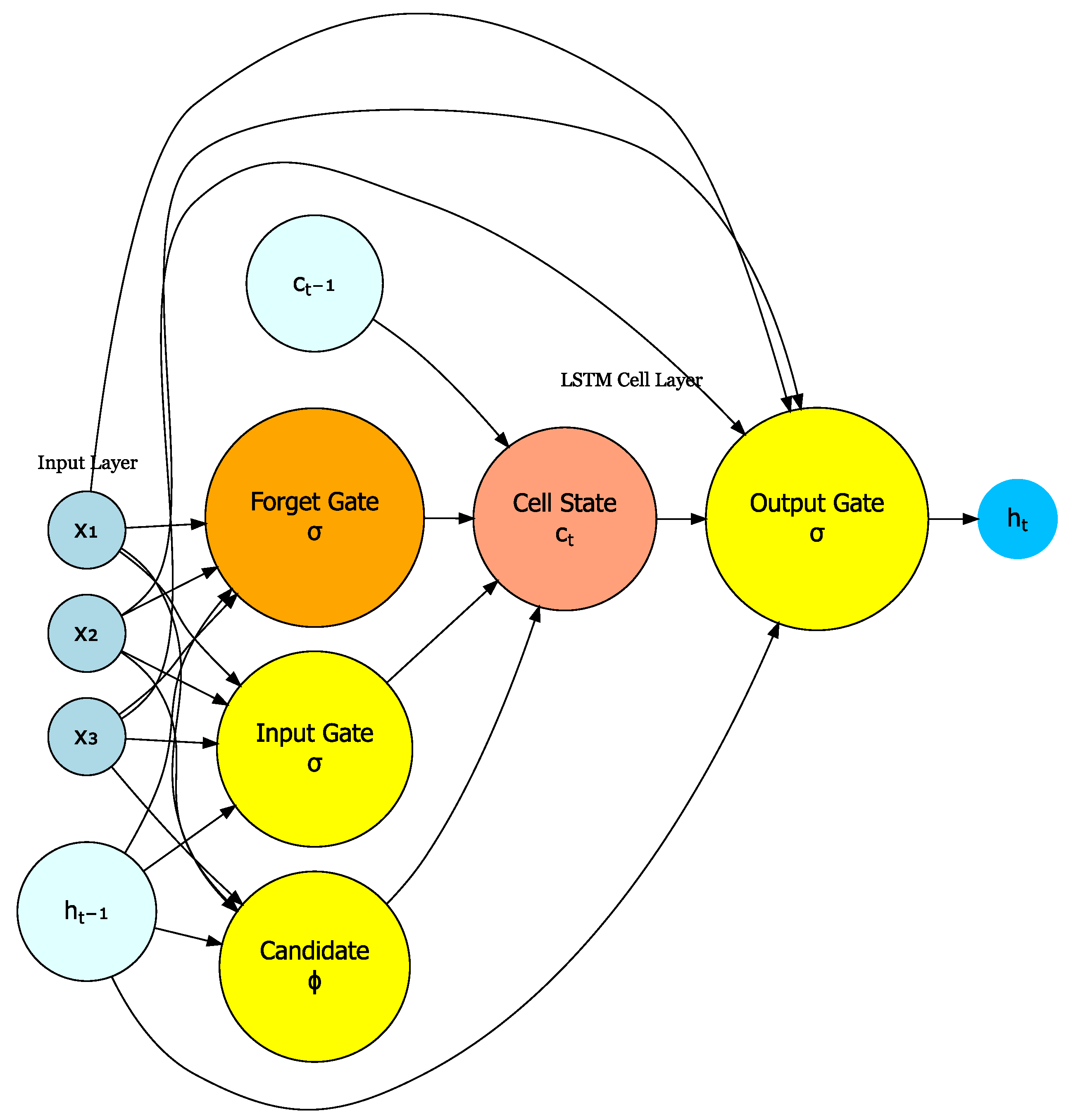
As illustrated in Figure 1, long-short-term memory networks are building blocks for the layers of a recurrent neural network (RNN). The LSTM connects the current neurons to the information from the prior data using the input gate, forget gate, and output gate found in each neuron, and this helps in resolving the issue of the data’s long-term reliance by utilising the input gate. Next, the internal gates of the LSTM architecture are outlined and explain how they address long-term dependency issues.

The Forget Gate: In Figure 1, the forget gate, which is defined in Equation (12) determines which information is to be discarded from the cell. This is done by entering the output $h_{t-1}$ at the previous unit $t-1$ and adding the current time t and input $r_t$ into a $sigmoid$ function $S_t$ that is defined in Equation (13). A value between 0 and 1 is generated, and this value is multiplied by the cell state $C_{t-1}$ to determine how much information is forgotten or remembered. The value 0 means completely forgotten, while 1 means completely remembered; hence, $\nu$ and $\zeta$ are the weight matrices and bias vector parameters, which need to be learned during training.

$$f_t=\sigma \left({\nu }_f·\left[h_{t-1},r_t\right]+{\zeta }_t\right)$$

(12)

$$S\left(t\right)={\displaystyle \frac{1}{1+exp-t}}$$

(13)

Input gate: In Figure 1, the input gate determines which new information is to be remembered in the cell state. By entering the output $h_{t-1}$ at the previous time $t-1$ and adding the current time t and an input $r_t$ to a $Sigmoid$ function defined in Equation (13), a value $i_t$ in Equation (14) is generated that is between 0 and 1 to decide how much new information in the cell state needs to be remembered. At the same time, a tanh function obtains an election message ${\tilde{C}}_t$ which is defined in Equation (15) to be added to the cell state by inputting the output $h_{t-1}$ at the previous time $t-1$ and adding the current time t and a piece of input of information $r_t$. Therefore, we multiply the values $i_t$ and ${\tilde{C}}_t$ just obtained by the $Sigmoid$ function to get the updated information that needs to be added to the cell state $C_t$ in Equation (16).

$$i_t=\sigma \left({\nu }_f·\left[h_{t-1},r_t\right]+{\zeta }_t\right)$$

(14)

$${\tilde{C}}_t=tanh\left({\nu }_c·\left[h_{t-1},r_t\right]+{\zeta }_c\right)$$

(15)

$$C_t=f_t\ast C_{t-1}+i_t\ast {\tilde{C}}_t$$

(16)

Output gate: In Figure 1, the output gate determines which information will be an output in the cell state. By entering the output $h_{t-1}$ at the previous point at time $t-1$, and adding the current time t and input $r_t$ into a $Sigmoid$ function, a value $i_t$ as shown in Equation (17) which is between 0 and 1, is generated to determine how many cell states leads to output. The cell state is first activated in the tanh function layer before being multiplied by $0_t$. The result of multiplication is the output information $h_t$ in Equation (18) of the LSTM block at time t.

$$0_t=\sigma \left({\nu }_f·\left[h_{t-1},r_t\right]+{\zeta }_t\right)$$

(17)

$$h_t=0_t\ast \tanh \left(C_t\right)$$

(18)

The LSTM architecture in this study consists of two layers with 64 hidden units each, ReLU and tanh activations, a dropout rate of 0.2, and a final dense layer for output. We train this architecture using the Adam optimiser with a learning rate of 0.001, a batch size of 32, and early stopping with a patience of 300 epochs. Feature inputs include temporal hierarchies (weekly to annual), macroeconomic indicators (e.g., inflation, interest rates, monetary policy), geopolitical events (e.g., COVID-19, Russia–Ukraine war), and market variables such as ZAR/BWP. The implementation is carried out using TensorFlow 2 of [19] in a Python 3.12 environment on high-performance computing infrastructure.

3.2. Transformer-Based Deep Learning Architecture

Conventional deep learning architectures, including RNNs, LSTMs, and gated recurrent units (GRUs), process sequences sequentially, which limits their efficiency on long inputs [20,21]. To overcome these challenges, this study adopts a Transformer-based deep learning architecture that leverages self-attention mechanisms to enable parallel sequence processing and capture long-range dependencies. Specifically, we apply a Transformer encoder to forecast the smoothed latent level of a univariate time series extracted using a state space Kalman filter, as detailed in Section 3.1.3. The model incorporates multiscale temporal features as in the LSTM, and takes a fixed-length input sequence of past observations and produces a point forecast for the subsequent time step in the training set.

Let $y_t$ denote the smoothed latent value at time t, from the state space Kalman filter from Section 3.1.3 and let $x_t\in {\Re }^d$ be a multiscale feature vector at the same time point, where $d=6$. The objective is to predict the future value $y_{t+1}$ using a window of the most recent L observations as

$$\{{\mathbf{x}}_{t-L},{\mathbf{x}}_{t-L+1},\dots ,{\mathbf{x}}_t\}\mapsto {\widehat{y}}_{t+1}.$$

(19)

Formally, Equation (19) seeks to approximate a function $f_{\theta }$ that is parameterised by $\theta$, such that

$${\widehat{y}}_{t+1}=f_{\theta }\left({\mathbf{x}}_{t-L:t}\right)$$

(20)

where the input encoding and positional representation for the multiscale input sequence $X\in {\Re }^{B\times L\times d}$, and B being the batch size, are then first projected into a higher-dimensional latent space as

$$H_0=X{W}_e+P.$$

(21)

In Equation (21), $W_e\in {\Re }^{d\times d_{\mathrm{model}}}$ is the embedding weight matrix, and $P\in {\Re }^{1\times L\times d_{\mathrm{model}}}$ is a learnable positional encoding tensor, which incorporates temporal order into the sequence. To incorporate transformer encoder layers, we pass the encoded sequence $H_0$ through multiple layers of a Transformer encoder. Each layer comprises a multi-head self-attention mechanism followed by a position-wise feedforward network. The self-attention operation is defined as

$$\mathrm{Attention}(Q,K,V)=\mathrm{softmax}\left({\displaystyle \frac{Q{K}^{\top }}{\sqrt{d_k}}}\right)V$$

(22)

where the query, key, and value matrices are computed as

$$Q=H{W}^Q,K=H{W}^K,V=H{W}^V$$

(23)

and $W^Q,W^K,W^V\in {\Re }^{d_{\mathrm{model}}\times d_k}$ are learnable parameter matrices. The output of the attention layer is normalised and passed through a feedforward layer with residual connections, that is given by

$$Z_1=\mathrm{LayerNorm}(H+\mathrm{Attention}\left(H\right))$$

(24)

and

$$H^{\prime }=\mathrm{LayerNorm}(Z_1+\mathrm{FFN}\left(Z_1\right)).$$

(25)

Nonetheless, the feedforward sublayer according to [22] is defined as

$$\mathrm{FFN}\left(z\right)=\mathrm{ReLU}(z{W}_1+b_1)W_2+b_2$$

(26)

where $W_1,W_2$ and $b_1,b_2$ are learnable weights and biases. To obtain the forecast, the representation corresponding to the final time step is extracted and passed through a linear output layer given by

$${\widehat{y}}_{t+1}=H^{\prime }[:,-1,:]W_o+b_o$$

(27)

where $W_o\in {\Re }^{d_{\mathrm{model}}\times 1}$ and $b_o\in \Re$ are the regression weights and bias, respectively.

3.3. Selection of Error Metrics for Assessment

The selection of suitable error metrics is essential for assessing the performance of forecasting models. Error metrics quantitatively measure prediction accuracy and evaluate the model’s ability to capture underlying data patterns. This study employs the following metrics.

• Mean Squared Error (MSE)

The MSE is a fundamental and widely used error metric in predictive modelling. It measures the average of the squared differences between the predicted values and the actual observations, thereby penalising larger errors more heavily. The mathematical formulation of MSE is

$$\mathrm{MSE}={\displaystyle \frac{1}{n}}\sum _{t=1}^n{(y_t-{\widehat{y}}_t)}^2$$

(28)

where n is the number of observations, $y_t$ is the actual value at time t, and ${\widehat{y}}_t$ is the predicted value at time t.

• Root Mean Squared Error (RMSE)

RMSE is the square root of MSE and presents the error in the same unit as the original data. It provides a more interpretable measure of the typical prediction error:

$$\mathrm{RMSE}=\sqrt{{\displaystyle \frac{1}{n}}\sum _{t=1}^n{(y_t-{\widehat{y}}_t)}^2}$$

(29)

This metric is especially useful when interpretability in the original scale is [23].

• Mean Absolute Error (MAE)

MAE represents the average absolute difference between predicted and actual values. Unlike MSE, it is less sensitive to outliers and provides a balanced measure of accuracy:

$$\mathrm{MAE}={\displaystyle \frac{1}{n}}\sum _{t=1}^n|y_t-{\widehat{y}}_t|$$

(30)

It is a robust metric for understanding overall model error without over-penalising large deviations [24].

• Mean Forecast Error (MFE)

MFE computes the average difference between forecasted and actual values without considering the direction of the error. It provides a sense of the average prediction deviation:

$$\mathrm{MFE}={\displaystyle \frac{1}{n}}\sum _{t=1}^n({\widehat{y}}_t-y_t)$$

(31)

While it does not account for directional bias (over- or under-forecasting), it is valuable for assessing the average magnitude of forecast errors [25].

3.4. Prediction Interval Evaluation Metrics

Prediction intervals (PIs) are central to probabilistic forecasting, representing a range within which the predicted value is expected to fall with a specified level of confidence. They communicate the inherent uncertainty of the forecasting model, which arises from data variability and the complexity of the system under study. Accurately constructed PIs are crucial for informed decision-making and effective risk management. In this study, we evaluate prediction intervals for both the LSTM and Transformer encoders using the Mean Prediction Interval Width (MPIW), which measures the average width of the constructed intervals. A narrower MPIW indicates greater predictive precision, provided that the intervals still maintain adequate coverage. The MPIW is defined by [26] as follows

$$\mathrm{MPIW}={\displaystyle \frac{1}{n}}\sum _{i=1}^n(U_i-L_i)$$

(32)

where n is the number of prediction intervals, $U_i$ is the upper bound of the $i\mathrm{th}$ interval, and $L_i$ is the lower bound. An effective prediction interval should achieve a high Prediction Interval Coverage Probability (PICP), ensuring the true values fall within the intervals, while also maintaining a narrow MPIW to preserve precision.

3.5. Risk Measures

Risk measures are historical indicators of investment risk and volatility that are necessary for modern portfolio theory (MPT). The MPT is a widely used commercial and academic approach for assessing a stock’s or fund’s performance against its benchmark index. This section looks at the recommended risk-management strategies for BWP/USD returns.

Maximum Drawdown

Maximum drawdown, which is the worst cumulative loss over a specific period, is one of the most widely used risk indicators in practice. Additionally, the definitions of the Sterling and Calmar ratios use maximum drawdown to evaluate the risk and performance of hedge funds and mutual funds. The following are some benefits of maximum drawdown over conditional VaR (CVaR) and value-at-risk (VaR). Refs. [7,27] have emphasised that it is more illuminating than VaR and CVaR, because it is easier to identify which asset has a lower maximum drawdown when two historical price charts are provided. Furthermore, it is simpler to determine the maximum drawdown directly from a time series since it is calculated from a straightforward sum of log returns during the drawdown period. Furthermore, the maximum drawdown is a risk metric that is independent of models and, as mentioned before, the maximum drawdown is the worst loss among successive declines from peaks to troughs during a given period. At time T, it is defined as

$$MDD=\underset{\tau \in \left(0,T\right)}{max}\left(\underset{t\in \left(0,T\right)}{max}\left(p\left(t\right)-p\left(\tau \right)\right)\right)$$

(33)

where $p\left(t\right)$ is the log price at time t. It can be expressed with log-returns

$$MDD=-\underset{\tau \in \left(0,T\right)}{min}\left(\underset{t\in \left(0,T\right)}{min}R\left(t,\tau \right)\right)$$

(34)

where $R\left(t,\tau \right)$ is the log-return between t and $\tau$. The maximum drawdown is regarded as the worst-case scenario for an investor who starts his/her investment in the period. It is obvious for investors to prefer smaller maximum drawdowns to larger drawdowns in portfolio performance.

3.6. Conditional Drawdown-at-Risk (CDaR)

Conditional Drawdown-at-Risk is a coherent risk measure that quantifies the expected drawdown of an asset, conditional on the drawdown exceeding a given quantile threshold. Unlike Value-at-Risk (VaR), which considers only terminal losses, CDaR incorporates the temporal dimension of losses, making it particularly suitable for evaluating downside risk in sequential return data. The CDaR at confidence level $\alpha$ is defined as the average of the worst drawdowns that exceed the drawdown-at-risk (DaR) at level $\alpha$.

Let $D\left(t\right)$ denote the drawdown at time t, which is defined as the decline from the historical peak as

$$D\left(t\right)=M\left(t\right)-X\left(t\right),$$

(35)

where $X\left(t\right)$ is the portfolio value at time t, and $M\left(t\right)={max}_{s\le t}X\left(s\right)$ is the historical running maximum. The Drawdown-at-Risk (DaR) at level $\alpha$ is now given by

$${\mathrm{DaR}}_{\alpha }=inf\left\{d\in \Re :\mathbb{P}(D>d)\le 1-\alpha \right\}.$$

(36)

Taking the expectation of the drawdowns exceeding DaR in Equation (36), we can compute the CDaR as the

$${\mathrm{CDaR}}_{\alpha }=\mathrm{E}[D\left(t\right)\mid D\left(t\right)>{\mathrm{DaR}}_{\alpha }].$$

(37)

3.7. Downside Deviation

Downside deviation is a measure of volatility that captures the variability of returns falling below a minimum acceptable return (MAR), typically the risk-free rate or zero. Unlike the standard deviation, which penalises both upside and downside variability, downside deviation focuses solely on the negative tail, aligning more accurately with investors’ risk perceptions. Now, let $R_t$ be the return at time t and T the total number of observations. The downside deviation is computed by

$${\sigma }_d=\sqrt{{\displaystyle \frac{1}{T}}\sum _{t=1}^{T}min{(R_t-\mathrm{MAR},0)}^2}.$$

(38)

This measure enables the calculation of downside risk-adjusted performance ratios, such as the Sortino Ratio, and is more relevant in risk-sensitive performance evaluation, particularly in turbulent market conditions such as the exchange rate market.

3.8. Backtesting Risk Measures

Backtesting techniques evaluate the forecast’s adequacy when a set of VaR forecasts is available. Procedures for value-at-risk backtesting often verify that the unconditional and conditional left-tail of the log-returns distribution is correctly covered. Backtesting is a statistical method used to compare actual losses with appropriate risk measures, with exceptions occurring once every 100 days with a 99% confidence level. This process evaluates whether the frequency of these exceptions aligns with the specified confidence level [28]. These tests, known as binding tests, are relatively easy to implement if no exceptions occur [29], and common methods for backtesting risk models include the Kupiec likelihood ratio (LR) test for unconditional coverage by [30], the Christoffersen test for conditional coverage, which extends the Kupiec test [31], and the Basel III green zone, updated by [32]. But, in this study, the focus is based on the Kupiec, Christoffersen test, quantile Loss Function (Pinball Loss) and concordance correlation coefficient (CCC).

Christoffersen Likelihood Ratio

This test, known as the Markov test, checks for the independence property by analysing whether the probability of a VaR violation on a given day is influenced by the outcome of the previous day. It helps to evaluate both the unconditional distribution of returns and the volatility clustering often observed in financial time series. Additionally, time-varying volatility in financial markets is accounted for by this test, and it is crucial for accurately capturing the evolving nature of risk. By defining $p_{ij}={\displaystyle \frac{{\eta }_{ij}}{{\sum }_j{\eta }_{ij}}}$ where $p_{ij}$ presents a violation probability that occurs conditionally on state i at a time $t-1$ such that $p_1={\displaystyle \frac{{\eta }_{11}}{{\eta }_{11}+{\eta }_{21}}}$, $p_2={\displaystyle \frac{{\eta }_{22}}{{\eta }_{12}+{\eta }_{22}}}$ and $p={\displaystyle \frac{{\eta }_{11}+{\eta }_{22}}{N}}$, then the Christoffersen likelihood ratio test statistic is given by

$$L{R}_{cC}=-2ln\left({\displaystyle \frac{\left(1-p\right){\eta }_{11}+{\eta }_{12}+p{\eta }_{21}+{\eta }_{22}}{\left(1-p\right){\eta }_{11}{p}_1{\eta }_{21}\left(1-p_2\right){\eta }_{12}{p}_2{\eta }_{22}}}\right).$$

(39)

In line with [33], Equation (39) is an asymptotic chi-square distribution with one degree of freedom, and it is computed using

$${\chi }^2=\sum _{k=1}^n{\displaystyle \frac{{(O_k-E_k)}^2}{E_k}}$$

(40)

$O_k$ is the set of observed counts, and $E_k$ is the expected counts under the null hypothesis. Reject the null hypothesis if the calculated probability value is less than the observed one.

3.9. Quantile Loss Function (Pinball Loss)

The Quantile Loss function, also known as the Pinball Loss, evaluates the accuracy of quantile forecasts at a given quantile level $\tau \in (0,1)$. It penalises over-predictions and under-predictions asymmetrically to better capture risk at the desired quantile. The Quantile Loss over T observations is defined as

$${\mathrm{QL}}_{\tau }(y_t,{\widehat{q}}_t\left(\tau \right))=\sum _{t=1}^T{\rho }_{\tau }\left(y_t-{\widehat{q}}_t\left(\tau \right)\right),$$

(41)

where the check function ${\rho }_{\tau }\left(u\right)$ is given by

$${\rho }_{\tau }\left(u\right)=\left\{\begin{array}{cc}\tau u,\hfill & \mathrm{if}u\ge 0,\hfill \\ (\tau -1)u,\hfill & \mathrm{if}u<0.\hfill \end{array}\right.$$

(42)

Minimising ${\mathrm{QL}}_{\tau }$ in Equation (42) corresponds to improved accuracy in forecasting the $\tau$-quantile, such as Conditional Drawdown-at-Risk (CDaR).

3.10. Concordance Correlation Coefficient (CCC)

The Concordance Correlation Coefficient, on the other hand, measures the agreement between observed values $X=\{x_1,\dots ,x_T\}$ and predicted values $Y=\{y_1,\dots ,y_T\}$, combining precision and accuracy into a single metric. It is defined as

$${\rho }_c={\displaystyle \frac{2\rho {\sigma }_X{\sigma }_Y}{{\sigma }_X^2+{\sigma }_Y^2+{({\mu }_X-{\mu }_Y)}^2}},$$

(43)

where $\rho$ is the Pearson correlation coefficient between X and Y, ${\sigma }_X^2$ and ${\sigma }_Y^2$ are the variances of X and Y, respectively, and ${\mu }_X$ and ${\mu }_Y$ are the means of X and Y, respectively. The value of ${\rho }_c$ ranges from $-1$ to 1, with values closer to 1 indicating strong concordance between observed and predicted values. This makes it a robust metric for evaluating the performance of risk forecasts such as Maximum Drawdown, CDaR, and Downside Deviation.

4. Results

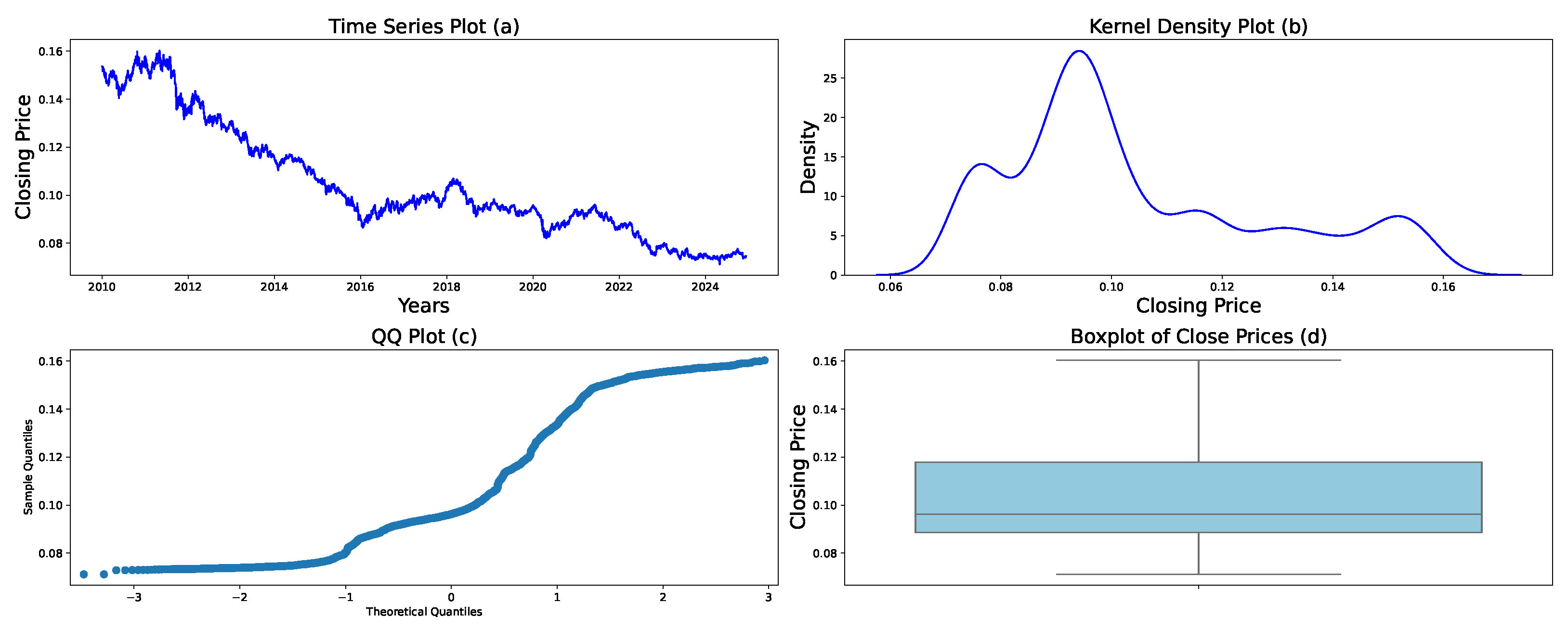
This section describes an empirical analysis of the study using time series data of BWP/USD from 2 January 2010 to 31 May 2025. This data is obtained from https://finance.yahoo.com/ (accessed on 1 June 2025, using the Yahoo Finance package from Python). This makes a total of 3978 observations. Training and testing sets are the two categories into which the data is divided. Univariate data analysis for the variables of interest—the BWP/USD returns are shown in Figure 2. We use the returns series to assess the stylised facts of the BWP/USd exchage rate and also use them to compute the downside risk. Panel (a) demonstrates a consistent downward trend in the time series, reflecting a gradual depreciation in BWP/USD value from 2010 to 2025, likely influenced by unfavourable macroeconomic conditions or inherent market weaknesses. Panel (b) presents the kernel density plot, which indicates a left-skewed distribution characterised by a significant peak at approximately 0.095. This suggests that the majority of values are concentrated around this level, while the extended tail signifies occasional low-price occurrences. Panel (c), the Q–Q plot, indicates notable deviations from normality, especially in the distribution’s tails, suggesting the existence of heavy-tailed behaviour or non-Gaussian characteristics frequently found in financial data. Finally, panel (d), the box-and-whisker plot, indicates moderate variability, with a median near 0.10 and an interquartile range roughly between 0.09 and 0.12. The extended lower whisker supports the identified negative skewness, while the existence of outliers highlights the irregular and extreme variations in closing prices. The plots indicate that standard linear models such as seasonal autoregressive integrated moving average (SRAIMA) based on normality assumptions may be insufficient, suggesting the need for more robust or non-parametric methods for accurate modelling and inference.

The observed movements in the BWP/USD exchange rate, particularly the sustained depreciation and volatility, can be attributed to a combination of macroeconomic and structural factors. Botswana’s persistent trade imbalances, driven by a heavy reliance on imports relative to export earnings, exert downward pressure on the Pula. Additionally, the country’s dependence on diamond exports exposes the exchange rate to global commodity price fluctuations. Monetary policy differentials between the Bank of Botswana and the US Federal Reserve can also influence capital flows, with higher US interest rates attracting investment away from the Pula. Inflation differentials, whereby domestic inflation outpaces that of the US, further erode the Pula’s real value. External shocks such as the COVID-19 pandemic, coupled with global risk aversion, tend to favour safe-haven currencies like the US Dollar. Moreover, Botswana’s crawling peg exchange rate regime allows for a managed depreciation over time. Investor sentiment and speculative activity, often influenced by political or economic uncertainty, may further contribute to the currency’s volatility and long-term decline. Recently, ref. [34] declared that the current economic environment is characterised by several key factors, including: (1) subdued economic performance, as indicated by GDP contraction in both 2024 and 2025; (2) a sharp decline in mining (diamond) output and low growth rates in the non-mining sector, underscoring a continued reliance on mining for overall economic growth and a general lack of diversification and productivity in other sectors; (3) significant decrease in the official foreign exchange reserves, mainly due to lower export earnings, while the demand for imports remains high; and (4) apart from the official foreign exchange reserves, commercial banks and other entities hold a considerable amount of foreign currency.

The results of the Jarque–Bera test in

Table 1. Descriptive Statistics of BWP/USD Returns.

	Mean	Skewness	Kurtosis
BWP/USD Returns	−0.000165	−0.07218	6.48467
Test	Statistics		p-value
Jarque–Bera	6820.905		0.001
Ljung–Box	34.587		0.001
ARCH LM Test	558.686		0.001

at the level of significance 5%, which reject the null hypothesis of normality, imply that symmetric models are not appropriate to evaluate the BWP/USD returns. The results of the Ljung–Box test for BWP returns indicate an insignificant p-value, which suggests that the returns are taken to be independently and identically distributed and does not rule out the null hypothesis of no autocorrelation. The ARCH test rejects the null hypothesis, indicating that the BWP/USD returns possess volatility clustering, allowing the estimation of the state space Kalman filter to mitigate this clustering volatility before the training of the LSTM and the Transformer encoder.

4.1. De-Noising a Time Series with a State Space Kalman Filter

To denoise the BWP/USD, we fit the unobserved components model that follows a local level specification, and the final estimated model is given in

Table 2. Maximum likelihood estimates from the local level model.

Parameter	Coef	Std. Err	z	P > z	[0.025]	[0.975]
${\sigma }_{\mathrm{irregular}}^2$	0.00000009728	0.00000000389	24.984	0.000	0.0000000896	0.000000105
${\sigma }_{\mathrm{level}}^2$	0.0000003178	0.00000000824	38.570	0.000	0.000000302	0.000000334

.

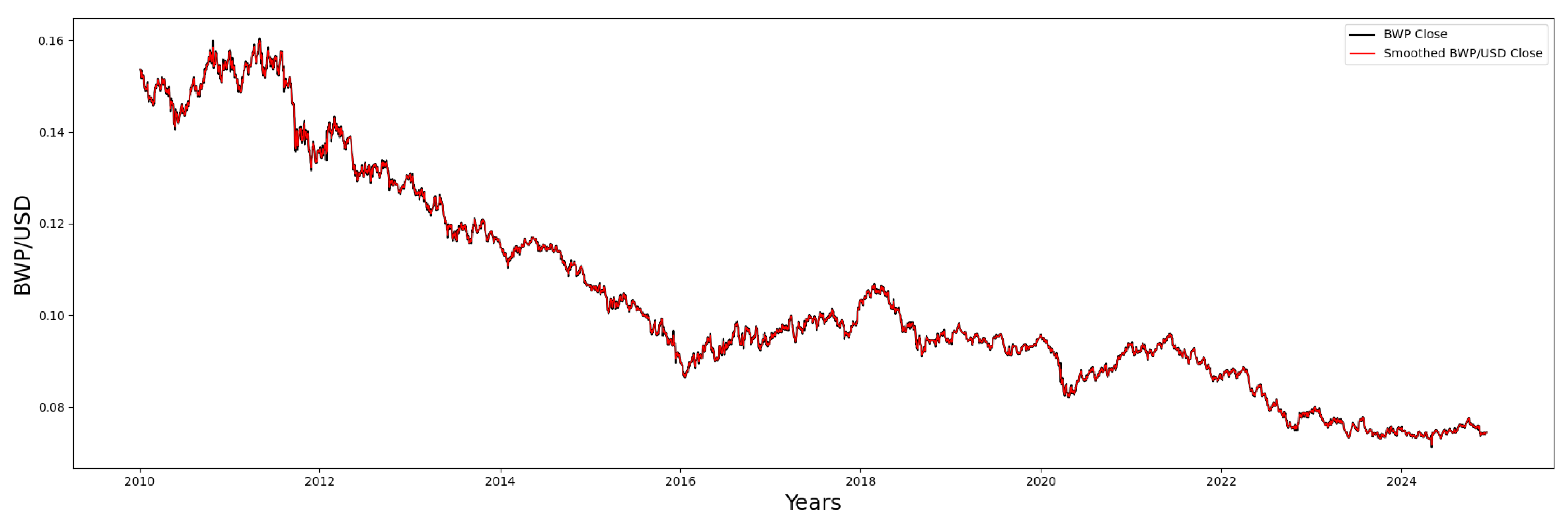
The estimated variance of the irregular component, ${\sigma }_{\mathrm{irregular}}^2$, is exceptionally small, indicating that the observed values remain closely aligned with the estimated underlying level. In contrast, the variance of the level of innovation, ${\sigma }_{\mathrm{level}}^2$, is notably larger, suggesting that the latent level evolves with greater flexibility over time. The disparity in the magnitude of these variances implies that the BWP/USD closing prices are predominantly influenced by a gradually changing trend, rather than by transient fluctuations. The statistical significance of both variance estimates is substantiated by substantial z-statistics—24.984 and 38.570, respectively—and highly significant p-values (both less than 0.001). These results provide compelling evidence that the model’s level and irregular components are both integral to accurately capturing the dynamics of the BWP/USD closing prices, and these results are also confirmed by Figure 3.

4.2. Short, Medium, and Long-Term Forecasting

A collection of temporal hierarchies, ranging from day to yearly frequencies, is generated using the residuals obtained from the fitted state space Kalman filter model. Alongside these endogenous characteristics, many external factors are used to improve the forecasting model. This encompasses sentiment indices pertinent to Botswana’s monetary policy, geopolitical tensions arising from the Russia–Ukraine conflict, information regarding the 2015/2016 Shanghai stock market crash, Botswana’s daily confirmed COVID-19 cases, and macroeconomic indicators including Botswana’s interest rate, inflation rate, and the exchange rate of the South African rand against the Botswana pula. These properties together function as inputs to a Long-Short-Term Memory (LSTM) network, which is specially designed to capture temporal dynamics and nonlinear correlations in financial time series data. The LSTM architecture consists of one LSTM layer, followed by a Dropout layer to mitigate overfitting, and two fully connected Dense layers. The Transformer architecture includes a linear input projection layer that transforms the raw time series into a higher-dimensional feature space, augmented with learnable positional encodings to maintain the temporal structure. The representation undergoes processing through a series of Transformer Encoder layers. Each layer consists of multi-head self-attention mechanisms and position-wise feedforward networks, with dropout techniques implemented to reduce the risk of overfitting. The most recent time step’s final hidden state is extracted and forwarded through a fully connected output layer to generate the forecast. Both the LSTM and the Transformer architectures are structured to manage forecasting tasks over various time horizons: short-term (5 days), medium-term (30 to 90 days), and long-term (180 to 240 days). They both enable a thorough assessment of exchange rate risk and temporal dependencies that are pertinent to trading strategies and monetary policy analysis.

The LSTM model shows remarkable in-sample performance with a Root Mean Squared Error (RMSE) of 0.00075, a Mean Absolute Error (MAE) of 0.00062, and a Mean Squared Error (MSE) of almost zero, all of which indicate a perfect fit to the training data as reported in

Table 3. LSTM model performance.

	MSE	MAE	MFE	RMSE
In-sample	0.00000	0.00062	0.00057	0.00075
Out-of-sample
7 days	0.00002	0.00394	0.00394	0.00394
30 days	0.00002	0.00400	0.00400	0.00401
90 days	0.00001	0.00288	0.00288	0.00309
180 days	0.00001	0.00219	0.00219	0.00230
240 days	0.00002	0.00177	0.00177	0.00190

. The Mean Forecast Error (MFE = 0.00057) provides additional evidence that the model’s in-sample forecasts are not biased. Especially over the short and medium term, the model’s out-of-sample findings show that it maintains a high level of prediction accuracy. To illustrate the point, the RMSE for the 7-day prediction is 0.00394, but the RMSE for the 30-day and 90-day horizons are 0.00401 and 0.00309, respectively, indicating steady and somewhat better error metrics. Longer time horizons show an approximate rise in error, with RMSE reaching 0.00330 at 180 days and 0.00390 at 240 days, although these numbers are still within acceptable ranges for predicting. There seems to be no consistent over- or under-prediction, since MAE and MFE are quite near to each other over all forecast periods. The model’s strong generalisability makes it useful for predicting the behaviour of BWP/USD exchange rates across a range of investment- and policy-relevant time horizons.

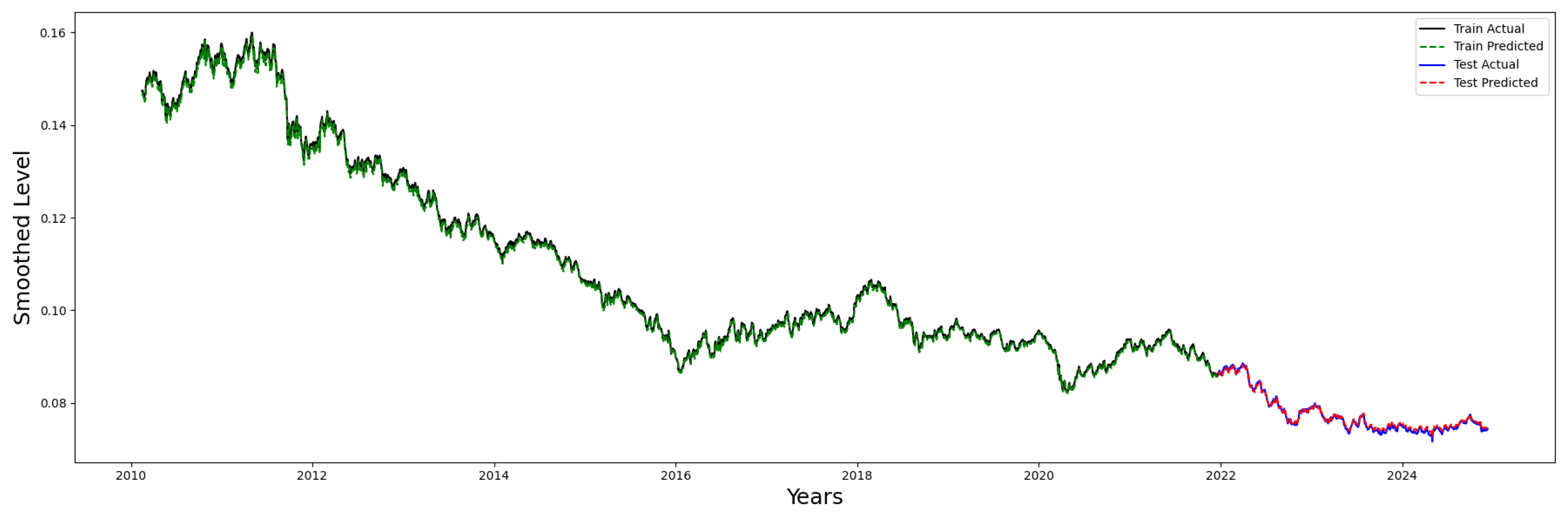
As visually inspected in Figure 4, during the training phase, which begins in 2010 and ends in late 2021, the actual and the predicted (forecasted) are closely aligned. This shows that the LSTM model has learnt trends and patterns in the historical data, which fits the training set well. The actual and the predicted in the training set show that the LSTM mimics the training data, indicating that there is very little residual error. For the testing procedure, both the predicted and actual values are close to each other, indicating a good modelling of the LSTM that mimics the BWP/USD exchange rates. This illustrates the actual and predicted values for the future, respectively. The LSTM architecture seems to have caught the general trend of decreasing test data at this stage. Although the model generally follows the blue solid line, the red dashed line often exaggerates or understates the actual values, particularly as the series continues to decline. Transitioning from in-sample to out-of-sample prediction is characterised by bigger prediction errors than training. This seems to be the case here. Because of the test set’s finer details and smaller oscillations, the model has difficulty accurately reproducing them.

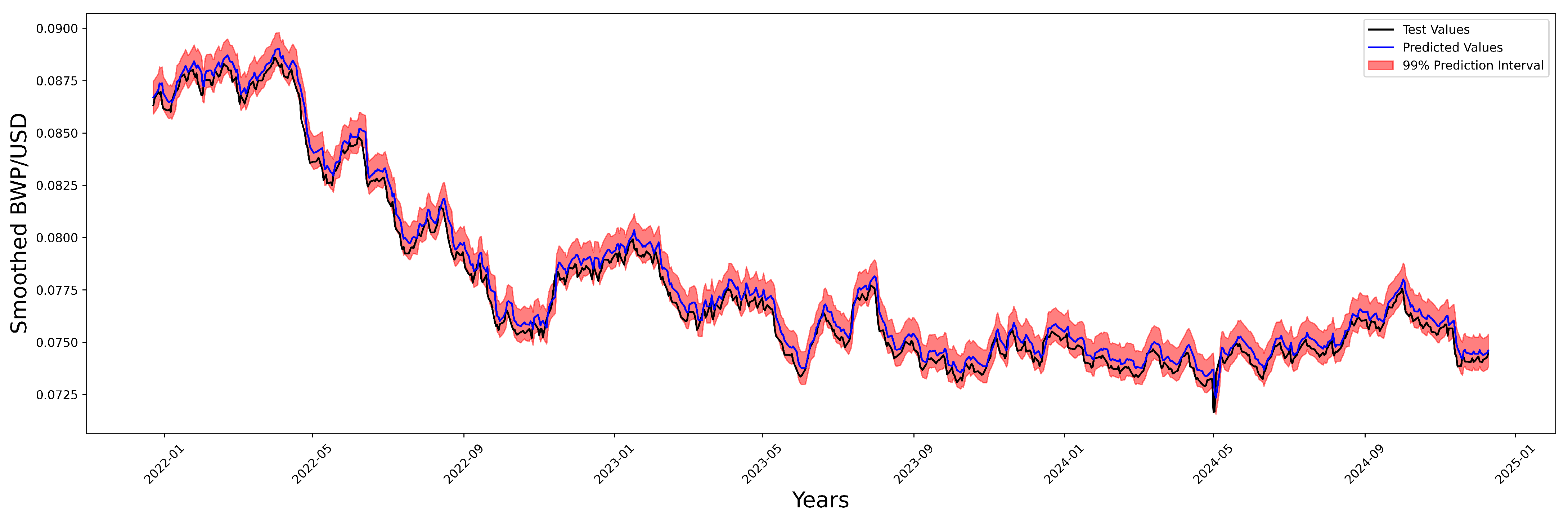
Assessing the stability of the LSTM model is essential for determining its ability to accurately predict the “Smoothed BWP/USD” exchange rate and to evaluate whether it effectively represents the actual range of future values. The model exhibits a Mean Prediction Interval Width (MPIW) of 0.0016, and the 99% prediction interval is illustrated in the accompanying Figure 5, which provides significant insights into its predictive reliability and the related forecast uncertainty. The narrow MPIW of 0.0016 indicates that the LSTM model attains high forecast precision, despite the inherent volatility present in the BWP/USD exchange rate. This holds particular significance in economic and financial contexts, where minor deviations can lead to substantial consequences. The visual analysis of the figure reveals that the actual “Smoothed BWP/USD” test values (depicted in black) predominantly, if not entirely, reside within the 99% confidence band (illustrated as a pink shaded area). This close alignment enhances the model’s ability to accurately represent the distributional characteristics of the exchange rate, encompassing both its central tendency and variability. The LSTM’s ability to produce stable and consistent out-of-sample forecasts, along with effective uncertainty quantification, underscores its suitability for economic and financial applications. This is especially relevant in situations where dependable forecasts of currency fluctuations and precise evaluations of related risks are crucial for informed decision-making and risk management approaches.

The Transformer model has a moderate degree of accuracy in the sample, with an MSE of 0.00567, an MAE of 0.06894, and an RMSE of 0.07529 as seen in

Table 4. Transformer Model Perfomance.

Forecast Horizon	MSE	MAE	MFE	RMSE
In-Sample	0.00567	0.06894	0.06894	0.07529
Out-of-Sample
7 days	0.00002	0.00399	0.00399	0.00400
30 days	0.00001	0.00362	0.00362	0.00370
90 days	0.00001	0.00276	0.00276	0.00290
180 days	0.00001	0.00344	0.00344	0.00359
240 days	0.00001	0.00363	0.00363	0.00376

. This result shows that it fits the training data well, although it has somewhat more errors than the LSTM model. The in-sample Mean Forecast Error (MFE = 0.06894) shows that the model’s training forecasts have a slight upward bias. However, projections made outside of the sample show a lot of progress and stability across different time-frames. The RMSE is very low for short-term forecasts (7 days), at 0.00400, and for 30-day predictions, at 0.00370. This result shows that the model is good at catching changes that will happen soon. The RMSE values for medium- to long-term projections (90, 180, and 240 days) are 0.00290, 0.00359, and 0.00376, which show that the forecasts are still accurate. The fact that MAE and MFE are in line with each other across all forecast horizons shows that the model does not have a systematic bias in its predictions. Overall, the Transformer model is a satisfactory way to describe changes in exchange rates over both short and long periods of time, even if it has a greater in-sample error. It has strong generalisation capacity and steady forecasting accuracy.

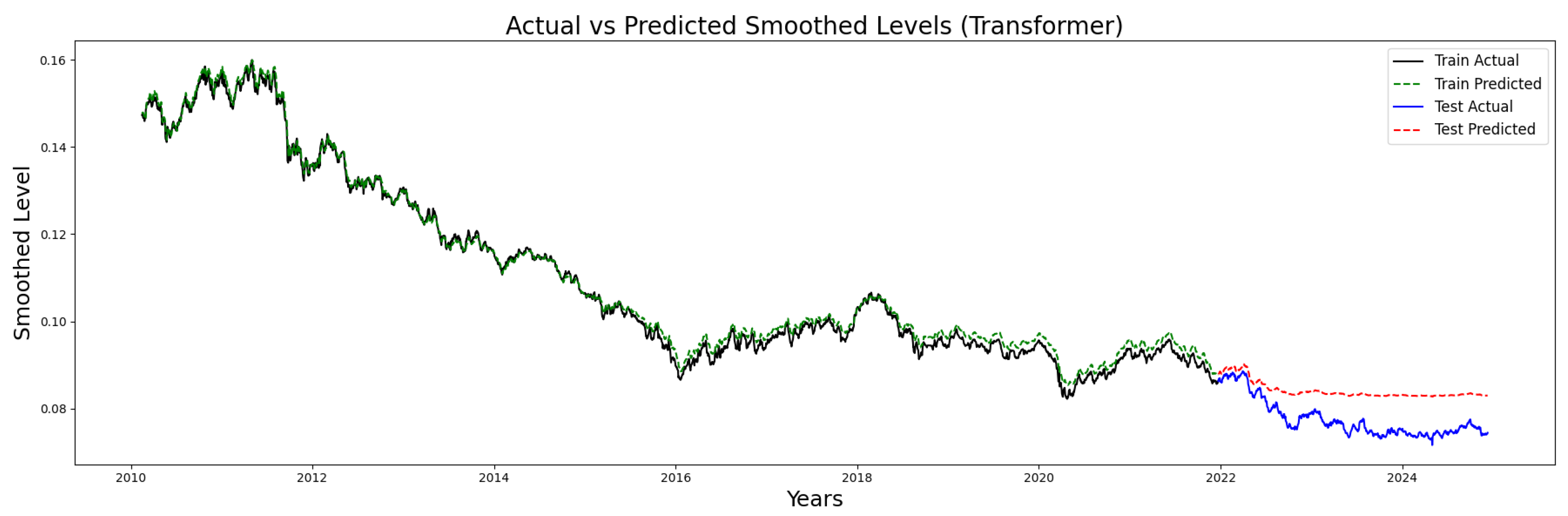
Figure 6, illustrates the performance of the Transformer model in forecasting BWP/USD closing prices. During the training phase (circa 2010 to late 2021), the Transformer demonstrates excellent fit, with the “Train Actual” closely aligned with the “Train Predicted”, indicating that the model effectively captures complex temporal dependencies in historical data. However, in the testing phase (late 2021 to early 2025), a noticeable divergence emerges. While the Transformer initially tracks the downward trend, its predictions (red dashed line) begin to deviate from the actual trajectory, particularly during the sharper declines of 2022 and 2023. This suggests that the model tends to overly smooth future values, underestimating volatility and failing to respond adequately to rapid changes. Moreover, toward the end of the forecast horizon (2024–2025), the model consistently overpredicts, indicating a persistent positive bias and reduced adaptability to continued downward trends.

The comparative evaluation of the LSTM and Transformer architectures reveals that the LSTM consistently outperforms the Transformer across all in-sample and out-of-sample forecasting horizons. In-sample, the LSTM achieves near-zero error metrics (MSE = 0.00000, MAE = 0.00062, RMSE = 0.00075), indicating an excellent fit to the training data. Out-of-sample, the LSTM maintains superior accuracy, particularly over longer horizons, with the lowest RMSE of 0.00190 for the 240-day forecast. In contrast, while the Transformer architecture performs comparably in short-term forecasting (e.g., 7-day RMSE = 0.00400), it exhibits significantly higher in-sample errors (MSE = 0.00567, MAE = 0.06894), suggesting overparameterisation or underfitting. Over extended horizons, the Transformer shows increased forecast errors, such as an RMSE of 0.00376 at 240 days, nearly double that of the LSTM. These results suggest that the LSTM model offers a more robust and reliable approach for both short- and long-term time series forecasting in this context. Moreover,

Table 5. Comparative Summary of LSTM and Transformer Performance on BWP/USD Exchange Rate.

Capability	LSTM	Transformer	Best Performer
Short-Term	lowest RMSE and MAE	Slightly higher error	LSTM
Medium-Term	Strong accuracy	Increase in error	LSTM
Long-Term	Robust long-range fit	Higher errors	LSTM
In-Sample Fit	Near-perfect fit	Higher errors	LSTM
Feature	Effective	Captures complex patterns	LSTM
Overall	Superior performance	Higher forecasting error	LSTM

demonstrates the superiority of the LSTM over the Transformer. Across specific capabilities, the LSTM consistently delivers stronger performance: it achieves the lowest short-term error metrics, maintains robust accuracy in medium- and long-term horizons, and provides a near-perfect in-sample fit. Although the Transformer demonstrates some strength in capturing complex patterns, this advantage does not translate into lower forecast errors. Overall, the LSTM emerges as the best-performing model, offering a more robust and reliable approach for short-, medium-, and long-term forecasting of the BWP/USD exchange rate.

4.3. Feature Importance and Forecasting of Downside Risk

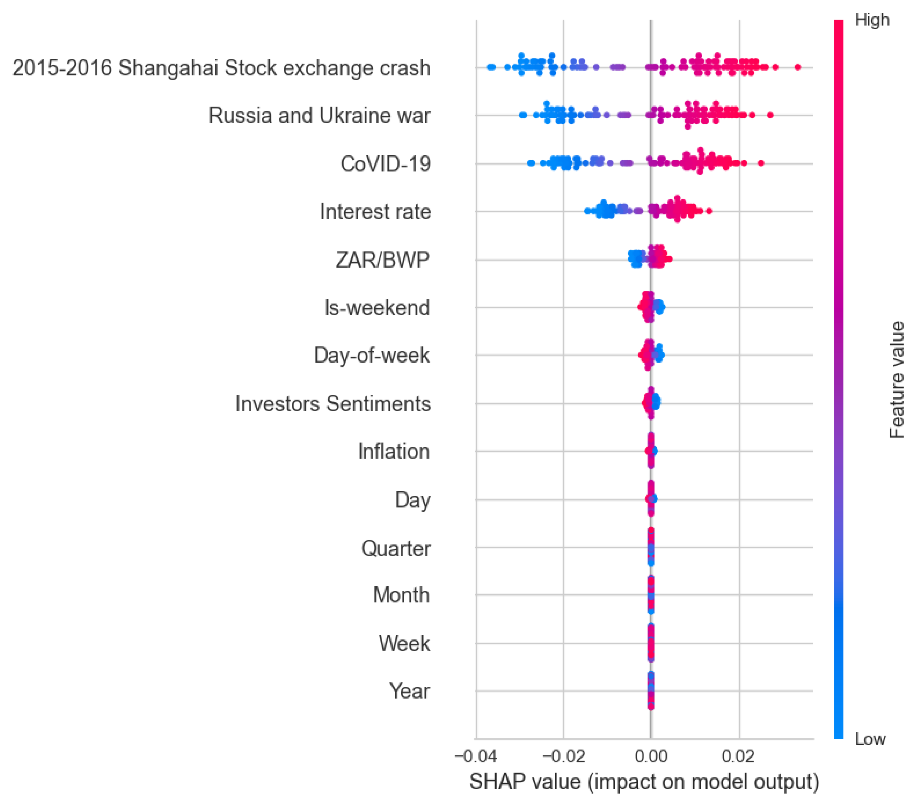
The SHAP (SHapley Additive exPlanations) analysis, as reported in Figure 7, offers critical insight into the relative importance and directional influence of features within the state space Kalman filter–LSTM forecasting model for the BWP/USD exchange rate. According to [35], these features help to accurately assess the downside risk by identifying the most influential features of the model. The most impactful predictors include major historical and geopolitical events—namely the 2015–2016 Shanghai Stock Exchange crash, the Russia–Ukraine war, and the COVID-19 pandemic—whose presence consistently pushes the model’s predictions upward, as indicated by positive SHAP values associated with high feature values. In contrast, the absence of these events corresponds with negative SHAP values, reflecting downward pressure on exchange rate forecasts. Economic indicators such as the interest rate and the ZAR/BWP exchange rate also exhibit considerable influence. While high interest rates tend to increase the model’s output, their effect is less uniform, suggesting complex interactions with other macroeconomic variables. The ZAR/BWP exchange rate shows a clear positive correlation, with higher values contributing to increased model predictions, emphasising the regional interdependence between Botswana and South Africa’s currency movements. In contrast, temporal features—such as inflation, year, quarter, month, week, and day—exhibit minimal explanatory power, as evidenced by SHAP values concentrated around zero, indicating a negligible impact on model output. Collectively, the SHAP results reinforce the conclusion that the model’s predictive accuracy is driven predominantly by structural macroeconomic shocks and regional exchange rate dynamics, rather than seasonal or cyclical calendar effects.

For the downside risk,

Table 6. Performance Metrics Across Different Forecast Horizons.

Horizon (Days)	Actual MDD	Predicted MDD	Actual CDaR (95%)	Predicted CDaR (95%)	Actual Downside Deviation	Predicted Downside Deviation
7	0.0011	0.0015	0.0011	0.0013	0.000303	0.000299
30	0.0234	0.0231	0.0230	0.0234	0.001816	0.001570
90	0.0410	0.0414	0.0393	0.0388	0.001415	0.001420
180	0.0410	0.0414	0.0385	0.0389	0.001420	0.001417
240	0.0581	0.0585	0.0503	0.0501	0.001501	0.001499

provides a comparative analysis of actual and predicted values for three primary downside risk metrics: Maximum Drawdown (MDD), Conditional Drawdown-at-Risk (CDaR at 95%), and Downside Deviation, across multiple forecast horizons of 7, 30, 90, 180, and 240 days. The results show that the forecasting model exhibits high accuracy and consistency, with predicted values closely matching actual outcomes across all horizons and risk measures. The model demonstrates no systematic bias, as it does not consistently overestimate or underestimate the risk metrics. The observed marginal differences between actual and predicted values are within acceptable tolerance thresholds, indicating that the model is well calibrated and effectively captures the underlying distributional properties of the analysed financial time series. This alignment across short- and long-term horizons indicates that the model demonstrates strong generalisation capabilities and robustness to variations in time scale. The close alignment noted in the downside deviation estimates further supports the model’s reliability in evaluating tail risk. The findings demonstrate the model’s effectiveness for practical risk forecasting and management, especially in scenarios requiring precise estimation of downside risk.

The SHAP analysis distinctly illustrates Botswana’s structural susceptibility to global systemic shocks. Significant international occurrences, including the Russia–Ukraine war, the COVID-19 pandemic, and the Shanghai Stock Exchange crash, serve as primary factors contributing to downside risk in the BWP/USD exchange rate. In light of the application of SHAP, ref. [36] evaluated the raw materials interactions of steel-fibre-reinforced concrete using SHAP. However, our findings in this study highlight Botswana’s vulnerability to external shocks, despite being a relatively small, resource-based economy. The implication is that Botswana’s macroeconomic policy structure must adopt a more adaptive and proactive approach, integrating early-warning systems to monitor geopolitical tensions and global financial fluctuations. The significant positive SHAP influence of the ZAR/BWP exchange rate indicates a high level of regional currency interdependence. South Africa, as Botswana’s primary trading partner, significantly influences Botswana’s exchange rate dynamics through various shocks [37], including changes in interest rates, inflationary trends, and political events. The interdependence indicates that the Bank of Botswana’s monetary policy must be formulated in conjunction with regional financial institutions and necessitates the strategic development of hedging mechanisms to address ZAR-linked volatility.

The weak influence of temporal features, including month, quarter, or week, indicates that downside risk in the BWP/USD exchange rate is not driven by seasonal factors. This restricts the efficacy of conventional calendar-based macroeconomic interventions and highlights the need for event-driven policy responses, including adaptable fiscal rules, contingency reserves, or intervention mechanisms activated by external economic indicators. The Kalman filter–LSTM architecture demonstrates a capacity for generating stable and precise forecasts of Maximum Drawdown, Conditional Drawdown at Risk, and downside deviation, thereby affirming its relevance in forward-looking risk management. Financial institutions, such as banks and pension funds, may employ these forecasts for stress testing and optimal capital allocation. Government agencies can use them to plan foreign exchange reserves in anticipation of unfavourable currency fluctuations. Furthermore, companies involved in international trade may utilise these insights to mitigate foreign exchange risks, thus improving operational resilience. The institutionalisation of forecasting models within the national financial oversight framework could improve Botswana’s credibility with international investors and credit rating agencies. Proactive mitigation of downside risks via model-informed policy responses can reduce vulnerability to currency crises and enhance sovereign risk assessments, leading to lower external borrowing costs.

4.4. Backtesting Downside Risk Measures

The outcomes of backtesting the predicted risk measures from the LSTM model across various forecast horizons are presented in

Table 7. Backtesting Results of Predicted Risk Measures.

Horizon (Days)	Violations (CDaR)	Kupiec Test (p-Value)	Christoffersen Test (p-Value)	Violations (MDD)	Downside Deviation Bias (%)
7	1/30	0.673	0.812	0/30	1.32%
30	2/30	0.498	0.619	1/30	1.56%
90	2/30	0.392	0.731	1/30	0.35%
180	3/30	0.220	0.665	2/30	0.21%
240	4/30	0.135	0.543	2/30	0.13%

. The table presents the counts of violations for Conditional Drawdown at Risk (CDaR) and Maximum Drawdown (MDD), as well as p-values derived from the Kupiec unconditional coverage and Christoffersen independence tests. In the shortest range of 7 days, the model demonstrates 1 CDaR violation out of 30 instances and no MDD violations, with p-values of 0.673 and 0.812, respectively. This suggests that the model’s predictions are statistically well calibrated. With a forecast horizon of 240 days, the count of CDaR violations rises slightly to four, accompanied by Kupiec and Christoffersen p-values of 0.135 and 0.543, which remain above typical significance thresholds and therefore do not indicate a rejection of model adequacy. The downside deviation bias is consistently low across all time horizons, beginning at 1.3% for 7 days and decreasing to 0.13% at the 240-day horizon. This indicates that the LSTM model does not significantly overestimate or underestimate downside risk and is effective in capturing long-term drawdown dynamics.

4.5. Discussion of Results

This study uses a methodology that combines a local-level state space model with deep learning techniques to denoise and predict the BWP/USD exchange rate series. The Kalman filter, based on the premise of normally distributed disturbances, efficiently isolates the smoothed level of the series, indicating that long-term exchange rate movements are predominantly influenced by persistent latent components rather than transient shocks. The estimated variances support this assertion, as the level variance (0.00905) significantly surpasses the irregular variance (0.000053), indicating a clear distinction between signal and noise. The findings are consistent with [38], who assert that local-level models effectively isolate the underlying structure of time series influenced by unobserved components. After the smoothing stage, the extracted level is modelled using long-short-term memory and a transformer encoder. The LSTM model demonstrates enhanced forecasting accuracy across all time horizons, achieving an MAE of 0.0001 and an RMSE of 0.00012 in the long-term horizon, indicating both precision and robustness. Conversely, although the Transformer architecture effectively captures short-term patterns, it results in increased forecast errors and tends to over-smooth structural breaks, thereby reducing its effectiveness for long-term forecasts. The findings support the work of [39], who emphasises the effectiveness of LSTMs in capturing long-term dependencies in financial data. The prediction intervals produced by the Kalman filter–LSTM are narrower and demonstrate fewer violations, signifying well-calibrated uncertainty estimation. In contrast, the Transformer exhibits greater coverage errors and underestimates volatility, which is a significant limitation in risk-sensitive contexts. This observation corroborates the findings of [40], who highlight the importance of well-calibrated interval forecasts in managing uncertainty and informing financial decisions.

Furthermore, the use of SHAP on the LSTM model sheds light on which characteristics are more important in causing changes in the exchange rate. According to the research, the model’s predictions of future exchange rates are most affected by big historical and geopolitical events, such as the COVID-19 pandemic, the Russia–Ukraine conflict, and the Shanghai stock market crash of 2015–2016. Although the impact of the interest rate is more complex and probably interacts with other factors, economic measures like Botswana’s interest rate and the ZAR/BWP exchange rate also exhibit high positive correlations with the model predictions. The opposite is true for temporal variables; they have little bearing on the results of forecasts. These findings highlight the need to consider both local macroeconomic trends and global geopolitical developments when evaluating the risk of exchange rate fluctuations. In particular, the LSTM’s practicality in risk management is bolstered by its use in evaluating negative risks. All prediction horizons show that the model accurately predicts Maximum Drawdown and Conditional Drawdown-at-Risk, with anticipated values closely matching actual data. The model’s ability to predict negative market moves is shown by the long-term MDD, which is predicted at 0.0318 compared to the actual value of 0.032. These results expand on those of [41], who show that LSTM models are useful for predicting negative risks and guiding investment strategies. Moreover, ref. [42] used expected shortfall and value at risk in the downside risk assessment without denoising the time series and illustrated the varied levels of model performance across various distributions (normal, Student t, skew-normal, generalised hyperbolic, and Laplace).

5. Conclusions and Recommendations

This research presents a hybrid forecasting framework that combines the Kalman filter with a Long-Short-Term Memory (LSTM) neural network to model and predict the downside risk of the Botswana Pula (BWP) relative to the US Dollar (USD). The model uses state space modelling for denoising and LSTM to capture nonlinear temporal dependencies, resulting in high predictive accuracy for various risk measures, such as Maximum Drawdown (MDD), Conditional Drawdown-at-Risk (CDaR), and Downside Deviation. The backtesting results from the Kupiec and Christoffersen tests validate the model’s effectiveness in forecasting tail risk dynamics across various horizons, exhibiting low violation rates and negligible downside deviation bias. SHAP (SHapley Additive exPlanations) analysis improves model transparency by demonstrating that macroeconomic and geopolitical events—namely the COVID-19 pandemic, the 2015–2016 Shanghai Stock Exchange crash, and the Russia–Ukraine war—have the most significant impact on forecasted downside risk. This prediction is closely followed by the ZAR/BWP exchange rate and domestic interest rates. The limited influence of calendar-related features, including month, quarter, or week, indicates that the downside risk in the BWP/USD is primarily determined by external structural shocks and regional monetary interdependence, rather than by seasonal trends. The findings indicate the model’s appropriateness for practical use in currency risk management, especially in emerging markets subject to global volatility.

From these insights, several recommendations can be derived. Policymakers should implement early-warning systems that integrate global financial and geopolitical indicators to foresee external shocks and reduce their effects on the exchange rate. The Bank of Botswana should consider regional policy coordination with South Africa to address transmission effects arising from ZAR volatility, potentially through collaborative monetary strategies or regional stabilisation mechanisms. Additionally, future forecasting models may enhance their robustness by integrating supplementary exogenous variables, including commodity prices, global interest rates, and political risk indices. Third, scenario-based stress testing should be institutionalised to enable policymakers and financial institutions to simulate tail events and evaluate capital adequacy under extreme conditions. Capacity building is crucial; training central bank staff, analysts, and financial practitioners in the application of understandable AI and deep learning tools will improve Botswana’s capacity to manage complex financial environments. The incorporation of sophisticated forecasting models in national financial oversight frameworks has the potential to enhance sovereign creditworthiness by mitigating uncertainty in exchange rate behaviour and bolstering investor confidence.

References

1. Gkillas, K.; Gupta, R.; Pierdzioch, C. Forecasting (downside and upside) Realised Exchange-rate Volatility: Is there a Role for Realised Skewness and Kurtosis? Phys. A Stat. Mech. Its Appl. 2019, 532, 121867. [Google Scholar] [CrossRef] [Scilit]
2. Tseng, J.J.; Li, S.P. Quantifying Volatility Clustering in Financial Time Series. Int. Rev. Financ. Anal. 2012, 23, 11–19. [Google Scholar] [CrossRef] [Scilit]
3. Engle, R.F. Autoregressive Conditional Heteroscedasticity with Estimates of the Variance of United Kingdom Inflation. Econom. J. Econom. Soc. 1982, 987–1007. [Google Scholar] [CrossRef] [Scilit]
4. Bollerslev, T. Generalised Autoregressive Conditional Heteroskedasticity. J. Econom. 1986, 31, 307–327. [Google Scholar]
5. Glosten, L.R.; Jagannathan, R.; Runkle, D.E. On the Relation Between the Expected Value and the Volatility of the Nominal Excess Return on Stocks. J. Financ. 1993, 48, 1779–1801. [Google Scholar] [CrossRef]
6. Bollerslev, T. ARCH Models. Handb. Econom. 1994, 4, 2959–3038. [Google Scholar] [CrossRef] [Scilit]
7. Choi, J. Maximum Drawdown, Recovery, and Momentum. J. Risk Financ. Manag. 2021, 1, 542. [Google Scholar] [CrossRef] [Scilit]
8. Bonatti, L.; Tamborini, R. High Inflation: Is it the New Challenge for the Main Central Banks? Riv. Internazionale Sci. Soc. 2022, 130, 3–28. [Google Scholar] [CrossRef]
9. Ahmadi-Javid, A. Entropic value-at-Risk: A new Coherent Risk Measure. J. Optim. Theory Appl. 2012, 155, 1105–1123. [Google Scholar] [CrossRef] [Scilit]
10. Makridakis, S.; Spiliotis, E.; Assimakopoulos, V.; Semenoglou, A.A.; Mulder, G.; Nikolopoulos, K. Statistical, Machine Learning and Deep Learning Forecasting Methods: Comparisons and Ways Forward. J. Oper. Res. Soc. 2023, 74, 840–859. [Google Scholar] [CrossRef] [Scilit]
11. Niu, X.; Harvey, N. Point, Interval, and Density Forecasts: Differences in Bias, Judgment Noise, and Overall Accuracy. Futur. Foresight Sci. 2022, 4, e124. [Google Scholar] [CrossRef] [Scilit]
12. Dastgerdi, A.K.; Mercorelli, P.A.O.L.O. Investigating the Effect of Noise Elimination on LSTM Models for Financial Markets Prediction using Kalman Filter and Wavelet Transform. WSEAS Trans. Bus. Econ. 2022, 19, 432–441. [Google Scholar] [CrossRef] [Scilit]
13. Tian, Y.; Lian, Z.; Wang, P. Application of a Long Short-Term Memory Neural Network Algorithm Fused with Kalman Filter in UWB Indoor Positioning. Sci. Rep. 2024, 14, 1925. [Google Scholar] [CrossRef] [Scilit]
14. Shoko, C.; Moroke, N.D.; Makatjane, K. A Deep Learning Framework for Modelling Temporal Dependencies and Hierarchies in Hourly Electricity Demand Load. In Machine Learning and Computer Vision for Renewable Energy; IGI Global: Hershey, PA, USA, 2024; pp. 42–65. [Google Scholar] [CrossRef] [Scilit]
15. Gupta, S.; Pawar, S.; Ramrakhiyani, N.; Palshikar, G.K.; Varma, V. Semi-supervised Recurrent Neural Network for Adverse Drug Reaction Mention Extraction. BMC Bioinform. 2018, 19, 212. [Google Scholar] [CrossRef] [Scilit]
16. Kumar, S.V. Traffic Flow Prediction using the Kalman Filtering Technique. Procedia Eng. 2017, 187, 582–587. [Google Scholar] [CrossRef] [Scilit]
17. Li, L.; Dai, S.; Cao, Z.; Hong, J.; Jiang, S.; Yang, K. Using an Improved Gradient-boosted Decision Tree Algorithm Based on the Kalman Filter (GBDT-KF) in Time Series Prediction. J. Supercomput. 2020, 76, 6887–6900. [Google Scholar] [CrossRef] [Scilit]
18. Carey, M.; Ramsay, J.O. Fast Stable Parameter Estimation for Linear Dynamical Systems. Comput. Stat. Data Anal. 2021, 156, 107124. [Google Scholar] [CrossRef] [Scilit]
19. Singh, P.; Manure, A.; Singh, P.; Manure, A. Introduction to TensorFlow 2.0. In Learn TensorFlow 2.0: Implement Machine Learning and Deep Learning Models with Python; Springer: Berlin/Heidelberg, Germany, 2020; pp. 1–24. [Google Scholar] [CrossRef] [Scilit]
20. Li, Z.; Zhang, X.; Dong, Z. TSF-transformer: A time series forecasting model for exhaust gas emission using transformer. Appl. Intell. 2023, 53, 17211–17225. [Google Scholar] [CrossRef] [Scilit]
21. Nayak, N.R.; Srivastava, A.; Jena, M.K.; Odibo, A.; Sutkin, G. Genetic and epigenetic insights into pregnancy-related complications. Genes 2025, 16, 1. [Google Scholar] [CrossRef] [Scilit]
22. Caetano, R.; Oliveira, J.M.; Ramos, P. Transformer-Based Models for Probabilistic Time Series Forecasting with Explanatory Variables. Mathematics 2025, 13, 814. [Google Scholar] [CrossRef] [Scilit]
23. Gelman, A.; Hill, J. Data Analysis Using Regression and Multilevel/Hierarchical Models; Cambridge University Press: Cambridge, UK, 2006. [Google Scholar]
24. Willmott, C.J.; Matsuura, K. Advantages of the mean absolute error (MAE) over the root mean square error (RMSE) in assessing average model performance. Clim. Res. 2005, 30, 79–82. [Google Scholar] [CrossRef] [Scilit]
25. Tashman, L.J. Out-of-sample tests of forecasting accuracy: An analysis and review. Int. J. Forecast. 2000, 16, 437–450. [Google Scholar] [CrossRef] [Scilit]
26. Pearce, T.; Brintrup, A.; Zaki, M.; Neely, A. High-quality prediction intervals for deep learning: A distribution-free, ensembled approach. In Proceedings of the 35th International Conference on Machine Learning (ICML), Stockholm, Sweden, 10–15 July 2018; Proceedings of Machine Learning Research (PMLR). Dy, J., Krause, A., Eds.; Volume 80, pp. 4075–4084, [Online]. 2018. Available online: https://proceedings.mlr.press/v80/pearce18a.html (accessed on 23 June 2025).
27. Mei, X.; Wang, Y.; Zhu, W. Bayesian Nonparametric Portfolio Selection with Rolling Maximum Drawdown Control. Quant. Financ. 2023, 23, 1497–1510. [Google Scholar] [CrossRef] [Scilit]
28. Nieppola, O. Backtesting Value-at-Risk Models (Master’s thesis). Helsinki School of Economics. 2009. Available online: https://aaltodoc.aalto.fi/server/api/core/bitstreams/fafacabc-c1c0-4e52-b2f3-35dd99d03e71/content (accessed on 23 June 2025).
29. Mwamba, J.M. Implementing a Robust Risk Model for South African Equity Markets, a Peak-over-Threshold Approach. South Afr. J. Econ. 2012, 80, 459–472. [Google Scholar] [CrossRef] [Scilit]
30. Kupiec, P.H. Techniques for Verifying the Accuracy of Risk Measurement Models (95). Division of Research and Statistics, Division of Monetary Affairs, Federal. 1995. Available online: https://papers.ssrn.com/sol3/papers.cfm?abstract_id=7065 (accessed on 16 June 2025).
31. Christoffersen, P.; Pelletier, D. Backtesting value-at-risk: A duration-based approach. J. Financ. Econom. 2004, 2, 84–108. [Google Scholar] [CrossRef] [Scilit]
32. BCBS. Minimum Capital Requirements for Market Risk; Bank for International Settlements. 2019. Available online: https://www.bis.org/bcbs/publ/d457.pdf (accessed on 30 December 2024).
33. Papastathopoulos, I.; Tawn, J.A. A Generalised Student’s t-Distribution. Stat. Probab. Lett. 2013, 83, 70–77. [Google Scholar] [CrossRef] [Scilit]
34. Ministry of Finance, Republic of Botswana. Press Release: Pula Exchange Rate Adjustment. REF: SMoF 7/2/11 Vol.1, 10 July 2025. Ministry of Finance. 2025. Available online: https://www.bankofbotswana.bw/sites/default/files/press-release-files/Press%20Release%20-%20Pula%20Exchange%20Rate%20Adjustment%20-%2010%20July%202025.pdf#:~:text=Successful%20operation%20of%20this%20exchange%20rate%20framework,(determined%20based%20on%20the%20exchange%20rate%20framework) (accessed on 28 July 2025).
35. Makatjane, K.; Shoko, C. Explainable deep learning for financial risk: Joint VaR and ES forecasting using ESRNN in the Bitcoin market. Afr. Financ. J. 2025, 27, 53–69. Available online: https://hdl.handle.net/10520/ejc-finj_v27_n1_a4 (accessed on 18 July 2025).
36. Anjum, M.; Khan, K.; Ahmad, W.; Ahmad, A.; Amin, M.N.; Nafees, A. New SHapley Additive ExPlanations (SHAP) approach to evaluate the raw materials interactions of steel-fibre-reinforced concrete. Materials 2022, 15, 6261. [Google Scholar] [CrossRef] [Scilit]
37. Bank of Botswana. Monetary Policy Report; Bank of Botswana: Gaborone, Botswana, April 2025. Available online: https://www.bankofbotswana.bw/sites/default/files/publications/Monetary%20Policy%20Report%20%20-%20April%202025.pdf (accessed on 30 July 2025).
38. Durbin, J.; Koopman, S.J. Time Series Analysis by State Space Methods, 2nd ed.; Oxford University Press: Oxford, UK, 2012. [Google Scholar]
39. Borovykh, A.; Bohte, S.; Oosterlee, C.W. Conditional time series forecasting with convolutional neural networks. arXiv 2018, arXiv:1703.04691. [Google Scholar] [CrossRef] [Scilit]
40. Lim, B.; Zohren, S. Time-series forecasting with deep learning: A survey. Philos. Trans. R. Soc. A Math. Phys. Eng. Sci. 2020, 379, 20200209. [Google Scholar] [CrossRef] [Scilit]
41. Fischer, T.; Krauss, C. Deep learning with long short-term memory networks for financial market predictions. Eur. J. Oper. Res. 2018, 270, 654–669. [Google Scholar] [CrossRef] [Scilit]
42. Makatjane, K.; Shoko, C.; Moroke, N. Downside Risk of the South African Mining Index: Leveraging the Power of Long Short-Term Memory and Explainable AI. J. Int. Crisis Risk Commun. Res. 2025, 8, 130–146. [Google Scholar] [CrossRef]
Figure 1. Structure of the LSTM Architecture. Arrows indicate the direction of information flow between the input layer, gates, cell state, and output. Source: [14].
Forecasting 08 00021 g001
Figure 2. Plot of BWP/USD Closing Prices.
Forecasting 08 00021 g002
Figure 3. Fitted Conditional Mean for BWP/USD Closing Prices.
Forecasting 08 00021 g003
Figure 4. The performance of Long-Short-term Memory.
Forecasting 08 00021 g004
Figure 5. Assessment of LSTM Stability.
Forecasting 08 00021 g005
Figure 6. Performance of Transformer Encoder.
Forecasting 08 00021 g006
Figure 7. SHAP–Values for Feature Importance.
Forecasting 08 00021 g007