Abstract
Functional data analysis techniques, such as penalized splines, have become common tools used in a variety of applied research settings. Penalized spline estimators are frequently used in applied research to estimate unknown functions from noisy data. The success of these estimators depends on choosing a tuning parameter that provides the correct balance between fitting and smoothing the data. Several different smoothing parameter selection methods have been proposed for choosing a reasonable tuning parameter. The proposed methods generally fall into one of three categories: cross-validation methods, information theoretic methods, or maximum likelihood methods. Despite the well-known importance of selecting an ideal smoothing parameter, there is little agreement in the literature regarding which method(s) should be considered when analyzing real data. In this paper, we address this issue by exploring the practical performance of six popular tuning methods under a variety of simulated and real data situations. Our results reveal that maximum likelihood methods outperform the popular cross-validation methods in most situations—especially in the presence of correlated errors. Furthermore, our results reveal that the maximum likelihood methods perform well even when the errors are non-Gaussian and/or heteroscedastic. For real data applications, we recommend comparing results using cross-validation and maximum likelihood tuning methods, given that these methods tend to perform similarly (differently) when the model is correctly (incorrectly) specified.
1. Introduction
Functional data analysis (FDA) considers the analysis of data that are (noisy) realizations of a functional process [1,2,3]. Such data can be found in many fields [4,5] and are becoming more common in the biomedical and social sciences, e.g., in the form of ecological momentary assessments [6,7] collected using smart phone apps. Most FDA techniques can be interpreted as functional extensions of standard methods used in applied statistics. For example, the nonparametric regression model considered in this paper can be interpreted as a functional extension of the simple model , which is assumed for a one sample location test. A fundamental aspect of many FDA applications is choosing a method to smooth the (noisy) functional data, and splines are one of the most popular smoothing methods used in applications of FDA [2,4]. Note that spline smoothers assume a nonparametric regression model of the form , where is the unknown mean function.
Nonparametric regression models are frequently used in applied research to estimate unknown functional relationships between variables (e.g., see [8,9,10,11,12,13,14]). Unlike parametric regression models, which assume that the functional relationship between variables has a known form that depends on unknown parameters, nonparametric regression models do not assume that the form of the relationship between variables is known [15,16]. Instead of assuming a particular functional form for the relationship, nonparametric regression models attempt to learn the form of the functional relationship from a sample of noisy data. As a result, nonparametric regression models are a type of statistical learning (e.g., see [17]), given that the collected data enable the researcher to discover functional forms that describe relations between variables. The overarching goal of nonparametric regression is to estimate a function that fits the data well while still maintaining a parsimonious (i.e., smooth) estimate of the functional relationship.
Penalized splines are a popular approach for estimating unknown functional relationships from noisy data. Note that penalized splines are a form of generalized ridge regression [18], where a quadratic smoothness penalty is added to the ordinary least squares loss function. The influence of the smoothness penalty is controlled by a nonnegative smoothing (or tuning) parameter , which controls the trade-off between fitting the data well and obtaining a smooth estimate. This paper focuses on the Gaussian-type response, so the fit to the data is measured by the ordinary least squares loss function. More generally, penalized splines can be viewed as a form of penalized likelihood estimation [19], where the goal is to find the function that minimizes
where the first term quantifies the fidelity to the data (with n denoting the sample size) and the second term quantifies the (lack of) parsimony of the estimate.
As the smoothing parameter , the log-likelihood term dominates the loss functional, which causes the estimator to converge to the maximum likelihood estimator. In contrast, as , the penalty term dominates the loss functional, which causes the estimator to converge to a “perfectly smooth” estimator (later defined). When working with finite samples of noisy data, it is desirable to select a that provides an ideal balance between fitting and smoothing the data. If the signal to noise level is relatively large, it may be possible to manually select a reasonable value of via visual inspection. However, for reliable and valid smoothing parameter selection across multiple noise levels, some automated method for selecting should be preferred. A variety of different methods have been proposed for automatically selecting an ideal value of for a given sample of data. However, there is no general consensus as to which method should be preferred for general situations.
In this paper, we compare six popular tuning methods that can be categorized into three distinct groups: (i) cross-validation based methods, which include ordinary cross-validation (OCV) and generalized cross-validation (GCV); (ii) information theoretic methods, which include an information criterion (AIC) and the Bayesian information criterion (BIC); and (iii) maximum likelihood methods, which include standard (ML) and restricted maximum likelihood estimation (REML). The cross-validation tuning methods are often the default choice for smoothing parameter selection, e.g., the popular smooth.spline function in R [20] offers both the GCV (default) and OCV tuning options. Despite the popularity of the OCV and GCV, it is known that these tuning criteria can breakdown when the model error terms are correlated [21,22]. In such situations, these CV criteria tend to under-smooth the data (i.e., chooses a that is too small) because the structure in the error terms is perceived to be part of the mean structure.
When a researcher has a priori knowledge that the errors are correlated, it is possible to incorporate that knowledge into the estimation problem (e.g., see [23,24,25]). However, in most real data applications, the researcher lacks prior knowledge about the nature of the error correlation structure, so it is not possible to incorporate such information into the estimation process. One (naive) option would be to fit a penalized spline and then to inspect the model residuals in an attempt to learn about the error correlation structure. However, it has been shown that estimating the correlation structure from residuals is difficult, given that the residuals often look uncorrelated even when the error terms are correlated [22]. This is due to the (previously mentioned) issue that the error correlation is often absorbed into the estimate of the mean function when using popular tuning methods such as the OCV and GCV. Consequently, when the error terms may be correlated, some robust alternative tuning approach is needed.
Past research has shown that the cross-validation and maximum likelihood tuning methods have several common features [26]; however, certain tuning criteria may be more robust than the OCV and GCV in the presence of misspecified error structures. Specifically, Krivobokova and Kauermann [27] showed that the REML tuning criterion should be expected to outperform the OCV, GCV, and AIC (with respect to mean function recovery) when the errors are autocorrelated, and Lee [28] found that the AIC is more robust than the cross-validation criteria when the errors have non-constant variance. However, these findings focused on the situation when the errors follow a Gaussian distribution. To the best of our knowledge, no study has thoroughly compared the various tuning criteria under a wide variety of different combinations of error variance, error correlation, and error distribution. In this study, we explore how the distributional properties of the error terms affect not only the mean function recovery (which has been the focus in past studies) but also the standard errors used for inference about the unknown function (which has been largely ignored in past works).
The remainder of this paper is organized as follows. Section 2 provides some background about estimation and inference for smoothing splines. Section 3 presents the six smoothing parameter selection methods: OCV, GCV, AIC, BIC, ML, and REML. Section 4 conducts a thorough simulation study comparing the performance of the tuning methods under a variety of different data generating conditions. Section 5 demonstrates that the different tuning methods can produce noteworthy differences when analyzing real data. Finally, Section 6 discusses the important conclusions drawn from the current work as well as future research directions related to robust estimation and inference for penalized splines.
2. Theoretical Background
2.1. Smoothing Spline Definition
Let denote a set of n observations, where is the real-valued response variable for the ith observation and is the predictor variable for the ith observation. Note that the predictor is assumed to be bounded, and we can assume that and without loss of generality. Consider a nonparametric regression model of the form
where is the unknown smooth function relating to , and is the error term for the ith observation. In standard applications of nonparametric regression, the errors are assumed to be independent and identically distributed realizations of a continuous random variable with mean zero, i.e., . Note that this implies that the unknown function determines the conditional mean of Y given X. If the errors are correlated and/or heteroscedastic, then still determines the conditional mean of Y given X, as long as the error terms satisfy .
Given a smoothing parameter , the mth order polynomial smoothing spline estimator is the minimizer of a penalized least squares functional, i.e.,
where is the penalty functional, with denoting the mth derivative of , and denotes the space of functions with square integrable mth derivatives. The function space can be decomposed into two orthogonal subspaces such as , where is the null space and is the contrast space. The implies that , where and . The null space is spanned by the m basis functions for . As the smoothing parameter , the estimator is suppressed to its null space representation . For example, setting produces a cubic smoothing spline, where the estimator approaches a linear function as .
2.2. Representation and Computation
The Kimeldorf–Wahba representer theorem [29] reveals that the minimizer of the penalized least squares functional in Equation (3) can be written as
where are known functions that span the null space, is the reproducing kernel of the contrast space, and are the selected knots. Note that the representer theorem uses all observed design points as knots (i.e., and ); however, it is possible to obtain good approximations using selected design points as knots [30]. For practical computation, note that the reproducing kernel function has the form
where are Bernoulli polynomials [16,31]. Using the Kimeldorf–Wahba representation in Equation (4), the function estimation reduces to the estimation of the unknown coefficient vectors and .
The Kimeldorf–Wahba representer theorem implies that the penalized least squares functional in Equation (3) can be written as
where is the response vector, is the null space basis function matrix, is the contrast space basis function matrix, and is the penalty matrix. Given , the optimal coefficient estimates have the form
where denotes the Moore–Penrose pseudoinverse of [32,33]. Note that the coefficient estimates in Equation (7) are unique if the selected knots satisfy , in which case the matrix is a full column rank (assuming that ).
In nonparametric regression, we are not typically interested in the values of the coefficients. Instead, we are interested in the fitted values, which have the form
where
is the “smoothing matrix”, which is the nonparametric regression analogue of the “hat matrix” in linear models. Note that the fitted values and smoothing matrix are subscripted with , given that the coefficient estimates (and, consequently, and ) change as a function of the smoothing parameter. The trace of the smoothing matrix is denoted by , which is often referred to as the effective degrees of freedom of the function estimate.
2.3. Bayesian Inference
It is well-known that the smoothing spline estimator can be interpreted as a Bayesian estimate of a Gaussian process [34,35]. To arrive at the Bayesian interpretation, first define , where is the null space basis functions evaluated at x, and define , where is the contrast space reproducing the kernel function evaluated at x and the selected knots. Next, assume the prior distributions , and , where , and assume that and are independent of one another and are independent of the terms. Defining as the combined coefficient vector, the prior assumptions imply that , where is a block diagonal covariance matrix. Assuming that , the prior distributions imply that the (unconditional) distribution of the response vector is , where . This also implies that the covariance between and has the form .
Given these assumptions, the posterior distribution of given is multivariate normal with mean vector and covariance matrix
which is a well-known property of the multivariate Gaussian distribution (e.g., see [36]). Defining , it can be shown that, as , we have the relations
where is the model matrix and is a block diagonal penalty matrix where the zeros correspond to the portion of . Note that is the coefficient estimates from Equation (7) and that is the inner portion of the smoothing matrix from Equation (9). Thus, the smoothing spline estimator can be interpreted as a posterior mean estimator under the specified prior distribution assumptions.
The Bayesian interpretation of a smoothing spline can be useful for assessing the uncertainty of the predictions from a fit smoothing spline. First, note that the model predictions can be written as where and . Using the results in Equation (11), the posterior distribution of given is univariate normal , where the posterior mean is and the posterior variance is . This implies that the % Bayesian “confidence interval” for has the form
where denotes the standard normal critical value that cuts off in the upper tail. When the model assumptions are reasonable, the Bayesian confidence intervals tend to have “across the function” coverage properties, such that the % confidence interval is expected to contain about % of the true values [34,35].
3. Tuning Methods
3.1. Cross-Validation Methods
Ordinary cross-validation (OCV), which is also referred to as leave-one-out cross-validation, is a special case of k-fold cross-validation where k (the number of folds) is equal to n (the sample size). This means that each observation has a turn being the “test set” or “test observation” since only one observation is held at a time. The use of OCV for model selection and model assessment was independently discovered by Allen [37] and Stone [38] in the context of regression. Wahba and Wold [39] later suggested the use of OCV when fitting smoothing spline models. The OCV method seeks to find the that minimizes
where is the function that minimizes the penalized least squares functional, leaving out the ith data pair . More specifically,
is the minimizer of the leave-one-out version of the penalized least squares functional.
The form of the OCV given in Equation (13) suggests that evaluating the OCV criterion for a given requires fitting the model n different times (once for each ). Fortunately, the leave-one-out function evaluation can be written in terms of the solution fit to the full sample of data, such as
where is the ith diagonal element of [16]. This implies that the OCV criterion can be evaluated for a given via a single fitting of the model. Plugging the form of into the OCV criterion in Equation (13) produces
which is the computational form of the OCV criterion.
The computational form of the OCV in Equation (16) reveals that the OCV can be interpreted as a weighted least squares criterion, where the weights are defined . The leverage scores satisfy so each observation can have a notably different amount of influence on the OCV criterion. To equalize the influence of the observations on the smoothing parameter selection, the generalized cross-validation (GCV) criterion of Craven and Wahba [40] replaces the leverage scores with their average value. More specifically, the GCV method seeks to find the that minimizes
where is the effective degrees of freedom of the estimator . The GCV criterion is typically preferred over the OCV criterion, especially when there are replicate scores in the sample. Furthermore, assuming that , the GCV is known to have desirable asymptotic properties (e.g., see [41]).
3.2. Information Theory Methods
The information theoretic approaches for selecting require more assumptions than are required by the cross-validation based methods. More specifically, the information theory methods assume that , which makes it possible to explicitly define the likelihood of the generated data (under the assumption that is an unknown constant given x). The assumption of iid Gaussian error terms implies that the distribution of the response vector is , where the mean vector is . Given a sample of n independent observations and assuming that , the log-likelihood function has the form
which depends on and the error variance . The maximum likelihood estimate of the error variance has the form , and plugging this into the log-likelihood function has the form
which only depends on through .
An information criterion (AIC) was proposed by Akaike [42] to compare a set of candidate models, with the goal being to select the model that loses the least amount of information about the (unknown) true data generating process. The AIC method for selecting involves selecting the that minimizes
where is the effective degrees of freedom of the function estimate. Note that it is possible to use other degrees of freedom estimates for ; however, we prefer the estimate given that this estimate is used for the GCV criterion. The Bayesian information criterion (BIC) proposed by Schwarz [43] has the form
which is similar to the AIC but uses a different weight on the penalty. Assuming that , the BIC penalty weight of is larger than the AIC penalty weight of 2, which implies that the BIC will tends to select larger values of (i.e., smoother models).
3.3. Maximum Likelihood Methods
The maximum likelihood approaches for selecting exploit the computational relationship between penalized splines and linear mixed effects models [24,44,45]. This approach uses similar arguments to the Bayesian confidence intervals with the exception that the null space coefficients are treated as fixed effects. More specifically, assume that and , and assume that is independent of . This implies that the response vector is , where the null space representation contains the “fixed effects” and the contrast space representation contains the “random effects”, with covariance matrix proportional to . Given a sample of n independent observations, the log-likelihood function has the form
where . The maximum likelihood estimate for has the form , and plugging this into the log-likelihood function produces
which is the (profile) maximum likelihood criterion for selecting .
Restricted maximum likelihood (REML) estimation takes into account the reduction in degrees of freedom due to estimating the m null space coefficients [46]. The REML log-likelihood function has the form
and the REML estimate for has the form . Plugging this error variance estimate into the log-likelihood function produces the (profile) REML criterion for selecting , which has the form
where is the degrees of freedom of . Note that the REML criterion is generally preferred over the ML criterion for variance component estimation, particularly when the sample size is small to moderate.
4. Simulation Study
4.1. Simulation Design
To investigate the performance of the tuning parameter selection methods discussed in the previous section, we designed a simulation study that compares the methods under a variety of different data generating conditions. More specifically, we designed a fully crossed simulation study that compares the performance of the tuning methods under all combinations of five different design factors: the function smoothness (three levels: later defined), the error standard deviation (three levels: constant, increasing, and parabolic), the error correlation (three levels: ), the error distribution (three levels: normal, , and uniform), and the sample size (four levels: ). For each combination of data generating conditions, the predictor scores were defined as for .
The three levels of the function smoothness are depicted in Figure 1 (left) and are from the simulation studies of Wahba [34]. The three levels of the error standard deviation are depicted in Figure 1 (right) and are defined as (constant), (increasing), and (parabolic). To generate correlated errors, we use an autoregressive process of order one, i.e., AR(1) process, so that for all . The generation of correlated multivariate normal (or t) data is straightforward given that the AR(1) correlation structure can be incorporated into the covariance matrix. To generate correlated uniform data, we use the method proposed by Falk [47], which produces uniformly distributed data with desired correlations.

Figure 1.
Simulation design functions. (Left): the three mean functions from Grace Wahba [34]. (Right): the three standard deviation functions: constant (CON), increasing (INC), and parabolic (PAR).
4.2. Simulation Analyses
For each of the 324 levels of the simulation design (3 × 3 × 3 × 3 × 4 n), we generated data according to the model in Equation (2). Within each cell of the simulation design, we generated independent replications of the data. For each sample of generated data, we fit the model using the six smoothing parameter selection methods discussed in the previous section. The models were fit in R [20] via the ss() function in the npreg package [48] using knots placed evenly across the range of the scores. To evaluate the performance of the different tuning methods, we calculated the root mean squared error (RMSE) of the estimator, i.e.,
so smaller values of RMSE indicate better recovery of the true mean function. We also calculated the coverage of the 95% Bayesian confidence interval for each tuning method
where denotes an indicator function, is the lower bound for the 95% Bayesian CI, and is the upper bound for the 95% Bayesian CI. Note that, when evaluated at the n design points, the estimated posterior variance has the form .
4.3. Simulation Results
Figure 2 displays the RMSE for each tuning method in each combination of data generating function , autocorrelation , and sample size n when the errors are Gaussian and homoscedastic. The results reveal that, for all combinations of and , all of the methods tend to result in better function recovery (i.e., smaller RMSE) as n increases, which was expected. The interesting finding is that the maximum likelihood-based methods (REML and ML) tend to produce RMSE values that are similar to or smaller than the RMSE values produced by the cross-validation-based methods (OCV and GCV) and the information theory-based methods (AIC and BIC). The only exception is that the cross-validation methods tend to outperform the maximum likelihood methods when all three of the following conditions are true: (i) the sample size is small, (ii) the mean function is rather jagged, and (iii) the errors are independent. When , the maximum likelihood methods produce substantially smaller RMSE values compared with the other methods. This effect exists for all combinations of and n, but the RMSE difference diminishes as the function roughness and/or the sample size increases.
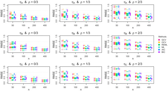
Figure 2.
Simulation RMSE results. Boxplots of the RMSE across the 1000 simulation replications for homoscedastic Gaussian errors. The rows show the results for the mean functions, and the columns show the results for the autocorrelation parameters.
Figure 3 displays the coverage of the 95% Bayesian confidence intervals for each tuning method in each combination of data generating function , autocorrelation , and sample size n when the errors are Gaussian and homoscedastic. The results reveal that the performance of the Bayesian confidence intervals depends on the combination of the function smoothness, the error autocorrelation, the sample size, and the chosen tuning method. When there is no autocorrelation present, all of the tuning methods except the BIC tend to produce better coverage rates (i.e., closer to the nominal level) as the sample size n increases, regardless of the function smoothness. Furthermore, when there is no autocorrelation present, the maximum likelihood methods and the BIC result in noteworthy under-coverage when the function is jagged and the sample size is small. When there exists moderate autocorrelation in the errors (i.e., ), all of the tuning methods result in noteworthy under-coverage, with the maximum likelihood methods performing better for smooth functions and the cross-validation methods performing better for more jagged functions. When the autocorrelation is larger (i.e., ), all of the methods have similarly poor performance.
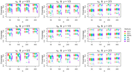
Figure 3.
Simulation coverage results. Boxplots of the coverage rate for the 95% Bayesian confidence intervals across the 1000 simulation replications for homoscedastic Gaussian errors. The rows show the results for the mean functions, and the columns show the results for the autocorrelation parameters.
Our discussion of the results focused on a subset of the simulation conditions, which are sufficient for understanding the primary findings of the simulation study. Specifically, we focused on the results when the errors are Gaussian with constant variance, whereas the results for non-Gaussian and heteroscedastic errors are presented in Appendix A (Gaussian), Appendix B (), and Appendix C (uniform). Interestingly, we found that the RMSE and coverage results were quite similar for the non-Gaussian and heteroscedastic cases. In other words, the primary conclusions that were made about the results in Figure 2 and Figure 3 also apply to the results for non-Gaussian distributions with non-constant variance. When the errors followed a multivariate distribution, the RMSE values tended to be a bit larger for all methods, which is not surprising. However, the primary conclusions regarding the effect of autocorrelation remained the same. It is rather interesting to note that the REML criterion tends to perform relatively well—especially in the presence of autocorrelation in the errors—even when the errors do not follow a Gaussian distribution. Consequently, the REML criterion seems to be a reasonable default tuning criterion as long as the sample size is not too small.
5. Real Data Examples
5.1. Global Warming Example
Our first example uses global land–ocean temperature data, which are freely available from NASA’s Goddard Institute for Space Studies [49,50]. The dataset contains the global land–ocean temperature index from the years 1880 to 2020. Note that the global land–ocean temperature index is the change in global surface temperatures (in degree Celsius) relative to the 1951–1980 average temperatures. Positive values indicate that the average temperature for a given year was above the average temperature for the years 1951–1980, and negative values indicate that the average temperature for a given year was below the average temperature for the years 1951–1980. In our example, we compare the results of the trend estimate using the GCV and REML criteria for selecting the tuning parameter of the smoothing spline. We use the .nknots.smspl function in R [20] to select the number of knots, which results in the selection of 76 knots. For both tuning methods, we use the same 76 knot values to fit the cubic smoothing spline.
The results are plotted in Figure 4, which reveals that the GCV and REML tuning methods produce drastically different pictures of the temperature change across time. Although both methods show that the global land–ocean temperature index has increased over time (particularly since the 1970s), the GCV and REML solutions tell notably different stories about the nature of the increase. The GCV solution has an estimated degrees of freedom of and suggests that the temperature index is rather volatile from year to year. In contrast, the REML solution has an estimated degrees of freedom of and suggests that the temperature index changes in a rather smooth fashion from year to year. Based on the simulation results, it seems likely that the GCV criterion is under-smoothing the data, which may have some noteworthy autocorrelation in the error structure. Consequently, we contend that the REML solution should be preferred for interpreting the nature of the yearly changes in the global land–ocean temperature index.

Figure 4.
Global warming results. Smoothing spline solution for temperature data using GCV tuning (left) and REML tuning (right). Created using the ss() function in the npreg R package [48].
5.2. Motorcycle Accident Example
Our second example uses acceleration data from a simulated motorcycle accident. This dataset was first considered by Silverman [51] and has since been popularized via its inclusion in the popular MASS R package (see mcycle, [52]). The dataset contains the head acceleration (in g) as a function of time (in milliseconds) for points of simulated data. The data are meant to simulate the acceleration curve of the head after a motorcycle accident and were simulated for the purpose of evaluating motorcycle helmets. Due to the simulation procedure, the resulting data are noisy realizations of the true acceleration curve, so the data need to be smoothed in order to estimate the expected head acceleration as a function of time. As in the previous example, (i) we compare the results of the curve estimate using the GCV and REML criteria for selecting the tuning parameter of the smoothing spline and (ii) we use the .nknots.smspl function in R to select the number of knots, which resulted in the selection of 61 knots. For both tuning methods, we use the same 61 knot values to fit the cubic smoothing spline.
The results are plotted in Figure 5, which reveals that the GCV and REML tuning methods produce rather similar estimates in this case. The GCV criterion selected a slightly smaller degree of freedom estimate compared with the REML solution . However, from a practical perspective, the two tuning methods result in smoothing spline estimates that produce the same interpretation of the acceleration curve. The estimated acceleration curve reveals that the head experiences negative acceleration (15–30 ms) followed by a rebound effect of positive acceleration (30–40 ms) before loosely stabilizing around zero ( ms). Finally, it is worth noting that the data in this example violate the homogeneity of variance assumption, which is required for the Bayesian confidence intervals. Therefore, although the GCV and REML tuning criteria may provide satisfactory estimates of the acceleration curve, the Bayesian confidence intervals do not provide satisfactory estimates of uncertainty—in this case, they suggest too much uncertainty in the estimate from 0 to 15 ms.

Figure 5.
Motorcycle accident results. Smoothing spline solution for motorcycle data using GCV tuning (left) and REML tuning (right). Created using the ss() function in the npreg R package [48].
6. Discussion
6.1. Overview
Due to their unique combination of flexibility and interpretability, smoothing splines are frequently used to understand functional relationships in applied research. Unlike standard parametric regression methods (which make strict assumptions) and standard machine learning methods (which produce black-box predictions), smoothing splines are able (i) to learn functional forms and (ii) to produce insightful visualizations. To provide a valid estimate of unknown functional relationships, the smoothing spline estimator requires selecting a smoothing parameter that provides the “correct” balance between fitting and smoothing the data. Specifically, the success of a smoothing spline depends on choosing the tuning parameter that satisfies a Goldilocks phenomenon: if is too small, the estimator has too much variance, and if is too large, the estimator has too much bias. Despite the well-known importance of selecting the “correct” , there is little agreement in the literature regarding which method should be used. Tuning methods can produce different results [26,27] so the choice of tuning method matters.
To address this issue, we explored the relative performance of six popular methods used to select the smoothing parameter . Unlike previous studies on this topic, (i) we compared a diverse collection of tuning methods, which included cross-validation, information theoretic, and maximum likelihood methods; (ii) we designed an extensive simulation study that evaluated each method’s performance under a variety of data generating conditions; and (iii) we assessed the performance of the methods with respect to both function estimation and statistical inference. Furthermore, we used both simulated and real data examples to demonstrate the substantial differences that different smoothing methods can have on the solution. As we elaborate in the following paragraphs, the primary take-home message from our work is that any real data application should compare the results using both the GCV and REML smoothing parameter selection criteria—which is rarely performed in practice.
6.2. Summary of Results
Our simulation results replicate several important findings and provide novel insights about the performance of different tuning methods for smoothing splines. The finding that common tuning methods (i.e., OCV, GCV, and AIC) can breakdown in the presence of autocorrelated errors replicates several past studies on the topic [21,22]. Furthermore, our finding that the REML and ML tuning criteria are relatively robust in the presence of autocorrelated errors supports the theoretical results of Krivobokova and Kauermann [27]. In addition to replicating these known results, our simulation produced several important and novel findings: (i) the performance of the Bayesian confidence intervals deteriorates as the degree of autocorrelation increases; (ii) the cross-validation tuning methods only show an advantage over REML/ML when n is small, is rough, and ; and (iii) the superior performance of the REML/ML tuning methods persists even when the errors are non-Gaussian and/or heteroscedastic.
Our real data results demonstrate the important role that the smoothing parameter selection method plays in understanding functional relationships from a fit smoothing spline. Using the GCV versus the REML criterion, a researcher would arrive at a remarkably different interpretation of the global warming trends. Since these are real data, we cannot be sure whether the GCV or REML solution is closer to the truth. However, in this case, it seems likely that the GCV criterion has capitalized on autocorrelation in the error terms, which manifests itself as a part of the mean structure. In contrast, the REML solution seems to provide a rather parsimonious and intuitive estimate of the global warming trends, which agrees with visual intuition about the nature of the trends across time. Of course, the specifics of the global warming example do not generalize to other datasets, e.g., the two tuning methods performed similarly for the motorcycle data. However, this example illustrates how (i) the GCV criterion can under-smooth data and (ii) the REML criterion can overcome this under-smoothing issue.
6.3. Limitations and Future Directions
This paper only considers the nonparametric regression model in Equation (2), where the unknown function describes the conditional mean of Y given X. Accordingly, this paper only compares tuning methods that are applicable to the penalized least squares problem in Equation (3). Although quite general, the model in Equation (2) can be extended in a variety of different ways. For example, in a generalized nonparametric regression model, the function describes the conditional mean of an exponential family response variable as a function of a predictor [16]. As another example, in nonparametric quantile regression, the function describes the conditional quantile of a response variable as a function of a predictor [53]. Furthermore, penalized splines can be incorporated into other types of nonparametric estimators, e.g., M-estimators [54]. These extensions require different estimation and tuning methods, so the results in this paper cannot be generalized to such extensions. Thus, future work is needed to determine which tuning methods should be preferred when penalized splines are used for various FDA extensions of the simple nonparametric regression model in Equation (2).
6.4. Conclusions
When using smoothing splines for real data analysis, it seems that many researchers do not give much thought to the smoothing parameter selection method. This is likely because many software implementations of smoothing splines do not emphasize the importance of the tuning method. Furthermore, most softwares only implement one or two tuning methods, so researchers rarely have the option to explore a multitude of tuning methods. For example, the smooth.spline() function in R [20] only offers the OCV and GCV tuning methods, and most users seem to (purposefully or unwittingly) use the default GCV tuning method. It is important to note that the GCV method is also the default in the mgcv R package [55], the bigsplines R package [56], and the npreg R package [48]; however, these packages offer more tuning options. For a flexible alternative to R’s smooth.spline() function, we recommend the ss() function from the npreg package, given that it has nearly identical syntax to the smooth.spline() function and makes it possible to easily compare the results using multiple tuning criteria.
Author Contributions
Conceptualization, L.N.B. and N.E.H.; methodology, L.N.B. and N.E.H.; software, N.E.H.; validation, L.N.B. and N.E.H.; formal analysis, L.N.B. and N.E.H.; investigation, L.N.B. and N.E.H.; resources, L.N.B. and N.E.H.; data curation, L.N.B. and N.E.H.; writing—original draft preparation, L.N.B.; writing—review and editing, L.N.B. and N.E.H.; visualization, L.N.B. and N.E.H.; supervision, N.E.H.; project administration, N.E.H.; funding acquisition, N.E.H. All authors have read and agreed to the published version of the manuscript.
Funding
This research was funded by the following National Institutes of Health (NIH) grants: R01EY030890, R01MH115046, U01DA046413, and R01MH112583.
Data Availability Statement
The supporting materials published with this paper include the data and R code needed to reproduce the simulation and real data results. The global temperature anomaly data were obtained from https://data.giss.nasa.gov/gistemp/ accessed on 17 May 2021.
Conflicts of Interest
The authors declare no conflict of interest.
Abbreviations
The following abbreviations are used in this manuscript:
| OCV | Ordinary Cross-Validation |
| GCV | Generalized Cross-Validation |
| AIC | An Information Criterion |
| BIC | Bayesian Information Criterion |
| ML | Maximum Likelihood |
| REML | Restricted Maximum Likelihood |
| RMSE | Root Mean Squared Error |
Appendix A. Supplementary Results for Gaussian Errors
Appendix A.1. RMSE Results
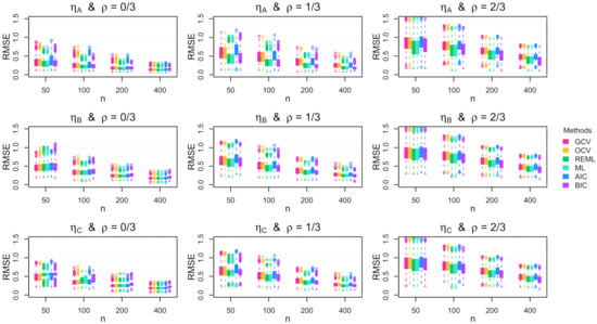
Figure A1.
Boxplots of the root mean squared error (RMSE) across the 1000 simulation replications for Gaussian errors with increasing standard deviation.
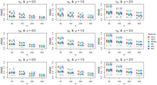
Figure A2.
Boxplots of the root mean squared error (RMSE) across the 1000 simulation replications for Gaussian errors with parabolic standard deviation.
Appendix A.2. Coverage Results
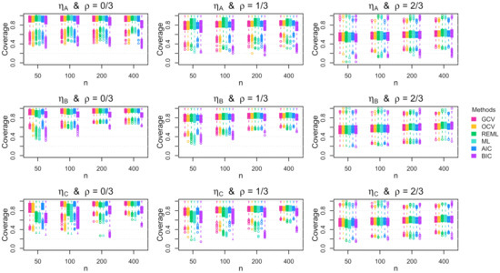
Figure A3.
Boxplots of the coverage rate for the 95% Bayesian confidence interval across the 1000 simulation replications for Gaussian errors with increasing standard deviation.
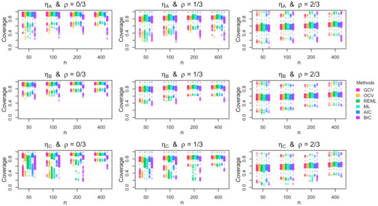
Figure A4.
Boxplots of the coverage rate for the 95% Bayesian confidence interval across the 1000 simulation replications for Gaussian errors with parabolic standard deviation.
Appendix B. Supplementary Results for Multivariate t5 Errors
Appendix B.1. RMSE Results
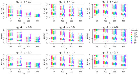
Figure A5.
Boxplots of the root mean squared error (RMSE) across the 1000 simulation replications for multivariate errors with constant standard deviation.
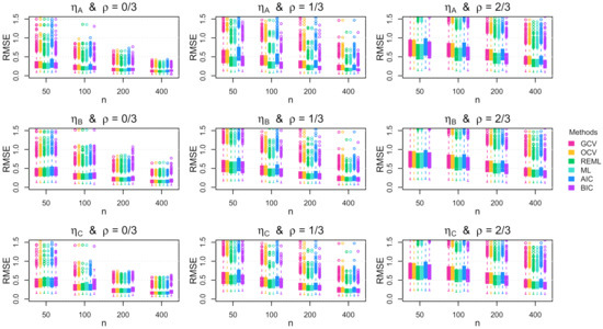
Figure A6.
Boxplots of the root mean squared error (RMSE) across the 1000 simulation replications for multivariate errors with increasing standard deviation.
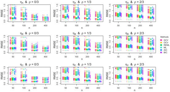
Figure A7.
Boxplots of the root mean squared error (RMSE) across the 1000 simulation replications for multivariate errors with parabolic standard deviation.
Appendix B.2. Coverage Results
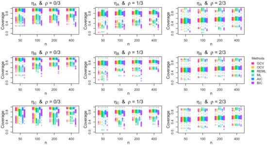
Figure A8.
Boxplots of the coverage rate for the 95% Bayesian confidence interval across the 1000 simulation replications for multivariate errors with constant standard deviation.
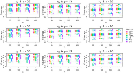
Figure A9.
Boxplots of the coverage rate for the 95% Bayesian confidence interval across the 1000 simulation replications for multivariate errors with increasing standard deviation.
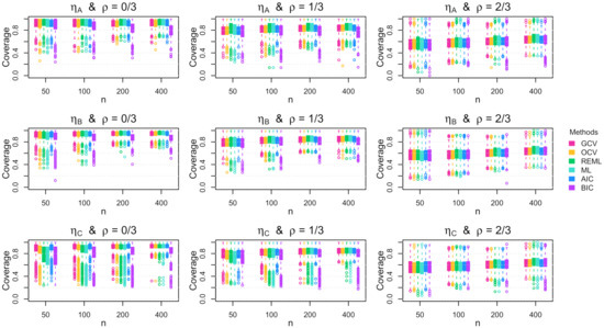
Figure A10.
Boxplots of the coverage rate for the 95% Bayesian confidence interval across the 1000 simulation replications for multivariate errors with parabolic standard deviation.
Appendix C. Supplementary Results for Uniform Errors
Appendix C.1. RMSE Results
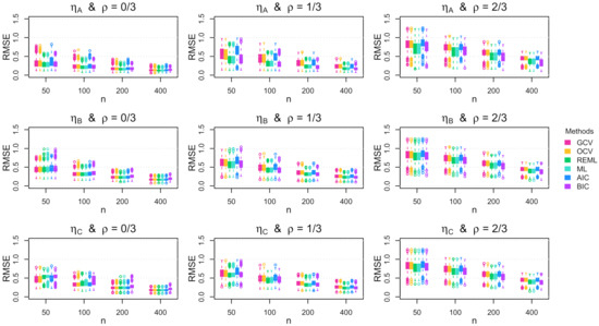
Figure A11.
Boxplots of the root mean squared error (RMSE) across the 1000 simulation replications for uniform errors with constant standard deviation.
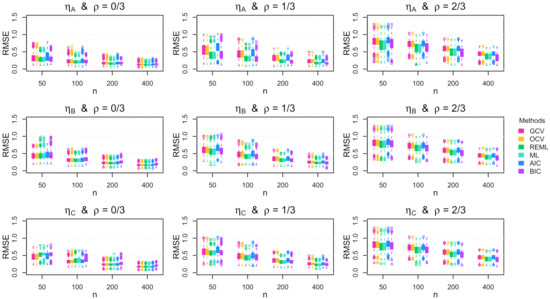
Figure A12.
Boxplots of the root mean squared error (RMSE) across the 1000 simulation replications for uniform errors with increasing standard deviation.
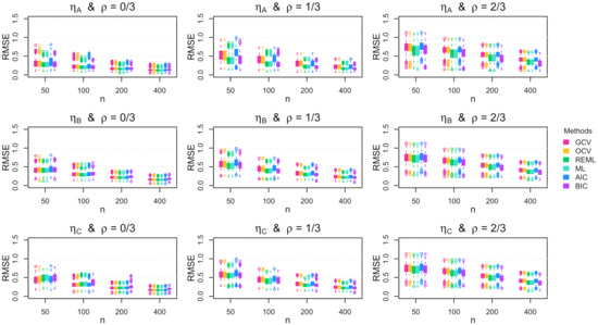
Figure A13.
Boxplots of the root mean squared error (RMSE) across the 1000 simulation replications for uniform errors with parabolic standard deviation.
Appendix C.2. Coverage Results
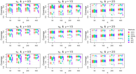
Figure A14.
Boxplots of the coverage rate for the 95% Bayesian confidence interval across the 1000 simulation replications for uniform errors with constant standard deviation.
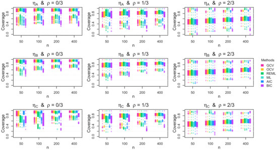
Figure A15.
Boxplots of the coverage rate for the 95% Bayesian confidence interval across the 1000 simulation replications for uniform errors with increasing standard deviation.
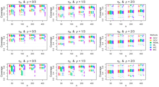
Figure A16.
Boxplots of the coverage rate for the 95% Bayesian confidence interval across the 1000 simulation replications for uniform errors with parabolic standard deviation.
References
- Ramsay, J.O.; Silverman, B.W. Applied Functional Data Analysis; Springer: New York, NY, USA, 2002. [Google Scholar]
- Ramsay, J.O.; Silverman, B.W. Functional Data Analysis, 2nd ed.; Springer: New York, NY, USA, 2005. [Google Scholar]
- Ramsay, J.O.; Hooker, G.; Graves, S. Functional Data Analysis with R and MATLAB; Springer: New York, NY, USA, 2009. [Google Scholar]
- Ullah, S.; Finch, C.F. Applications of functional data analysis: A systematic review. BMC Med. Res. Methodol. 2013, 13, 43. [Google Scholar] [CrossRef] [Green Version]
- Wang, J.L.; Chiou, J.M.; Müller, H.G. Functional Data Analysis. Annu. Rev. Stat. Its Appl. 2016, 3, 257–295. [Google Scholar] [CrossRef] [Green Version]
- Stone, A.A.; Shiffman, S. Ecological momentary assessment (EMA) in behavorial medicine. Ann. Behav. Med. 1994, 16, 199–202. [Google Scholar] [CrossRef]
- Shiffman, S.; Stone, A.A.; Hufford, M.R. Ecological Momentary Assessment. Annu. Rev. Clin. Psychol. 2008, 4, 1–32. [Google Scholar] [CrossRef]
- Helwig, N.E.; Gao, Y.; Wang, S.; Ma, P. Analyzing spatiotemporal trends in social media data via smoothing spline analysis of variance. Spat. Stat. 2015, 14, 491–504. [Google Scholar] [CrossRef]
- Helwig, N.E.; Shorter, K.A.; Hsiao-Wecksler, E.T.; Ma, P. Smoothing spline analysis of variance models: A new tool for the analysis of cyclic biomechaniacal data. J. Biomech. 2016, 49, 3216–3222. [Google Scholar] [CrossRef] [Green Version]
- Helwig, N.E.; Sohre, N.E.; Ruprecht, M.R.; Guy, S.J.; Lyford-Pike, S. Dynamic properties of successful smiles. PLoS ONE 2017, 12, e0179708. [Google Scholar] [CrossRef] [PubMed] [Green Version]
- Helwig, N.E.; Ruprecht, M.R. Age, gender, and self-esteem: A sociocultural look through a nonparametric lens. Arch. Sci. Psychol. 2017, 5, 19–31. [Google Scholar] [CrossRef]
- Lawrence, R.L.; Sessions, W.C.; Jensen, M.C.; Staker, J.L.; Eid, A.; Breighner, R.; Helwig, N.E.; Braman, J.P.; Ludewig, P.M. The effect of glenohumeral plane of elevation on supraspinatus subacromial proximity. J. Biomech. 2018, 79, 147–154. [Google Scholar] [CrossRef] [PubMed]
- Almquist, Z.W.; Helwig, N.E.; You, Y. Connecting Continuum of Care point-in-time homeless counts to United States Census areal units. Math. Popul. Stud. 2020, 27, 46–58. [Google Scholar] [CrossRef]
- Hammell, A.E.; Helwig, N.E.; Kaczkurkin, A.N.; Sponheim, S.R.; Lissek, S. The temporal course of over-generalized conditioned threat expectancies in posttraumatic stress disorder. Behav. Res. Ther. 2020, 124, 103513. [Google Scholar] [CrossRef] [PubMed]
- Helwig, N.E. Regression with ordered predictors via ordinal smoothing splines. Front. Appl. Math. Stat. 2017, 3, 15. [Google Scholar] [CrossRef] [Green Version]
- Helwig, N.E. Multiple and Generalized Nonparametric Regression. In SAGE Research Methods Foundations; Atkinson, P., Delamont, S., Cernat, A., Sakshaug, J.W., Williams, R.A., Eds.; SAGE: Thousand Oaks, CA, USA, 2020. [Google Scholar] [CrossRef]
- James, G.; Witten, D.; Hastie, T.; Tibshirani, R. An Introduction to Statistical Learning, with Applications in R; Springer: New York, NY, USA, 2013. [Google Scholar] [CrossRef]
- Hoerl, A.; Kennard, R. Ridge regression: Biased estimation for nonorthogonal problems. Technometrics 1970, 12, 55–67. [Google Scholar] [CrossRef]
- Gu, C.; Kim, Y.J. Penalized likelihood regression: General formulation and efficient approximation. Can. J. Stat. 2002, 30, 619–628. [Google Scholar] [CrossRef] [Green Version]
- R Core Team. R: A Language and Environment for Statistical Computing; R Foundation for Statistical Computing; R Version 4.1.0; R Core Team: Vienna, Austria, 2021. [Google Scholar]
- Altman, N.S. Kernel smoothing of data with correlated errors. J. Am. Stat. Assoc. 1990, 85, 749–759. [Google Scholar] [CrossRef]
- Opsomer, J.; Wang, Y.; Yang, Y. Nonparametric regression with correlated errors. Stat. Sci. 2001, 16, 134–153. [Google Scholar] [CrossRef]
- Wang, Y. Mixed effects smoothing spline analysis of variance. J. R. Stat. Soc. Ser. B 1998, 60, 159–174. [Google Scholar] [CrossRef]
- Wang, Y. Smoothing spline models with correlated random errors. J. Am. Stat. Assoc. 1998, 93, 341–348. [Google Scholar] [CrossRef]
- Zhang, D.; Lin, X.; Raz, J.; Sowers, M. Semiparametric stochastic mixed models for longitudinal data. J. Am. Stat. Assoc. 1998, 93, 710–719. [Google Scholar] [CrossRef]
- Reiss, P.T.; Ogden, R.T. Smoothing parameter selection for a class of semiparametric linear models. J. R. Stat. Soc. Ser. B 2009, 71, 505–523. [Google Scholar] [CrossRef]
- Krivobokova, T.; Kauermann, G. A note on penalized spline smoothing with correlated errors. J. Am. Stat. Assoc. 2007, 102, 1328–1337. [Google Scholar] [CrossRef]
- Lee, T.C.M. Smoothing parameter selection for smoothing splines: A simulation study. Comput. Stat. Data Anal. 2003, 42, 139–148. [Google Scholar] [CrossRef]
- Kimeldorf, G.; Wahba, G. Some results on Tchebycheffian spline functions. J. Math. Anal. Appl. 1971, 33, 82–95. [Google Scholar] [CrossRef] [Green Version]
- Kim, Y.J.; Gu, C. Smoothing spline Gaussian regression: More scalable computation via efficient approximation. J. R. Stat. Soc. Ser. B 2004, 66, 337–356. [Google Scholar] [CrossRef] [Green Version]
- Gu, C. Smoothing Spline ANOVA Models, 2nd ed.; Springer: New York, NY, USA, 2013. [Google Scholar] [CrossRef]
- Moore, E.H. On the reciprocal of the general algebraic matrix. Bull. Am. Math. Soc. 1920, 26, 394–395. [Google Scholar] [CrossRef]
- Penrose, R. A generalized inverse for matrices. Math. Proc. Camb. Philos. Soc. 1955, 51, 406–413. [Google Scholar] [CrossRef] [Green Version]
- Wahba, G. Bayesian “confidence intervals” for the cross-validated smoothing spline. J. R. Stat. Soc. Ser. B 1983, 45, 133–150. [Google Scholar] [CrossRef]
- Nychka, D. Bayesian confidence intervals for smoothing splines. J. Am. Stat. Assoc. 1988, 83, 1134–1143. [Google Scholar] [CrossRef]
- Kalpić, D.; Hlupić, N. Multivariate Normal Distributions. In International Encyclopedia of Statistical Science; Lovric, M., Ed.; Springer: Berlin/Heidelberg, Germany, 2011; pp. 907–910. [Google Scholar] [CrossRef]
- Allen, D.M. The relationship between variable selection and data augmentation and a method for prediction. Technometrics 1974, 16, 125–127. [Google Scholar] [CrossRef]
- Stone, M. Cross-validatory choice and assessment of statistical predictions. J. R. Stat. Soc. Ser. B (Methodol.) 1974, 36, 111–133. [Google Scholar] [CrossRef]
- Wahba, G.; Wold, S. A completely automatic French curve: Fitting spline functions by cross validation. Commun. Stat. 1975, 4, 1–17. [Google Scholar] [CrossRef]
- Craven, P.; Wahba, G. Smoothing noisy data with spline functions: Estimating the correct degree of smoothing by the method of generalized cross-validation. Numer. Math. 1979, 31, 377–403. [Google Scholar] [CrossRef]
- Li, K.C. Asymptotic optimality for Cp, CL, cross-validation and generalized cross-validation: Discrete index set. Ann. Stat. 1987, 15, 958–975. [Google Scholar] [CrossRef]
- Akaike, H. A new look at the statistical model identification. IEEE Trans. Autom. Control 1974, 19, 716–723. [Google Scholar] [CrossRef]
- Schwarz, G.E. Estimating the dimension of a model. Ann. Stat. 1978, 6, 461–464. [Google Scholar] [CrossRef]
- Wahba, G. A comparison of GCV and GML for choosing the smoothing parameters in the generalized spline smoothing problem. Ann. Stat. 1985, 4, 1378–1402. [Google Scholar] [CrossRef]
- Ruppert, D.; Wand, M.P.; Carroll, R.J. Semiparametric Regression; Cambridge University Press: Cambridge, UK, 2003. [Google Scholar]
- Patterson, H.D.; Thompson, R. Recovery of inter-block information when block sizes are unequal. Biometrika 1971, 58, 545–554. [Google Scholar] [CrossRef]
- Falk, M. A simple approach to the generation of uniformly distributed random variables with prescribed correlations. Commun. Stat.-Simul. Comput. 1999, 28, 785–791. [Google Scholar] [CrossRef]
- Helwig, N.E. npreg: Nonparametric Regression via Smoothing Splines; R Package Version 1.0-6; The Comprehensive R Archive Network. 2021. Available online: https://cran.r-project.org/package=npreg (accessed on 22 August 2021).
- GISTEMP Team. GISS Surface Temperature Analysis (GISTEMP); Dataset Version 4; NASA Goddard Institute for Space Studies. Available online: https://data.giss.nasa.gov/gistemp/ (accessed on 17 May 2021).
- Lenssen, N.; Schmidt, G.; Hansen, J.; Menne, M.; Persin, A.; Ruedy, R.; Zyss, D. Improvements in the GISTEMP uncertainty model. J. Geophys. Res. Atmos. 2019, 124, 6307–6326. [Google Scholar] [CrossRef]
- Silverman, B.W. Aspects of the spline smoothing approach to non-parametric regression curve fitting. J. R. Stat. Soc. Ser. B 1985, 47, 1–52. [Google Scholar] [CrossRef]
- Venables, W.N.; Ripley, B.D. Modern Applied Statistics with S, 4th ed.; Springer: New York, NY, USA, 2002; ISBN 0-387-95457-0. [Google Scholar]
- Koenker, R.; Ng, P.; Portnoy, S. Quantile smoothing splines. Biometrika 1994, 81, 673–680. [Google Scholar] [CrossRef]
- Li, G.Y.; Shi, P.; Li, G. Global convergence rates of B-spline M-estimators in nonparametric regression. Stat. Sin. 1995, 5, 303–318. [Google Scholar]
- Wood, S.N. mgcv: Mixed GAM Computation Vehicle with Automatic Smoothness Estimation; R Package Version 1.8-35; The Comprehensive R Archive Network. 2021. Available online: https://cran.r-project.org/package=mgcv (accessed on 22 August 2021).
- Helwig, N.E. bigsplines: Smoothing Splines for Large Samples; R Package Version 1.1-1; The Comprehensive R Archive Network. 2018. Available online: https://cran.r-project.org/package=bigsplines (accessed on 22 August 2021).
Publisher’s Note: MDPI stays neutral with regard to jurisdictional claims in published maps and institutional affiliations. |
© 2021 by the authors. Licensee MDPI, Basel, Switzerland. This article is an open access article distributed under the terms and conditions of the Creative Commons Attribution (CC BY) license (https://creativecommons.org/licenses/by/4.0/).