Abstract
Expert knowledge elicitation (EKE) aims at obtaining individual representations of experts’ beliefs and render them in the form of probability distributions or functions. In many cases the elicited distributions differ and the challenge in Bayesian inference is then to find ways to reconcile discrepant elicited prior distributions. This paper proposes the parallel analysis of clusters of prior distributions through a hierarchical method for clustering distributions and that can be readily extended to functional data. The proposed method consists of (i) transforming the infinite-dimensional problem into a finite-dimensional one, (ii) using the Hellinger distance to compute the distances between curves and thus (iii) obtaining a hierarchical clustering structure. In a simulation study the proposed method was compared to k-means and agglomerative nesting algorithms and the results showed that the proposed method outperformed those algorithms. Finally, the proposed method is illustrated through an EKE experiment and other functional data sets.
1. Introduction
Even when we receive information under the same conditions, our point of view may greatly differ from others’. Therefore, if we want to analyze expert knowledge, such differences should be considered. Figure 1 shows a representation of this problem. Our point of view on certain information depends on our cognitive skills and external factors that might change our beliefs.
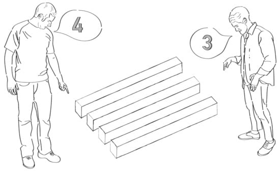
Figure 1.
Illustration of two experts having different points of view in regards to a specific phenomenon.
Expert knowledge elicitation (EKE) has the goal of producing, via elicitation, a probabilistic distribution that represents the expert’s knowledge around a parameter of interest. For that purpose, we can adopt the Delphi method as an elicitation method. The latter is defined by Brown (1968) [1] as a technique based on the results of multiple rounds of questionnaires sent to a panel of experts and whose purpose is to reach a consensus on their opinion. Such method is effective, as it allows a group of individuals to address a complex problem and could be implemented to obtain a single representation of experts’ beliefs through a probability distribution. However, this method proves difficult when the number of experts in the study increases considerably.
Finding the mean of the level of certainty of each expert using their personal distributions is another way to obtain a prior distribution of expert knowledge. Nevertheless, it could be erroneous, as shown in Figure 2, where, for instance, we observe two hypothetical experts’ prior distributions (red and black curves) representing their level of knowledge over a proportion of , and the mean of the level of the two experts (green curve), which does not represent the actual level of certainty of each expert. As a result, the entire complex elicitation work done for each expert is wasted. Hence, we believe that the probability distributions of each expert can be classified and their opinions represented using clusters of beliefs. Thus, Bayesian inference can be carried out in parallel by considering each cluster of priors and a decision can be arrived at via experts’ criteria (Barrera-Causil et al., 2019) [2].
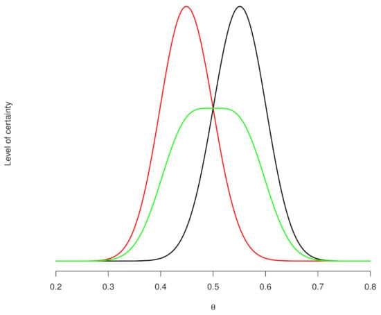
Figure 2.
Level of certainty of two hypothetical experts (red and black curves) and their mean (green curve). Note that, when the location parameters of the experts’ distributions are different, those of the resulting mean distribution (green curve) may be considerably different from the experts’ actual opinion.
On the other hand, classifying probability distributions is an essential task in different areas. Clustering methods to classify word distribution histograms in information retrieval systems have been implemented successfully [3]. For instance, Henderson at al. (2015) [4] present three illustrations with airline route data, IP traffic data, and synthetic data sets to classify distributions. Therefore, functional data analysis (FDA) could be used for clustering distributions since it is an extension of the multivariate methods where observations are represented by curves in a function space [5]. Some tools of multivariate analysis have been extended to the functional context pointwise, considering the implementation of multivariate procedures around the real interval where these functions are defined. Thus, in many cases, the curves are discretized to implement statistical procedures.
Cluster analysis is one of multiple techniques that have been extended to FDA, and different methods are implemented to obtain partitions of curves within its framework. Some of those methods have been compared to determine their performance and make recommendations in several situations [6]. For instance, Abraham et al. [7] proposed a two-stage clustering procedure in which each observation is approximated by a B-spline in the first stage, and the functions are grouped using the k-means algorithm in the second stage. Gareth and Sugar (2003) [8] presented a model-based approach for clustering functional data. Their method was effective when the observations were sparse, irregularly spaced, or occurred at different time points for each subject. Serban and Wasserman (2005) [9] proposed a technique for nonparametrically estimating and clustering a large number of curves. In their method, the nearly flat curves are removed from the analysis, while the remaining curves are smoothed and finally grouped into clusters.
Other alternatives can also be found in the literature. For instance, Shubhankar and Bani (2006) [10] proposed a nonparametric Bayes wavelet model for clustering curves based on a mixture of Dirichlet processes. Song et al., (2007) [11] presented a FDA-based method to cluster time-dependent gene expression profiles. Chiou et al. (2007) [12] developed a Functional Clustering (FC) method (i.e., k-centres FC) for longitudinal data. Their approach accounts for both the means and the modes of variation differentials between clusters by predicting cluster membership with a reclassification step. Tarpey (2007) [13] applied the k-means algorithm for clustering curves under linear transformations of their regression coefficients. More recently, Goia et al., (2010) [14] used a functional clustering procedure to classify curves representing the maximum daily demand for heating measurements in a district heating system. Hébrail et al., (2010) [15] proposed an exploratory analysis algorithm for functional data. Their method involves finding k clusters in a set of functions and representing each cluster with a piecewise constant, seeking simplicity in the construction of the clusters. Boullé (2012) [16] presented a novel method to analyze and summarize a collection of curves based on a piecewise constant density estimation where the curves are partitioned into clusters. Furthermore, Secchi et al., (2012) [17] focused on the problem of clustering functional data indexed by the sites of a spatial finite lattice. Jacques and Preda (2013) [18] presented a model-based clustering algorithm for multivariate functional data based on multivariate functional principal components analysis. The references in Jacques and Preda (2013) [19] are of particular importance because they summarize the main contributions in the field of functional data clustering. Other clustering algorithms have been reported in the literature. For instance, Ferreira and Hitchcock (2009) [6] compared four hierarchical clustering algorithms on functional data: single linkage, complete linkage, average linkage, and Ward’s method (T these methods are implemented in the agnes function of R. This function takes several arguments: x, a data matrix, data frame, or dissimilarity matrix; metric which is the metric to be used for calculating dissimilarities between observations (by default, it is the euclidean distance); and method, a character string specifying the clustering method (single linkage, complete linkage, average linkage, or Ward’s method)). Ferreira and Hitchcock (2009) [6] found that Ward’s method and average linkage outperform their counterparts.
Although there is research relating to the clustering of functions, no study has considered functional clustering of experts’ beliefs. For example, Stefan et al., (2021) [20] studied the effect of interpersonal variation in elicited prior distributions on Bayesian inference. In their study one of the six experts exhibited discrepant distributions. Thus, it would be ideal to have a method able to numerically address discrepancies among clusters of elicited prior distributions. Another important situation is when a researcher needs to make a decision based on information obtained from elicited priors. In all these cases, and according to the problem showed in Figure 2, differences between priors should be addressed and the estimation, either posterior or prior, must be done in parallel for each group of elicited priors. Thus, in this paper we propose a new method to deal with multiple elicited prior distributions. The method thus allows clustering distributions using FDA and the Hellinger’s distance (Simpson, 1987) [21]. Hellinger’s distance enables to quantify the similarity between two probability distributions and, we believe, it is a more appropriate metric than the current metrics for functional data. An illustration of the place of the proposed method within the expert knowledge elicitation workflow is shown in Figure 3.
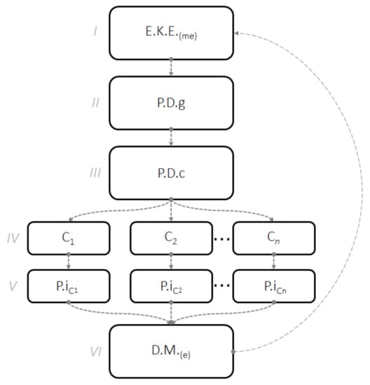
Figure 3.
Illustration of the expert knowledge elicitation workflow. = expert knowledge elicitation from multiple experts; = generation of prior distributions; = clustering of prior distributions; = cluster 1 to cluster n; = prior or posterior inference for each cluster; = decision making with a panel of experts. The long dash arrow from to indicates that workflow can be iterated if required. The goal of the workflow is to create clusters of experts and analyze the clusters separately by means of prior or posterior estimations. A final decision is reached via a panel of experts. Step IV is unique to our proposal in that it shows where the clustering of elicited prior distributions takes place in the EKE workflow.
This proposal is motivated by the interest of offering a new tool for the analysis of prior curves from multiple experts when elicitation is used. However, in addition to offering an alternative to the problem posed in Figure 2, or to the complexity involved in applying the Delphi method with a considerable number of experts, this proposal can be implemented to detect atypical curves, or even to create clusters in fuzzy multicriteria decision-making problems (Kahraman, Onar, and Oztaysi, 2015) [22].
To test the efficiency of the clustering algorithm our method, we propose a hierarchical clustering technique for functional data and compare it, via statistical simulation, with functional k-means, Ward’s, and average linkage methods (these methods are implemented in R [23] through thekmeans.fd function in the fda.usc package (Febrero-Bande and Oviedo, 2012) [24] and the agnes function in the cluster package [25]. The latter function performs agglomerative nesting clustering). To examine the similarity between two clusters, we considered the Rand index, the Fowlkes–Mallows index, the Jaccard coefficient—index to measure similarity between sample sets—and the correct classification rate (Hubert and Arabie, 1985; Morlini and Zani, 2012) [26,27]. Note that reporting the outcomes of all these indexes allows seeing patterns in the results and it is in line with practices to enhance transparency in research (Steegen et al., 2016) [28]. Finally, the application of our method is illustrated using real data sets.
The paper is structured as follows: Section 2 introduces some theoretical approaches and details the proposed method for clustering density functions and/or functional data. Section 3 describes the simulation study and its results. Section 4 shows an example using real data sets to illustrate the use of the proposed method. Section 5 presents the main contributions of this paper and suggests topics for further research. Finally, Section 6 contains the supplementary material and three additional illustrations using different data sets (see Appendix A).
2. Definitions
2.1. Elicitation of Probability Distributions
An elicitation process involves extracting information about parameters of interest () from the subjective experience of a person (expert) and expressing it as a probability distribution (prior distribution) Barrera-Causil et al., (2019) [2]. Thus, for expert i, a real function (prior distribution) is elicited, and for a grid of m equally spaced points () throughout the support of this distribution, the heights of the function are calculated . This process is made for n experts with the aim to discretize the functions .
2.2. Functional Data Analysis
In functional data, the ith observation is a real function , where , such that and are the minimum and maximum of for the i-th expert, respectively, and is a real interval . Thus, each is a point in certain function space (Ramsay et al. 2009) [29]. For analysis purposes, we assume that the functional data has an inner product or Hilbert space structure, that is, , where is a vector space of functions defined on a real interval and is complete and has an inner product .
Functional Clustering
There are different methods for clustering functional data, such as k-means, agnes with the agglomerative average method, and Ward’s method, among others (Ferreira and Hitchcock (2009) [6]). However, k-means is used most frequently.
Table 1 describes three different methods implemented in this paper.

Table 1.
Methods for clustering functional data.
2.3. Proposed Method
Our proposed method for clustering density functions, based on the Hellinger distance, works as follows:
- 1.
- For each , , discretize the curve and get a grid of m equidistant points . These points correspond to heights of the curve in m equally spaced points of the support of the function (in this paper, we use 200 and 300 equally spaced points throughout the support of the function. The determination of the amount of points depends on computational capacity). Thus, to apply this methodology, we recommend selecting equidistant points throughout the support of the distributions of interest in order to capture the shape of the curves. We have found that increasing the numbers of points does not have a notorious effect on the outcome of the algorithm).
- 2.
- Compute the Hellinger distance for all possible combinations of two of these functions. So, for curves and , the distance is as follows:wherewith and are defined.
- 3.
- Build a matrix of distances between all curves using the proposed metric.
- 4.
- Use the hierarchical clustering function hclust in R with as the distance matrix.
- 5.
- Obtain the corresponding dendrogram.
- 6.
- Specify the number of clusters and identify the members in each cluster.
To analyze the performance of our proposed method, we compared it with other algorithms available in the literature under different schemes. Such algorithms included those implemented in the kmeans.fd and agnes functions in R, as studied by Ferreira and Hitchcock (2009) [6]. In the following section, we explain in detail the way the simulation study was conducted.
3. Simulation Study
For simulation purposes, density functions were used as functional data. The theoretical counterpart of these densities was estimated using kernel functions via the density() function in R. To assess the performance of our method, we compared it with the functional k-means, Ward’s, and average linkage methods for functional data as implemented in the kmeans.fd(), agnes(method="ward") and agnes(method="average") functions in R, respectively. In the simulation study, we generated overlapping distributions and overlapping clusters of distributions based on the two following definitions:
Definition 1.
Overlapping distributions. Let X and Y be random variables with density functions and , respectively, both sharing the same support, and define as the γ-th percentile of Z. Then, we can say that f and g overlap if one of the following conditions is satisfied:
- (a)
- ∧
- (b)
- ∧ .
Definition 2.
Overlapping clusters of distributions. A cluster is δ-overlapped with another one if at least of those distributions is overlapped. If two clusters of distributions are not overlapped, it means they are separated.
Initially, the clusters generated contained a finite number of curves following a Normal distribution with pre-specified means and variances for each real group but with a random perturbation of the parameters within clusters. Therefore, three clusters with curves per cluster were considered. All of the cases above were simulated considering two and three clusters of curves.
We also considered asymmetrical features to compare the behavior of the four methods under different scenarios and thus modified the previously described simulation process (clusters of Normal distributions) using Gamma and Beta distributions within clusters. A further major consideration in all cases was the use of an atypical curve for each simulation scenario to evaluate the performance of the method in the presence of atypical curves. To study the effectiveness of the method under evaluation, we considered separated and -overlapped clusters of distributions with a known value of . The average overlapping rate in each scenario is presented in Table 2.

Table 2.
Average value of in all simulation scenarios.
In all the simulation scenarios, the existence of clusters of curves was ensured by testing the equality of their means. Figure 4 shows one of the different simulation scenarios used to compare the four methods. These scenarios were considered for two and three clusters, with curves per cluster, and an equal number of curves. In each simulation scenario, a total of 1000 replicates were run. To validate the clusters found at each replicate, we used the routines in the clv package [31] in R. The performance of the four methods compared here was assessed using the Rand index, the Fowlkes–Mallows index (F.M), the Jaccard coefficient, and the correct classification rate. These measures are defined by the equations below.
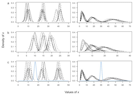
Figure 4.
Illustration of some assessed simulation schemes where three clusters of curves with a (a) separated, (b) overlapped, and (c) atypical structure are generated. Clusters of Normal and Gamma distributions are presented in the first and second columns, respectively. In (c), atypical curves are shown in blue.
Given a set of n elements and two partitions of S to be compared: , a partition of S into r subsets, and , a partition of S into s subsets, define the following:
- a: the number of pairs of elements in S that are in the same set in X and in the same set in Y.
- b: the number of pairs of elements in S where both elements belong to different clusters in both partitions.
- c: the number of pairs of elements in S where both elements belong to the same cluster in partition X but not in partition Y.
- d: the number of pairs of elements in S that are in different sets in X and in the same set in Y.
So,
For some, , , , , , , , , .
The Rand index (R), the Jaccard coefficient (J), the Fowlkes–Mallows index (F.M), and the correct classification rate (CCR) are thus calculated as follows:
All these validation measures have a value between 0 and 1, where 0 indicates that no pair of points is shared by the two data clusters, and 1 means that the data clusters are exactly the same.
Results
The main results of this simulation study are shown in Figure 5 and Figure 6 (R codes and data associated with this article can be found at https://figshare.com/projects/An_FDA-based_approach_for_clustering_expert_knowledge/73437 (accessed on 4 March 2021)). In general, and regardless of the performance index we used, our proposed method performs better than kmean.fd, Ward’s, and average linkage methods in terms of recreating the cluster structure in the data (Figure 5). Therefore, the clustering method based on the Hellinger distance proposed herein is a better choice for classifying density curves (or, for that matter, functional data).
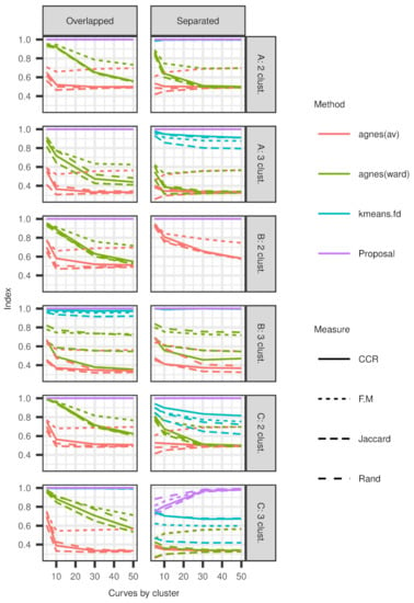
Figure 5.
Performance indexes when two and three clusters of overlapped and separated (A) Normal, (B) Gamma, and (C) Beta distributions are generated.
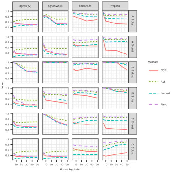
Figure 6.
Performance indexes when two and three clusters of (A) Normal, (B) Gamma, and (C) Beta distributions with one atypical curve are generated.
The assertion above is justified from two perspectives. First, when clusters are separated or overlapped or an atypical curve is present in simulated data from Normal or Gamma populations, there is evidence that our method performs better than the other ones. Second, when two clusters from a Gamma population are generated, the kmean.fd and Ward’s methods, as well as our proposed method, performed equally well. However, in any other scenario, our method outperforms the others.
Although the kmean.fd method and our proposal perform equally well in almost all the scenarios, our method outperforms others when three clusters of Gamma curves are considered regardless of their degree of overlap (Figure 5). When compared with Ward’s method, ours has a slightly lower performance when curves are generated for two clusters of curves obtained from a Gamma distribution. A similar behavior is observed when two clusters of overlapped Beta curves are generated, or when curves from two clusters of a Beta distribution with an atypical curve are generated (Figure 6). In the former case, our proposal exhibits a slightly lower performance than the other alternatives. However, in general, our method and the kmean.fd algorithm performed equally well. In the latter case, Ward’s method performs slightly better than our proposed method.
Figure 6 illustrates the performance measures of the four methods compared in this study to obtain optimal partitions. Overall, all the methods studied here exhibit poor performance compared to that of our proposal. The result seems to be a promissory topic for further exploration, especially for clusters generated from a Beta distribution because this is a very flexible distribution that can take different shapes. The closed support of a Beta distribution leads to seeking clusters under more concentrated possibilities, turning every method into a more overlapping one and making it more challenging to detect the true differences within these curves. Thus, our proposed method exhibits the best performance compared to the other options considered here.
4. Illustration
This section shows the performance of our proposed method when faced with a real data set.
Computer’s Lifetime Elicitation
The purpose of this application is to segment prior distributions of experts regarding a desktop computer’s average operation time in months; since its purchase until its first failure. Those prior distributions were obtained in an elicitation process described in Barrera and Correa (2008) [32]. They carried out this elicitation process through an interview-survey administered to six experts; however, their study was conducted taking into account only the person with the most exceptional expertise. In this study, we work with all prior distributions, considering the possible existence of clusters.
Figure 7 shows the elicited prior distributions (plotted via the free-hand method) of the six experts, which resulted from the interview-survey conducted in Barrera-Causil and Correa (2008) [32]. We can observe that all the distributions have a similar distributional shape, but one of them (in green) has a very different shape with respect to the others. Table 3 shows the experts’ years of experience in the ICT area (expertise) and years in their current job. Expert 3 exhibits the highest level of expertise.
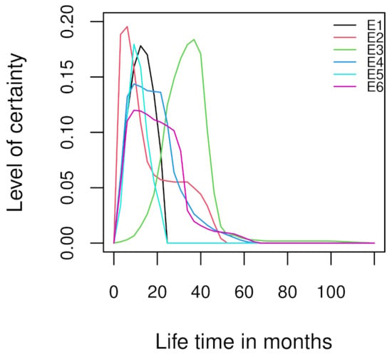
Figure 7.
Prior distributions of the beliefs of six experts.

Table 3.
Experts’ years of experience in the ICT area and years in their current job. Note for example that while E3 and E4 have the same number of years of expertise, E3 has more experience working the computers being assessed in this study.
Applying our proposed clustering method, Figure 8 presents the cluster dendrogram of the six experts, where we can observe that the prior belief of Expert 3 is far from that of the other participants. Furthermore, note that, in Table 3, this expert exhibits the highest level of expertise. For that reason, we decided to analyze the prior distributions using two clusters: one comprising Experts 1, 2, 4, 5 and 6; and another one containing Expert 3 alone.
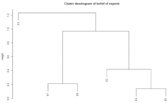
Figure 8.
Cluster dendrogram of the six experts.
In this situation, the following questions arise: Is the average of all distributions the best representation of prior beliefs? Is it possible to reach a consensus among these experts? Regarding the last question, in some cases a consensus can be quickly reached, but in many others this process can be tedious or such agreement cannot be reached.
As for the first question, when priors are very different, the average of these distributions can result in almost an uniform distribution that spoils the complex process of elicitation. Thus, we recommend creating homogeneous groups of these prior distributions and analyzing them simultaneously. To analyze each group simultaneously, we calculate the functional mean and approximate the average curves to a Gamma distribution by cluster. By using the fitdistr function of the R software, we obtain a maximum-likelihood fitting of Gamma distribution for the functional mean in each cluster. This procedure can be described as follows:
- The functional mean is obtained in each cluster.
- 1000 observations are generated from the distribution that is proportional to the the functional mean in each cluster.
- This distribution is approximated to a gamma distribution using the fitdistr function with the generated samples.
Accordingly, for the cluster formed by Experts 1, 2, 4, 5, and 6, the fitted prior distribution is , with standard errors of the estimated parameters 0.39011009 and 0.02798532, respectively. For Expert 3, the fitted distribution is , with standard errors of the estimated parameters 2.04588737 and 0.06345412, respectively (the Gamma distribution was chosen as it is a distribution typically used to model lifetime data (Shanker et al., 2016 [33]). A method based on goodness-of-fit metrics (e.g., AIC) via a GAMLSS approach (see Rigby and Stasinopoulos, 2005) [34] could have suggested distributions other than the Gamma as better fits. Thus, the selection of the distribution has a direct effect on estimates of location, scale, and shape and, in turn, on any subsequent inferential analysis). Figure 9 shows prior distributions, by cluster, of a computer’s average operation time in months (since its acquisition until its first failure) considering the functional mean in each group.
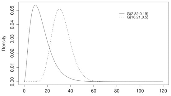
Figure 9.
Prior distributions by cluster of experts. Expert 3 is represented by the dotted PDF and the remaining experts are represented by the solid PDF.
It is clear there are two clusters of experts with their distributions exhibiting differences in location and scale. As mentioned above, combining both distributions is indeed possible (e.g., by averaging); however, doing so does not reflect the level of expertise in each cluster (see Figure 2). Thus, each cluster should be analysed separately. Next, we illustrate a parallel analysis for each cluster. Table 4 shows the lifetime of the desktop computers assessed by the experts in the study by Barrera-Causil and Correa (2008) [32]. By resorting to the exponential component of the Gamma distribution, it is possible to estimate 95% probability intervals for the average time of the first occurrence of a physical failure in a desktop computer (in months). Thus,
where x are the observed data, and is the parameter of interest.

Table 4.
First failure times (in months) of 72 desktops. Out of the 72 desktop computers, 17 desktops were reported to have failed at the time of the study. The failure times of the remaining 55 desktops were denoted by (this indicates that these computers had not failed by the time when the study was carried out).
For cluster 1, as the average operation time in months is , then we have that follows an inverted Gamma distribution. Then, the prior of can be expressed as
Given that the likelihood of the Exponential distribution is
The posterior distribution is therefore:
where .
We know that for future observations y, the predictive distribution is given by
In order to obtain the predictive Bayesian PDF, 1000 samples from the posterior distribution were obtained. Thus, the Bayesian predictive density for cluster 1, can be expressed as:
where .
A 95% probability interval of the average time of the first failure time of a desktop computer (in months) in cluster 1, could be calculated by plugging the 1000 samples from the posterior distribution into the previous equation. The interval in cluster 1 is therefore . By performing the same procedure for cluster 2, the resulting 95% probability interval is . These probability intervals can then be used by a panel of experts to make case-related decisions.
5. Discussion
In this paper, we proposed a simple method to segment expert knowledge that can be effectively applied to functional data or problems with large volumes of data (data mining). Implementing such method, we built, after a discretization process, a distance matrix between curves using the Hellinger distance.
A simulation study considering different scenarios was presented. In such study, our proposed method performed better in almost all scenarios than the k-means and agglomerative nesting clustering algorithms for functional data (as implemented in the kmean.fd and agnes functions in R, respectively). Therefore, it proved to be a useful tool to perform a cluster analysis with distributions elicited from experts’ personal beliefs. Based on the computers’ lifetime example, we conclude that the proposed clustering method can be used to segment expert knowledge. Furthermore, it can identify the expert with the highest level of expertise, which is very important when analyzing experts’ beliefs considering their different points of view.
Along the same lines of this proposal, further research topics in this field include sensitivity analyses when different initial values are considered. Another interesting area, based on the results of the analyses above, is developing a robust clustering method to generate data partitions, namely a clustering method that performs well in different conditions. Additionally, other distributions (e.g., Poisson), samples, and cluster sizes should be considered in future simulation studies to further assess the performance of our method.
Finally, we believe our proposed method has implications for two specific areas; combination of expert knowledge and machine learning (ML), and Bayesian inference. Supervised (e.g., classification) and unsupervised (e.g., clustering) ML methods have gained momentum in current research. For example, it has been shown that ML-based classification ensembles perform better than experts in segregating viable from non-viable embryos [35] and that (evolutionary) clustering algorithms enable characterising COVID-19-related textual tweets in order to assist institutions in making decisions [36]. In general, researchers pitch ML-based analyses against human expert knowledge because they see no value in it or because do not know how to integrate into the analysis pipeline. Evidence, however, suggests that blending expert knowledge with ML analyses leads to better predictions [37,38,39,40]. We believe our proposal can be used to contribute in this rather under-investigated area.
A challenge in Bayesian inference is to determine the effect of different prior distributions on a parameter to be estimated. In this regard, Stefan et al., (2021) [20] found that the variability in prior distributions from six experts did not affect the qualitative conclusions associated to estimated Bayes factors. Their results thus suggest that although there can be quantitative differences between the elicited prior distributions, the overall qualification associated to those quantities is not altered. We believe, though, that if the elicited distributions show considerable fluctuation in terms of location, scale and shape, those distributions need to be subjected to clustering in order to segregate levels of expertise (see Figure 2, Figure 7 and Figure 9). The method proposed herein can serve for such purpose.
6. Conclusions
Although the proposed clustering method is designed for data obtained from experts’ belief curves, we demonstrated it can be applied to data sets that do not correspond to distributions or curves (we show this in three supplementary examples). In conclusion, the proposed method offers encouraging applications using other types of data sets encountered in data mining problems.
Author Contributions
Conceptualisation and methodology, C.B.-C., J.C.C. and F.T.-A.; validation and formal analysis, C.B.-C., F.M.-R.; investigation, C.B.-C.; resources, C.B.-C., F.M.-R.; writing—original draft preparation, C.B.-C., F.M.-R. and A.Z.; writing—review and editing, C.B.-C., F.M.-R. and A.Z.; visualisation, C.B.-C.; supervision, J.C.C.; project administration, C.B.-C.; funding acquisition, C.B.-C. All authors have read and agreed to the published version of the manuscript.
Funding
This research received no external funding.
Institutional Review Board Statement
Not applicable.
Informed Consent Statement
Informed consent was obtained from all subjects involved in the study.
Data Availability Statement
The data presented in this study are openly available in https://figshare.com/projects/An_FDA-based_approach_for_clustering_expert_knowledge/73437 (acessed on 13 December 2020).
Acknowledgments
C.B.-C. thanks Instituto Tecnológico Metropolitano -ITM- for their support. The authors dedicate this work to the memory of prof. Francisco Torres-Avilés. Figure 1 was designed by Daniela Álvarez Lleras (alvarezlleras.daniela@gmail.com) and it is inspired on the impossible trident optical illusion.
Conflicts of Interest
The authors declare that the research was conducted in the absence of any commercial or financial relationships that could be construed as a potential conflict of interest.
Abbreviations
The following abbreviations are used in this manuscript:
| CCR | Correct classification rate |
| FC | Functional clustering |
| FDA | Functional data analysis |
| F.M | Fowlkes–Mallows |
| ICT | Information and communications technology |
| J | Jaccard coefficient |
| R | Rand index |
Appendix A
This section presents the performance of the proposed method in different scientific fields. Note that this proposal was focused on elicited prior distributions, but it could be applied using other types of data sets.
Appendix A.1. Weather Station Density Classification
In this example, we used the CanadianWeather data set from the fda R package. Particularly, we analyzed the average daily temperatures at 35 different locations in Canada from 1960 to 1994. Although this data set has already been studied from different points of view (see Ramsay and Silverman, 2005 [41]; Giraldo, 2009 [42]; and Giraldo, Delicado and Mateu, 2012 [43] for more details), our interest was focused on seeking, for each location, the optimal density clusters associated with the average temperatures in January.
The dendrogram in Figure A1 suggests that the weather stations can be grouped into five clusters. Although this is a subjective criterion, it is an important step to compare the number of clusters defined by our method with the actual grouping of the Canadian geographical locations (see Table A1). An objective alternative to select the numbers of clusters could be applied using a cost function (see Cohen-Addad, 2019 [44]).
Figure A2 shows the density functions of the temperatures at each location (color coded by cluster). Note that, after applying our clustering method, five clusters can be clearly identified in the data even though the spatial correlation effect was not taken into account.
After comparing these results with the actual locations in Figure A3, we found that cluster 1 (C1) represents stations located close to the Atlantic continental coast and surrounding islands (5 cities), two cities near Lake Ontario, and Kamloops—an “atypical” city located in the province of British Columbia. Although Kamloops seems to be an outlier in this group, the behavior of the temperatures in this area is very similar to the one mentioned before (see https://weather.gc.ca/ (acessed on 13 December 2020)).
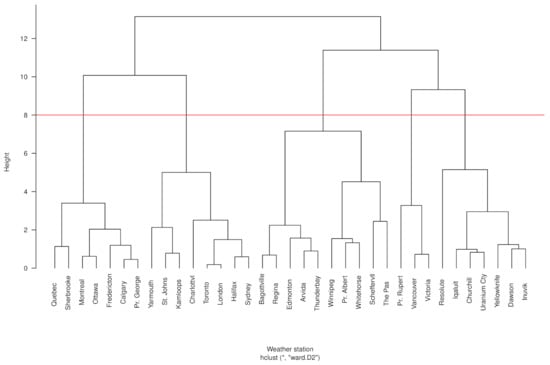
Figure A1.
Dendrogram of Canadian weather stations. The clusters are, from left to right, C2 (from Quebec to Pr. George), C1 (from Yarmouth to Sydney), C3 (from Bagottville to The Pas), C5 (from Pr. Rupert to Victoria), and C4 (from Resolute to Inuvik).
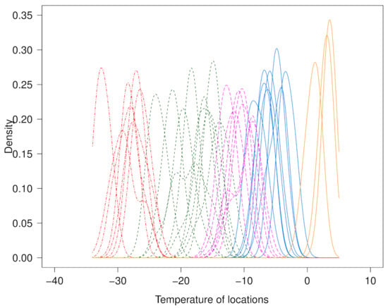
Figure A2.
Densities of the Canadian weather stations by cluster. From left to right, C1: red densities, C2: green densities, C4: purple densities, C3: blue densities, and C5: orange densities.

Table A1.
Clusters resulting from data of Canadian weather stations.
Table A1.
Clusters resulting from data of Canadian weather stations.
| Cluster 1 | Cluster 2 | Cluster 3 | Cluster 4 | Cluster 5 | |
|---|---|---|---|---|---|
| Locations | St. Johns | Fredericton | Scheffervll | Churchill | Vancouver |
| Halifax | Quebec | Arvida | Uranium Cty | Victoria | |
| Sydney | Sherbrooke | Bagottville | Dawson | Pr. Rupert | |
| Yarmouth | Montreal | Thunderbay | Yellowknife | ||
| Charlottvl | Ottawa | Winnipeg | Iqaluit | ||
| Toronto | Calgary | The Pas | Inuvik | ||
| London | Pr. George | Regina | Resolute | ||
| Kamloops | Pr. Albert | ||||
| Edmonton | |||||
| Whitehorse |
Despite certain limitations of the available sample, the classification of these locations based on the proposed method matches, almost entirely, their geographical distribution. For instance, Cluster 2 (C2) is also segmented into two principal areas. The first one includes cities near the river in the East of the country (5 cities) and bordering St. Lawrence River as far as Ottawa; the second one features stations located in cities near the Appalachian Mountains. The stations in Cluster 3 (C3) are located in the Mid-South part of the country. Cities in Cluster 4 (C4) are located in the coldest zones (extended North). Finally, Cluster 5 (C5) consists of cities on the Pacific coast. These results provide us with a good classification/representation of the actual temperature distribution registered at those stations (see Figure A2).
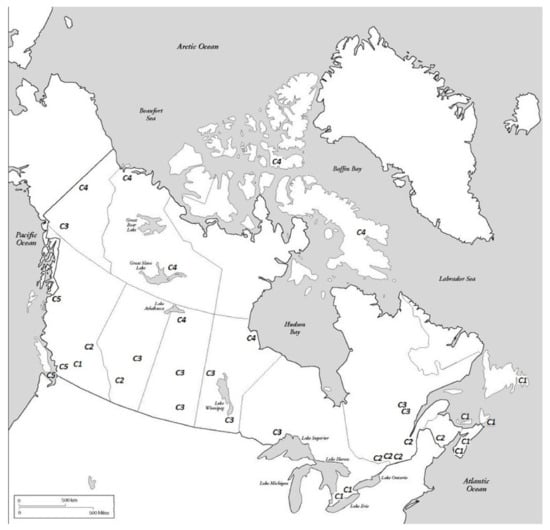
Figure A3.
Map of Canada. The clusters are C1, C2, C3, C4, and C5 (see Table A1 for the list of cities in each cluster and Figure A2 for their temperatures). Adapted from http://goo.gl/Ok8CWv (accessed on 13 December 2021)
Appendix Students Data Set
We collected data of students pursuing an online bachelor’s degree in Health Science at a public university in Australia in 2018. We selected students from an online program instead of an on-campus one due to the increased diversity in demographics (i.e., age groups) Stone (2019) [45]. Online learning tends to attract “non-traditional” students, as it provides easier access to education and increased flexibility for studying Stone (2019) [45]. Non-traditional students found in online learning environments are individuals who may: (a) be significantly older, (b) work full time, (c) belong to different socio-economic statuses, (d) have family responsibilities, or (e) want to move forward or change careers Devlin (2017) [46]. For that reason, we determined that this kind of data is appropriate to test our proposed method.
The density of the engagement variable of each age group is presented in Figure A4. We can observe that the density of older individuals shows a different behavior regarding the dispersion of the observations in the other functions. The engagement variable involves the interactions of students with the Electronic Learning Management System (e-LMS) during their studies, which includes access to content, forums, and assessments.
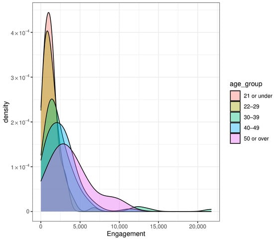
Figure A4.
Density plots of the engagement variable of all age groups.
Before clustering probability distributions, we transformed the data using a density function to obtain the heights of the engagement variable in each age group. For that purpose, the same X values were considered to evaluate the heights of the distributions at the same points. We determined that the Hellinger distance was appropriate to evaluate the dissimilarity between the distributions of students’ age groups. Then, we used a hierarchical clustering method based on Ward’s method to interpret the results shown in Figure A5.
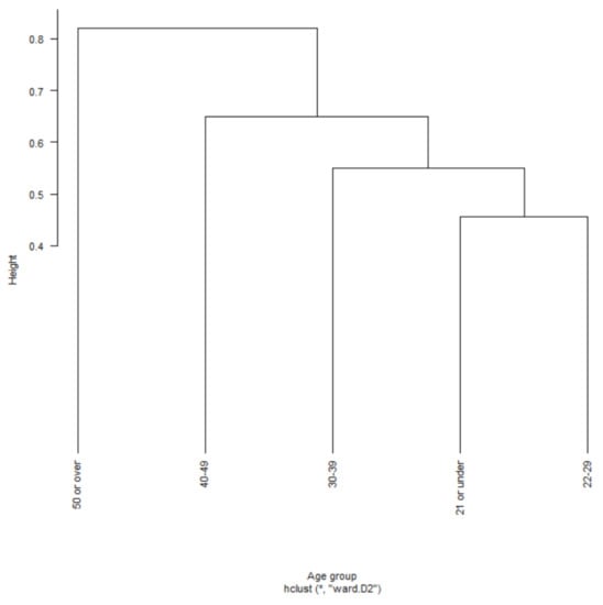
Figure A5.
Dendrogram of the engagement variable of all age groups.
The dendrogram in Figure A5 shows 5 distinctive groups. Those labelled “21 or under” and “22–29” are closely related. However, “30–39”, “40–49”, and “50 or older” show slight differences. Based on the results, there are 4 potential cluster groups that are distinctive in terms of different engagement levels per age-group category. Our analysis and results in Figure A5 show that students from certain age groups have varying levels of engagement with their online program. The proposed method, thus, seems instrumental in analyzing data from online learning platforms.
References
- Brown, B. Delphi Process: A Methodology Used for the Elicitation of Opinions of Experts; Document No: P-3925; RAND: Santa Monica, CA, USA, 1968; 15p. [Google Scholar]
- Barrera-Causil, C.J.; Correa, J.C.; Marmolejo-Ramos, F. Experimental Investigation on the Elicitation of Subjective Distributions. Front. Psychol. 2019, 10, 862. [Google Scholar] [CrossRef]
- Nielsen, F.; Nock, R.; Amari, S.I. On Clustering Histograms with k-Means by Using Mixed α-Divergences. Entropy 2014, 16, 3273–3301. [Google Scholar] [CrossRef]
- Henderson, K.; Gallagher, B.; Eliassi-rad, T. EP-MEANS: An Efficient Nonparametric Clustering of Empirical Probability Distributions. In Proceedings of the 30th Annual ACM Symposium on Applied Computing, Salamanca, Spain, 13–17 April 2015; ACM: New York, NY, USA, 2015. [Google Scholar]
- Wang, J.L.; Chiou, J.M.; Müller, H.G. Review of functional data analysis. Annu. Rev. Stat. Appl. 2016, 3, 257–295. [Google Scholar] [CrossRef]
- Ferreira, L.; Hitchcock, D. A comparison of hierarchical methods for clustering functional data. Commun. Stat. Simul. Comput. 2009, 38, 1925–1949. [Google Scholar] [CrossRef]
- Abraham, C.; Cornillon, P.A.; Matzner-Lober, E.; Molinari, N. Unsupervised Curve Clustering Using B-Splines. Scand. J. Stat. 2003, 30, 581–595. [Google Scholar] [CrossRef]
- Gareth, M.; Sugar, C. Clustering for Sparsely Sampled Functional Data. J. Am. Stat. Assoc. 2003, 98, 397–408. [Google Scholar]
- Serban, N.; Wasserman, L. CATS: Clustering after Transformation and Smoothing. J. Am. Stat. Assoc. 2005, 100, 990–999. [Google Scholar] [CrossRef]
- Shubhankar, R.; Bani, M. Functional Clustering by Bayesian Wavelet Methods. J. R. Stat. Soc. Ser. B (Stat. Methodol.) 2006, 68, 305–332. [Google Scholar]
- Song, J.; Lee, H.; Jeffrey, S.M.; Kang, S. Clustering of time-course gene expression data using functional data analysis. Comput. Biol. Chem. 2007, 31, 265–274. [Google Scholar] [CrossRef]
- Chiou, J.M.; Li, P.L. Functional Clustering and Identifying Substructures of Longitudinal Data. J. R. Stat. Soc. Ser. B (Stat. Methodol.) 2007, 69, 679–699. [Google Scholar] [CrossRef]
- Tarpey, T. Linear Transformations and the k-Means Clustering Algorithm: Applications to Clustering Curves. Am. Stat. 2007, 61, 34–40. [Google Scholar] [CrossRef] [PubMed]
- Goia, A.; May, C.; Fusai, G. Functional clustering and linear regression for peak load forecasting. Int. J. Forecast. 2010, 26, 700–711. [Google Scholar] [CrossRef]
- Hébrail, G.; Hugueney, B.; Lechevallier, Y.; Rossi, F. Exploratory analysis of functional data via clustering and optimal segmentation. Neurocomputing 2010, 73, 1125–1141. [Google Scholar] [CrossRef]
- Boullé, M. Functional data clustering via piecewise constant nonparametric density estimation. Pattern Recognit. 2012, 45, 4389–4401. [Google Scholar] [CrossRef]
- Secchi, P.; Vantini, S.; Vitelli, V. Bagging Voronoi classifiers for clustering spatial functional data. Int. J. Appl. Earth Obs. Geoinf. 2012, 22, 53–64. [Google Scholar] [CrossRef]
- Jacques, J.; Preda, C. Model-based clustering for multivariate functional data. Comput. Stat. Data Anal. 2013, 71, 92–106. [Google Scholar] [CrossRef]
- Jacques, J.; Preda, C. Functional data clustering: A survey. Adv. Data Anal. Classif. 2014, 8, 231–255. [Google Scholar] [CrossRef]
- Stefan, A.; Katsimpokis, D.; Gronau, Q.F.; Wagenmakers, E. Expert agreement in prior elicitation and its effects on bayesian inference. PsyArXiv 2021. [Google Scholar] [CrossRef]
- Simpson, D.G. Minimum Hellinger Distance Estimation for the Analysis of Count Data. J. Am. Stat. Assoc. 1987, 82, 802–807. [Google Scholar] [CrossRef]
- Kahraman, C.; Onar, S.C.; Oztaysi, B. Fuzzy Multicriteria Decision-Making: A Literature Review. Int. J. Comput. Intell. Syst. 2015, 8, 637–666. [Google Scholar] [CrossRef]
- R Core Team. R: A Language and Environment for Statistical Computing; R Foundation for Statistical Computing: Vienna, Austria, 2020. [Google Scholar]
- Febrero-Bande, M.; Oviedo, M. Statistical Computing in Functional Data Analysis: The R Package fda.usc. J. Stat. Softw. 2012, 51, 1–28. [Google Scholar] [CrossRef]
- Maechler, M.; Rousseeuw, P.; Struyf, A.; Hubert, M.; Hornik, K. Cluster: Cluster Analysis Basics and Extensions; R Package Version 2.0.3; R Foundation: Vienna, Austria, 2015. [Google Scholar]
- Hubert, L.; Arabie, P. Comparing partitions. J. Classif. 1985, 2, 193–218. [Google Scholar] [CrossRef]
- Morlini, I.; Zani, S. Dissimilarity and similarity measures for comparing dendrograms and their applications. Adv. Data Anal. Classif. 2012, 6, 85–105. [Google Scholar] [CrossRef]
- Steegen, S.; Tuerlinckx, F.; Gelman, A.; Vanpaemel, W. Increasing Transparency Through a Multiverse Analysis. Perspect. Psychol. Sci. 2016, 5, 702–712. [Google Scholar] [CrossRef]
- Ramsay, J.; Hooker, G.; Graves, S. Functional Data Analysis with R and MATLAB; Springer: Berlin/Heidelberg, Germany, 2009. [Google Scholar]
- Kaufman, L.; Rousseeuw, P. Finding Groups in Data: An Introduction to Cluster Analysis, 1st ed.; Series in Probability and Statistics; Wiley: Hoboken, NJ, USA, 1990. [Google Scholar]
- Nieweglowski, L. clv: Cluster Validation Techniques; R Package Version 0.3-2.1; R Foundation: Vienna, Austria, 2013. [Google Scholar]
- Barrera, C.; Correa, J. Distribución Predictiva Bayesiana Para Modelos de Pruebas de Vida vía MCMC. Ph.D. Thesis, Universidad Nacional de Colombia Sede Medellín, Medellín, Colombia, 2008. [Google Scholar]
- Shanker, R.; Shukla, K.; Shanker, R.; Leonida, T. On modeling of lifetime data using two-parameter Gamma and Weibull distributions. Biom. Biostat. Int. J. 2016, 4, 201–206. [Google Scholar] [CrossRef]
- Rigby, R.A.; Stasinopoulos, M.D. Generalized additive models for location, scale and shape. J. R. Stat. Soc. Ser. C (Appl. Stat.) 2005, 54, 507–554. [Google Scholar] [CrossRef]
- VerMilyea, M.; Hall, J.; Diakiw, S.; Johnston, A.; Nguyen, T.; Perugini, D.; Miller, A.; Picou, A.; Murphy, A.; Perugini, M. Development of an artificial intelligence-based assessment model for prediction of embryo viability using static images captured by optical light microscopy during IVF. Hum. Reprod. 2020, 4, 770–784. [Google Scholar] [CrossRef]
- Arpaci, I.; Alshehabi, S.; Al-Emran, M.; Khasawneh, M.; Mahariq, I.; Abdeljawad, T.; Hassanien, A. Analysis of twitter data using evolutionary clustering during the COVID-19 Pandemic. Comput. Mater. Contin. 2020, 1, 193–204. [Google Scholar] [CrossRef]
- Sinha, A.; Zhao, H. Incorporating domain knowledge into data mining classifiers: An application in indirect lending. Decis. Support Syst. 2008, 46, 287–299. [Google Scholar] [CrossRef]
- Micallef, L.; Sundin, I.; Marttinen, P.; Ammad-ud din, M.; Peltola, T.; Soare, M.; Jacucci, G.; Kaski, S. Interactive elicitation of knowledge on feature relevance improves predictions in small data sets. In Proceedings of the 22nd International Conference on Intelligent User Interfaces, Limassol, Cyprus, 13–16 March 2017; ACM Press: New York, NY, USA, 2017. [Google Scholar]
- Daee, P.; Peltola, T.; Soare, M.; Kaski, S. Knowledge elicitation via sequential probabilistic inference for high-dimensional prediction. Mach. Learn. 2017, 1599–1620. [Google Scholar] [CrossRef]
- Groznik, V.; Guid, M.; Sadikov, A.; Možina, M.; Georgiev, D.; Kragelj, V.; Ribarič, S.; Pirtošek, Z.; Bratko, I. Elicitation of neurological knowledge with argument-based machine learning. Artif. Intell. Med. 2013, 106, 133–144. [Google Scholar] [CrossRef] [PubMed]
- Ramsay, J.; Silverman, B. Functional Data Analysis, 2nd ed.; Springer: New York, NY, USA, 2005. [Google Scholar]
- Giraldo, R. Geostatiscal Analysis of Functional Data. Ph.D. Thesis, Universitat Politécnica de Catalunya, Catalunya, Spain, 2009. [Google Scholar]
- Giraldo, R.; Delicado, P.; Mateu, J. Hierarchical clustering of spatially correlated functional data. Stat. Neerl. 2012, 66, 403–421. [Google Scholar] [CrossRef]
- Cohen-addad, V.; Kanade, V.; Mallmann-trenn, F.; Mathieu, C. Hierarchical Clustering: Objective Functions and Algorithms. J. ACM 2019, 66, 1–42. [Google Scholar] [CrossRef]
- Stone, C. View of online learning in australian higher education: Opportunities, challenges and transformations. Stud. Success 2019, 10, 1–11. [Google Scholar] [CrossRef]
- Devlin, M. The Typical University Student is no Longer 18, Middle-Class and on Campus. We Need to Change Thinking on “Drop-Outs”. 2017. Available online: http://theconversation.com/the-typical-university-student-is-no-longer-18-middle-class-and-on-campus-we-need-to-change-thinking-on-drop-outs-73509 (accessed on 22 November 2019).
Publisher’s Note: MDPI stays neutral with regard to jurisdictional claims in published maps and institutional affiliations. |
© 2021 by the authors. Licensee MDPI, Basel, Switzerland. This article is an open access article distributed under the terms and conditions of the Creative Commons Attribution (CC BY) license (http://creativecommons.org/licenses/by/4.0/).