Abstract
Approximate Bayesian computation is a likelihood-free inference method which relies on comparing model realisations to observed data with informative distance measures. We obtain functional data that are not only subject to noise along their y axis but also to a random warping along their x axis, which we refer to as the time axis. Conventional distances on functions, such as the L2 distance, are not informative under these conditions. The Fisher–Rao metric, previously generalised from the space of probability distributions to the space of functions, is an ideal objective function for aligning one function to another by warping the time axis. We assess the usefulness of alignment with the Fisher–Rao metric for approximate Bayesian computation with four examples: two simulation examples, an example about passenger flow at an international airport, and an example of hydrological flow modelling. We find that the Fisher–Rao metric works well as the objective function to minimise for alignment; however, once the functions are aligned, it is not necessarily the most informative distance for inference. This means that likelihood-free inference may require two distances: one for alignment and one for parameter inference.
1. Introduction
In statistical problems, what constitutes the sample space is sometimes a matter of perspective. One perspective is that the data comprise a set of functions rather than simply numbers [1]. For instance, using ultraviolet-visible spectroscopy, suppose we record the absorbance for a series of samples over a wide range of frequencies. We might regard the sample number and frequency as explanatory variables and absorbance as the response variable; alternatively, for each sample, we could consider the entire functional form of the absorption spectrum as the response variable, in which case the only explanatory variable is the sample number. The sample space could comprise the output range of the machine (a subset of the real line) or the function space of the set of all possible spectra. Functional data analysis (FDA) proceeds with this latter approach [2,3]; these data are termed functional data.
A familiar problem when analysing functional data is misalignment [4,5,6], where there is difficultly comparing observations or deriving meaningful statistics, since the features of the functions do not correspond with one another on the domain. We refer to the domain, by convention, as the time axis, since we consider only functions mapping a bounded subset of to . A simple example of issues with misalignment is the comparison of handwriting samples—if the samples are not on top of each other, then it is difficult to compare them [7].
In cases with misaligned data, it is often helpful to align the functions before proceeding with standard statistical analysis. Standard statistical methods assume that only the amplitude of a function is subject to noise. However, it is possible that the time axis itself is subject to noise in a way that preserves the ordering of observations (warping). The fact that the time axis is warped creates misalignment between the functions. This situation can be elegantly described as a combination of amplitude and phase variation within a functional dataset [7,8].
Dynamic time warping [9,10] and curve registration [11,12] are equivalent terms used in the engineering and statistical literature (respectively), for aligning functions by warping the time axis. Applications of curve registration include alignment of growth curves to improve the usefulness of statistical summaries [13] and alignment of medical equipment signals to optimise surgical workflow [14]. In this paper, we use curve registration to align the data.
In curve registration, an elastic distance between functions displaying both amplitude and phase variation is used. The elastic distance we adopt has mathematically convenient properties [11]. This elastic distance generalises the Fisher–Rao metric [15,16] from the space of probability density functions to the space of absolutely continuous functions. This is referred to as the generalised Fisher–Rao metric (FR).
Parameter inference with functional data is developed under many different names, including self-modelling [17], functional-modelling [3] and longitudinal data analysis [18]. However, these methods require that the likelihood function can be evaluated. In many statistical models, the likelihood function is either unavailable or intractable, but it is possible to draw realisations from the model conditional on parameter values. One approach to parameter inference in these situations is approximate Bayesian computation (ABC). ABC is a likelihood-free approach to parameter inference where the proposed parameter values are accepted when a distance between model realisations and observed data is smaller than some threshold [19].
In ABC, the distance metric employed is usually defined as the Euclidean distance between summary statistics of the observed data and the model realisation. The summary statistics can be obtained in a variety of ways. For instance, one can compute summary statistics based on increments at each step [20], one could use wavelet compression to transform functional data into low-dimensional summary statistics [21] or they could be transformed into estimators for parameters from an autoregressive model [22]. Choosing the most effective summary statistics is problem specific, and might also be dataset-specific [23]. In recent work, summary statistics have been replaced by estimators for metrics on probability measures, such as the Wasserstein distance [24], maximum mean discrepancy (MMD) [25], and the Fisher–Rao metric [26]. These estimators have been used within ABC samplers [24,27]. We compare the FR and the MMD for the purposes of ABC, however, in all cases, the curve registration is itself performed using the FR.
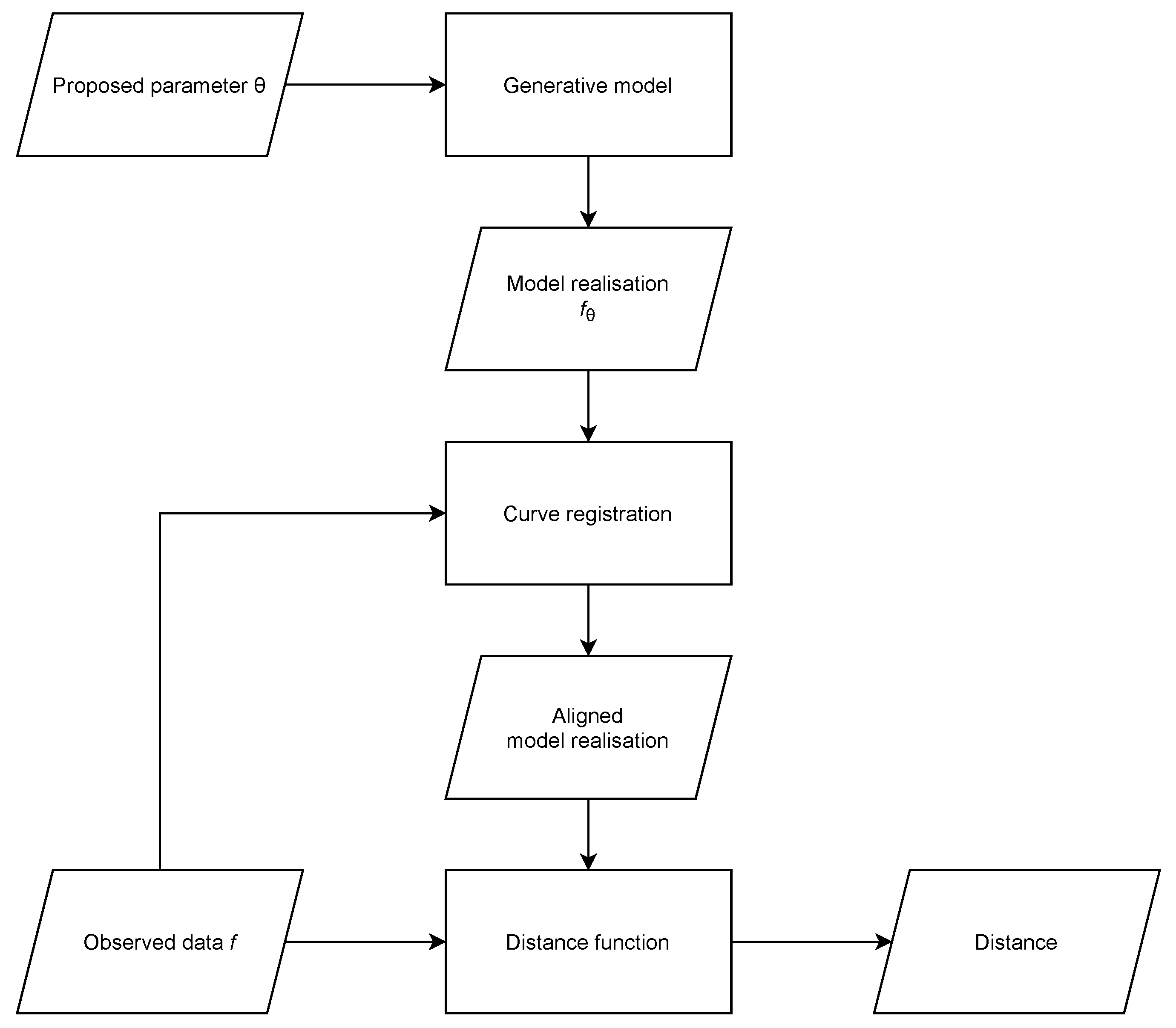
In this paper, we consider problems where the likelihood function is unavailable and the shape and characteristics of the response variables’ functional form encode important information for parameter inference, considering that this functional form is subject to variation in peak locations, which can be modelled as a stochastic warping of the time axis. We incorporate curve registration into the distance computation of ABC (Figure 1).

Figure 1.
Flowchart showing how curve registration is incorporated into distance computation for ABC. This is a diagrammatic representation of Algorithm 2.
In the following Section, we provide some background to functional data analysis and the use of curve registration as well as describing the Fisher–Rao metric and introducing notation. In Section 3, we take a closer look at approximate Bayesian computation and introduce a distance sampler as well as relevant notation. Our approach combining curve registration and ABC is demonstrated with four examples; two simulation examples with random distributions that shift position of peaks, where we test whether ABC with alignment outperforms ABC without alignment (Section 4); a model of passenger flow in an international airport, where we use an algorithm for queueing-based simulation using data consisting of records of passenger numbers passing through specific checkpoints for each minute of the day (Section 5); and a hydrological model, where water flows within catchment areas in response to for example rainfall are forecasted using the GR4J simulation model (Section 6). In Section 7 we summarize our results and conclude with our findings.
2. Functional Data Analysis and Curve Registration
Functional data analysis (FDA), in which datapoints are functions, is a well-established field of study [3]. Special cases of functional data include longitudinal data and time series; however, the field of FDA is much broader [28]. For simplicity, we consider problems in which the functional data comprise a single functional random variable . These variables take values in a function space with probability measure p [29]. In practice, is not directly observed; instead, we observe an empirical function f, with error, on a finite subset of the domain. This is referred to as an empirical functional random variable (EFRV). An EFRV f is a set of pairs , representing the sampling location and corresponding function output . We append the superscript f to associate each EFRV with its sampling points and functional outputs. The set of all sampling locations for f is , similarly is the set of all functional outputs.
When analysing functional data, estimating the mean function is often of interest. In the case of multiple EFRVs , which share the same sampling locations , a standard estimator is , with . In many cases, however, it is possible that the resulting function does not lie within due to misalignment caused by time warping (phase variation). For instance, if is the set of Gaussian functions with and , then the mean function is not a Gaussian function on the time axis.
The functional data can be aligned using curve registration. We assume that is the space of real-valued functions defined on the interval , for some . Curve registration aligns elements of with increasing and invertible automorphisms on the time axis. These automorphisms are called warping functions , such that elements of the set have aligned features according to some criteria. We adopt the elastic functions approach of Srivastava et al. (2011) [11], who align to another functional random variable using the generalised Fisher–Rao (FR) metric:
as the objective function, where . Curve is aligned to by finding the value of which minimises . Since this distance takes phase variation into account, it is called an elastic distance. One advantage of using for curve registration is that:
in other words, the FR is invariant with respect to shared warpings. This implies that the distance of amplitudes between and , defined as
is symmetric [11]. The R package fdasrvf [30], which we use, implements this approach. Since is not directly observed (rather, the EFRV f is observed), a cubic spline approximation to is used to compute the FR distance.
3. Approximate Bayesian Computation
Suppose it is possible to draw samples x from a probability distribution , but it is not possible to directly evaluate for a particular x. Furthermore, suppose we wish to perform inference on . In such cases, so-called likelihood-free approaches are necessary; a popular approach is approximate Bayesian computation (ABC).
The theoretical foundation of ABC rests on the fact that, if we draw samples independently of the prior and use each to generate a corresponding model realisation from , then the set is distributed as . Such an approach would never work in practice, as the proportion of samples equal to x for models with continuous support is generally zero. For this reason, a distance d between x and is used as a decision rule to accept or reject . In other words, we sample the set for some fixed threshold . We should say dissimilarity [31], rather than distance, since, for ABC, a weaker notion than distance is needed, without the triangle inequality and where is true, but the converse is not true in general.
The FR (Equation (1)) is a distance metric for functions. Another distance, which we use, is the estimator for maximum mean discrepancy (), a non-parametric two-sample statistic for testing whether samples come from the same distribution [32]. This has previously been used as a distance within an ABC sampler [27,33]. In this paper, inputs to distances are EFRV. For the purposes of defining we denote these inputs as f and g; however, when used within the d-sampler, one is the observed data f and the other is the model realisation . The definition of is as follows:
where k is some kernel function. The kernel function that we use in this paper is the Gaussian kernel, , where S is a fixed tuning covariance matrix. This distance, , is equivalent to a kernel-smoothed L2 metric between EFRVs [25]. Therefore, we use as a distance on EFRVs rather than probability measures.
Many varieties of ABC samplers exist in the literature, including accept-reject [34], replenishment [35], and simulated annealing [36]. We find it useful in this paper to introduce an additional notion called a distance sampler (d-sampler) (Algorithm 1), which helps to simplify the language used later. The d-sampler is simply the distance viewed as a random variable, which is conditional on , and observed functional data f.
| Algorithm 1 d-sampler. |
|
This notion makes ABC samplers easier to describe. For instance, the rejection sampler can be written as a loop over i with keeping only pairs with less than . In this paper, we adopt the replenishment ABC sampler [35].
To develop an ABC sampler for functional data, we develop d-samplers on and f. We align a model realisation to f with a warping [11], as discussed in the previous Section. The distance between f and the aligned model realisation is computed with either the FR or MMD, as is shown in Algorithm 2. In the next section, we compare these d-samplers against their unregistered versions (Algorithm 1) for two simulation examples of shifting peaks.
| Algorithm 2 Registered d-sampler. |
|
4. Peak Shift
4.1. Methods
To demonstrate our method, we construct two simulation examples. The functional data of the examples are a set of peaks with shifting positions. We test whether ABC with alignment (alignment of f with before distance computation) outperforms ABC without alignment. The first example is as follows: the mean function is a sum over five Gaussian density functions and four Cauchy density functions C, i.e., . This is related to peaks in the spectroscopy, which are either Gaussian or Cauchy (Lorentzian) peaks [37]. The observed functional output corresponding to fixed sampling locations , is independent and normally distributed , conditional on the time axis value and peak positions . What makes this problem of interest is that the location parameters are nuisance parameters, treated as random effects to be integrated out. Instead of integration, we use curve registration to produce a distance which is invariant with respect to , the nuisance parameters. These have distribution for known values for and . The fact that is random and high-dimensional makes inelastic distances, such as the L distance, inappropriate.
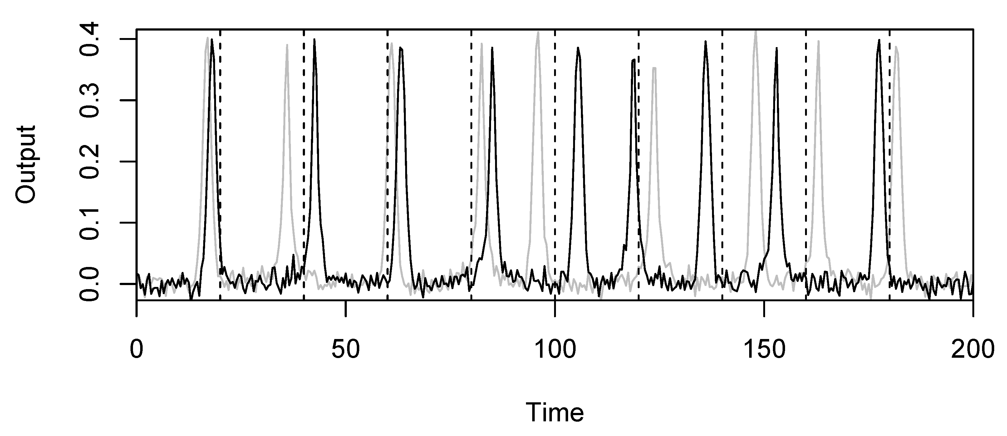
The prior distributions for the parameters of interest are , and . An example of a model realisation from this distribution is shown in Figure 2. To test the effectiveness of registered d-samplers in this situation, we compare all four combinations: MMD and FR with and without registration. We set the covariance matrix S for MMD as the diagonal matrix with elements 9 and . These values within S were chosen based on the scale of the data (see Figure 2).
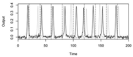
Figure 2.
Example of model realisations from the peak shift model with , and . The dotted lines are the fixed values. The distribution of peak shifts is controlled by , the peak widths are controlled by , and the noise is controlled by .
The second simulation example that we construct is similar to the first, except we use a set of skewed normal density functions SN [38]. The purpose of this example is to further test the robustness of our technique. The mean function here is , where is the scale parameter and is the skewness parameter. This is called the centred parameterisation [39]. The prior distributions for the parameters of interest are , , and .
4.2. Results
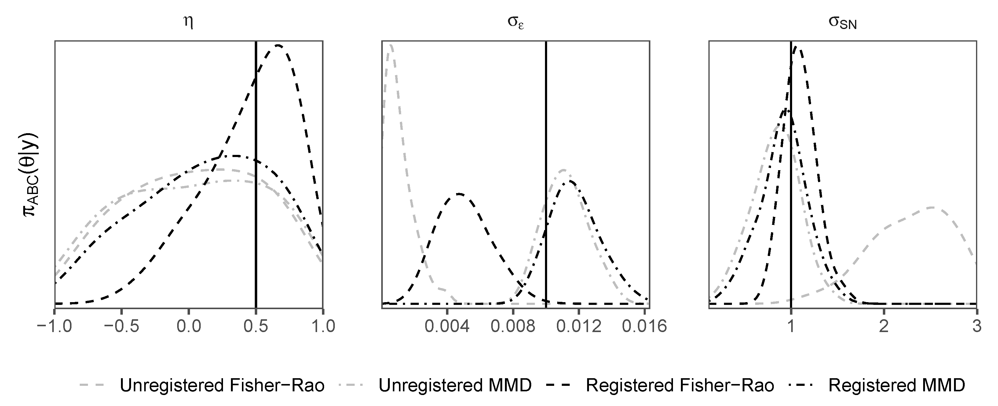
Density plots of posterior samples arising from the ABC sampler with all four d-samplers, registered and unregistered, are shown for the first example in Figure 3 and the second example in Figure 4. The plots show that the registered d-samplers outperform their unregistered counterparts; although the FR is an ideal distance for alignment of functions, when used as a distance for ABC, it is sometimes outperformed by MMD. This suggests that the best distance for registration is not always the best distance for ABC. The reason that MMD outperforms the FR for is its penalty term. The first term in Equation (2) penalises the concentration of , such that the algorithm tends towards a higher value of to match the noise in . The same pattern of density plots is seen between the two examples, with the registered distances outperforming others for peak shape parameters (, and ), and the MMD distance (both registered and unregistered) outperforms the Fisher–Rao distance for the noise parameter .
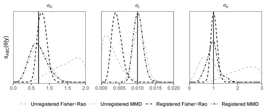
Figure 3.
Gaussian/Cauchy peak shift example. Density plots of posterior samples arising from the replenishment ABC sampler. Distances shown include maximum mean discrepancy (MMD) and Fisher–Rao (FR). These distances are used within the registered (Algorithm 2) and unregistered (Algorithm 1) d-samplers. Vertical black solid lines represent true values.
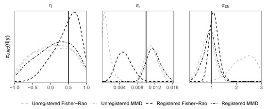
Figure 4.
Skewed Gaussian peak shift example. Density plots of posterior samples arising from the replenishment ABC sampler. Distances shown include maximum mean discrepancy (MMD) and Fisher–Rao (FR). These distances are used within the registered (Algorithm 2) and unregistered (Algorithm 1) d-samplers. Vertical black solid lines represent true values.
The relative merits of each distance are not our primary concern. We are interested in the effect of registration rather than the distance. It is interesting, however, that we can use a different distance for ABC than is used for curve registration and, depending on the parameter of interest, obtain superior results. In further examples, we proceed only with MMD. We now demonstrate a more complex example with a dynamic queueing network model of an international airport terminal.
5. Passenger Processing at an International Airport
Rising demand for air travel and enhanced security screening place pressure on existing airport infrastructure. Airport terminal infrastructure, for financial and geographical reasons, can be difficult to upgrade the rate needed to match this demand. With this in mind, operational planners at airports seek to optimise day-to-day operations. However, optimisation frameworks require models with some degree of realism. These models will necessarily become complicated and this, combined with the data collection scheme, inevitably leads to intractable likelihoods. Simulators are, on the other hand, straightforward to construct, although computationally demanding.
We use a fast algorithm for queueing based simulations, called QDC [40], to construct an ABC sampler for this problem [33]. However, there were problems with misalignment, as noted in their discussion. We consider a simplified (for the sake of exposition) version of this model and data. The purpose of this model is to predict passenger flows through an airport terminal in response to particular flight schedules and staff rosters at an immigration checkpoint. The data comprise records of passenger numbers passing through certain checkpoints for each minute of the day. The flight schedule and staff rosters can be thought of as explanatory variables, since they are known and affect the response variable (passenger flows) to some degree, which we wish to estimate.
We model the arrivals terminal of an international airport. For one day, we have a list of flights u along with their arrival gate and arrival time . The walking distance from gate to immigration is also known. The flight arrival information , collectively, are a type of forcing data; in other words, they are inputs to a simulation model which are themselves subject to observational error [41]. The time that a flight arrives is known, but the time at which a flight opens its doors to deplane passengers is not recorded [33]. This leads to more uncertainty regarding the dynamics of passenger processing. It is of interest whether curve registration helps to improve parameter inference under these conditions.
5.1. Methods
To model passenger flows, we simulate every passenger from every flight. The time at which passenger v from flight u deplanes is , where is the time taken for the passenger to leave the aircraft and is a nuisance parameter representing an unobserved amount of time taken by the crew after the recorded arrival time to open the doors, letting passengers out. Note that, in this example, plays the same role as from the peak shift example, i.e., that of a high-dimensional latent variable, shifting peaks independently.
Once passengers have deplaned, they walk to be processed at immigration and queue for processing. The times at which customers arrive to the queueing system are , where is the walking time to immigration from the arrival gate. The distribution of is Gamma. This is equivalent to sampling from Gamma and multiplying the result by . We transform these parameters, for interpretability to mean , and variance to mean squared ratio . There are two parallel queueing systems: one for local and one for foreign passengers. The proportion of local passengers on each flight is known and encoded in the Boolean variable . Each queueing system proceeds at a different rate and has a different number of servers which are non-interchangeable. This is an accurate depiction of real systems, including staff and automated systems working in parallel and which cannot be interchanged.
We require a queueing simulator to compute the times at which passengers leave their assigned queueing system (local or foreign). A queueing simulator (QueueSim) is a function which (conditional on arrival times, service times and number of servers) deterministically computes the times at which passengers leave their queueing system (departure times), see [40]. First, we partition the arrival times by ; then, we sample service times . There is a separate rate parameter for the local passengers queue and the foreign passengers queue . The number of servers for each queue is known. The departure times from the queueing systems are , where the variables are written in boldface to denote the full vectors partitioned by nationality, since the movements of each passenger, once queueing begins, are no longer independent. The synthetic data were constructed in the same way so that we could know the true parameter values, which are , , , and . The priors are independent and uniform for all parameters , , , . We bin and by minute to construct EFRVs in the form of histograms and , respectively. The two functional variables and represent, respectively, the input and output of the immigration system.
Considering that variations in flight arrival times significantly affect the dynamics of queues within the immigration system, we cannot register and independently to and , respectively, without introducing modelling error. Our solution here is to “correct” for forcing data uncertainty with reference to the warping function. We, therefore, obtain three different types of posterior samples (registered, unregistered and corrected). Since themselves are not functional data, we refer to these as corrected arrival times and denote them as . We use curve registration to find the warping function from to and apply this to the latent variable , correcting and (Algorithm 3). The type argument encodes whether the d-sampler is unregistered, registered, or corrected. For the registered d-sampler, only the distance on is registered. The corrected d-sampler uses a registered distance on and uses the warping function to correct the input for a more accurate output sample .
| Algorithm 3 Airport d-sampler. |
|
5.2. Results
Density plots of posterior samples for all parameters of interest, for each d-sampler, are shown in Figure 5. We see that the registered d-sampler outperforms the unregistered d-sampler for and , which relates to the walking speed, as well as outperforming the unregistered d-sampler for and is as least as good as the unregistered d-sampler for . Furthermore, we see that applying the correction to the input to the immigration system improves the accuracy of the output since the posterior density for the corrected d-sampler outperforms all others for all parameters. Curve registration therefore helps improve parameter inference under the stated conditions and can even help to improve inference by aligning “correcting” forcing data. Models involving a stochastic transformation from unobserved latent variables may benefit from using this technique.
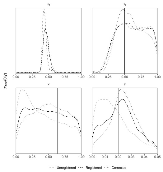
Figure 5.
Density plots of posterior samples using the airport d-sampler (Algorithm 3) for unregistered, registered and corrected types. The solid vertical black line represents the true value. Priors are uniform on the x-axis of each plot.
6. Hydrological Modelling
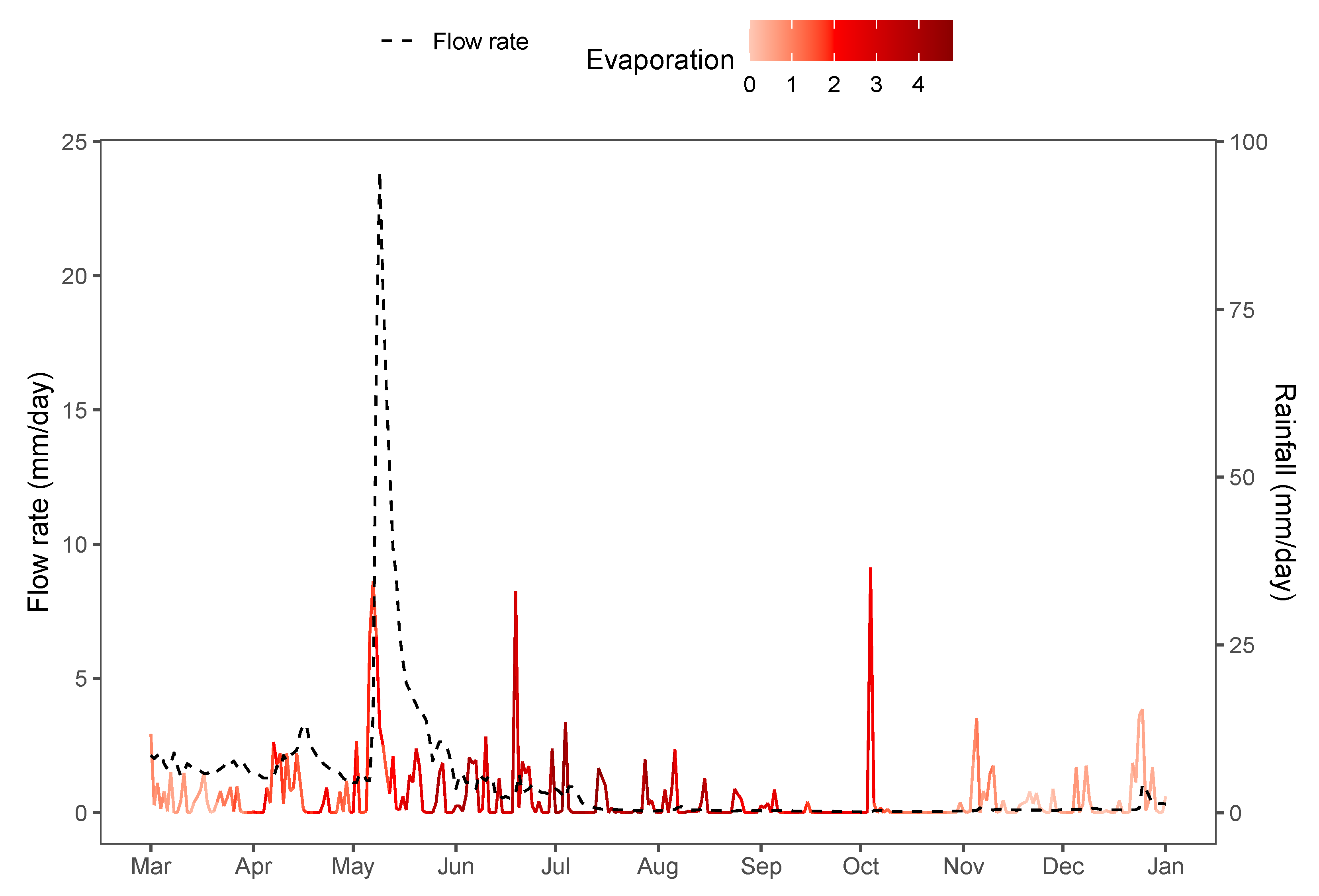
Water flows within catchment areas, in response to rainfall and other weather events, are often modelled and forecast with run-off models, where water flows are represented by hydrographs showing volumetric flow-rates at a particular point (see Figure 6) [42,43]. In particular, the Génie Rural à 4 paramètres Journalier (GR4J) model of [44] is widely used. Parameter estimation for hydrological methods is an active area of research [45]. Once parameters are estimated, parameter uncertainty itself contributes little to overall uncertainty compared to the residual error structure [46].
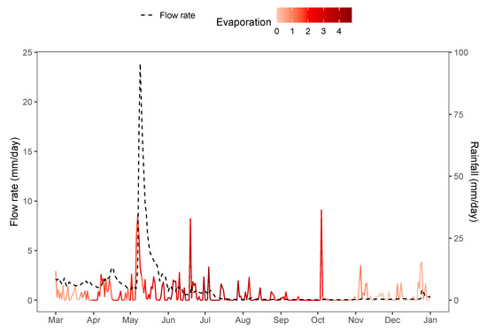
Figure 6.
Synthetic hydrograph with associated rain and evaporation data from the airGR package.
Hydrographs are EFRVs; their functional form is controlled by model parameters and forcing data . For the GR4J model, are rainfall patterns [47]. The peak positions within the functional data are affected by and . However, unlike the airport example, are assumed to be measured without error. As in the previous example, we are interested in whether curve registration helps improve parameter inference.
6.1. Methods
In this example we use the GR4J simulation model. This model contains four parameters: the first three are capacities in units of length (mm); and the fourth parameter () represents a lagged effect in units of time (days). Predictions from the GR4J, given and , are denoted as . As in many run-off models, the GR4J model is deterministic. To provide useful prediction intervals, hydrologists typically add an error structure to the deterministic model. Run-off predictions are positively valued, and errors are heteroscedastic [45]. A common strategy is to perform a Box-Cox transformation of the deterministic output, add noise and then invert the Box-Cox transformation:
The model is an input/output model like the airport example; however, in this case, the input is not a latent variable, but observed directly, so we do not include a corrected d-sampler. We use the same d-samplers used in the peak shift simulation examples (Algorithms 1 and 2).
6.2. Results
As the previous examples, this example includes peak shifting. However, in this case, we see from density plots of posterior samples (Figure 7) that the unregistered d-sampler outperforms the registered d-sampler. In the previous examples, there was a high-dimensional latent variable affecting the peak locations; in this case, there is only one variable affecting the peak locations, i.e., . Since the peak positions shift according to a one-dimensional parameter of interest , rather than a high-dimensional nuisance parameter, the process of registration is unnecessary here, and adds noise to the d-sampler, flattening the posterior densities. Curve registration will therefore not improve parameter inference, since the ABC sampler correctly identifies appropriate values for .
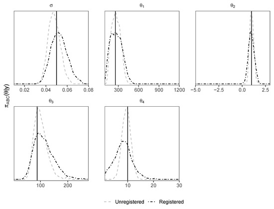
Figure 7.
Density plots of posterior samples from the hydrological model using unregistered and registered d-samplers.
7. Conclusions
In this work, curve registration techniques are applied to the problem of misaligned functional data for likelihood-free inference for the first time. Interested readers can find the code we used at https://github.com/AnthonyEbert/CurveRegistration, accessed on 3 September 2021. We used the FR as an objective function to align model realisations to observed data by warping the time axis. Once functional data were aligned, we compared the FR and MMD as distances for posterior inference within an ABC sampler. We tested this approach with four examples: two peak shift examples (Section 4), the airport example (Section 5), and a real hydrology example (Section 6). The examples highlight different aspects and use-cases of applying curve registration techniques to ABC.
In the peak shift examples of Section 4, we found that the registered d-samplers based on both the FR and MMD outperform the unregistered d-samplers, although the MMD, in some cases, outperformed FR. This means that the distance for alignment is not necessarily the best distance for ABC samplers once alignment is performed. In the airport example of Section 5, we explored the effect of stochasticity in forcing data affecting peak positions. We found that ABC inference based on curve registered functional data increased posterior concentration near the true value. Furthermore, we found that we can “correct” , a latent variable computed within the model itself, by using the warping function computed from the original alignment. This further improves posterior inference, counteracting the effect of forcing data uncertainty. Finally, in the hydrological example (Section 6), the ABC sampler correctly identifies appropriate values for , making curve registration unnecessary in this example; when peak location stochasticity is entirely controlled by parameters of interest, then curve registration ceases to improve posterior inference for those parameters.
While the Fisher–Rao metric is an exceedingly appropriate distance for curve registration, in these cases, it was not necessarily the best distance to use for approximate Bayesian computation (ABC). This means that two distances may be ideal for different purposes within an ABC sampler.
ABC samplers suffer in high dimensions; therefore, the purpose of curve registration is to build distances which are invariant with respect to certain types of high-dimensional nuisance parameters. We find, illustrated by the four examples, that curve registration provides a valuable technique for posterior inference based on misaligned functional data, where variation in peak positions is controlled by nuisance parameters.
Author Contributions
Conceptualization, A.E., K.M., F.R. and P.W.; methodology, A.E., K.M., F.R. and P.W.; software, A.E.; validation, A.E. and P.W.; formal analysis, A.E.; investigation, A.E.; resources, A.E., K.M. and P.W.; data curation, A.E.; writing—original draft preparation, A.E.; writing—review and editing, A.E. and F.R.; visualization, A.E. and F.R.; supervision, K.M., F.R. and P.W.; project administration, K.M.; funding acquisition, K.M. and P.W. All authors have read and agreed to the published version of the manuscript.
Funding
This work was supported by the ARC Centre of Excellence for Mathematical and Statistical Frontiers (ACEMS). This work was funded through the ARC Linkage Grant “Improving the Productivity and Efficiency of Australian Airports” (LP140100282).
Institutional Review Board Statement
Not applicable.
Informed Consent Statement
Not applicable.
Data Availability Statement
Data and code to simulate and analyse data are available at https://github.com/AnthonyEbert/CurveRegistration (accessed on 1 June 2021).
Acknowledgments
The authors wish to acknowledge the support of the Queensland University of Technology High Performance Computing and Research Group (HPC). The authors wish to thank Elisabeth Ankersen for proofreading the manuscript.
Conflicts of Interest
The authors declare no conflict of interest.
References
- Thapa, S.; Lomholt, M.A.; Krog, J.; Cherstvy, A.G.; Metzler, R. Bayesian nested sampling analysis of single particle tracking data: Maximum likelihood model selection applied to stochastic diffusivity data. Phys. Chem. Chem. Phys. 2018, 20, 29018–29037. [Google Scholar] [CrossRef]
- Hsing, T.; Eubank, R. Theoretical Foundations of Functional Data Analysis, with an Introduction to Linear Operators; Wiley: New York, NY, USA, 2015. [Google Scholar]
- Ramsay, J.O. Functional Data Analysis; Springer: New York, NY, USA, 2006. [Google Scholar]
- De La Casinière, A.; Cabot, T.; Touré, M.L.; Masserot, D.; Lenoble, J. Method for correcting the wavelength misalignment in measured ultraviolet spectra. Appl. Opt. 2001, 40, 6130–6135. [Google Scholar] [CrossRef] [PubMed]
- Pigoli, D.; Hadjipantelis, P.Z.; Coleman, J.S.; Aston, J.A. The statistical analysis of acoustic phonetic data: Exploring differences between spoken Romance languages. J. R. Stat. Soc. Ser. C Appl. Stat. 2018, 67, 1103–1145. [Google Scholar] [CrossRef]
- Wu, W.; Hatsopoulos, N.G.; Srivastava, A. Introduction to neural spike train data for phase-amplitude analysis. Electron. J. Stat. 2014, 8, 1759–1768. [Google Scholar] [CrossRef]
- Kneip, A.; Ramsay, J.O. Combining registration and fitting for functional models. J. Am. Stat. Assoc. 2008, 103, 1155–1165. [Google Scholar] [CrossRef]
- Srivastava, A.; Klassen, E.P. Functional and Shape Data Analysis; Springer: New York, NY, USA, 2016. [Google Scholar]
- Wang, K.; Gasser, T. Alignment of curves by dynamic time warping. Ann. Stat. 1997, 25, 1251–1276. [Google Scholar] [CrossRef]
- Itakura, F. Minimum prediction residual principle applied to speech recognition. IEEE Trans. Acoust. Speech, Signal Process. 1975, 23, 67–72. [Google Scholar] [CrossRef]
- Srivastava, A.; Wu, W.; Kurtek, S.; Klassen, E.P.; Marron, J.S. Registration of functional data using Fisher-Rao metric. arXiv 2011, arXiv:1103.3817. [Google Scholar]
- Marron, J.S.; Ramsay, J.O.; Sangalli, L.M.; Srivastava, A. Statistics of time warpings and phase variations. Electron. J. Stat. 2014, 8, 1697–1702. [Google Scholar] [CrossRef] [Green Version]
- Cheng, W.; Dryden, I.L.; Huang, X. Bayesian registration of functions and curves. Bayesian Anal. 2016, 11, 447–475. [Google Scholar] [CrossRef]
- Padoy, N.; Blum, T.; Ahmadi, S.A.; Feussner, H.; Berger, M.O.; Navab, N. Statistical modeling and recognition of surgical workflow. Med Image Anal. 2012, 16, 632–641. [Google Scholar] [CrossRef] [PubMed]
- Rao, C.R. Information and the accuracy attainable in the estimation of statistical parameters. Bull. Calcutta Math. Soc. 1945, 37, 81–91. [Google Scholar]
- Maybank, S.J. The Fisher-Rao metric. Math. Today 2008, 44, 255–257. [Google Scholar]
- Kneip, A.; Gasser, T. Convergence and consistency results for self-modeling nonlinear regression. Ann. Stat. 1988, 16, 82–112. [Google Scholar] [CrossRef]
- Laird, N.M.; Ware, J.H. Random-effects models for longitudinal data. Biometrics 1982, 38, 963–974. [Google Scholar] [CrossRef]
- Sisson, S.A.; Fan, Y.; Beaumont, M.A. (Eds.) Handbook of Approximate Bayesian Computation; CRC Press: Boca Raton, FL, USA, 2018. [Google Scholar]
- Cherstvy, A.G.; Thapa, S.; Wagner, C.E.; Metzler, R. Non-Gaussian, non-ergodic, and non-Fickian diffusion of tracers in mucin hydrogels. Soft Matter 2019, 15, 2526–2551. [Google Scholar] [CrossRef]
- Zhu, H.; Lu, R.; Ming, C.; Gupta, A.K.; Müller, R. Estimating parameters in complex systems with functional outputs: A wavelet-based approximate Bayesian computation approach. In New Advances in Statistics and Data Science; Chen, D.-G., Jin, Z., Li, G., Liu, A., Zhao, Y., Eds.; Springer: Berlin, Germany, 2017; pp. 137–160. [Google Scholar]
- Wood, S.N. Statistical inference for noisy nonlinear ecological dynamic systems. Nature 2010, 466, 1102–1104. [Google Scholar] [CrossRef] [Green Version]
- Nunes, M.A.; Balding, D.J. On optimal selection of summary statistics for approximate Bayesian computation. Stat. Appl. Genet. Mol. Biol. 2010, 9, 34. [Google Scholar] [CrossRef]
- Bernton, E.; Jacob, P.E.; Gerber, M.; Robert, C.P. Approximate Bayesian computation with the Wasserstein distance. J. R. Stat. Soc. Ser. B 2019, 81, 235–269. [Google Scholar] [CrossRef]
- Gretton, A.; Borgwardt, K.M.; Rasch, M.J.; Schölkopf, B.; Smola, A. A kernel two-sample test. J. Mach. Learn. Res. 2012, 13, 723–773. [Google Scholar]
- Srivastava, A.; Jermyn, I.; Joshi, S.H. Riemannian analysis of probability density functions with applications in vision. In Proceedings of the IEEE Computer Vision and Pattern Recognition (CVPR), Minneapolis, MN, USA, 17–22 June 2007. [Google Scholar]
- Park, M.; Jitkrittum, W.; Sejdinovic, D. K2-ABC: Approximate Bayesian computation with kernel embeddings. In Proceedings of the 19th International Conference on Artificial Intelligence and Statistics, Cadiz, Spain, 9–11 May 2016. [Google Scholar]
- Wang, J.-L.; Chiou, J.-M.; Müller, H.-G. Functional data analysis. Annu. Rev. Stat. Its Appl. 2016, 3, 257–295. [Google Scholar] [CrossRef] [Green Version]
- Delaigle, A.; Hall, P. Defining probability density for a distribution of random functions. Ann. Stat. 2010, 38, 1171–1193. [Google Scholar] [CrossRef] [Green Version]
- Tucker, J.D. fdasrvf: Elastic Functional Data Analysis. R Package Version 1.9.4. 2020. Available online: https://CRAN.R-project.org/package=fdasrvf (accessed on 22 April 2021).
- Jousselme, A.-L.; Maupin, P. Distances in evidence theory: Comprehensive survey and generalizations. Int. J. Approx. Reason. 2012, 53, 118–145. [Google Scholar] [CrossRef] [Green Version]
- Gretton, A.; Borgwardt, K.M.; Rasch, M.; Schölkopf, B.; Smola, A.J. A kernel method for the two-sample problem. In Advances in Neural Information Processing Systems 19; Schölkopf, B., Platt, J., Hofmann, T., Eds.; MIT Press: Cambridge, MA, USA, 2007; pp. 513–520. [Google Scholar]
- Ebert, A.; Dutta, R.; Mengersen, K.; Mira, A.; Ruggeri, F.; Wu, P. Likelihood-free parameter estimation for dynamic queueing networks: Case study of passenger flow in an international airport terminal. J. R. Stat. Soc. C 2021, 70, 770–792. [Google Scholar] [CrossRef]
- Tavaré, S.; Balding, D.J.; Griffiths, R.C.; Donnelly, P. Inferring coalescence times from DNA sequence data. Genetics 1997, 145, 505–518. [Google Scholar] [CrossRef] [PubMed]
- Drov, I.C.C.; Pettitt, A.N. Estimation of parameters for macroparasite population evolution using approximate Bayesian computation. Biometrics 2011, 67, 225–233. [Google Scholar]
- Albert, C.; Künsch, H.R.; Scheidegger, A. A simulated annealing approach to approximate Bayes computations. Stat. Comput. 2015, 25, 1217–1232. [Google Scholar] [CrossRef] [Green Version]
- Posener, D.W. The shape of spectral lines: Tables of the Voigt profile. Aust. J. Phys. 1959, 12, 184–196. [Google Scholar] [CrossRef]
- Azzalini, A. The skew-normal distribution and related multivariate families. Scand. J. Stat. 2005, 32, 159–188. [Google Scholar] [CrossRef]
- Azzalini, A.; Capitanio, A. Statistical applications of the multivariate skew normal distribution. J. R. Stat. Soc. Ser. B 1999, 61, 579–602. [Google Scholar] [CrossRef]
- Ebert, A.; Wu, P.; Mengersen, K.; Ruggeri, F. Computationally Efficient Simulation of Queues: The R Package queuecomputer. J. Stat. Softw. 2020, 95, 1–29. [Google Scholar] [CrossRef]
- Kavetski, D.; Franks, S.W.; Kuczera, G. Confronting input uncertainty in environmental modelling. In Calibration of Watershed Models 6; Duan, Q., Gupta, H.V., Sorooshian, S., Rousseau, A.N., Turcotte, R., Eds.; Wiley: New York, NY, USA, 2003; pp. 49–68. [Google Scholar]
- Vaze, J.; Chiew, F.H.S.; Perraud, J.-M.; Viney, N.; Post, D.; Teng, J.; Wang, B.; Lerat, J.; Goswami, M. Rainfall-runoff modelling across southeast Australia: Datasets, models and results. Australas. J. Water Resour. 2011, 14, 101–116. [Google Scholar] [CrossRef]
- Harlan, D.; Wangsadipura, M.; Munajat, C.M. Rainfall-runoff modeling of Citarum Hulu River basin by using GR4J. In Proceedings of the World Congress on Engineering 2010, London, UK, 30 June–2 July 2010; Volume II. [Google Scholar]
- Perrin, C.; Michel, C.; Andréassian, V. Improvement of a parsimonious model for streamflow simulation. J. Hydrol. 2003, 279, 275–289. [Google Scholar] [CrossRef]
- Kavetski, D. Parameter estimation and predictive uncertainty quantification in hydrological modelling. In Handbook of Hydrometeorological Ensemble Forecasting; Duan, Q., Pappenberger, F., Wood, A., Cloke, H.L., Schaake, J.C., Eds.; Springer: Berlin, Germany, 2019; pp. 481–522. [Google Scholar]
- McInerney, D.; Thyer, M.; Kavetski, D.; Bennett, B.; Lerat, J.; Gibbs, M.; Kuczera, G. A simplified approach to produce probabilistic hydrological model predictions. Environ. Model. Softw. 2018, 109, 306–314. [Google Scholar] [CrossRef]
- Renard, B.; Kavetski, D.; Leblois, E.; Thyer, M.; Kuczera, G.; Franks, S.W. Toward a reliable decomposition of predictive uncertainty in hydrological modeling: Characterizing rainfall errors using conditional simulation. Water Resour. Res. 2011, 47, W11516. [Google Scholar] [CrossRef]
Publisher’s Note: MDPI stays neutral with regard to jurisdictional claims in published maps and institutional affiliations. |
© 2021 by the authors. Licensee MDPI, Basel, Switzerland. This article is an open access article distributed under the terms and conditions of the Creative Commons Attribution (CC BY) license (https://creativecommons.org/licenses/by/4.0/).

