Article

Learning Time Acceleration in Support Vector Regression: A Case Study in Educational Data Mining

by
Jonatha Sousa Pimentel
1,
Raydonal Ospina
2 and
Anderson Ara
1,*
1
Statistics Department, Federal University of Bahia, Salvador 40170-110, Brazil
2
Statistics Department, CASTLab, Federal University of Pernambuco, Recife 50670-901, Brazil
*
Author to whom correspondence should be addressed.
Stats 2021, 4(3), 682-700; https://doi.org/10.3390/stats4030041
Submission received: 2 July 2021 / Revised: 12 August 2021 / Accepted: 14 August 2021 / Published: 31 August 2021
(This article belongs to the Section Computational Statistics)

Abstract

:
The development of a country involves directly investing in the education of its citizens. Learning analytics/educational data mining (LA/EDM) allows access to big observational structured/unstructured data captured from educational settings and relies mostly on machine learning algorithms to extract useful information. Support vector regression (SVR) is a supervised statistical learning approach that allows modelling and predicts the performance tendency of students to direct strategic plans for the development of high-quality education. In Brazil, performance can be evaluated at the national level using the average grades of a student on their National High School Exams (ENEMs) based on their socioeconomic information and school records. In this paper, we focus on increasing the computational efficiency of SVR applied to ENEM for online requisitions. The results are based on an analysis of a massive data set composed of more than five million observations, and they also indicate computational learning time savings of more than 90%, as well as providing a prediction of performance that is compatible with traditional modeling.

1. Introduction

Education as a human right is a prerequisite for an individual to function fully as a human being in modern society. For instrumental reasons, the guarantee of education as a multi-faceted social, economic and cultural human right allows the development of a society because it facilitates economic self-sufficiency through employment or self-employment and promotes the full development of the human personality. However, in a country such as Brazil, with strong social inequality inherited from a history of slavery, access to education for all as a high-quality public service plays an fundamental role in reducing this inequality. Moreover, equalizing opportunities within education is an even greater challenge. It has long been observed that there are racial discrepancies when it comes to study opportunities. At the end of the 20th century, it had already been observed that the average difference in years of study between white and black individuals was 2 years [1] and actions regarding equality and high-quality education must be connected: they cannot be seen as policy trade-offs [2].
Educational data are increasingly being used to support effective policy and practice and to move education systems towards more evidence-informed approaches to large-scale improvement. Generally, high-income countries with established assessment programmes use data for sector-wide reforms or interventions to improve learning outcomes. Low-income countries that are beginning to use these programmes tend to identify a few separate issues, such as resource allocation, correlations between students’ socio-economic status and their performance, and teacher qualifications. Resulting policies include interventions prompted by demands for policies to address equity issues.
Statistical/machine Learning (ML) based on computer tools and statistical methodologies allows for the semi-automatic discovery of knowledge in LA/EDM by finding patterns and extract useful information from large data sets [3]. LA/EDM, augmented with background data by the use of ML, provide, for example, information on how well students are learning, what factors are associated with achievement, and which groups perform poorly. This information can be used in a predictive framework to evaluate the capacity of systems, improved resource allocation, agenda setting, or during the policy cycle. In this context, the support vector machine or support vector model (SVM) is an ML framework for classification and regression [4] that enables the performance of comprehensive statistical learning and, despite the lack of studies in this field of research, it can be used in LA/EDM. The success of support vector models as machine learning models is based on four main factors [5]: (i) rooted in the statistical learning theory, SVMs possess superior generalization capacity; (ii) a globally optimal solution is obtainable by solving a convex optimization problem, while the problems of local minima impede other contemporary approaches, such as neural networks; (iii) using the so-called kernel trick, it is convenient to solve non-linear problems in arbitrarily high-dimensional feature spaces; (iv) only a part of the training samples are involved in solution representation. Liang et al. [6] used SVM for online courses to predict whether students would drop out in the next ten days. Mite-Baidal et al. [7] presented a literature review using sentiment analysis for educational data mining and indicated that SVM and Naive Bayes are the most used techniques. Pujianto et al. [8] used SVM for text classification for journal articles about Primary School Teacher Education. Ranjeeth et al. [9] used a single SVM and other machine learning models for the prediction of student performance in secondary education. The use of SVR has been less common for educational purposes. López-Martín et al. [10] used SVR with linear kernel to predict the productivity of higher-education graduate students. Indeed, support vector models have been used successfully to solve numerous other complex problems [3], such as flight control [11], security [12], genomics [13], cancer prediction [14,15], facial recognition [16], predicting solar and wind energy resources [17], and predicting academic dropouts [18], among others.
After gathering educational data, the LA/EDM analytical pipeline begins with pre-processing the data that consumes more than 50% of the pipeline and selecting and transforming variables of interest [19,20]. The volume of data generated annually by all students, in a populous country such as Brazil, tends to be enormous; the microdata from the average grades of a student taking their National High School Exams (ENEMs—Exame Nacional do Ensino Médio), held in 2019, contained approximately 5 million observations [21].
Most of the data in the field of learning analytics (LA) and educational data mining (EDM) are characterized by being big data, second-hand, observational, and unstructured [22]. Experiments show that when the training data set is very small, training with auxiliary data can produce significant improvements in accuracy, even when the auxiliary data are significantly different from the training (and test) data. However, in our case, the population of students is very dynamic and the cost of improving accuracy can be very high given the high-dimensional data of the educational data set [23,24,25].
In this study, we focus on improving the computational performance of the learning process with an SVM model in order to predict the average grades of ENEM candidates in Brazil. This process is based on a massive data set that contained the socio-economic characteristics of the exam candidates. Model improvements are required in order to be able to reduce the time needed for learning the native model in large databases. Our approach uses a “Weak SVM” [26] to accelerate the learning procedure in the training regression model step. The remainder of this paper is organized as follows. The preliminaries and the descriptions of the data set are formally given in Section 4. The developed methodology is introduced in Section 2. Section 3 presents a proposed solution to the SVR estimation problem for large databases. The experimental results and the evaluation are given in Section 5. Finally, the conclusions are given in Section 6.

2. Background

With advances in LA/EDM, new meaningful insights can be obtained from large data sets towards helping to identify novel and useful patterns besides predicting the outcome of future observations. The combination of artificial intelligence and data science covers a range of computational approaches and methods towards the extraction of actionable knowledge from large, complex, multidimensional, and diverse data sources. Recently, the use of data mining tools and applied machine learning has risen over conventional statistical approaches for more accurate predictions [3].

2.1. Support Vector Regression

Support vector models are a class of powerful ML methods introduced by Vapnik and co-workers [27,28,29,30] for classification and regression models that often have superior predictive performance to classical neural networks. Their remarkably elegant optimization and risk minimization theories provide robust performance with respect to sparse and noisy data, which makes them the optimal choice in several applications. A support vector machine (SVM) is primarily a method that performs classification tasks by constructing hyperplanes in a multidimensional space that separates cases of different class labels. In many situations where the response variable is continuous, i.e., y R , it is possible to use SVM to predict the outcome by using covariates via a regression model, the so-called support vector regression (SVR) [31]. In this sense, SVMs can handle multiple continuous and categorical variables. To construct an optimal hyperplane, an SVM employs training algorithms, which are used to minimize an error function.
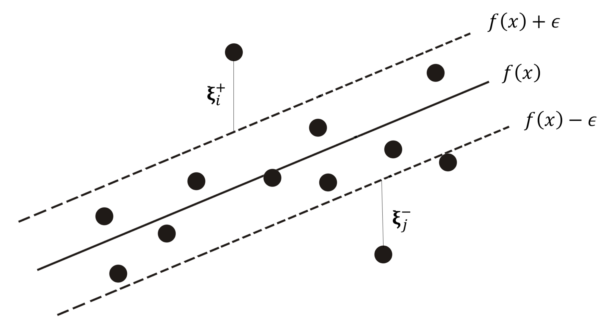
The general idea of support vector models for regression in the linear situation is to build a hyperplane f ( x ) = w x + ϵ = 0 , where x is the vector of the explanatory variables, w is the parameter vector, and ϵ > 0 is a hyperparameter. This representation is plotted in Figure 1, which separates observations within a 2 ϵ wide hyper-tube covering all observations as close as possible to the external limits [32], i.e., margin equations are minimized.
In practical situations, not all observations are expected to be inside this hyper-tube where ϵ is small. In this way, slack variables ξ are added to the linear SVM with smooth margins, so that the model becomes suitable (see plot in Figure 2).
When using slack variables, the optimization problem is based on finding an optimal hyperplane that maximizes the hyper-tube margins and minimizes the slack variable, where we have ξ + for values above the upper margin and ξ for values below the lower margin, and w is the (not necessarily normalized) normal vector to the hyperplane. In general, it is given by the following convex optimization problem:
min 1 2 w , w + C i = 1 n ( ξ i + + ξ i ) ,
where . , . denotes the inner product and C is a regularization constant that imposes a weight on minimizing errors, since there is no limit to the number of incorrect classifications. If C , a smooth-margin SVR returns to a hard-margin SVR. After applying the maximization process via positive Lagrange multipliers α + and α , generated, respectively, by ξ + and ξ , our SVR classifier is given by:
f ( x ) = i = 1 n ( α i + α i ) x i , x 1 n i = 1 n j = 1 n ( α i + α i ) x i , x j y j ,
which only depends on the support vectors. It is also worth mentioning the influence of the sample size on the optimization process used to estimate the parameters of the support vector models. Basically, the larger the size of the data set, the more parameters will be estimated, being directly linked to the number of α s (restrictions) of the model.
The traditional problem with SVM is that it can only find a linear boundary, which is often not possible. The trick is to map the training data or input space ( R ) to a higher-dimensional space called the feature space ( F ) and then use kernel functions to represent the inner product of two data vectors projected onto this space. The mapping is realized via the ϕ function, which is implicitly given by the kernel function. The appropriate choice of the ϕ mapping function or the kernel function implies that the training set mapped in F can be separated by a linear SVM, as shown in Figure 3. The advantage of this approach is that we can implicitly map data onto higher-dimensional space and only inner products are needed to estimate the parameters.
A problem that can be found is the fact that the size of F can be very high, bringing a high computational cost. Replacing the scalar product by means of a kernel function K ( x i , x j ) = ϕ ( x i ) , ϕ ( x j ) is thus straightforward and does not affect the solver. The most used kernel functions are listed in Table 1.
where σ > 0 , d R and q { 2 , 3 , } .
SVM models are highly dependent on a number of user-defined parameters (hyper-parameters); such parameters include: the regularization parameters, the tube size of the ε -insensitive loss function, and the bandwidth of the kernel functions. An inappropriate choice of the parameters may lead to over-fitting or under-fitting [34], and, for massive data problems, this is a troublesome situation.

2.2. SVM Applied to Large Databases

In the traditional method of formulating an SVM, the number of underlying support vectors (SVs) is usually linear with respect to the sample size n , and this implies a high prediction cost, as the standard training procedures to solve the dual problem of kernel SVMs such as Sequential Minimum Optimization (SMO) [35] require Ω ( n ) iterations each with O ( n ) cost [36].
Tsang et al. [37] propose the Core Vector Machine (CVM) algorithm, which, different from the native SVM algorithm, has a time complexity that does not depend on the size of the training sample. Experiments on large data sets, with real and simulated data, have shown that CVM is as accurate as traditional SVM, but it is much faster and can handle larger data sets. This method differs from the native SVM by formulating the kernel method as a minimum enclosing ball (MEB) problem, as well as proposing a specified approximation algorithm to estimate its parameters. From another perspective, Sarmento [38] presented a series of techniques used for the application of SVM in large databases, all focused on the selection of representative samples and, in sequence, the application of the traditional SVM algorithm. Among the suggested methods for sample selection, we can mention the k-nearest neighbors method (KNN) [39], Random Selection Reduction and Convolutional Neural Networks [40]. Applying the suggested methods, results are extracted from synthetic and real data, concluding that the use of such techniques brings good results that reduce the computational cost necessary for the execution of the model. Finally, Torres et al. [41] improved a version of the SMO algorithm for training classification and regression SVMs, based on a Conjugate Descent procedure, decreasing the number of iterations needed for convergence. These cited methods are based on some sophisticated concepts to improve the computational performance, modifying some ideas of the basic theory of SVM. In this paper, we consider a more intuitive concept based on Weak SVR applied to regression tasks. This method is presented in the next section.

3. Reducing Learning Time Using Weak SVMs

To apply SVM models to large data sets, data reduction (reducing the number of support vectors) appears to be priority. Wang et al. [26] present another technical option that reduces the training base for the later use of traditional SVM directed towards classification. In their work, the so-called Weak SVMs are used, which are models adjusted to small databases sampled from the initial base, to carry out the selection of observations and then build a training base smaller than the original base.
A Weak SVR, also known as a ε -Gross Granularity Weak SVR [26], considers X = x 1 , , x n as the training data set, and X ˙ as a subset of X, in which the cardinality of X ˙ is much smaller than X. In other words, X ˙ X , and C a r d ( X ˙ ) < < C a r d ( X ) . In this sense, f ( x ) = w T x subject to | y f ( x ) | < ϵ is the SVR predictor of X as well as f ( x ˙ ) = w ˙ T x ˙ + ϵ is the SVR predictor of X ˙ . The SVR of X ˙ is called the ε -Gross Granularity Weak SVR and its empirical loss function is given by the following equation:
L ( W ˙ , X ˙ ) L ( W , X ) + ε
where L ( W , X ) is the empirical loss function of f ( x ) and ε is a constant.
Though the relationship between the size of the training data set and the bound error ε is weak since the performance of the hypothesis predictor depends on the size of the training data set, Weak SVRs are defined with training data sets with n 0 < < n [26,42].
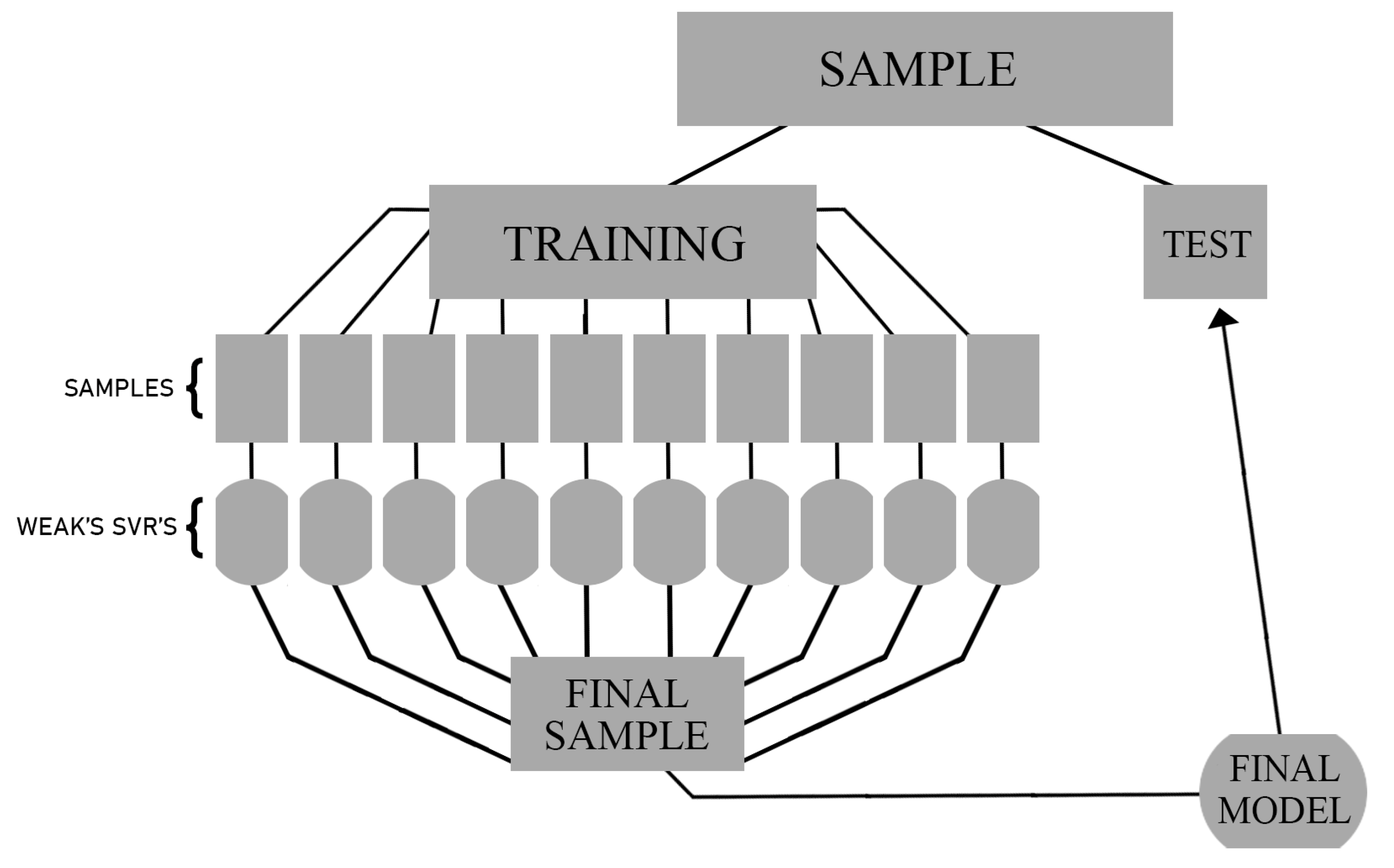
The entire procedure is based on two stages for training data. A random sub-sampling data cleaning method is applied in the first stage, and two maximum entropy-based informative pattern extraction methods are presented in the second stage. In this final constructed base, the traditional SVM model is applied, which has a shorter estimation time, since most of the observations were previously removed. The results achieved by this method are comparable to other methods such as PEGASOS [43], LIBLINEAR [44], and RSVM [45]. In this work, we modify the algorithm proposed by Wang et al. [26] by transforming the SVM algorithm of classification based on Weak SVR for a regression problem and using it for predicting a student’s average grade on the ENEM associated with covariates. In this approach, the variability of the values estimated by “Weak SVR” will be considered instead of the “Weak SVM” proposed by Wang et al. [26]. In other words, this approach considers a regression task to predict a continuous variable instead of the classification task considered in the previous work. Figure 4 shows the flowchart of steps used by the modified method proposed.

3.1. Initial Sampling

The first step in the approach used is to extract K samples of size n 0 < < n from the population, to adjust the K SVR models, which will now be called the “Weak SVRs”. These initial K models are said to be “weak” because they are fitted from a small sample size when compared to the original sample size of the initial base.

3.2. Adjustment and Prediction of Weak SVRs

Following the selection of the initial K samples, K SVR models are adjusted; one model for each sample is initially extracted, and, in the sequence, these models are used to predict all observations in the initial population. After this adjustment, the values predicted by each of the K models are stored. In the original method presented by Wang et al. [26], the removal of observations is performed by eliminating those that obtained the same prediction for each of the estimated K models. In the proposed method, to select these observations to be removed, the standard deviation calculated between the K predictions for each observation estimated by the “Weak SVR” will be used.

3.3. Selection of the Final Sample

To select the observations that will be part of the final training sample, the previously calculated standard deviation will be used. Based on these values, the observations are ordered, and the observations with the greatest observed variations are selected. An observation with a low standard deviation indicates that the predictions made by K models were close to each other, and therefore, this observation is considered to have low uncertainty or information, which would be similar to the idea originally presented by Wang et al. [26]. In this case, using quantiles, the observations that presented a standard deviation above the third quartile are selected for the final sample. Then, with the completion of the selection process of the set to be used, the traditional SVR method is finally applied to the data.
Algorithm 1 displays the pseudocode of the method to speed up the SVR learning time.
Algorithm 1: Speed Up SVR.
  • Input: Dataset, Sample size for weaks SVR ( n 0 );
  • 1. Extract K subsamples without replacement and with sample size n 0 from the training sample;
  • 2. For each K subsample fit a Weak SVR;
  • 3. Predict the observations in the training sample with the K Weak SVRs;
  • 4. Calculate the standard deviation among the K predicted values for each observation;
  • 5. Select the reduced training sample using the quartile of the standard deviation distribution;
  • 6. Estimate the final model with reduced sample.

4. ENEM as an Educational Selection Procedure

Historically, measuring “education” and its uses is not straightforward, since several facets and aggregation levels should be considered. An approach usually employed to obtain LA/EDM is an application of tests to monitor the quality of candidates, systems, and student learning outcomes. For example, around 160 AD, in China, an imperial examination was employed for the selection of public servants to compose the intellectual elite of the Chinese government [46]. On the other hand, since 1926, North American universities have selected their students by carrying out the Scholastic Aptitude Test (SAT). In Brazil, the selection procedure for candidates, used by several universities, is the National High School Exam (ENEM—from portuguese Exame Nacional do Ensino Médio). University admittance exams have existed in Brazil since the last century, but their use was most prevalent in the early 1970s, when they were unified to cover the national demand for higher education [21]. At the same time, many preparatory courses were created, bringing compilations of material books that included questions extracted from previously applied exams, and the discourse in schools about the preparatory courses for exams also grew [47].
Originally, the ENEM was created in 1998 as an instrument to provide educational information and government actions based on the evaluation of the results of students who had completed basic education. In its first edition, it had over 150,000 candidates [48]. Throughout the editions, ENEM became one of the options used by students, alongside the entrance exams that were carried out independently by educational institutions, to access several colleges and public universities across the country. Later, ENEM was adopted by many institutions as the only option for those seeking admission. Today, the ENEM score is accepted by hundreds of institutions in Brazil and some Portuguese institutions as a form of selection. The exam continues to be held year after year, with millions of candidates.
Nowadays, the ENEM has 180 items that are completed over two days (two Sundays, in general) and it is divided into four major areas of knowledge (Natural Sciences and its technologies, Human Sciences and its technologies, Mathematics and its technologies, Languages, Codes and its technologies) and a mandatory writing component.

Data

This paper uses the raw data from ENEM 2019 applied for all candidates in Brazil. This data set was used because it is the most recently available and is composed of 136 variables. The data are publicly available at website https://www.gov.br/inep/pt-br/acesso-a-informacao/dados-abertos/microdados/enem of the National Institute of Educational Studies and Research Anísio Teixeira (INEP) in Brazil on 23 June 2021. For the purposes of this paper, the considered variables are shown in Table 2.
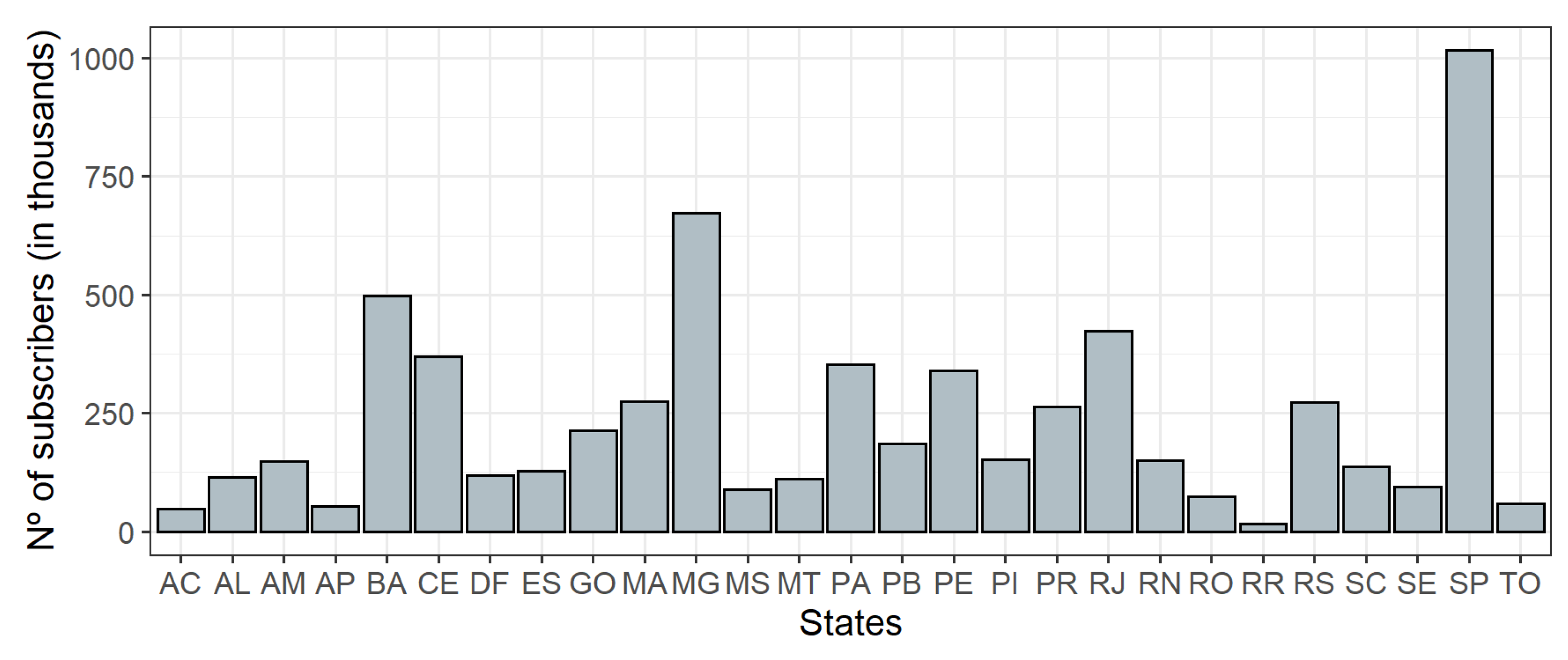
In order to understand the candidates situation in Brazil and learn more about the considered features, we carry out an Exploratory Data Analysis (EDA) to describe the profile of the 5,095,270 students who participated in ENEM 2019. Figure 5 shows the number of candidates across the 27 Brazilian Federative Units. In this plot, we can observe a large concentration of candidates in the states with a higher population density (São Paulo, Rio de Janeiro, Minas Gerais, Bahia, and Ceará States) and a smaller number of candidates in the states with the lowest population density (Roraima, Amapá, Acre, and Tocantins States).
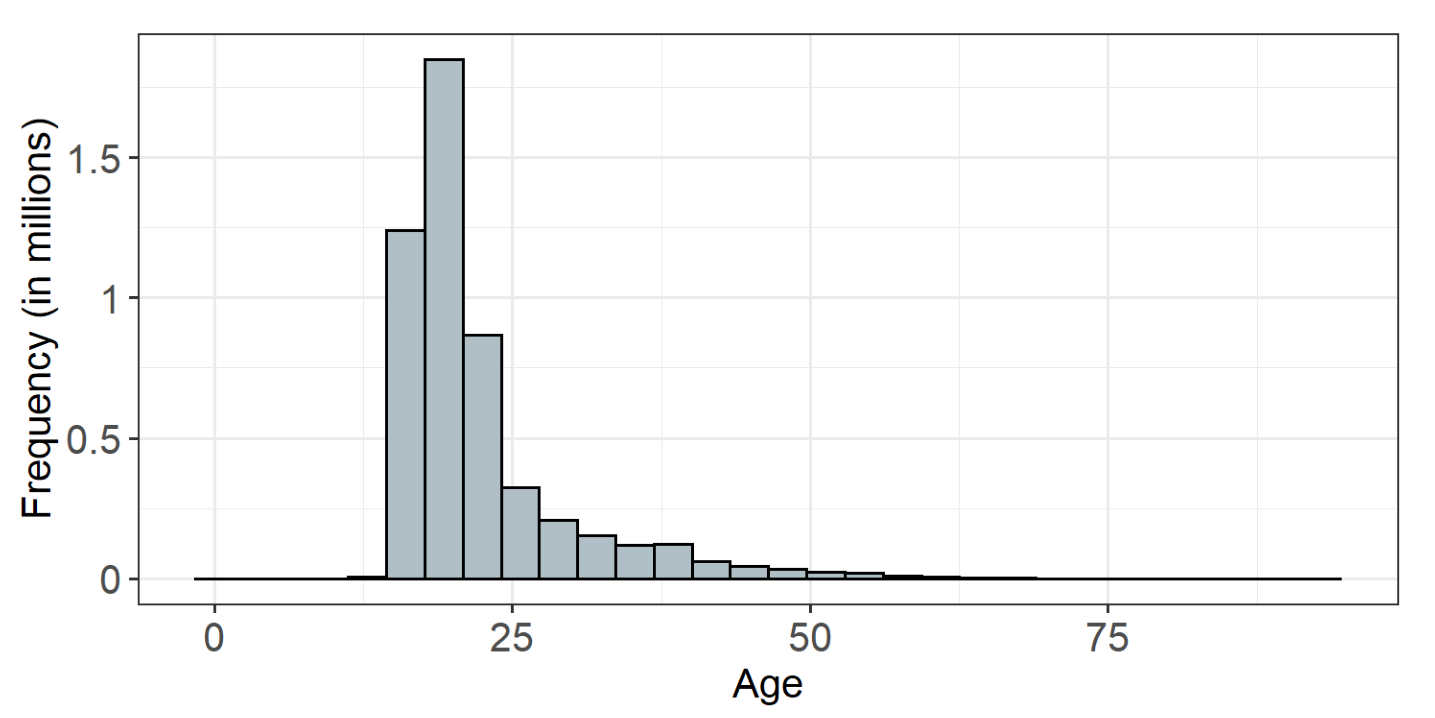
Figure 6 shows a histogram representing the distribution of students’ age. The asymmetrical shape is expected because many younger people usually register for the ENEM. The average age of 22 years is commonly observed because participants are typically students at the end of high school or those who have recently graduated, which can be confirmed by observing Table 3, which shows the large concentration of students who had completed high school or had completed it in 2019, the year that this exam was taken.
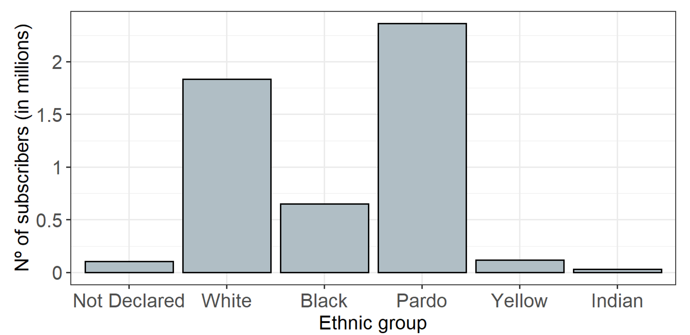
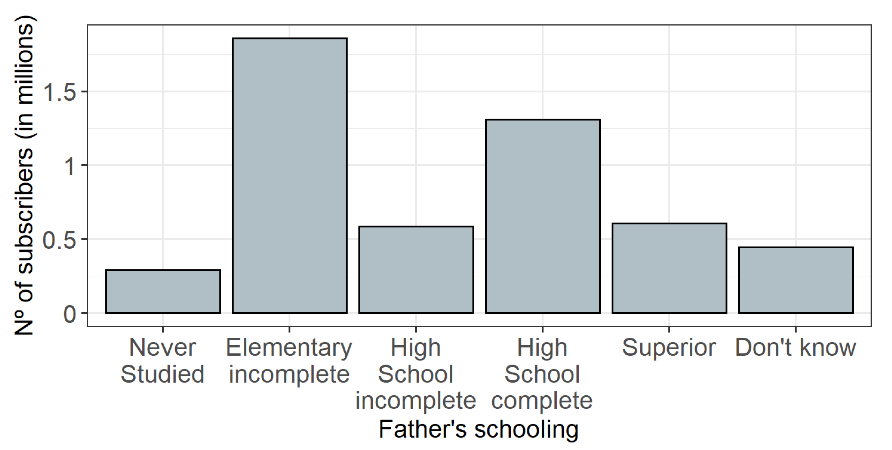
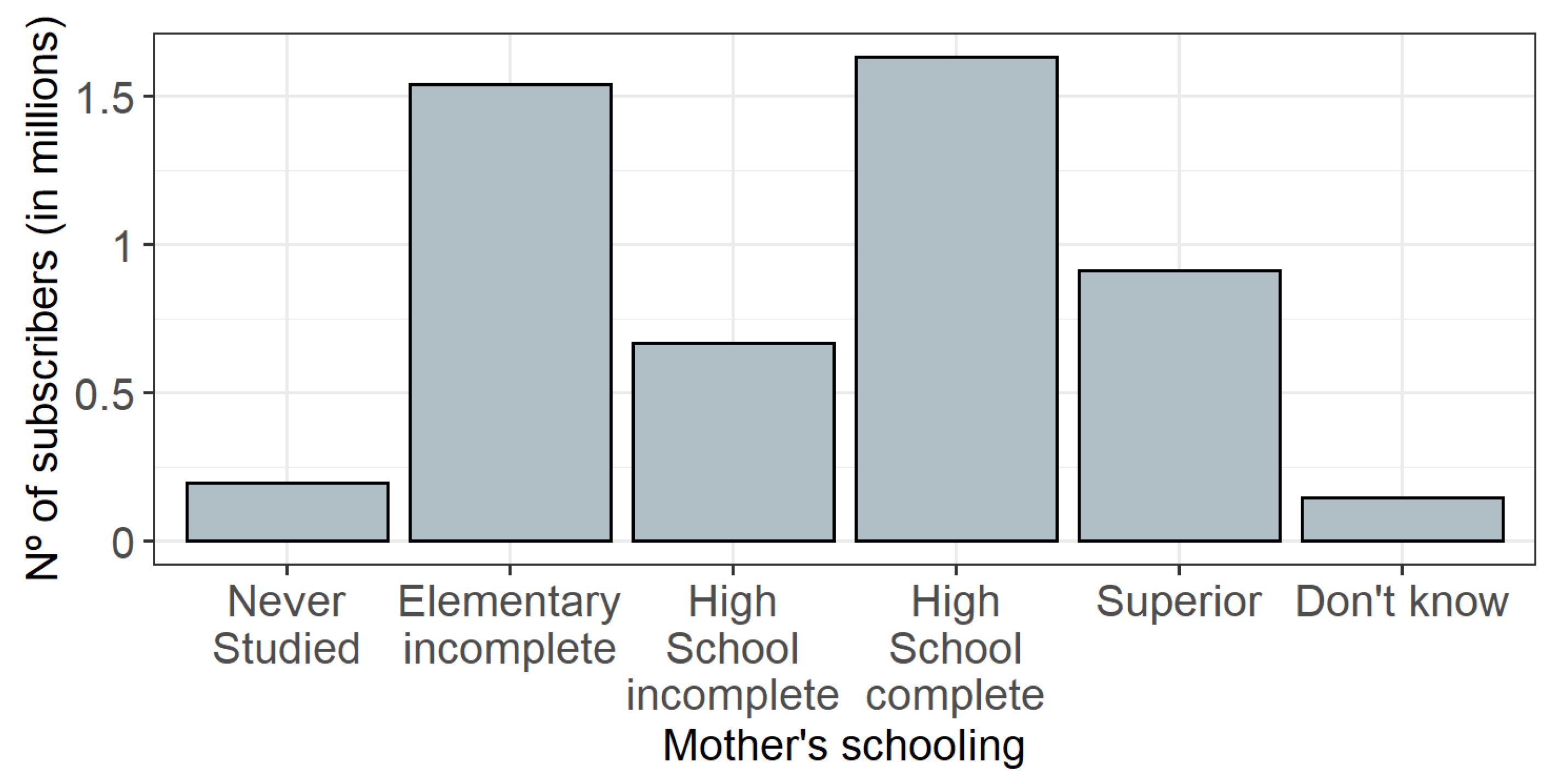
It can be seen that the largest number of candidates are female (3 million versus 2 million males). These values differ slightly comparatively from the Brazilian density population by gender [49]. On the other hand, around 600,000 students are identified as so-called trainee students (ENEM trainers are students under the age of 18 who are in their 1st or 2nd year of high school and wish to take the ENEM exam to test their knowledge). Figure 7 reveals the differences among candidates from different ethnic groups, with a concentration of applicants who declared themselves as Brown race (Pardo in Portuguese; Brown race is an official category used by the Brazilian Institute of Geography and Statistics-IBGE in the Brazilian census [50]). Figure 8 and Figure 9 show the most common level of education for fathers and mothers, where it was observed that mothers have a higher level of education when compared to fathers.
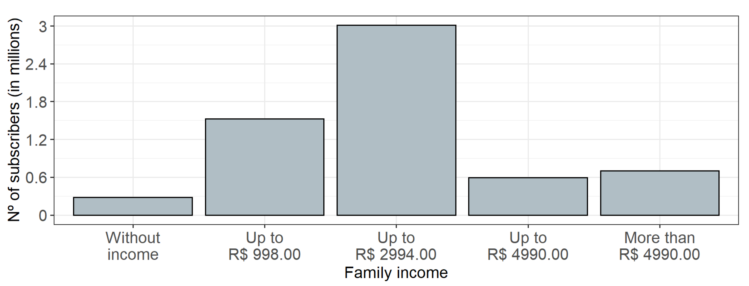
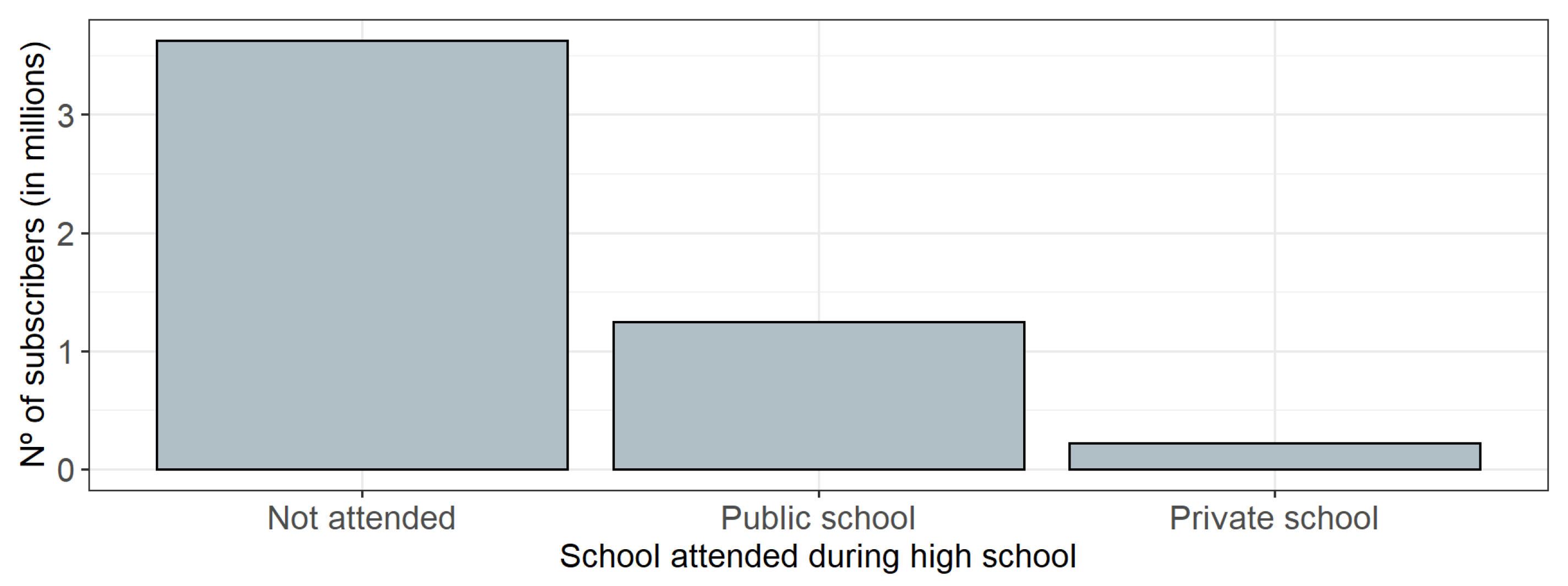
Figure 10 reveals a greater concentration of members with an income in the range of R $ 998.00 R $ 2 994.00 , followed by those with an income of up to R $ 998.00 . In addition to the personal information of these candidates, some characteristics related to their school life were analyzed. Thus, it was possible to observe that among the students who provided their year of completion of high school, 2018 was the year that registered the highest number of student candidates (600,000 candidates). In addition, we observed that in relation to the type of school attended during high school (See Figure 11), the vast majority of students chose not to provide this information; however, among those who did, it can be observed that most students had attended public schools.
By analyzing the choice of the language tests, we can observe in Table 4 a small difference between the number of registrants who chose English as a foreign language and the number of registrants who chose Spanish as a foreign language. Moreover, the data reveal an average rate of missing the tests of approximately 25%; less than 1% of the students were eliminated, typically candidates who violated an exam rule, and the test was removed in any of the four tests (see Table 5).
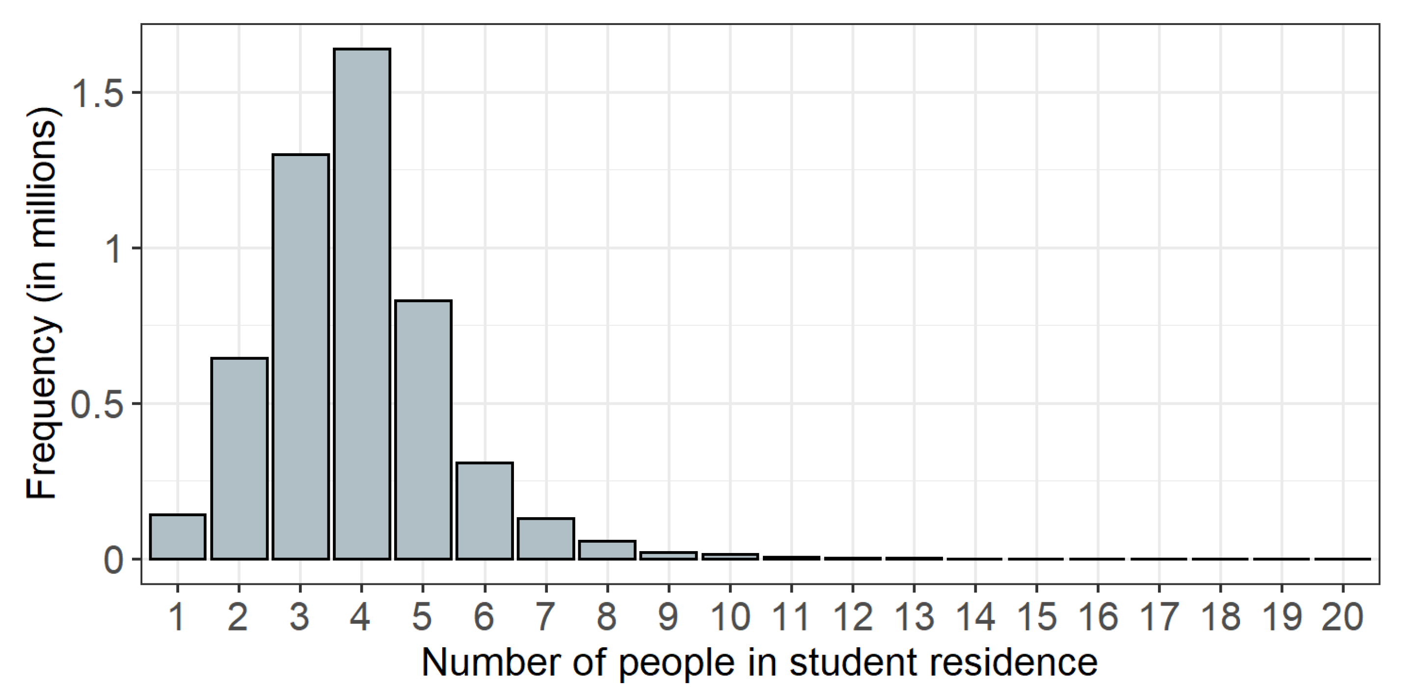
Observing the variable that shows the number of people who lived with the person enrolled in the ENEM (See Figure 12), it is noted that the vast majority of students shared a house with up to five people; this is an expected result given that, as this is an exam carried out mostly by students, they are expected to live with their families. In addition, there was also a high concentration of single candidates (86%), which once again is expected because participants were mostly young people at the end of school age.

5. Applications and Results

5.1. Modeling

This section presents the results obtained by modeling the average grades of students who took the ENEM 2019 using the variables listed in Table 2 as inputs of an SVR model. The results presented here correspond to the comparison between the so-called traditional SVR model, a model applied to all available data, and the model proposed in this paper, a model that applied pre-processing to extract the most informative observations that could thus reduce the time estimation needed for the final model and still maintain good predictive performance results. All analyses were performed using the 𝖱 [51] language on a personal computer with processor 2.00 GHz Intel Core i3-6006U, 4 GB RAM of memory, and a 64 bit Windows 10 Operating System. The 𝖱 codes are available from the authors upon request.
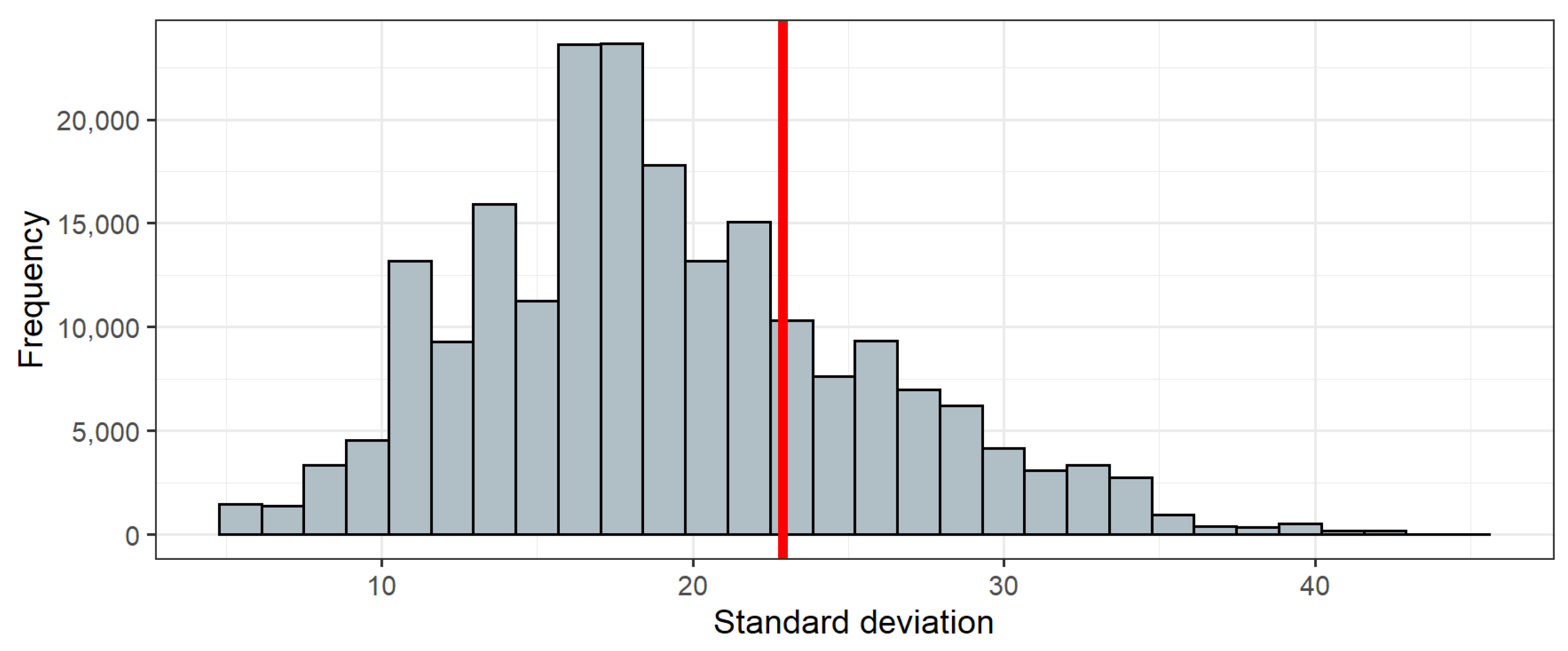
In order to use the proposed model, a total of K = 10 “Weak SVR” models were considered during the process, each constructed with n 0 = 1000 observations from the original training sample selected at random. In the observation selection process for the final training sample, the distribution of the calculated deviations for each observation can be seen in Figure 13. Thus, as previously defined, observations with a standard deviation greater than the value of the third quartile were selected as the final training sample. For the case of Figure 13, Q 3 = 22.90.
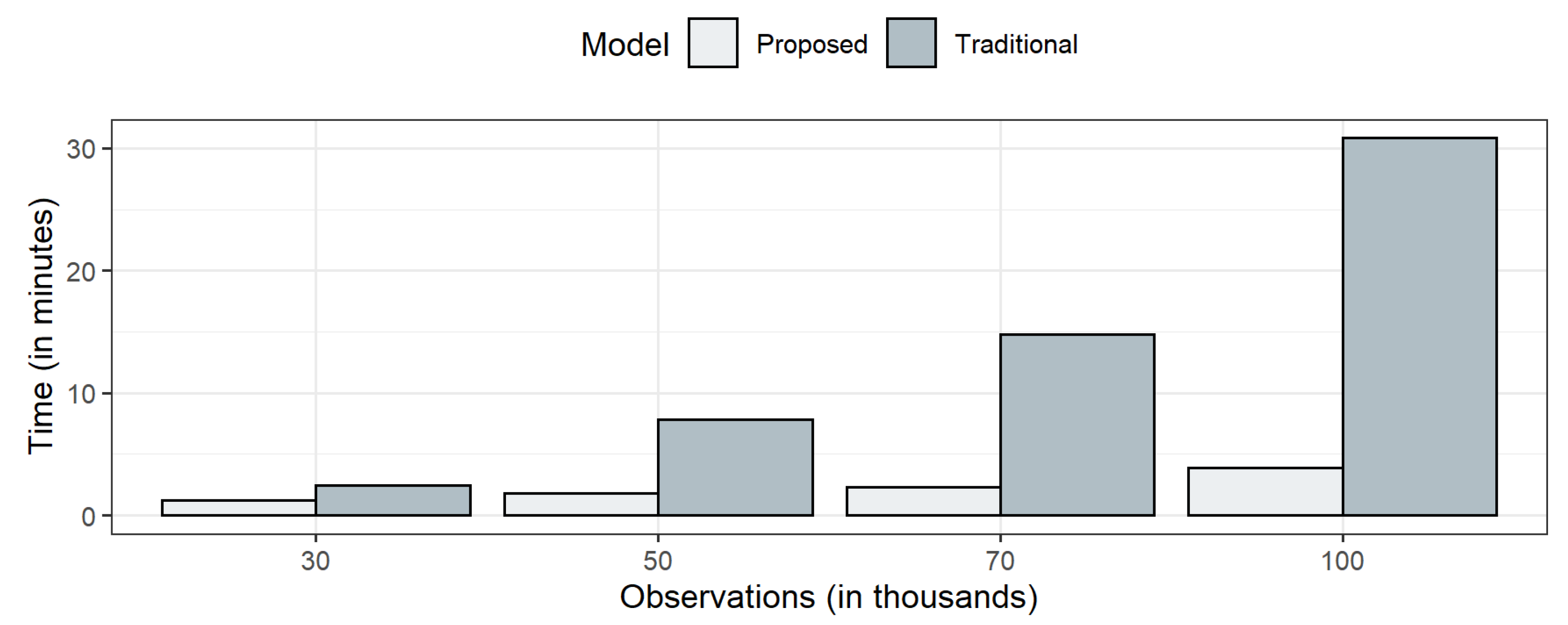
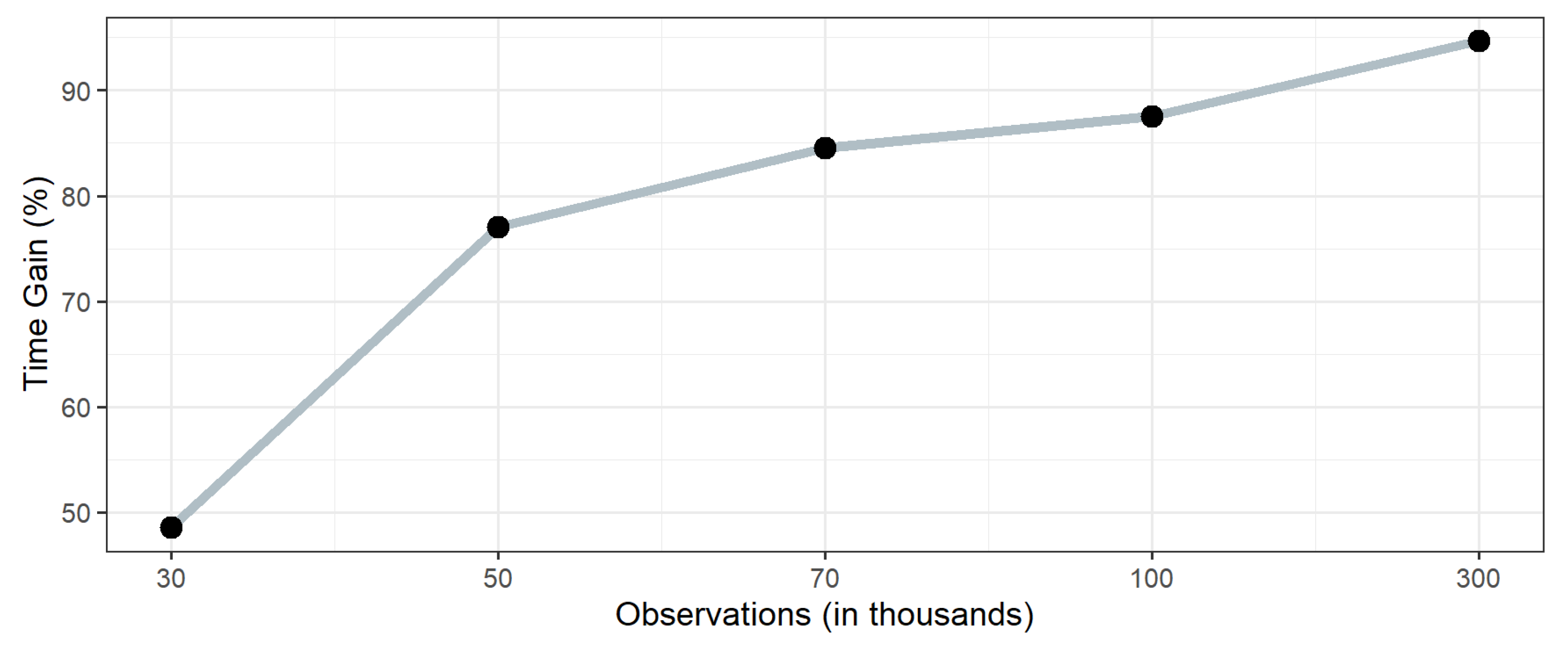
The evaluation of the proposed method considers different population sizes and the results are shown in Table 6, which considers 70% of observations as the training sample, as well as the Root Mean Squared Error (RMSE), Mean Absolute Error (MAE), and Mean Absolute Percentage Error (MAPE), as predictive performance measures in the test sample. Based on Figure 14, it is possible to observe the difference in time between the proposed model and the traditional SVR model, which includes all the observations in the estimation process. In addition, based on Table 6, it is observed that the quality of the adjustment was maintained, despite the small observed difference. Figure 15 shows the percentage gain in time performance when using the proposed model. It is possible to observe that the gain in time has a tendency of growth when also increasing the size of the base used, reaching a gain of 90% when working with a set with 300,000 observations, the largest set used in this comparison. Moreover, despite the use of a lower sample size, the obtained results of the proposed method are consistent with the traditional method for all the cases from 30,000 to 300,000 total observations. Furthermore, there was a reduction in the time needed for the learning phase, making it possible to observe the quality of the proposed model compared to the traditional model. In particular, the RMSE mostly presented values close to 70, which may be justified by the scale of the response variable, which varied between 0 and 900 points.
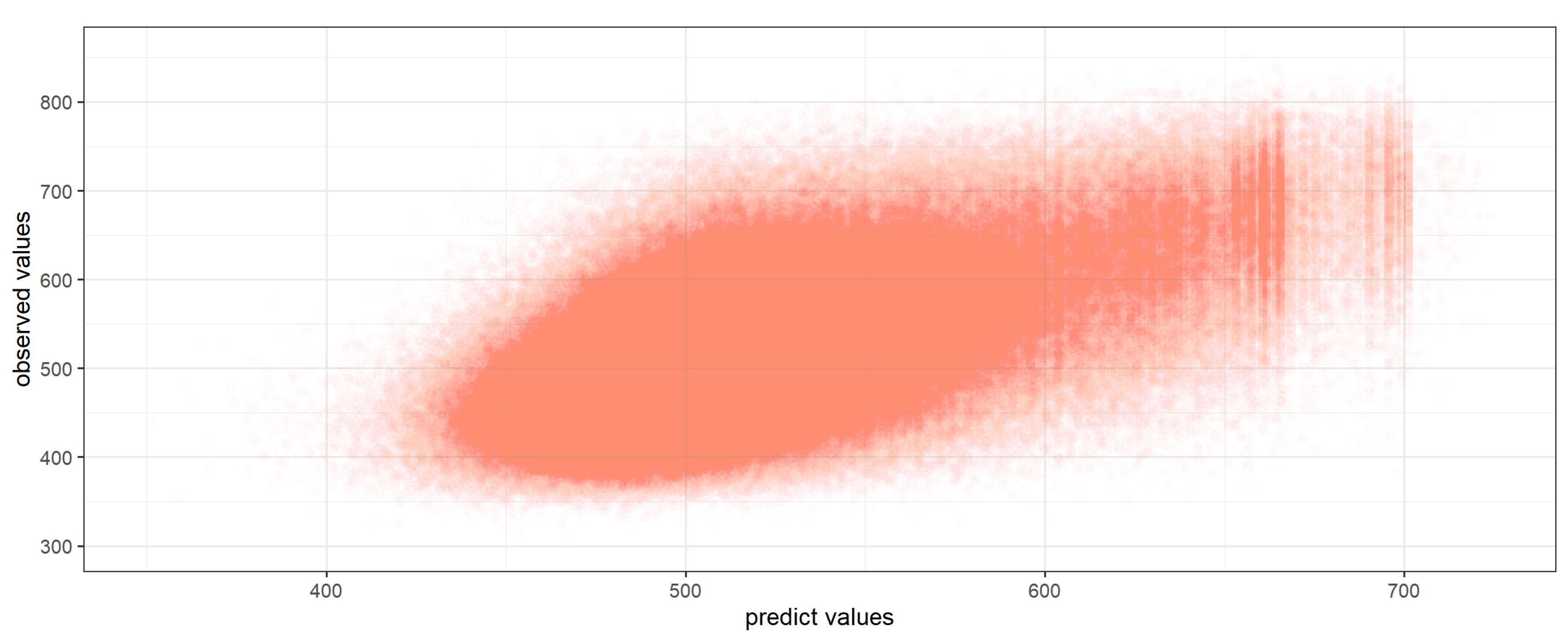
Furthermore, the general quality of the model’s fit was verified through the R 2 metric. As expected, it was 34%, which would indicate that the model is able to explain only 34% of the data variability. This value is consistent and close to other results found in the recent literature when performing a similar analysis using the ENEM database [52]. In particular, the metric R 2 is not the best metric to analyze the goodness of fit of a model, especially for a massive database such as ENEM, which presents great variability for its variable response. Figure 16 displays the behavior of the model when crossing the real values with the values predicted. Despite a behavior with high variability, as expected, it is possible to notice a moderate linear trend. It was also observed how the model behaved for each of the Brazilian geographic regions, thus taking the cross between the real and predicted values per region (see Figure 17). As seen for the whole country, there is a great variability in the predicted values; however, higher concentrations of notes are seen in the southeast and northeast regions of the country.

5.2. Comparative Analysis of the Predicted Grades

This section presents a comparative analysis performed between the worst and best predicted grades on the database, taking the top 10% and the bottom 10%; such analysis can be seen in Table 7. There is a significant difference between the behavior of some key variables used in the modeling, when comparing the worst grades with the best grades. The variable Ethnic group shows the great racial inequality existing in the country, while, among the worst average grades observed, there is a high concentration of self-declared brown students (62%); among the best average grades is seen a large concentration of students who were white (71%), and it is possible to observe a decline in the number of black students among those with better grades, a reduction from 20% to only 3%. Another important variable to be observed is the family income variable, which, in turn, shows economic inequality. While, among the worst grades, it is possible to observe a concentration of students with an income of 1 basic salary (R$ 998.00) (53%) and income between 1 basic salary and 3 basic salary (R$ 2994.00) (26%), for the best grades, there is an even greater concentration of students with a family income above 5 basic salary (R$ 4990.00) (72%), with less than 1% among the worst grades. Finally, two other important variables are the educational levels of the students’ parents. Among the worst grades, it is observed that the most common level of education is incomplete primary education, either for the father (49%) or for the mother (49%). On the other hand, for students who obtained the highest grades, there is a high number of mothers (71%) and fathers (62%) who completed higher education.

6. Final Considerations

Several high-profile publications have demonstrated a lack of transparency, reproducibility, ethics, and effectiveness in the reporting and evaluation of ML/AI-based predictive models (error rates) [53,54,55]. This growing body of evidence suggests that while many best practice recommendations for the design, performance, analysis, reporting, evaluation of student performance, and implementation of education and public policy can be borrowed from the traditional economics, public policy, health systems, and education statistics literature, they are not sufficient to guide the use of ML/IA in research. Producing such guidance with transparency and with intuitive methods is an important undertaking because of the increasing speed of producing predictions, the large battery of ML/IA algorithms, and the multifaceted nature of assessing student performance and social impact [56]. Taking no action is unacceptable, and if we wait for a more definitive solution, we risk breaking ethical and moral norms beyond the work of methodological development.
In particular, this paper presents some theoretical concepts about the SVR machine learning method, as well as a proposition to address the problem found when using this native regression method in large databases. The results obtained in the modeling process with the proposed model were traced as well as applied in an educational data mining problem. The proposed method maintained good performance and presented a considerable reduction in learning time, reaching a gain of 90% for a database with at least 300,000 observations. It represents a reduction in the time needed to learn the model from 8 h to only 26 min. This reduction was achieved only using theoretical modifications, without any use of parallel procedures.
The educational application provides a general descriptive analysis about the candidates who participated in the ENEM 2019 in Brazil, the distribution of the candidates by federative units, the economic situation of their families, the educational level of their parents, and also the distribution of high school type.
The learning time reduction and computational effort are quite relevant for online applications, since the learning step may be repeated in different subsets in dashboard applications, for example. In this sense, using only these seven input variables, it is possible to predict precisely the average grade of a student on the National High School Exam (ENEM—Exame Nacional do Ensino Médio) in Brazil. These efforts would be impractical when using SVR without a learning time reduction.
Based on the predictive results of the SVR, it is possible to determine the performance of a given student in a future ENEM test application: this can be key, on the one hand, to produce more comprehensive and fairer tests that account for the different demographics of students from different segments of society, i.e., the predictions allow the profiling of students and the grouping of them for various purposes, which mainly allows a reduction in inequality. On the other hand, the information assimilated by the algorithm can help us to understand more accurately the students’ learning processes and their interconnections in such a way that distortions can be corrected more quickly in teaching procedures.
Based on the experiment, we also found research limitations in our current study and identified more research methods for our future studies as follows. We observed that the number of students in the data set is an important factor affecting the predictive performance. For those subsets identified by region or ethnic group, for example, a larger number of students has better predictive performance; for example 10% better grades were found in a larger number of students with 60% ethnic group EG2 (high concentration). Nonetheless, predictions can be unstable if there is substantial volatility in the underlying data set or if the data set is small. Thus, in future work, it is necessary to introduce noise to improve the shortage of sample data. On the other hand, we observed that the method used in predicting students’ performance is based on a shallow architecture and predictive result failure to capture the relationships among attributes in a massive data set, and a similar conclusion was already presented [57,58] and others in similar works. It is also worth mentioning the fact that the work developed is easily extendable for other contexts and methods, and there is also the possibility for parallelization adequacy, which guarantees an even greater computational time gain, or even a combination within other methodologies applied in large databases [37,41].

Author Contributions

Conceptualization, A.A. and R.O.; methodology, A.A. and R.O.; software, J.S.P. and A.A.; validation, A.A. and J.S.P.; investigation, J.S.P., R.O. and A.A.; data curation, J.S.P.; writing—original draft preparation, J.S.P. and A.A.; writing—review and editing, R.O. and A.A.; supervision, A.A. All authors have read and agreed to the published version of the manuscript.

Funding

This work was partially supported by the National Council for Scientific and Technological Development (CNPq) through the grant 305305/2019-0 (R.O.) and Comissão de Aperfeiçoamento de Pessoal do Nível Superior (CAPES) number 001 in Brazil. The authors thank the editor and anonymous referees for comments and suggestions.

Institutional Review Board Statement

Not applicable.

Informed Consent Statement

Not applicable.

Conflicts of Interest

The authors declare no conflict of interest.

References

  1. Jaccoud, L.D.B.; Beghin, N. Desigualdades Raciais no Brasil: Um Balanço da Intervenção Governamental. Technical Report IPEA, 2002. Available online: http://repositorio.ipea.gov.br/handle/11058/9164 (accessed on 25 April 2020).
  2. Walker, J.; Pearce, C.; Boe, K.; Lawson, M. The Power of Education to Fight Inequality: How Increasing Educational Equality and Quality Is Crucial to Fighting Economic and Gender Inequality. 2019. Available online: https://oxfamilibrary.openrepository.com/handle/10546/620863 (accessed on 1 July 2021).
  3. Hamel, L.H. Knowledge Discovery with Support Vector Machines; John Wiley & Sons, Inc.: Hoboken, NJ, USA, 2011; Volume 3. [Google Scholar]
  4. Cortes, C.; Vapnik, V. Support-vector networks. Mach. Learn. 1995, 20, 273–297. [Google Scholar] [CrossRef]
  5. Shivaswamy, P.K.; Chu, W.; Jansche, M. A support vector approach to censored targets. In Proceedings of the Seventh IEEE International Conference on Data Mining (ICDM 2007), Omaha, NE, USA, 28–31 October 2007; pp. 655–660. [Google Scholar]
  6. Liang, J.; Yang, J.; Wu, Y.; Li, C.; Zheng, L. Big data application in education: Dropout prediction in edx MOOCs. In Proceedings of the 2016 IEEE Second International Conference on Multimedia Big Data (BigMM), Taipei, Taiwan, 20–22 April 2016; pp. 440–443. [Google Scholar]
  7. Mite-Baidal, K.; Delgado-Vera, C.; Solís-Avilés, E.; Espinoza, A.H.; Ortiz-Zambrano, J.; Varela-Tapia, E. Sentiment analysis in education domain: A systematic literature review. In International Conference on Technologies and Innovation; Springer: Cham, Switzerland, 2018; pp. 285–297. [Google Scholar]
  8. Pujianto, U.; Zaeni, I.A.E.; Irawan, N.O. SVM Method for Classification of Primary School Teacher Education Journal Articles. In Proceedings of the 2019 International Conference on Electrical, Electronics and Information Engineering (ICEEIE), Denpasar, Indonesia, 3–4 October 2019; Volume 6, pp. 324–329. [Google Scholar]
  9. Ranjeeth, S.; Latchoumi, T.; Sivaram, M.; Jayanthiladevi, A.; Kumar, T.S. Predicting Student Performance with ANNQ3H: A Case Study in Secondary Education. In Proceedings of the 2019 International Conference on Computational Intelligence and Knowledge Economy (ICCIKE), Dubai, United Arab Emirates, 11–12 December 2019; pp. 603–607. [Google Scholar]
  10. López-Martín, C.; Ulloa-Cazarez, R.L.; García-Floriano, A. Support vector regression for predicting the productivity of higher education graduate students from individually developed software projects. IET Softw. 2017, 11, 265–270. [Google Scholar] [CrossRef]
  11. Fefilatyev, S.; Smarodzinava, V.; Hall, L.O.; Goldgof, D.B. Horizon detection using machine learning techniques. In Proceedings of the 2006 5th International Conference on Machine Learning and Applications (ICMLA’06), Orlando, FL, USA, 14–16 December 2006; pp. 17–21. [Google Scholar]
  12. Ahmad, I.; Basheri, M.; Iqbal, M.J.; Rahim, A. Performance comparison of support vector machine, random forest, and extreme learning machine for intrusion detection. IEEE Access 2018, 6, 33789–33795. [Google Scholar] [CrossRef]
  13. Libbrecht, M.W.; Noble, W.S. Machine learning applications in genetics and genomics. Nat. Rev. Genet. 2015, 16, 321–332. [Google Scholar] [CrossRef] [Green Version]
  14. Shi, P.; Ray, S.; Zhu, Q.; Kon, M.A. Top scoring pairs for feature selection in machine learning and applications to cancer outcome prediction. BMC Bioinform. 2011, 12, 1–15. [Google Scholar] [CrossRef] [Green Version]
  15. Huang, S.; Cai, N.; Pacheco, P.P.; Narrandes, S.; Wang, Y.; Xu, W. Applications of support vector machine (SVM) learning in cancer genomics. Cancer Genom. Proteom. 2018, 15, 41–51. [Google Scholar]
  16. Bartlett, M.S.; Littlewort, G.; Frank, M.; Lainscsek, C.; Fasel, I.; Movellan, J. Recognizing facial expression: Machine learning and application to spontaneous behavior. In Proceedings of the 2005 IEEE Computer Society Conference on Computer Vision and Pattern Recognition (CVPR’05), San Diego, CA, USA, 20–25 June 2005; Volume 2, pp. 568–573. [Google Scholar]
  17. Zendehboudi, A.; Baseer, M.; Saidur, R. Application of support vector machine models for forecasting solar and wind energy resources: A review. J. Clean. Prod. 2018, 199, 272–285. [Google Scholar] [CrossRef]
  18. Amorim, M.J.; Barone, D.; Mansur, A.U. Técnicas de Aprendizado de Máquina Aplicadas na Previsao de Evasão Acadêmica. In Brazilian Symposium on Computers in Education (Simpósio Brasileiro de Informática na Educação-SBIE); 2008; Volume 1, pp. 666–674. Available online: https://www.semanticscholar.org/paper/T%C3%A9cnicas-de-Aprendizado-de-M%C3%A1quina-Aplicadas-na-de-Amorim-Barone/7b547c1ccb2b24cc16e5da6dcf2ea0922bb32bf9 (accessed on 1 July 2021).
  19. Romero, C.; Ventura, S. Educational data mining and learning analytics: An updated survey. Wiley Interdiscip. Rev. 2020, 10, e1355. [Google Scholar] [CrossRef]
  20. Campbell, C.; Levin, B. Using data to support educational improvement. Educ. Assess. Eval. Account. 2009, 21, 47. [Google Scholar] [CrossRef]
  21. Chiquetto, M.J.; Krapas, S. Livros didáticos baseados em apostilas: Como surgiram e por que foram amplamente adotados. Revista Brasileira de Pesquisa em Educação em Ciências 2012, 12, 173–191. [Google Scholar]
  22. Motz, B.A.; Carvalho, P.F.; de Leeuw, J.R.; Goldstone, R.L. Embedding experiments: Staking causal inference in authentic educational contexts. J. Learn. Anal. 2018, 5, 47–59. [Google Scholar] [CrossRef] [Green Version]
  23. Wu, P.; Dietterich, T.G. Improving SVM accuracy by training on auxiliary data sources. In Proceedings of the Twenty-First International Conference on Machine Learning, Banff, AB, Canada, 4–8 July 2004; p. 110. [Google Scholar]
  24. Huang, J.; Saleh, S.; Liu, Y. A Review on Artificial Intelligence in Education. Acad. J. Interdiscip. Stud. 2021, 10, 206. [Google Scholar] [CrossRef]
  25. Mahareek, E.A.; Desuky, A.S.; El-Zhni, H.A. Simulated annealing for SVM parameters optimization in student’s performance prediction. Bull. Electr. Eng. Inform. 2021, 10, 1211–1219. [Google Scholar] [CrossRef]
  26. Wang, S.; Li, Z.; Liu, C.; Zhang, X.; Zhang, H. Training data reduction to speed up SVM training. Appl. Intell. 2014, 41, 405–420. [Google Scholar] [CrossRef]
  27. Campbell, C.; Ying, Y. Learning with support vector machines. Synth. Lect. Artif. Intell. Mach. Learn. 2011, 5, 1–95. [Google Scholar] [CrossRef]
  28. Boser, B.E.; Guyon, I.M.; Vapnik, V.N. A training algorithm for optimal margin classifiers. In Proceedings of the Fifth Annual Workshop on Computational Learning Theory, Pittsburgh, PA, USA, 27–29 July, 1992; pp. 144–152. [Google Scholar]
  29. Vapnik, V.N. The Nature of Statistical Learning Theory; Springer: New York, NY, NY, 1995. [Google Scholar]
  30. Vapnik, V.N. Statistical Learning Theory; Wiley-Interscience: Hoboken, NJ, USA, 1998. [Google Scholar]
  31. Batalha, C. Modelos de Vetores de Suporte em séries Temporais: Uma Aplicaçãopara Criptomoedas. Master’s Thesis, Universidade Federal da Bahia, Salvador, Bahia, Brasil, 2019. [Google Scholar]
  32. Smola, A.J.; Schölkopf, B. A tutorial on support vector regression. Stat. Comput. 2004, 14, 199–222. [Google Scholar] [CrossRef] [Green Version]
  33. Yaohao, P. Support Vector Regression Aplicado à Previsão de taxas de Câmbio. 2016. Available online: https://repositorio.unb.br/bitstream/10482/23270/1/2016_PengYaohao.pdf (accessed on 15 October 2020).
  34. Lin, P.T.; Su, S.F.; Lee, T.T. Support vector regression performance analysis and systematic parameter selection. In Proceedings of the 2005 IEEE International Joint Conference on Neural Networks, Montreal, QC, Canada, 31 July–4 August 2005; Volume 2, pp. 877–882. [Google Scholar]
  35. Platt, J. Sequential Minimal Optimization: A Fast Algorithm for Training Support Vector Machines; Technical Report MSR-TR-98-14; Microsoft Research: 1998. Available online: https://www.microsoft.com/en-us/research/publication/sequential-minimal-optimization-a-fast-algorithm-for-training-support-vector-machines/ (accessed on 1 July 2021).
  36. Fan, R.E.; Chen, P.H.; Lin, C.J.; Joachims, T. Working set selection using second order information for training support vector machines. J. Mach. Learn. Res. 2005, 6, 889–1918. [Google Scholar]
  37. Tsang, I.W.; Kwok, J.T.; Cheung, P.M.; Cristianini, N. Core vector machines: Fast SVM training on very large data sets. J. Mach. Learn. Res. 2005, 6, 363–392. [Google Scholar]
  38. Sarmento, P.L. Avaliação de Métodos de Seleção de Amostras Para redução do Tempo de Treinamento do Classificador SVM. Master’s Thesis, INPE, Sao Jose dos Campos, São Paulo, Brazil, 2014. [Google Scholar]
  39. Lee, Y. Handwritten digit recognition using k nearest-neighbor, radial-basis function, and backpropagation neural networks. Neural Comput. 1991, 3, 440–449. [Google Scholar] [CrossRef] [PubMed]
  40. Lawrence, S.; Giles, C.L.; Tsoi, A.C.; Back, A.D. Face recognition: A convolutional neural-network approach. IEEE Trans. Neural Networks 1997, 8, 98–113. [Google Scholar] [CrossRef] [Green Version]
  41. Torres-Barrán, A.; Alaíz, C.M.; Dorronsoro, J.R. Faster SVM training via conjugate SMO. Pattern Recognit. 2021, 111, 107644. [Google Scholar] [CrossRef]
  42. Shalev-Shwartz, S.; Srebro, N. SVM optimization: Inverse dependence on training set size. In Proceedings of the 25th International Conference on Machine Learning, New York, NY, USA, 5–9 July, 2008; pp. 928–935. [Google Scholar]
  43. Shalev-Shwartz, S.; Singer, Y.; Srebro, N.; Cotter, A. Pegasos: Primal estimated sub-gradient solver for svm. Math. Program. 2011, 127, 3–30. [Google Scholar] [CrossRef] [Green Version]
  44. Fan, R.E.; Chang, K.W.; Hsieh, C.J.; Wang, X.R.; Lin, C.J. LIBLINEAR: A library for large linear classification. J. Mach. Learn. Res. 2008, 9, 1871–1874. [Google Scholar]
  45. Lee, Y.J.; Mangasarian, O.L. RSVM: Reduced support vector machines. In Proceedings of the 2001 SIAM International Conference on Data Mining, SIAM, Chicago, IL, USA, 5–7 April 2001; pp. 1–17. [Google Scholar]
  46. Ebrey, P.B.; Ebrey, P.B.; Ebrey, P.B.; Ebrey, P.B. The Cambridge Illustrated History of China; Cambridge University Press: Cambridge, UK, 1996; Volume 1. [Google Scholar]
  47. Viggiano, E.; Mattos, C. O desempenho de estudantes no Enem 2010 em diferentes regiões brasileiras. Revista Brasileira de Estudos Pedagógicos 2013, 94, 417–438. [Google Scholar] [CrossRef] [Green Version]
  48. Bastos, C. Inscrições no Enem Crescem 20 Vezes Desde 1998. Portal do MEC. 2006. Available online: http://portal.mec.gov.br/ultimas-noticias/201-266094987/6881-sp-1649249425 (accessed on 10 May 2020).
  49. IBGE. Censo Brasileiro de 2010. Ibge-Instituto Brasileiro de Geografia e EstatíStica. Rio de Janeiro. 2012. Available online: https://censo2010.ibge.gov.br/ (accessed on 1 July 2021).
  50. IBGE. Technical Research: Pesquisa Nacional por Amostra de Domicílios. 2005. Available online: https://www.ibge.gov.br/estatisticas/sociais/populacao/9127-pesquisa-nacional-por-amostra-de-domicilios.html?=&t=o-que-e (accessed on 1 July 2021).
  51. R Core Team. R: A Language and Environment for Statistical Computing. 2013. Available online: r.meteo.uni.wroc.pl/web/packages/dplR/vignettes/intro-dplR.pdf (accessed on 1 July 2021).
  52. Stearns, B.; Rangel, F.M.; Rangel, F.; de Faria, F.F.; Oliveira, J.; Ramos, A.A.d.S. Scholar Performance Prediction Using Boosted Regression Trees Techniques; ESANN: Bruges, Belgium, 2017. [Google Scholar]
  53. Cortes, C.; Jackel, L.D.; Chiang, W.P. Limits on learning machine accuracy imposed by data quality. KDD 1995, 95, 57–62. [Google Scholar]
  54. Aziz, O.; Klenk, J.; Schwickert, L.; Chiari, L.; Becker, C.; Park, E.J.; Mori, G.; Robinovitch, S.N. Validation of accuracy of SVM-based fall detection system using real-world fall and non-fall datasets. PLoS ONE 2017, 12, e0180318. [Google Scholar] [CrossRef] [PubMed] [Green Version]
  55. Reiss, M. The use of AI in education: Practicalities and ethical considerations. Lond. Rev. Educ. 2021, 19, 1–14. [Google Scholar]
  56. Tuomi, I. The Impact of Artificial Intelligence on Learning, Teaching, and Education; Publications Office of the European Union: Luxembourg, 2018. [Google Scholar]
  57. Guo, B.; Zhang, R.; Xu, G.; Shi, C.; Yang, L. Predicting students performance in educational data mining. In Proceedings of the 2015 International Symposium on Educational Technology (ISET), Wuhan, China, 27–29 July 2015; pp. 125–128. [Google Scholar]
  58. Huang, A.Y.; Lu, O.H.; Huang, J.C.; Yin, C.; Yang, S.J. Predicting students’ academic performance by using educational big data and learning analytics: Evaluation of classification methods and learning logs. Interact. Learn. Environ. 2020, 28, 206–230. [Google Scholar] [CrossRef]
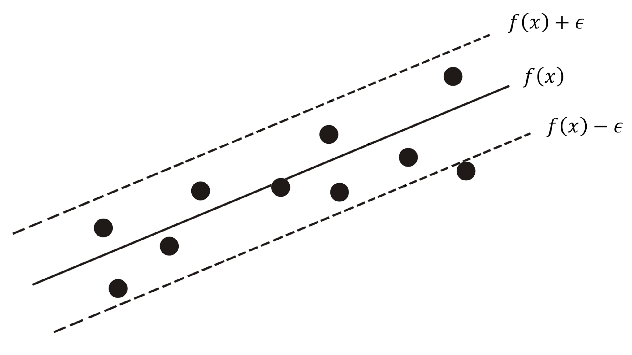
Figure 1. SVR representation. The black dots are the observations in raw representation. Adapted from [31].
Stats 04 00041 g001
Figure 2. SVR with slack variables. The black dots are the observations in raw representation. Adapted from [31].
Stats 04 00041 g002
Figure 3. Kernel trick. Adapted from [33].
Stats 04 00041 g003
Figure 4. Approach used to reduce the training time of the traditional SVR algorithm.
Stats 04 00041 g004
Figure 5. Distribution of the candidates by Brazilian Federative Unit.
Stats 04 00041 g005
Figure 6. Histogram of the age of the candidates.
Stats 04 00041 g006
Figure 7. Distribution of candidates by ethnic group.
Stats 04 00041 g007
Figure 8. Distribution of candidates according to father’s education.
Stats 04 00041 g008
Figure 9. Distribution of candidates according to mother’s education.
Stats 04 00041 g009
Figure 10. Distribution of candidates by family income.
Stats 04 00041 g010
Figure 11. Distribution of candidates by type of school attended in high school.
Stats 04 00041 g011
Figure 12. Number of people who shared residence with candidates.
Stats 04 00041 g012
Figure 13. Standard deviation distribution. The vertical line shows the quartile cut-off point used for selecting observations.
Stats 04 00041 g013
Figure 14. Adjustment times of traditional and proposed models.
Stats 04 00041 g014
Figure 15. Percentage of time gain between the traditional and proposed models.
Stats 04 00041 g015
Figure 16. Predicted values vs. real values.
Stats 04 00041 g016
Figure 17. Predicted values vs. real values by Brazilian geographic region.
Stats 04 00041 g017
Table 1. Most common kernels.
Kernel Type K ( x i , x j ) Parameters
Linear σ x , x j + d σ , d
Polynomial σ x i , x j + d q σ , d , q
Gaussian exp | | x i x j | | 2 2 σ 2 σ
Table 2. Subset of variables to be used.
DescriptionVariableScaleLabels
AgeNU_IDADENumeric10, …, 90
GenderTP_SEXOCategoricalM = Male, F = Female
Ethnic groupTP_COR_RACACategoricalNot Declared, White, Brown, Black, Yellow, Indigenous
Marital StatusTP_ESTADO_CIVILCategoricalNot Informed, Single, Married, Divorced, Widowed
Family incomeQ006CategoricalWithout Income, <998, 998–2994, 2994–4990, 4990+
High School Completion StatusTP_ST_CONCLUSAOCategoricalComplete High School, Completion in 2019, Incomplete High School
Conclusion yearTP_ANO_CONCLUIUCategoricalNot Informed, 2016–2018, <2016
High School TypeTP_ESCOLACategoricalPublic, Private, Not attended
Foreign LanguageTP_LINGUACategoricalEnglish, Spanish
Father’s EducationQ001CategoricalNever studied, Elementary incomplete, High school incomplete, High school complete, Superior, Don’t know
Mother’s EducationQ002CategoricalNever studied, Elementary incomplete, High school incomplete, High school complete, Superior, Don’t know
Number of people in student residenceQ005Numeric1, …, 20
Table 3. High school completion status.
Complete High SchoolCompletion in 2019Completion after 2019Incomplete High School
59%28%12%1%
Table 4. Distribution of candidates by foreign language.
EnglishSpanish
2.4 million2.6 million
Table 5. Situation of participants in objective tests and writing.
HumanitiesNature SciencesLanguagesMathematicsWriting
Absent22.9%27.1%22.9%27.1%23%
Present77%72.8%77%72.8%74.2%
Eliminated0.1%0.1%0.1%0.1%2.8%
Table 6. Evaluation of the proposed model for different population sizes.
SampleRMSEMAEMAPE (%)
30 k observations
Traditional Method21,00072.8357.2357.27
Proposed Method525074.6458.9357.58
50 k observations
Traditional Method35,00072.1856.4911.13
Proposed Method873272.7856.9611.18
70 k observations
Traditional Method49,00071.9456.6311.14
Proposed Method12,24972.7457.4311.31
100 k observations
Traditional Method70,00072.2256.7811.18
Proposed Method17,50072.6857.2811.27
300 k observations
Traditional Method210,00072.2356.7516.70
Proposed Method52,05573.4757.8317.13
Table 7. Comparative analysis between the best average grades and the worst average grades.
Variables10% Worse Grades10% Better Grades
Age: Average; SD; [Min, Max]26.74; 10.29; [13, 86]19.57; 4.29; [2, 68]
Gender: Male (%)/Female (%)24/7649/51
Ethnic group: EG1 (%)/EG2 (%)/EG3 (%)/EG4 (%)/EG5 (%)/EG6 (%)2/11/20/62/2.5/2.53/71/3/20/2.5/0.5
Marital Status: Not Informed (%)/Single (%)/Married (%)/Divorced (%)/Widowed (%)5/80/12/2/12.5/95/2/0.4/0.1
High School Type: Not attended (%)/Public (%)/Private (%)61/38/156/3/41
High School Completion Status: HSS1 (%)/HSS2 (%)/HSS3 (%)60/39/155/44/1
Conclusion year: Not Informed (%)/2016-2018 (%)/<2016 (%)45/26/2944/37/19
Foreign Language: English (%)/Spanish (%)16/8490/10
Father’s Education: FE1 (%)/FE2 (%)/FE3 (%)/FE4 (%)/FE5 (%)/FE6 (%)23/49/5/4.5/0.5/170.5/4/4.5/28/62/1
Mother’s Education: ME1 (%)/ME2 (%)/ME3 (%)/ME4 (%)/ME5 (%)/ME6 (%)19/49/9/10/1/120.1/1/2/25/71/0.9
Number of people in student residence: Average; SD; [Min, Max]4.5; 1.92; [1, 20]3.6; 1.06; [1, 11]
Family income: FI1 (%)/FI2 (%)/FI3 (%)/FI4 (%)/FI5 (%)20/53/26/0.5/0.50.5/0.5/7/20/72
Average Grade Predicted: Average; SD; [Min, Max]455.07; 13.15; [347.55, 469.85]643.14; 24.56; [606.85, 734.26]
EG1 = Not Declared, EG2 = White, EG3 = Brown, EG4 = Black, EG5 = Yellow, EG6 = Indigenous. HSS1 = Complete High School, HSS2 = Completionin 2019, HSS3 = Incomplete High School. FE1 and ME1 = Never studied, FE2 and ME2 = Elementary incomplete, FE3 and ME3 = High school incomplete, FE4 and ME4 = High school complete, FE5 and ME5 = Superior, FE6 and ME6 = Don’t know. FI1 = Without Income, FI2 = <998, FI3 = 998–2994, FI4 = 2994–4990, FI5 = 4990+.
Publisher’s Note: MDPI stays neutral with regard to jurisdictional claims in published maps and institutional affiliations.