Table of Contents
The First Digit on the Left Side of Numbers
Benford’s Law and the Predominance of Low Digits
Second Digits, Third Digits, and Higher Order Digits
A Robust Measure of Order of Magnitude (ROM)
Two Essential Requirements for Benford Behavior
Three Generic Causes of the Benford Phenomenon
The chi-square Test in the Context of Benford’s Law
The First Paradox
The Second Paradox
The Proper Use and Context of the chi-square Application
The Statistical Theory Forming the Basis for the Chi-Square Test
Comparison of the chi-square Statistic with SSD
Testing the Lognormal via the Chi-Square Statistic
Testing the Fibonacci Series via the Chi-Square Statistic
Testing Partial US Population Data Sets via the Chi-Square Statistic
The Nature of Hypothetical Real-Life-Like Revenue Data
The Nature of Hypothetical Real-Life-Like Population Data
Conclusions
1. The First Digit on the Left Side of Numbers
It has been discovered that the first digit on the left-most side of numbers in real-life data sets is most commonly of low value, such as {1, 2, 3}, and rarely of high value, such as {7, 8, 9}.
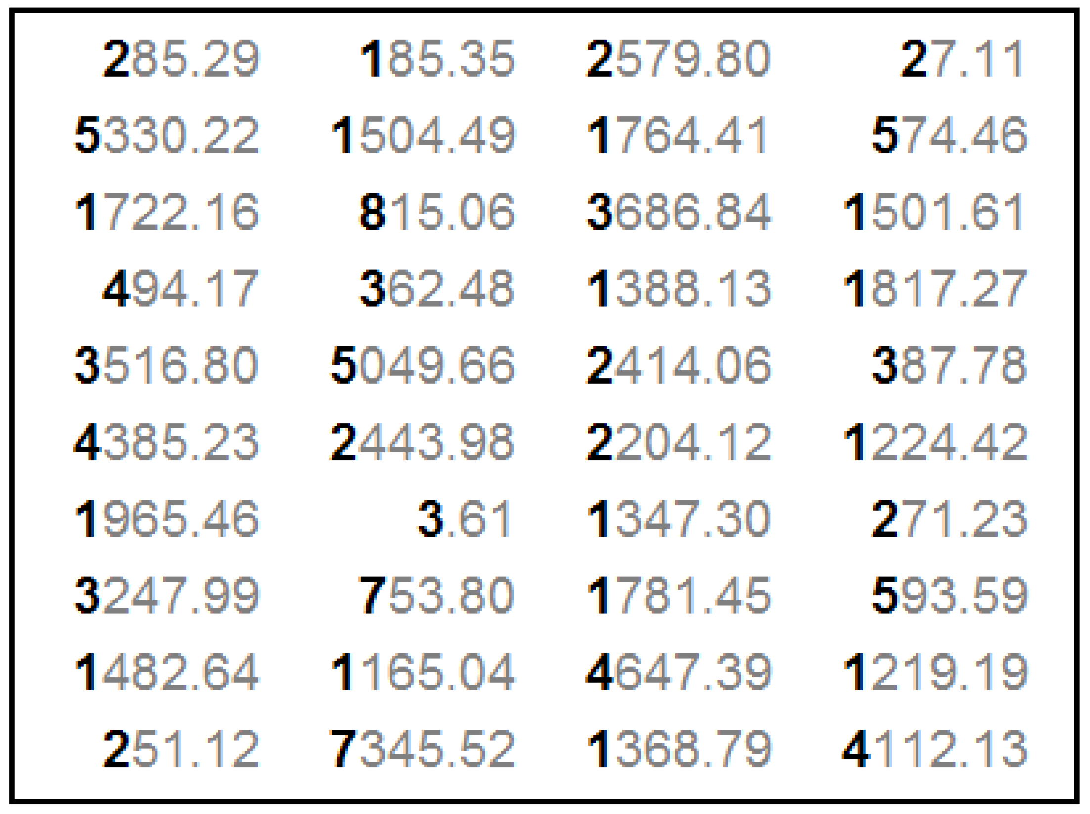
As an example serving as a brief and informal empirical test, a small sample of 40 values relating to geological data on time between successive earthquakes is randomly chosen from the data set on all global earthquake occurrences in 2012—in units of seconds.
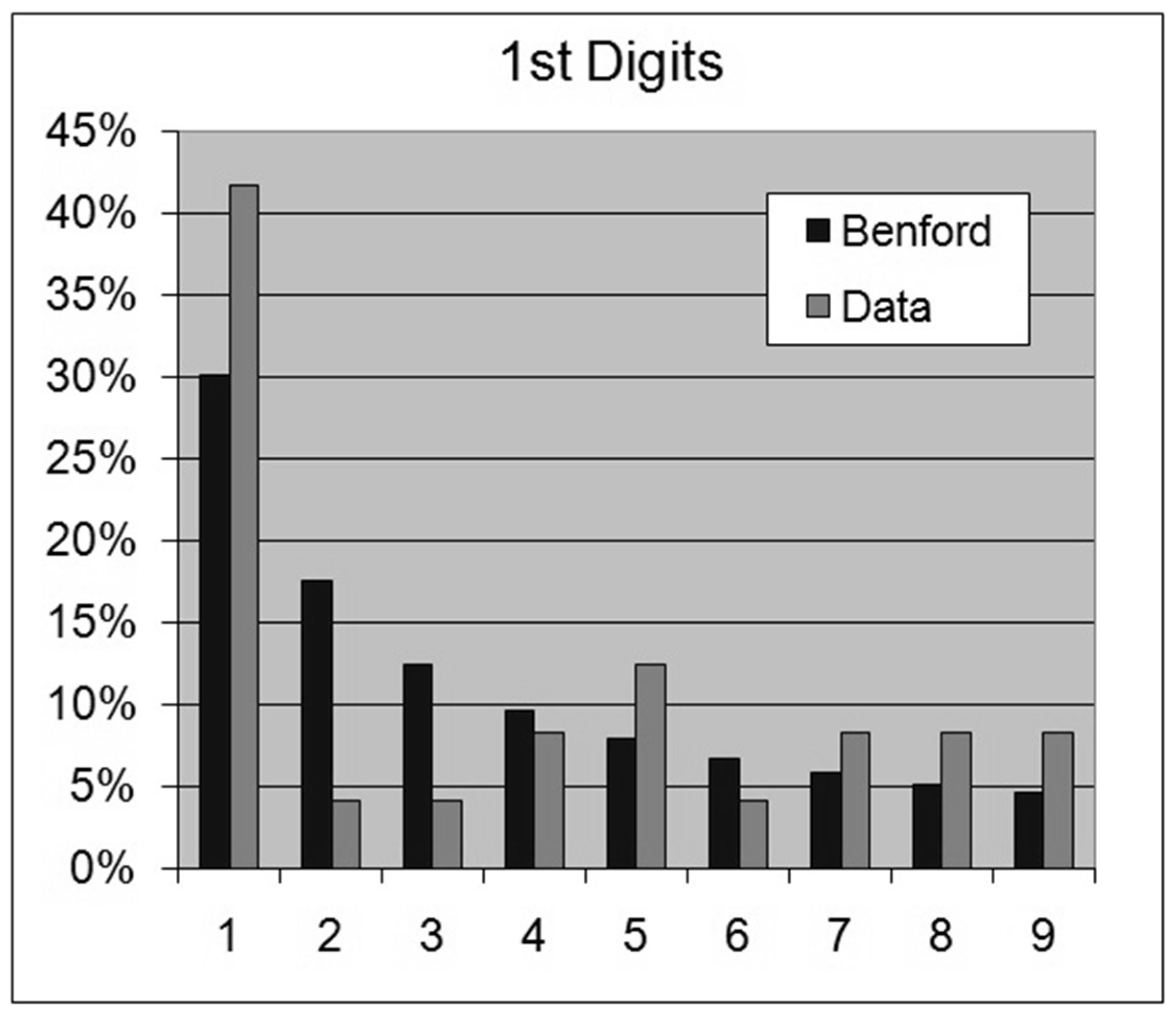
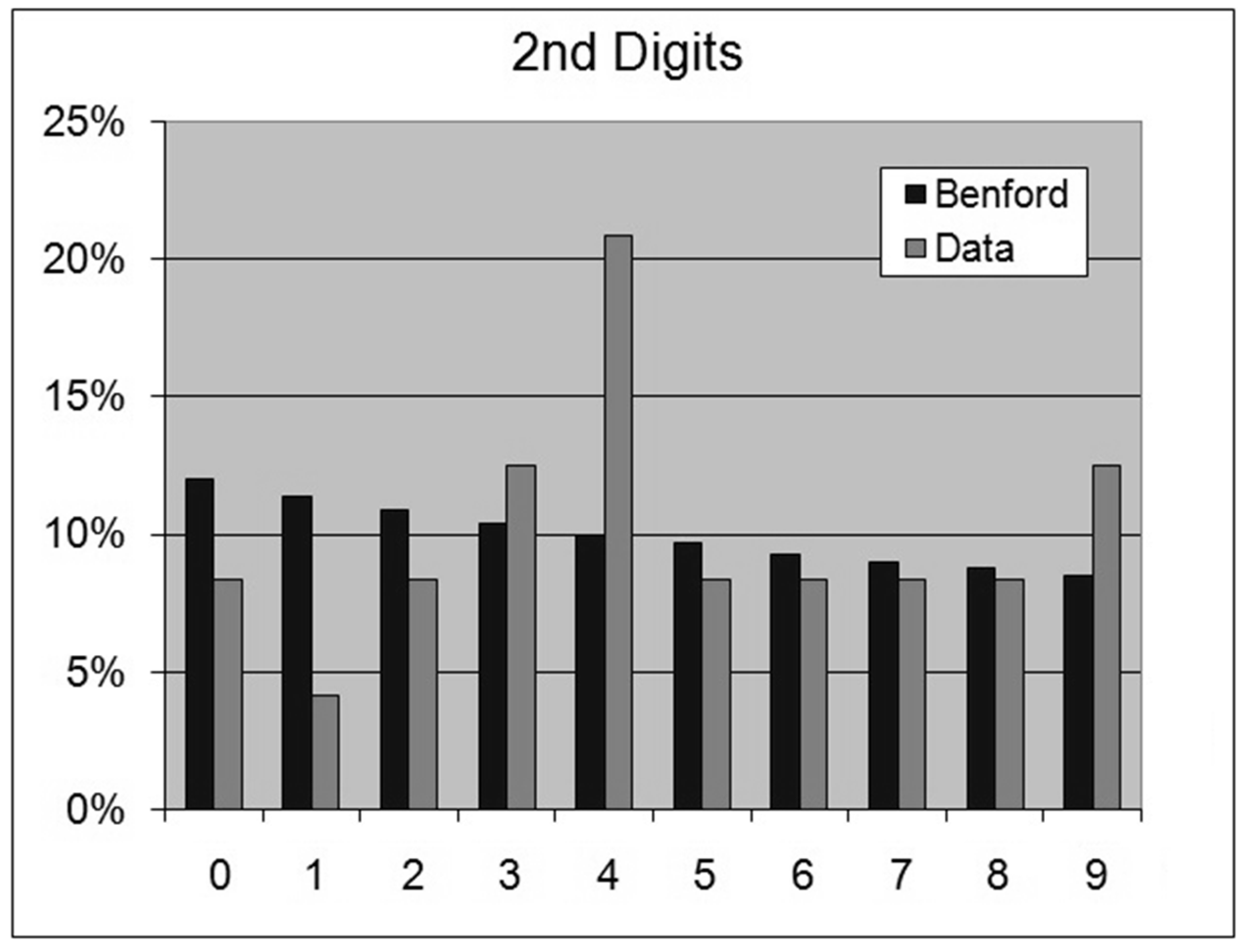
Figure 1 depicts the collection of this small sample of 40 numbers.
Figure 2 emphasizes in bold and black color the 1st digits of these 40 numbers.
Clearly, for this very small sample, low digits occur by far more frequently on the first position than do high digits. A summary of the digital configuration of the sample is given as follows:
| Digit Index: | {1, 2, 3, 4, 5, 6, 7, 8, 9} |
| Digits Count totaling 40 values: | {15, 8, 6, 4, 4, 0, 2, 1, 0} |
| Proportions of Digits with “%” sign omitted: | {38, 20, 15, 10, 10, 0, 5, 3, 0} |
One may conclude with the phrase “Not all digits are created equal”, or rather “Not all first digits are created equal”, even though this seems to be contrary to intuition and against all common sense.
2. Benford’s Law and the Predominance of Low Digits
Benford’s Law states that:
| Probability[First Leading Digit is d] = LOG10(1 + 1/d) |
| LOG10(1 + 1/1) = LOG(2.00) | = | 0.301 |
| LOG10(1 + 1/2) = LOG(1.50) | = | 0.176 |
| LOG10(1 + 1/3) = LOG(1.33) | = | 0.125 |
| LOG10(1 + 1/4) = LOG(1.25) | = | 0.097 |
| LOG10(1 + 1/5) = LOG(1.20) | = | 0.079 |
| LOG10(1 + 1/6) = LOG(1.17) | = | 0.067 |
| LOG10(1 + 1/7) = LOG(1.14) | = | 0.058 |
| LOG10(1 + 1/8) = LOG(1.13) | = | 0.051 |
| LOG10(1 + 1/9) = LOG(1.11) | = | 0.046 |
| | --------- |
| | 1.000 |
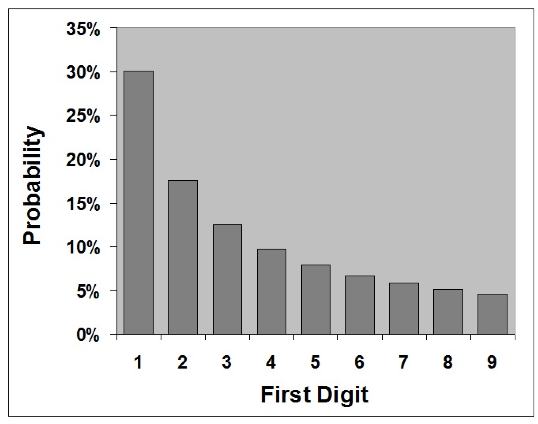
The following vector expresses the (probabilistically) expected digit proportions according to Benford’s Law—referring to the ranked digits 1 through 9:
{30.1%, 17.6%, 12.5%, 9.7%, 7.9%, 6.7%, 5.8%, 5.1%, 4.6%}.
Typically this is written as:
{30.1, 17.6, 12.5, 9.7, 7.9, 6.7, 5.8, 5.1, 4.6} with “%” sign omitted.
At times this is written as:
{0.301, 0.176, 0.125, 0.097, 0.079, 0.067, 0.058, 0.051, 0.046} being expressed as proportions or probabilities.
Figure 3 depicts the graph of the Benford distribution for 1st digits. Remarkably, Benford’s Law is found to be valid either nearly exactly so or approximately so in almost all real-life data sets, such as data relating to physics, chemistry, astronomy, economics, finance, accounting, geology, biology, engineering, governmental census data, and many others. As such Benford’s Law constitutes perhaps the only common thread running through and uniting all scientific disciplines.
Ref. [
1] provides the first influential article published on the topic. Ref. [
2] provides a comprehensive expose on the phenomenon, while [
3] provides the most recent research results in this field. Refs. [
4,
5] provide the first ever practical applications of Benford’s Law. Ref. [
6] provides a radically new quantitative vista for this seemingly mere digital phenomenon, leading to the more inclusive mathematical expression, which is termed as “The General Law of Relative Quantities” or as its acronym GLORQ.
Figure 4 summarizes the relationship between the old law and the new law, namely that Benford’s Law can be mathematically derived from GLORQ. The reference [
7] presents a more concise account of GLORQ.
3. Second Digits, Third Digits, and Higher Order Digits
Benford’s Law also gives considerations to higher order digit distributions, in addition to the 1st digit order. Assuming the standard base 10 decimal number system for example, then the 2nd leading digit (2nd from the left) of 7834 is digit 8, of 0.03591 it’s digit 5, and of 4093 it’s digit 0. The 3rd leading digit (3rd from the left) of 3271 is digit 7. For all higher orders, digit 0 is also included in the distributions, but digit 0 is not part of the 1st order.
The unconditional probabilities according to Benford’s Law for the 2nd, 3rd, and 4th orders are:
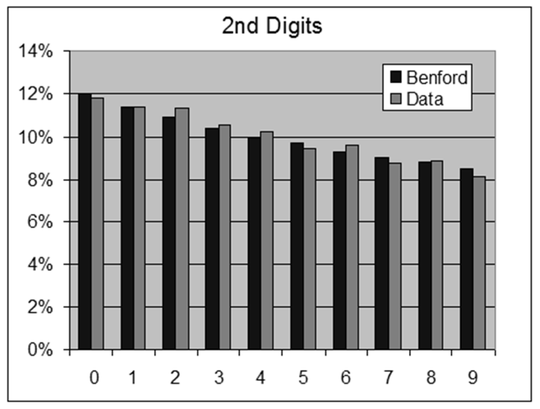
2nd Digits—{11.97, 11.39, 10.88, 10.43, 10.03, 9.67, 9.34, 9.04, 8.76, 8.50}
3rd Digits—{10.18, 10.14, 10.10, 10.06, 10.02, 9.98, 9.94, 9.90, 9.86, 9.83}
4th Digits—{10.02, 10.01, 10.01, 10.01, 10.00, 10.00, 9.99, 9.99, 9.99, 9.98}
Digit distribution for the 2nd order is only slightly skewed in favor of low digits, as opposed to the much more dramatic skewness of the 1st digit order where digit 1 is about 6 times more likely than digit 9. Digit distribution for the 3rd order shows only tiny deviations from the 10% possible equality. As even higher orders are considered, digits rapidly approach digital equality for all practical purposes, attaining the uniform and balanced 10% proportions for all the 10 possible digits 0 to 9.
4. A Robust Measure of Order of Magnitude (ROM)
Rules regarding expectations of compliance with Benford’s Law rely heavily on measures of order of magnitude of data, namely on its variability and spread. Order of magnitude of a given data set is defined as the decimal logarithm of the ratio of the maximum value to the minimum value. The data set is assumed to contain only positive numbers greater than zero.
In order to avoid outliers, preventing them from overly influencing the numerical measure of data variability, this author suggests a more robust measure with the simple modification of eliminating any possible outliers on the left for small values and on the right for big value. This is accomplished by narrowing the focus exclusively onto the core 98% part of the data. The measure shall be called Robust Order of Magnitude and it is defined as follows:
The definition simply reformulates OOM by substituting the 1st percentile (in symbols P1%) for the minimum, and by substituting the 99th percentile (in symbols P99%) for the maximum.
5. Two Essential Requirements for Benford Behavior
One of the two essential requirements or conditions for data configuration with regards to compliance with Benford’s Law is that the value of the (robust) order of magnitude of the data set should be approximately over 3. The usage of ROM as opposed to OOM guarantees that the thorny issue of outliers and edges would not be ignored.
Actually, even lower ROM values such as 2.8 and 2.5 are expected to yield Benford in the approximate, but falling below 2.5 does not bode well for getting anywhere near the Benford distribution.
Skewness of data where the histogram comes with a prominent tail falling to the right is the second essential criterion necessary for Benford behavior. Indeed, most real-life data sets are generally positively skewed in the aggregate, so that overall, their histograms come with a tail falling on the right, and consequently the quantitative configuration is such that the small is numerous and the big is rare, hence low first digits decisively outnumber high first digits.
The asymmetrical, Exponential, Lognormal, k/x (and many other distributions) are typical examples of such quantitatively skewed configuration, and therefore they are approximately, nearly, or exactly Benford, respectively. The symmetrical Uniform, Normal, Triangular, Circular-like, and other such distributions are inherently non-Benford, or rather anti-Benford, as they lack skewness and do not exhibit any bias or preference towards the small and the low.
Symmetrical distributions are always non-Benford, no matter what values are assigned to their parameters. By definition they lack that asymmetrical tail falling to the right, and such lack of skewness precludes Benford behavior regardless of the value of their order of magnitude. Order of magnitude simply does not play any role whatsoever in Benford behavior for symmetrical distributions. For example, first digits of the Normal(1035, 108) or the Uniform(1, 1027) are not Benford at all, and this is so in spite of their extremely large orders of magnitude. In summary: Benford behavior in extreme generality can be found with the confluence of sufficiently large order of magnitude together with skewness of data—having a histogram falling to the right. The combination of skewness and large order of magnitude is not a guarantee of Benford behavior, but it is a strong indication of likely Benford behavior under the right conditions. Moderate (overall) quantitative skewness with a tail falling too gently to the right implies that digits are not as skewed as in the Benford configuration. Extreme (overall) quantitative skewness with a tail falling sharply to the right implies that digits are severely skewed, even more so than they are in the Benford configuration.
6. Three Generic Causes of the Benford Phenomenon
(I) Multiplication Processes
As a general rule, Benford digital configuration and positive quantitative skewness is expected to be found in the natural sciences and in any data type whenever “the randoms are multiplied”. More specifically, the multiplicative process needs to be carefully scrutinized to determine whether there are sufficiently many multiplicands, or that at least there is sufficiently high order of magnitude within the constituent distributions. The crucial factor here is the resultant order of magnitude of the entire multiplicative process, which depends on the individual orders of magnitude of the distributions being multiplied, as well as on the number of distributions involved.
(II) Random Quantitative Partitions
Random Quantitative Partition Models lead to an approximate, nearly perfect, or exact Benford behavior for the resultant set of (small) parts, as well as positive quantitative skewness, under the following five assumptions:
- (I)
given that partition is performed on the real number basis and not exclusively on integers;
- (II)
given that all partition acts are truly random;
- (III)
given that partition thoroughly breaks the original quantity into numerous parts;
- (IV)
given that each act of partition is independent and not correlated with all the previous or future acts of partitions;
- (V)
given that no artificial or arbitrary limits or rules exist, and that partition is performed totally in free style with no limitations whatsoever.
(III) Data Aggregation and Chains of Distributions
It may not be obvious, but surprisingly quite often, real-life data sets consist of numerous, smaller, and “more elemental” mini sub-sets. Therefore, a given data set which appears to exist independently as a whole, may actually be made of several data components which are aggregated in order to arrive at that larger set of data. The implication of such aggregations to quantitative skewness and digital Benford configuration is profound, since results are almost always skewed in favor of the small, with resultant histogram having a tail falling to the right. Indeed, it can be demonstrated in general that appending various data sets into a singular and much larger data set leads to quantitative skewness in favor of the small whenever these data sets start from a very low value, ideally such as 0 or 1, and terminate at highly differentiated (varying) endpoints, so that some span short intervals while others span longer intervals. Let us demonstrate this quantitative tendency in data aggregation by combining the following six imaginary data sets:
Data Set A: {2, 3, 5, 7}
Data Set B: {1, 4, 6, 9, 13, 14}
Data Set C: {2, 6, 7, 9, 11, 15, 16, 21}
Data Set D: {1, 2, 6, 8, 13, 14, 19, 23, 25}
Data Set E: {3, 4, 8, 12, 15, 19, 22, 24, 29, 35, 41}
Data Set F: {1, 5, 8, 11, 12, 17, 19, 24, 27, 32, 38, 43, 47}
Such quantitative tendency or mechanism in aggregations of real-life data sets is one of the main causes and explanations of the Benford’s Law phenomenon in the real world. Formalism in mathematical statistics draws inspiration from such types of data compilation and points to a slightly different abstract process coined as “Chain of Two Uniform Distributions”, namely the statistical chain Uniform(min, Uniform(maxA, maxB)), where min < maxA < maxB.
The chain of distributions concept is successfully generalized from the Uniform Distribution to all types of statistical distributions, such as Exponential(Exponential(Exponential(7))) or Exponential(Normal(Uniform(15, 21), 3)), among infinitely many other chaining possibilities.
This author’s 1st conjecture is that an infinitely long chain of distributions should obey Benford’s Law exactly. Scale parameters, such as λX or X/λ (divisions and multiplications), as well as location parameters, such as X—μ (subtractions), usually respond vigorously to chaining, prefer the small over the big, and obey Benford’s Law (i.e., chain-able). Shape parameters, such as Xk (powers), usually do not respond to chaining at all, show no preference for the big, for the small, or for any size, and disobey Benford’s Law (i.e., not chain-able).
More precisely, a parameter that does not continuously involve itself in the expression of centrality (such as the mean, median, or midpoint) is not chain-able at all; and a parameter that does continuously involve itself in the expression of centrality is indeed chain-able.
The meaning of the phrase “not continuously involved” is that the partial derivative ∂(center)/∂(parameter) goes to 0 in the limit for high values of the parameter, namely that centrality such as the average, the median, and resultant range in general, are not affected as parameter is further increased, and that beyond a certain limit the parameter does not sway centrality.
Hence, if a parameter does not play any role in the determination of centrality and in the span of the range beyond the initial few low values then it’s not chain-able at all. Since most scale and location parameters (continuously) play significant role in centrality, they are generally chain-able. Since most shape parameters do not play any role in centrality in the limit, they are generally not chain-able.
In addition, a 2nd conjecture in made, predicting the manifestation of Benford’s Law exactly for the very short chain of distributions with even just 2 sequences, assuming the chain uses a distribution which obeys Benford’s Law for the inner-most parameter in its ultimate sequence.
In extreme generality and concisely in symbols, the 2nd conjecture states that:
A related extrapolation of the 2nd conjecture states that with each new added sequence (elongating the chain), the chain evolves and becomes even skewer, as well as becoming a notch closer to the digital configuration of Benford’s Law. Ref. [
8] provides rigorous mathematical proofs of the connection between chains and Benford’s Law.
7. The Chi-Square Test in the Context of Benford’s Law
It had become a dogma or rather an impulsive ritual in the field of Benford’s Law to rush into the chi-square test for whatever data set the researcher is considering, regardless of its true applicability. This erroneous groupthink has become also prevalent even in the Benford’s Law analysis of purely mathematical entities and deterministic series, which have no relationship whatsoever to randomness and probability theory. The mistaken use of the chi-square test has led to much confusion and many errors, and has done a lot in general to undermine trust and confidence in the whole discipline of Benford’s Law.
Let us narrate the definition of the chi-square statistic and its related test:
Theoretical=The expected Benford proportion for any particular digit
Theoretical 1st = {0.301, 0.176, 0.125, 0.097, 0.079, 0.067, 0.058, 0.051, 0.046}
Theoretical 2nd = {0.120, 0.114, 0.109, 0.104, 0.100, 0.097, 0.093, 0.090, 0.088, 0.085}
Observed = The observed actual proportion for the particular digit in the data set
N = The number of data points (i.e., the size of the data set)
where the summation runs from 1 to 9 for the first digits, and from 0 to 9 for the second digits.
Reject the Null Hypothesis H0 that the data set is authentically Benford at the p% confidence level if the chi-square statistic is larger than chi-square p% critical (threshold) value with 8 degrees of freedom for the 1st digits, or with 9 degrees of freedom for the 2nd digits.
The cutoff point or threshold value for the chi-square distribution, separating the probable from the improbable, is as follows:
For 1st digits:
The probability of the chi-square distribution with 8 degrees of freedom being greater than 15.5 is less than 5%.
For 2nd digits:
The probability of the chi-square distribution with 9 degrees of freedom being greater than 16.9 is less than 5%.
The Sum of Squared Deviations (SSD) measure is defined as:
8. The First Paradox
Brief descriptions of six data sets wrongly rejected as non-Benford by the chi-square test:
- (1)
Time in seconds between the 19,451 Global Earthquakes during 2012;
- (2)
USA Cities and Towns in 2009—19,509 Population Centers;
- (3)
Canford PLC Price List, Oct 2013—15,194 items for sale;
- (4)
48,111 Star Distances from the Solar System, NASA;
- (5)
Biological Genetic Measure—DNA V230 Bone Marrow—91,223 data points;
- (6)
Oklahoma State 986,962 positive expenses below $1 million in 2011.
The above six data sets are truly excellent real-life Benford examples, where the digital phenomenon manifests itself decisively, for the 1st digit distribution as well as for the 2nd digit distribution, yet, the chi-square test claims that they are not complying with the law of Benford. The very low values of the Sum of Squared Deviations (SSD) measure for these data sets reinforce the impression that digit distributions are indeed very near the Benford proportions. These six data sets are excellent representatives of the phenomenon, with deep loyalty to Benford’s Law, yet all are being betrayed by the chi-square test. This author, after having the experience of working for many years with real-life data sets in conjunction with the Benford phenomenon, can earnestly testify to the fact that these six data sets are ones of the most typical and authentic manifestation of the phenomenon; and that it would be simply wishful thinking to look for some phantom “more-Benford-like” real-life data sets with the same types of low SSD values that would miraculously manage to pacify the chi-square test and convince it to grant them acceptance as Benford (lest we superficially limit ourselves to dealing only with small data sets with low size N, which are statistically less stable and less meaningful). In sharp contrast to the challenges and difficulties of real-life random data in dealing with the highly demanding chi-square test, acceptance from the chi-square test can occur easily for abstract and theoretical entities such as the Lognormal distribution, the Fibonacci series, Exponential Growth Series, and so forth. The rejection of these six real-life data sets by the chi-square test is a strong indication that in the context of real-life practical data, the chi-square approach is profoundly problematic and misleading for many data sets, and that the whole theoretical basis of applying it needs to be reexamined carefully.
The link sources of the six data sets (all accessed on 1 April 2021) are as follow:
The 1st digit distributions of these six data sets are:
| (1) | 29.9% | 18.8% | 13.5% | 9.3% | 7.5% | 6.2% | 5.8% | 4.8% | 4.2% |
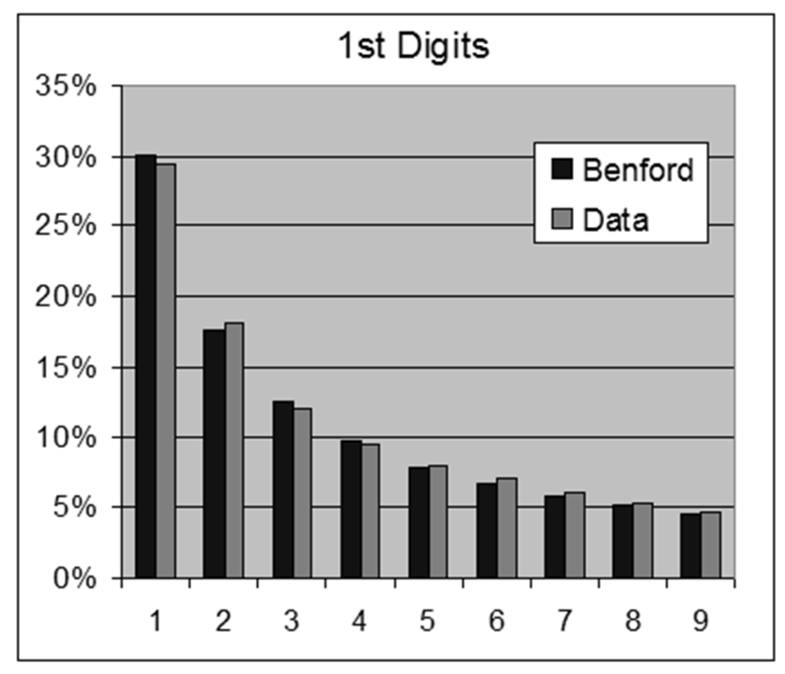
| (2) | 29.4% | 18.1% | 12.0% | 9.5% | 8.0% | 7.0% | 6.0% | 5.3% | 4.6% |
| (3) | 28.8% | 17.7% | 14.2% | 9.2% | 8.1% | 7.0% | 5.3% | 5.1% | 4.6% |
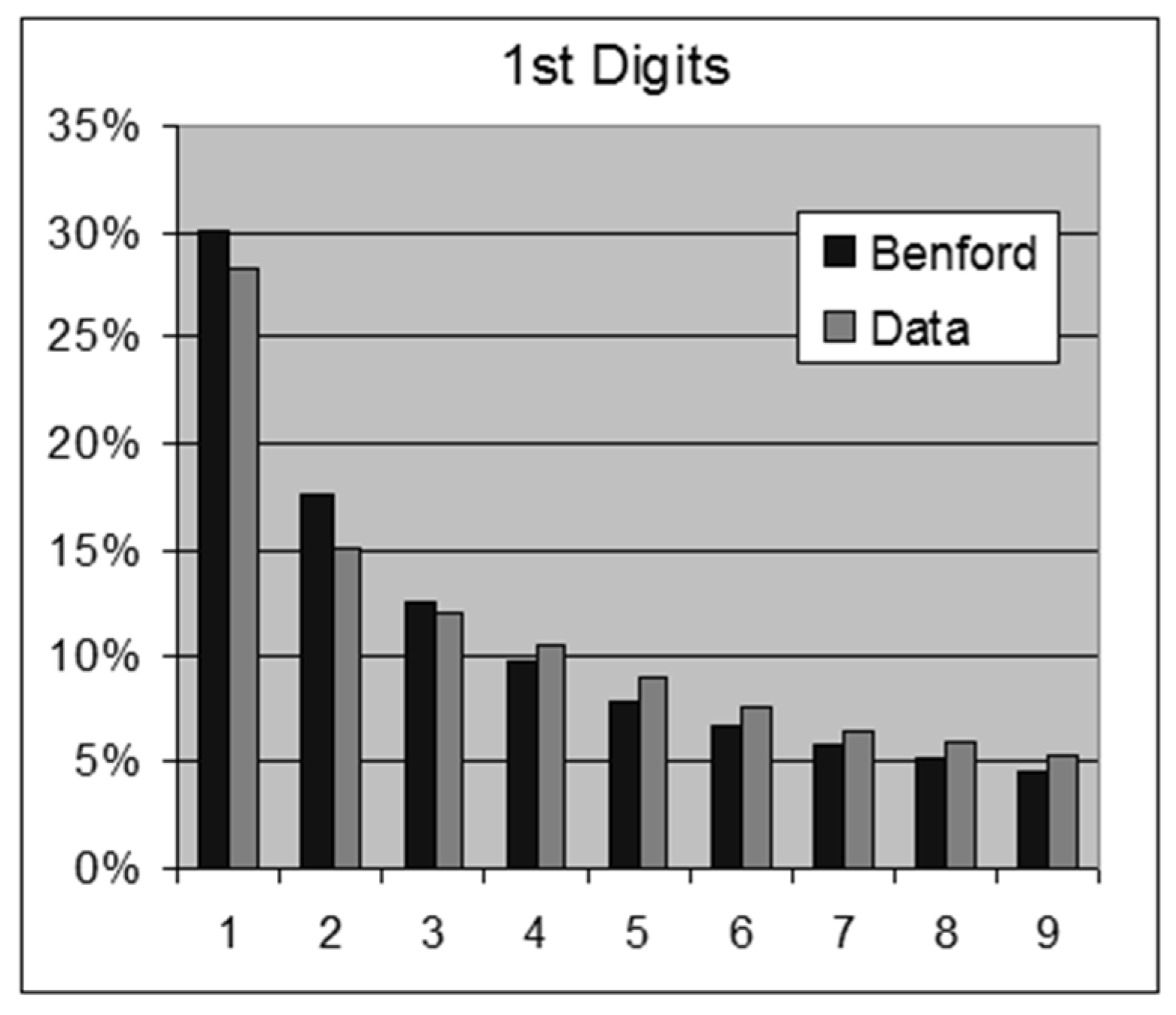
| (4) | 28.3% | 15.1% | 12.0% | 10.5% | 9.0% | 7.6% | 6.5% | 5.9% | 5.2% |
| (5) | 29.7% | 18.2% | 12.5% | 9.9% | 7.7% | 6.6% | 5.8% | 5.0% | 4.5% |
| (6) | 29.7% | 17.7% | 12.1% | 9.7% | 8.6% | 6.6% | 6.1% | 4.9% | 4.5% |
| Ben | 30.1% | 17.6% | 12.5% | 9.7% | 7.9% | 6.7% | 5.8% | 5.1% | 4.6% |
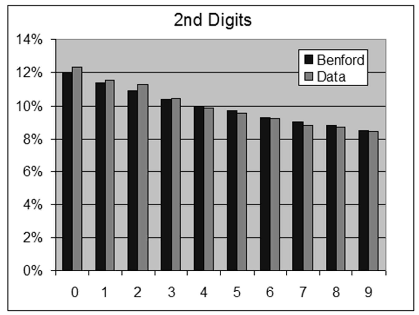
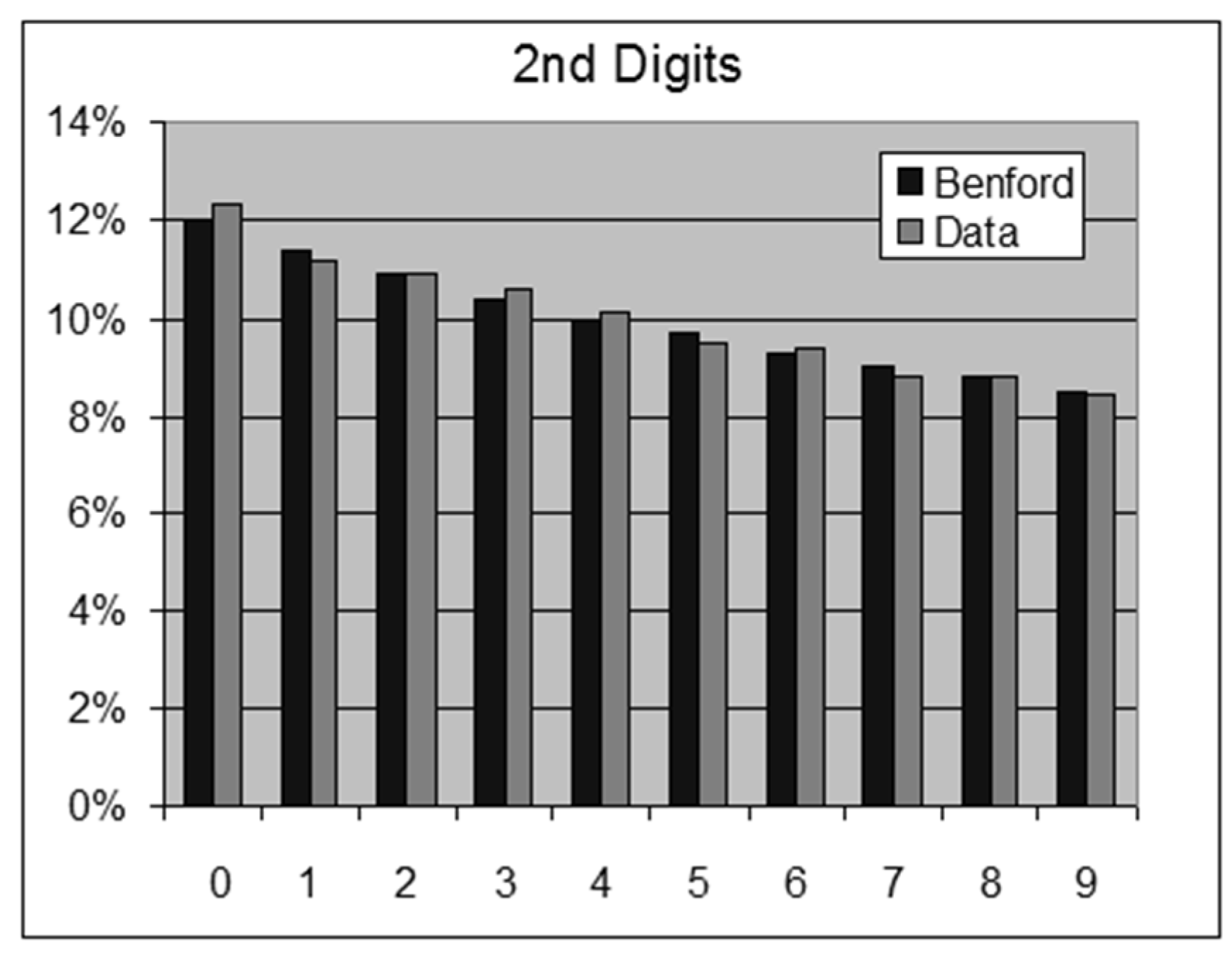
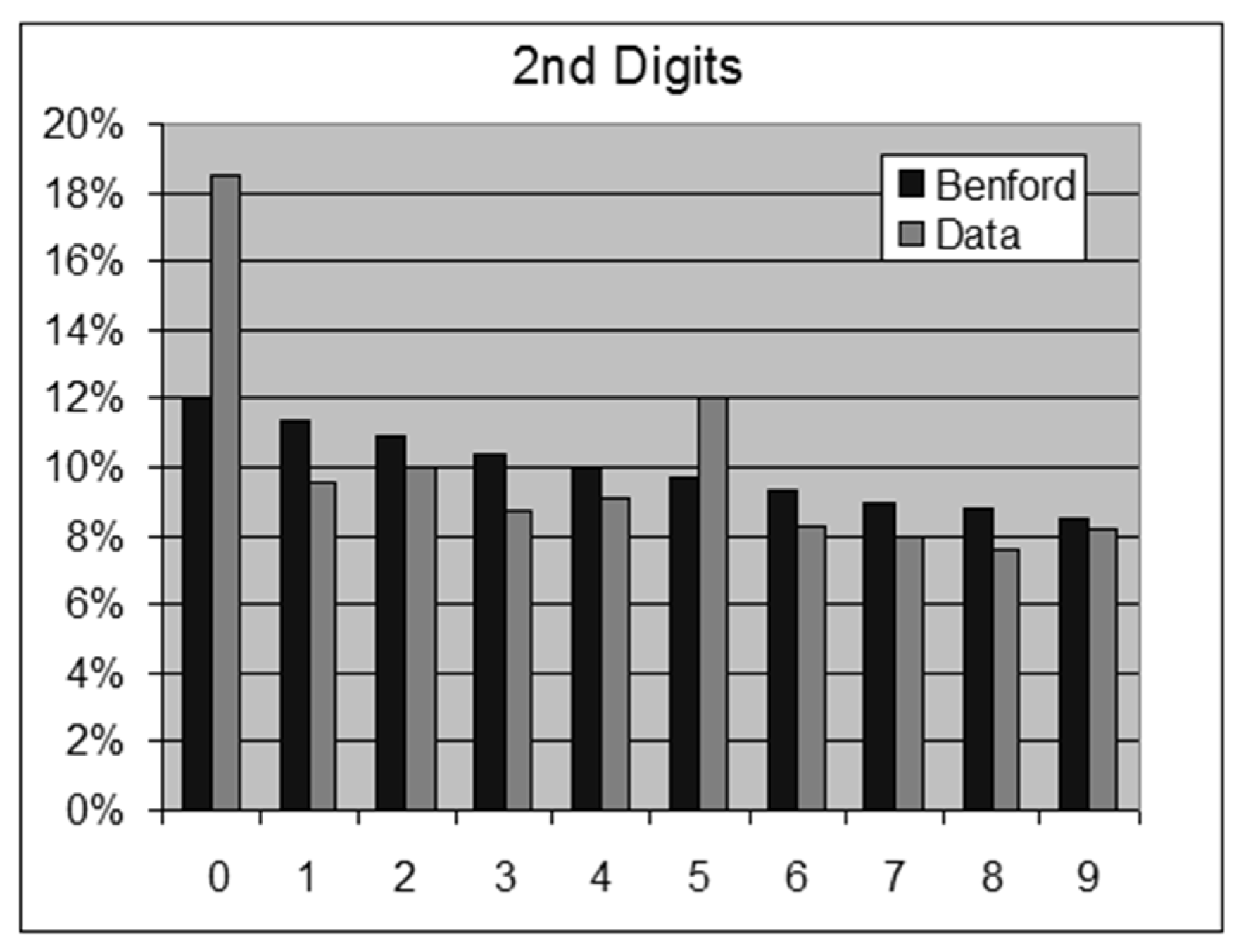
The twelve figures from
Figure 5,
Figure 6,
Figure 7,
Figure 8,
Figure 9,
Figure 10,
Figure 11,
Figure 12,
Figure 13,
Figure 14,
Figure 15 and
Figure 16 depict the graphs of the first and the second digits respectively of the six data sets mentioned above in exact sequential order.
- (1)
Time in seconds between the 19,451 Global Earthquakes during 2012.
For this data set we obtain the following results:
1st Digits: SSD = 3.1 chi-square = 53.1 > 15.5 (rejection)
2nd Digits: SSD = 0.7 chi-square = 14.0
- (2)
USA Cities and Towns in 2009—19,509 Population Centers.
For this data set we obtain the following results:
1st Digits: SSD = 1.3 chi-square =17.4 > 15.5 (rejection)
2nd Digits: SSD = 0.7 chi-square =13.1
- (3)
Canford PLC Price List, Oct 2013—15,194 items for sale.
For this data set we obtain the following results:
1st Digits: SSD = 5.3 chi-square = 57.7 > 15.5 (rejection)
2nd Digits: SSD = 6.3 chi-square = 100.6 > 16.9 (rejection)
- (4)
48,111 Star Distances, NASA.
For this data set we obtain the following results:
1st Digits: SSD = 14.1 chi-square = 538.1 > 15.5 (rejection)
2nd Digits: SSD = 0.4 chi-square = 17.7 > 16.9 (rejection)
- (5)
Biological Genetic Measure—DNA V230 Bone Marrow—91,223 data points.
For this data set we obtain the following results:
1st Digits: SSD = 0.6 chi-square = 34.7 > 15.5 (rejection)
2nd Digits: SSD = 0.3 chi-square = 27.3 > 16.9 (rejection)
- (6)
Oklahoma State 986,962 expenses below $1 million in 2011.
For this data set we obtain the following results:
1st Digits: SSD = 0.9 chi-square = 978.4 > 15.5 (rejection)
2nd Digits: SSD = 426.4 chi-square = 406,262.8
The 2nd digits of the Oklahoma expense data are excused from Benford behavior due to many typical round prices such as $7.00, $9.50, $30.00, which exaggerate digits 0 and 5 occurrences.
9. The Second Paradox
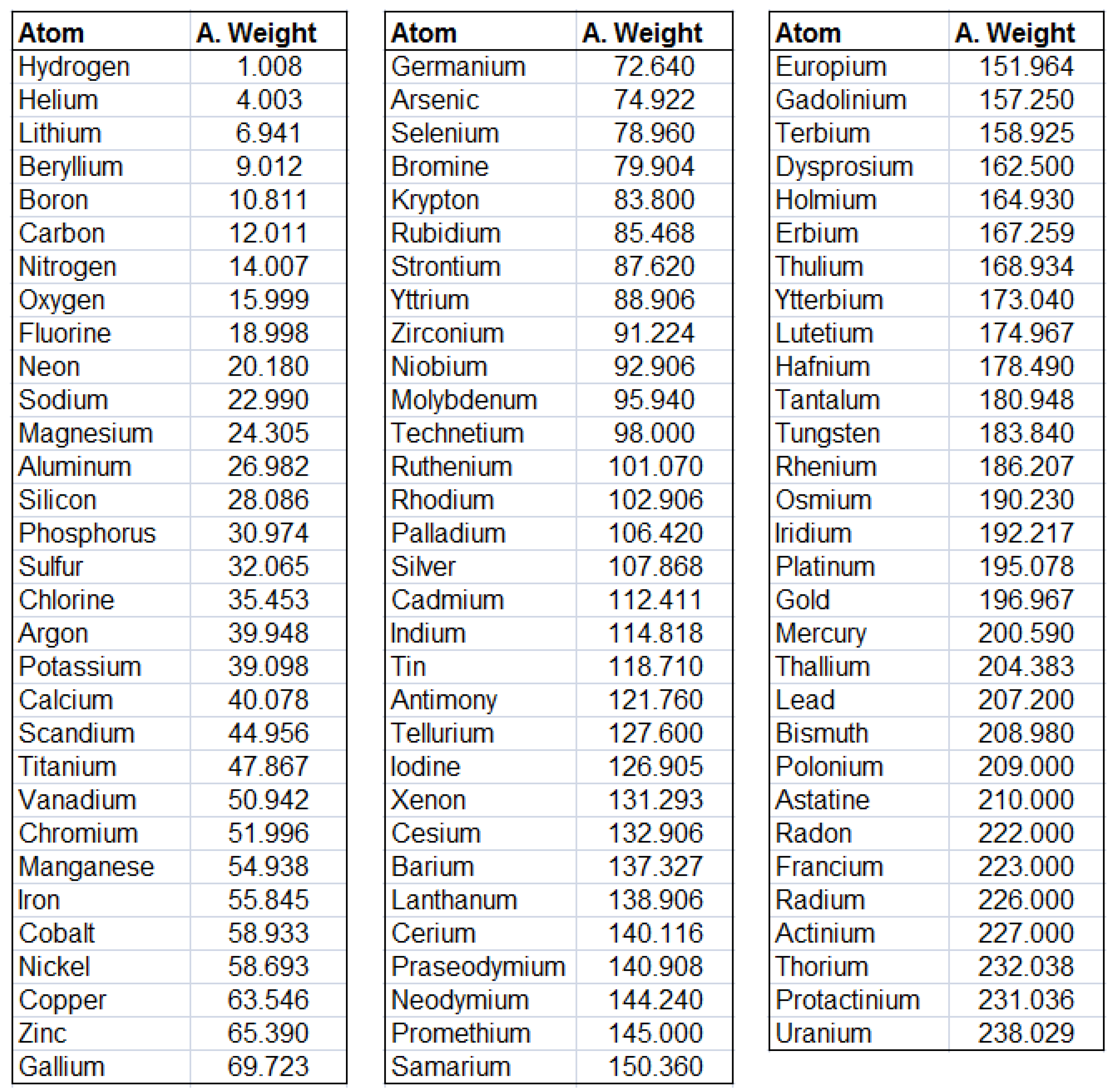
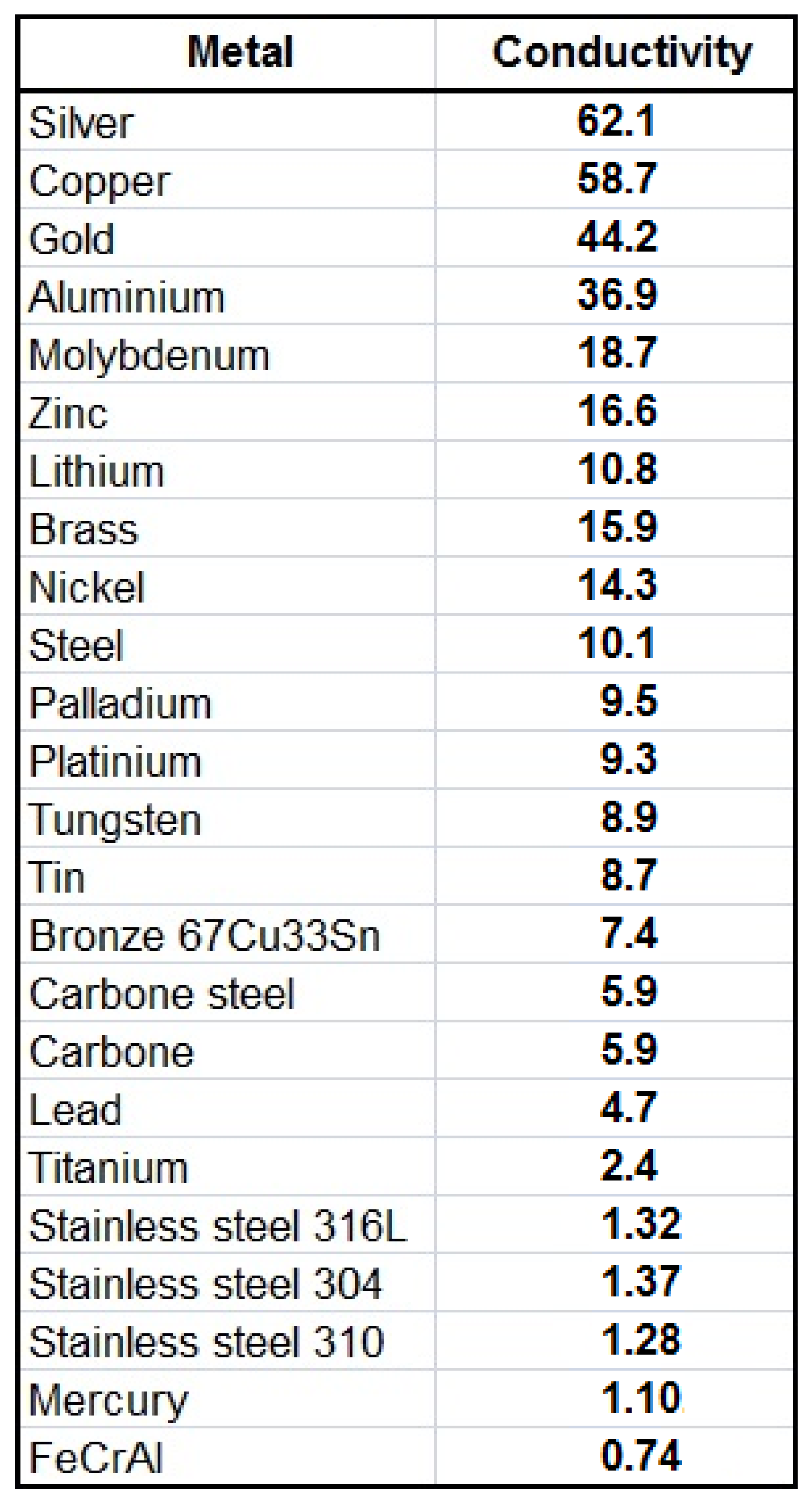
The following two data sets (regarding Atomic Weights and Metals Electric Conductivity) are approved as Benford by the chi-square test, even though they do not appear to fit the Benford configuration at all. Surely, due to the highly deterministic, exact, and scientific way these data values are chosen by Mother Nature, there is nothing random or statistical about these two lists of numbers, hence the application of the chi-square test in the cases of these two particular data sets cannot be justified in the least.
The high values of the Sum of Squared Deviations (SSD) measure here reinforce the impression that digit distributions here are indeed nowhere near the Benford proportions. All this is another strong indication that in the context of real-life practical data, the application of the chi-square test is indeed problematic and misleading for the majority of data sets.
- (1)
List of 92 Atomic Weights in the Periodic Table, from Hydrogen to (and including) Uranium, as depicted in the table of
Figure 17.
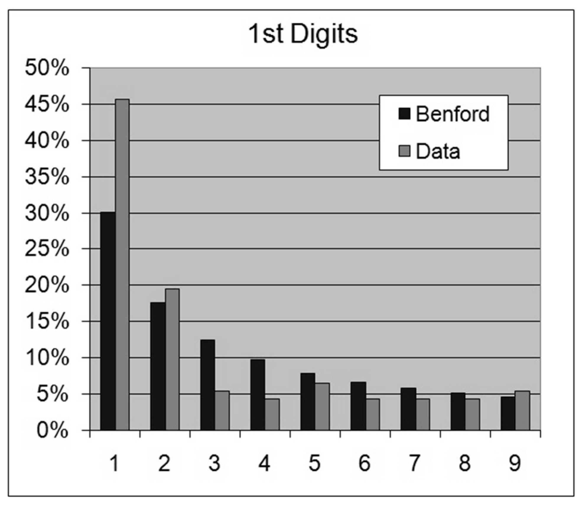
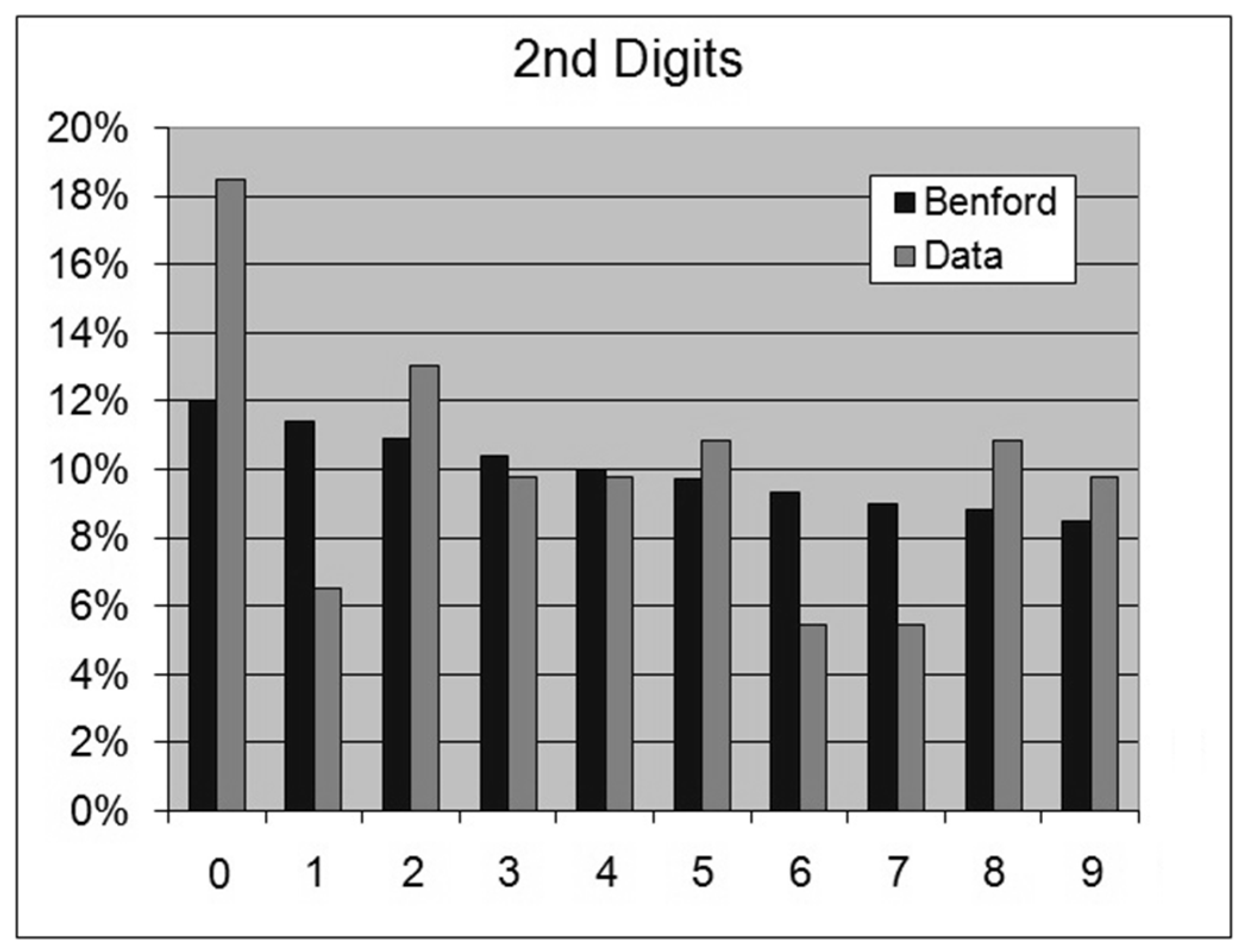
Figure 18 and
Figure 19 depict the graphs of the first and second digits respectively for the Atomic Weights data. See
https://www.webelements.com/ (accessed on 1 April 2021) for a concise summary.
For this data set we obtain the following results:
1st Digits: SSD = 334.9 chi-square ≈ 15.5 = 15.5 (borderline acceptance)
2nd Digits: SSD = 105.7 chi-square = 9.1 < 16.9 (acceptance)
- (2)
List of Electric Conductivity Values (in 1,000,000 Siemens/meter) for 24 Common Metals, as depicted in table of
Figure 20.
Figure 21 and
Figure 22 depict the graphs of the first and second digits, respectively, for the Metals Electric Conductivity data. The link
https://www.tibtech.com/conductivite (accessed on 1 April 2021) provides a concise source of the data.
For this data set we obtain the following results:
1st Digits: SSD = 443.9 chi-square = 7.3 < 15.5 (acceptance)
2nd Digits: SSD = 213.6 chi-square = 5.0 < 16.9 (acceptance)
10. The Proper Use and Context of the Chi-Square Application
Supposedly, long ago in the 1950s or in the 1960s, when the field of Benford’s Law had just started developing, one author perhaps, possibly writing a very short article focusing on a particular aspect of Benford’s Law, or writing on one particular manifestation of the phenomenon with a good fit to the Log(1 + 1/d) proportions, jumped and erred in adapting the chi-square statistic as a proper test, without much thought or self-criticism. Later perhaps, other authors with 10-page or 15-page short articles, who had possibly noticed that first erroneous article, mindlessly copied the chi-square idea. Those later researchers were without any deep interest in the field, having only a narrow focus on another manifestation or aspect of it. Others consequently then copied them as well, and so forth, until it had become a groupthink and a well-established dogma in the field.
Let us self-contemplate about digital tests in extreme generality. With regard to any particular data set on hand in the context of Benford’s Law analysis, there is a strong need to conceptually differentiate between two very different research questions here, namely between compliance and comparison.
The term compliance would refer to an attempt to answer the typical question asked by the anxious auditors, digital analysts, statisticians, fraud detectors, and researchers, once all digit distributions regarding the data set in question are obtained and clearly displayed, namely: “Does the data obey Benford’s Law or not?” Or equivalently asking the simpler question: “Is the data set Benford or not?” This is “yes or no”, “black or white”, “right or wrong”, type of a question.” As if there is no middle ground. Alternatively, we may ask the question: “Is the (tiny or mild) digital deviation from Benford for this data set due merely to chance and randomness or is it structural?”
The term comparison would refer to a particular data set with its own particular digital configuration. When such digital result is acknowledged, accepted, and respected in its own right, as it should be, since Benford’s Law does not apply to all real-life data sets; one legitimate question could then be asked in this context, namely: “How far is the data set from Benford?” If data seems close to Benford then we might ask: “How close is the data set to Benford?”One may inquire about the degree of deviation or “ A Measure of Distance from Benford”. And even though the definition chosen to accomplish this—no matter how reasonable—would still be ultimately arbitrary; yet it is altogether fitting and proper that we should construct it. Indeed, the Sum of Squared Deviations (SSD) measure could serve as an excellent comparison definition!
It is important to understand the underlying assumptions and background of the chi-square test regarding compliance. The chi-square test refers to a sample of size N, randomly taken from an infinite population assumed to have the Benford property exactly. In addition, it is assumed that we patiently and calmly select those N values in a process by which each value is chosen totally independent from each other. We close our eyes and pick, one by one, from a huge pool of Benford numbers where each number has a unique first digit out of 9 digital possibilities, and that each selection or sampling is independent of all the past and future selections and samplings. The long and complex act of randomly selecting those N values, one-by-one, from that huge Benford pool of numbers, is truly deserving of the term “Process”.
The inference and the focus here is not about the population’s Benford property, which is taken as a given, but rather about the digital property and the integrity of the list of samples on hand (i.e., the given data set). A large deviation from Benford for large enough sample size is presumed to indicate an error, bad sampling procedure, or at the least a mishap of sorts, and possibly an evidence of intentional manipulation as in outright fraud.
Analyzing a piece of data digitally, with the intended purpose of determining compliance with Benford, implicitly implies that we are comparing this particular piece of data with some generic and larger population universe already known to be Benford. Say we have 57,000 revenue transactions from IBM relating to the first quarter of 2008. We are trying to investigate whether or not IMB gave honest information, and so 1st digits distribution is studied compared to Benford, and a decisive conclusion regarding honest/fraudulent reporting by IBM is arrived at via the chi-square test. Implicit in this whole forensic scheme is that the universe of revenue amounts, relating to all companies around the globe, obeys Benford’s Law, and which is indeed assumed to be true at least by this author (after working for many years with revenue and expense data and finding nearly all individual accounting data sets of large sizes to obey Benford’s Law). Surely, the hourly revenue of a tiny coffee shop on a street corner with a tiny clientele is not Benford, but the global aggregate—if the chief auditor at the IMF could ever obtain such enormous and confidential data—is very nearly perfectly Benford. It is only in this context that the IBM data on hand is considered a sample, namely a sample from a much larger abstract population (of the universe of revenue amounts, relating to all companies around the globe); and it is only in this context too that statistical theory can lend a hand and provides us with cutoff points and threshold values, by way of indicating their exact probabilistic significance. Yet, there is a serious pitfall in such an approach, namely that the nature of the sample data should resemble the nature of the population in all its aspects, and this is rarely so, except in the mind of the eager, ambitious, and naïve auditor or statistician seeking an error-proof algorithm capable of detecting fraud where perhaps none exists. For example, the data on hand about IBM revenues is in reality the entire population, not a sample from that imaginary “universe of revenues”. This is so since each company has its own unique price list, particular clientele, unique products for sale, and belonging to some very specific sub-industry. Alternatively stated, the particular data set on hand, even if it can be thought of as a sample, was not “taken from the larger population” in a truly random fashion. It is impossible to argue that these 57,000 revenue transactions from IBM database is a random sample from the universe of that generic and global revenue data type! To take a truly random sample from such imaginary universe/population, one should take, say only, 25 random values from IMB, 12 random values from Nokia, 17 random values from GM, and so forth, in which case results are guaranteed to be nearly perfectly Benford, and the application of the chi-square test wholly justified and workable!
An even more profound source of confusion and mistaken applications of the chi-square test in the context of Benford’s Law is the fact that frequently it is impossible to contemplate or consider some larger data type standing as the population for the data set on hand. Frequently, what we have on hand is simply a unique set of numbers pertaining to a very particular issue or process, and attempting to envision it belonging to some, “larger” or “more-generic” (and Benford) population data type is nothing but a fantasy, a misguided tendency to seek help from statistical theory where none exists. Even more incredible is to imagine the particular data set on hand as “a sample” of sorts being generated in “a truly random fashion” from that imaginary and non-existent parental universe/population!
As an example, suppose a researcher is investigating the particular phenomenon of chemical acidity in drinks. The researcher has worldwide data on all 12,658 known drinks, fruit juices, vegetable juices, alcoholic beverages, coffee, tea, potions, and so forth, exhausting all possible sources, without neglecting a single exotic drink on some far away Pacific island or those drunk during rare religious and ceremonial occasions. The pH measure of all 12,658 drinks yields a particular 1st digits distribution of say {41.8, 26.1, 5.0, 7.5, 2.4, 2.5, 3.4, 8.6, 2.7}. It does not make any statistical sense here to test about whether or not the given data set is Benford or not via the chi-square statistic (i.e., compliance). There is no null hypothesis to accept or reject. This pH data set is not a sample from some supposed larger universe/population to be compared with. Certainly, the researcher cannot claim that his/her data on hand was obtained in a “truly random fashion” from that imaginary larger population of pH values! That would border on the absurd! This pH data set stands apart, proud and independent, existing in its own right. The issue of fraud does not enter here of course, and yet, one may legitimately wonder and ask “how far is digital distribution of this pH data set from Benford” (i.e., comparison). There can’t be, and there shouldn’t be of course, any talk here of probabilistic 5% or 1% significance level, or of any supposed “chances” of obtaining such a non-Benford pH digital result. Actually, this pH example is given for pedagogical purposes only; while a more realistic digit distribution for pH values would typically be perhaps as in: {0%, 3%, 21%, 13%, 37%, 19%, 7%, 0%, 0%}, where 2.0 is just about the most acidic drink, and 7.5 about the strongest alkali.
A totally different statistical scenario is demonstrated with the example of the mid-level newly hired financial analyst or economist working at the IMF, being asked by the top director of the institution to provide two large separate samples of revenues worldwide from a large mixture of companies for the years 2007 and 2008, as a comparison in the study of the causes leading to the onset of the Great Recession. On the (correct) assumption that global revenue data truly follows Benford’s Law, the top director can discreetly perform a digital test on the data provided by the little known and newly hired employee as a check whether (I) data was seriously and correctly collected in good faith, or that (II) workload was fraudulently reduced by simply concocting invented revenue numbers by the lazy and dishonest new analyst. In this example, the statistical methodology of the chi-square test (i.e., compliance) can and should be applied by the top director in order to detect fraud (or rather to detect laziness.)
The chi-square test incorporates the term N, implying that whenever the size of the data set is quite large, even a seemingly mild deviation from Benford can still show a fairly large value of chi-square statistic, thus rejecting compliance with Benford’s Law. Because of this fact, the chi-square test is mistakenly thought to be “oversensitive”, in the sense that for large data sets (say over 25,000 values) supposedly even mild deviations from Benford are flagged as significant (“false positive”). In other words, the test is erroneously thought to suffer from excessive power. This misguided perception of “oversensitivity” is an indication that users lack understanding of the underlying statistical basis of the test.
The dignified and well-respected statistician disguised as an addicted gambler and wearing some very casual clothes, confidentially sent to an ill-reputed casino by the authorities to investigate possible dishonesty and biasness of the large die in use there, should certainly not be derogatorily referred to as “oversensitive” or as “overzealous” if he/she declares the casino to be fraudulent when after 10,000 throws of the die only 1027 times the lucky face of 6 showed up, instead of the expected 1667 times (calculated as 10,000∗(1/6)). The statistician should become increasingly overzealous and suspicious as the number of throws N increases and the ratio continues to significantly deviate from the theoretical 1/6 value. In any case, rightly or wrongly, the chi-square test nowadays is used quite frequently whenever data set is relatively small, and it is erroneously (or rather conveniently) avoided whenever data set is deemed too large. Generally, auditors (mistakenly) consider any account with over 25,000 or 50,000 entries as “too large for the chi-square test”. This is akin to the irrational critically ill patient asking the laboratory to return his/her blood tests only if results are negative and to discard the whole thing if it brings bad news. In reality, the chi-square test should usually be avoided altogether in the context of Benford’s Law and regardless of data size, due to the often questionable basis of the underpinning statistical theory. Data size should never be the basis for deciding whether to apply the chi-square test or not, rather the correctness in the modeling of the data as a truly random sample of some larger Benford population should be the only criteria of proper application.
The supposedly “troublesome” value of N is noted within the chi-square expression above as a multiplicative factor, implying that for any given magnitude of deviation (actual from expected) the statistic still depends on N and increases accordingly. When N is quite large the test seems to become “too sensitive” in the eye of the non-statistician, and bitter complaints about the N term within the algebraic expression are frequently heard, as even tiny deviations from the Benford proportions flag the data set as significantly non-Benford. While such oversensitivity is perfectly proper and statistically correct if test is applied under the right circumstances, lack of statistical understanding has caused many to misguidedly call it “false positive” and to claim that the chi-square test itself suffers from “excess power”. Yet, when data set is large, and when the underlying basis of applying the chi-square test is valid, namely that the data was drawn in a truly random fashion from a truly Benford population, the chance of finding deviations from Benford in our sample (i.e., data on hand) is closely related to data size N, and probability of even minute deviation sharply diminishes whenever size N is large.
Analogously, our statistician turned detective investigating supposed fraud by the casino owners, would accept not seeing a single face of six in 10 throws, but not if the die is thrown 1000 times all to no avail without a single face of six. This is simply the consequence of the law of large numbers. Certainly, the statistician would still certify the casino as fraudulent even if the face of six pops out, say, 50 times in 1000 throws (5%), but would not be suspicious at all if out of 10 throws the face of six never pops out (0%)! As the number of die trials increases, we demand better accuracy with that supposed 1/6 probability value (16.6%), hence for only 10 throws the low value of 0% is quite acceptable, while for 1000 throws not even 5% is enough for establishing trust, and the unbiased-ness of the die is called into serious doubt.
Since SSD does not incorporate the term N in its expression, one gets the same measure and conclusion regardless of the number of observations in the data set (i.e., its size). But this comes with a certain price, as there is no associated statistical theory to guide us. There is also no hope that future statistical studies would somehow yield threshold points, significant values, or confidence intervals by applying SSD, since those highly beneficial results would certainly require involving N somewhere in the relevant expression, while N is nowhere to be found in the definition of SSD. Statistical theory cannot be indifferent to data size N, since there is no way to tell whether a certain deviation from Benford is due to chance or to structural causes without knowing how many values have been collected as a sample from that supposedly larger Benford population universe. SSD is therefore applied only as a measure of distance from Benford, and one has to subjectively judge a given SSD value of the data on hand to be either small enough and thus somewhat close to Benford, or too high and definitely non-Benford in nature. A more systematic way of going about it is to empirically compare SSD of the data set under consideration to the list of a large variety of SSD values of other honest and relevant data sets of the same or similar type. Such accumulated knowledge helps us in empirically deciding (in a non-statistical and non-theoretical way) on the implications of those SSD values. Yet some subjectivity is unfortunately necessary here in choosing cutoff points.
Parts of the paragraphs in this chapter are found also in [
2] which is the author’s book “Benford’s Law: Theory, the General Law of Relative Quantities, and Forensic Fraud Detection Applications”, chapters 35, 36, 37, and 38. These chapters contain extended material on the topic and detailed explanations of the empirically-based cutoff points for the SSD measure.
11. The Statistical Theory Forming the Basis for the Chi-Square Test
By definition, the nature of random data yields a random first digit for each number in the data set. Evidently, the digit frequencies are explained by and are generated via some random variable or random process. Hence, whether the numbers within a given data set of size N begin or do not begin with a particular digit d is governed by a Binomial Distribution with mean Np and variance Npq, namely with mean N∗Log(1 + 1/d) and variance N∗Log(1 + 1/d)∗(1 − Log(1 + 1/d)). The Central Limit Theorem (CLT) implies that the Binomial Distribution is approximately Normal for a large value of N whenever p is not too close to either 1 or 0, namely whenever Log(1 + 1/d) is not too close to either 1 or 0. This is so since the Binomial(N, p) is the sum of N independent and identically distributed Bernoulli variables with parameter p.The above requirement for a large value of N implies that data sets with exceedingly small N value are not eligible to apply the chi-square procedure, even when data points are known to have been selected truly randomly and independently. Yet, this fact does not truly absolve the second paradox of its error.
Attention must be paid and caution exercised due to the fact that a discrete whole numbers distribution (Binomial) is being approximated by a continuous distribution (Normal) of integrals as well as fractional values, and which is a delicate, subtle, and complex endeavor, and could be quite problematic for low values of N.
Specifically the CLT shows the asymptotic (standardized) normality of the random variable:
which is distributed as the Standard Normal with mean 0 and standard deviation 1, where O is the observed number of successes in N trials (i.e., Binomial), and where the probability of success is p, and the probability of failure is q = 1 − p. Squaring both sides of the equation yields:
In mathematical statistics it is known that if Z is the Standard Normal random distribution with mean 0 and standard deviation 1, then its square Z2 is distributed according to the chi-square distribution with 1 degree of freedom. Hence the χ2 expression above is indeed chi-square 1.
Since q = 1 − p, the sum of p and q is simply 1, namely (p + q) = (p + (1 − p)) = 1.
Therefore, the above expression for
χ2 can be written as:
The expression on the right-hand side is what Karl Pearson would generalize from the Binomial to the Multinomial, and which would be written in the form:
where:
χ2 = Pearson’s cumulative test statistic, which asymptotically approaches the chi-square distribution with n Degrees of Freedom (DOF);
Oi = The number of observations of multinomial type I;
Ei = Npi = The expected theoretical frequency of multinomial type i, asserted by the null hypothesis that the fraction of multinomial type i in the population is pi;
n = The number of categories in the multinomial;
For the manifestation of Benford’s Law in data sets, these generic notations assume more specific meanings:
χ2 = The test statistic representing the chi-square with (9 − 1) or (10 − 1) DOF;
Oi = The number of values in the data set with 1st digit d, or with 2nd digit d;
Ei = N∗Log(1 + 1/d), or N times the 2nd digit Benford distribution for d;
n = 9 for the 1st digits, or 10 for the 2nd digits. But DOF is reduced by 1 to ( n−1).
The Binomial distribution may be approximated by a Normal distribution, and the square of its Standardized Normal distribution is the chi-square distribution with one degree of freedom. A similar result is obtained for the Multinomial distribution, as Pearson sought for and found a degenerate Multivariate Normal approximation to the Multinomial distribution. Pearson showed that the chi-square distribution arose from such a Multivariate Normal approximation to the Multinomial distribution.
The main fallacy of applying the chi-square test in the context of Benford’s Law is that the 1st digits and the 2nd digits of typical real-life data values are not distributed as Bernoulli variables, all with identical p value—even within a single data set. Moreover, this author as Benford’s Law researcher and data scientist (surely to be collaborated by other data analysts) is well-aware of the notion that the 1st digits and the 2nd digits of data values very rarely or almost never occur truly independently of each other, and are not separately selected or created out of thin air as independent and identical Bernoulli variables. Thus, the entire set of all the 1st digits and all the 2nd digits of the data values cannot be declared as constituting a truly Multinomial Distribution. Consequently, the entire edifice forming the basis for the chi-square test outlined above falls apart.
12. Comparison of the Chi-Square Statistic with SSD
The SSD measure is originally expressed in percent format, such as 30.1, as opposed to fractional/proportional format, such as 0.301, hence the factor of 1002 or simply (100) × (100) scale in the above expression is derived from the scale conversion (0.301) × (100) = 30.1.
The SSD measure could be thought of as the square of the Euclidean distance in R9 space, namely the square of the “distance” from the Benford point to the data digital point.
As was shown in the previous chapters, the chi-square test has no statistical or probabilistic validity in nearly all cases of real-life data sets; hence, the search for the most reasonable measure of comparison would lead us to choose freely between SSD and the chi-square statistics, among other possible constructs perhaps. In this chapter we demonstrate that SSD is a much superior choice as compared with the chi-square alternative, even when N is being fixed at a constant level so as not to be a factor in the considerations. SSD will be shown as a thorough and complete measure of distance, and this acknowledgement eliminates the motivation for the search of (supposedly “more ideal”) alternative possibilities, such as chi-square, or chi-square/N, or the sum of 9 absolute values of deviations, and so forth.
The chi-square statistic divides each deviation-square by the theoretical expectation, namely dividing each deviation-square by LOG(1 + 1/d) for the 1st digits, all of which results in the amplification of the deviation-square for digit 1 only by 1/(0.301) = 3.32, and the amplification of the deviation-square for digit 9 by the much bigger factor of 1/(0.046) = 21.85. Hence, the chi-squared statistic overemphasizes fluctuations for high digits, such as {7, 8, 9}, and it deemphasizes fluctuations for low digits, such as {1, 2, 3}.
Admittedly, the absolute values of the fluctuations associated with the high digits, say {7, 8, 9} are often much smaller than those associated with the low digits, say {1, 2, 3}. Hence, the equitable or fair philosophy of the chi-square statistic is to pity the high digits for their normally smaller fluctuations around LOG(1 + 1/d), and to attempt to help them out by amplifying their deviations more so relative to low digits, so that they gain some measure of equal footing with low digits.
Yet, this is totally an unnecessary and perhaps counterproductive measure of adjustment. It should be noted that the 9 digits are all broadly connected as they all sum up to 100%. If the low digits are over their Benford usual allocations, say digit 1 with 35%, digit 2 with 20%, and digit 3 with 15%, earning together the proportion of 70%, then the rest of the digits, namely the higher digits 4 to 9, must earn only 30% in total, which is below their Benford normal allocations. In extreme generality, low digits and high digits, as two distinct groups, are very often sensitive to each other as they instinctively react to each other, and usually simultaneously move in opposite directions. Hence, there is normally no need to emphasize or deemphasize some particular digits at the expense of others. Admittedly, at times we find deviation only in low digits, or only in high digits, such as when digit 1 is given an extra 2%, while digit 2 is being reduced by 2%, or when digit 8 is given an extra 3%, while digit 9 is being reduced by 3%, yet, this author doesn’t find a compelling reason to amplify the deviations of high digits at the expense of low digits.
As opposed to the chi-square approach, the SSD measure gives all 9 digits a truly fair and equitable chance of participating in the measure of deviation from Benford, without aiding high digits at the expense of low digits.
Let us provide several specific examples which demonstrate the distinct tendencies of SSD and chi-square values. We fix the value of N at 1000 data points in all cases, and starting with the original base set of proportions of Log(1 + 1/d), we then experimentally reduce or increase the proportions for some digits up or down from that original Benfordian level:
If digit 1 is given an extra 3%, while digit 9 is being reduced by 3%, then:
{33.1, 17.6, 12.5, 9.7, 7.9, 6.7, 5.8, 5.1, 1.6} SSD = 18.0 chi-square = 22.7.
If digit 1 is given an extra 3%, while digit 7 is being reduced by 3%, then:
{33.1, 17.6, 12.5, 9.7, 7.9, 6.7, 2.8, 5.1, 4.6} SSD = 18.0 chi-square = 18.5.
If digit 1 is given an extra 3%, while digit 5 is being reduced by 3%, then:
{33.1, 17.6, 12.5, 9.7, 4.9, 6.7, 5.8, 5.1, 4.6} SSD = 18.0 chi-square = 14.4.
If digit 1 is given an extra 3%, while digit 3 is being reduced by 3%, then:
{33.1, 17.6, 9.5, 9.7, 7.9, 6.7, 5.8, 5.1, 4.6} SSD = 18.0 chi-square = 10.2.
If digit 1 is given an extra 3%, while digit 2 is being reduced by 3%, then:
{33.1, 14.6, 12.5, 9.7, 7.9, 6.7, 5.8, 5.1, 4.6} SSD = 18.0 chi-square =8.1.
For the above series of five examples, digit 1 had an increase of 3%, and therefore this must be countered via some reduction in other digits so that total is 100%. As the occurrence of the 3% reduction shifts from high digit to lower digit, chi-square is steadily being reduced, and this does not have much merit in the author’s opinion. SSD on the other hand seems to be acting more rationally and steadily, as it yields the constant 18.0 value in all five examples.
Let us consider four more examples with fixed N value of 1000 data points.
If digit 1 is given an extra 2%, while digit 9 is being reduced by 2%, then:
{32.1, 17.6, 12.5, 9.7, 7.9, 6.7, 5.8, 5.1, 2.6} SSD = 8.0 chi-square = 10.1.
If digits 1, 2, 3, 4 are each given an extra 1%, and 6, 7, 8, 9 are each being reduced by 1%, then:
{31.1, 18.6, 13.5, 10.7, 7.9, 5.7, 4.8, 4.1, 3.6} SSD = 8.0 chi-square = 10.1.
If digit 1 is given an extra 2%, while digit 2 is being reduced by 2%, then:
{32.1, 15.6, 12.5, 9.7, 7.9, 6.7, 5.8, 5.1, 4.6} SSD = 8.0 chi-square = 3.6.
If digit 8 is given an extra 2%, while digit 9 is being reduced by 2%, then:
{30.1, 17.6, 12.5, 9.7, 7.9, 6.7, 5.8, 7.1, 2.6} SSD = 8.0 chi-square = 16.6.
The chi-square statistic assigns more importance to deviations for the high digits, and it assigns by far lesser importance to deviations for the low digits. Hence the last example above with digits 8 and 9 deviating by 2% each, the chi-square attains the value of 16.6, and it rejects the distribution as non-Benford, while in the example just above that, with digits 1 and 2 deviating by 2% each, the chi-square attains the value of 3.6, and it accepts the distribution as Benford.
SSD on the other hand remains totally indifferent as to where deviations take place, treating high digits and low digits equally, as it calculates the same deviation-distance of 8.0 in both examples.
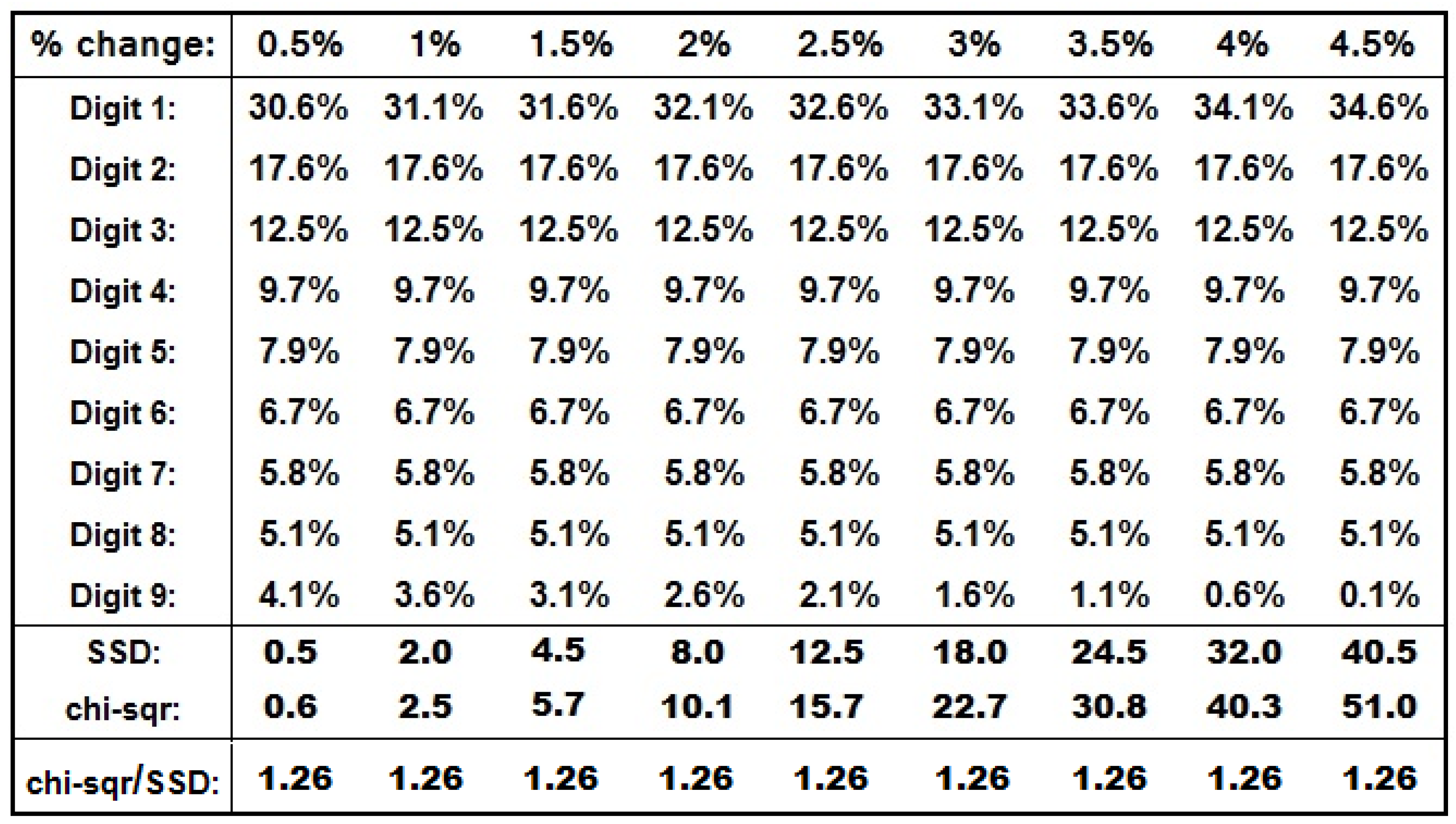
Let us provide several more examples regarding the tendencies of SSD and chi-square values. We fix the value of N at 1000 data points in all examples, and starting with the original base set of proportions of Log(1 + 1/d), we then experimentally increase the proportion of digit 1 by incremental steps of 0.5% up from the original Benfordian level, while simultaneously reducing digit 9 by these incremental steps of 0.5%. Digits 2 to 8 stay fixed at their Benfordian level.
Let us denote the absolute value of the 0.005 to 0.045 fractional form of these deviations from Benford as ∆ = |(Observed − Theoretical)|, then the vector of digit proportions can be denoted as {0.301 +∆, 0.176, 0.125, 0.097, 0.079, 0.067, 0.058, 0.051, 0.046 −∆}.
The table in
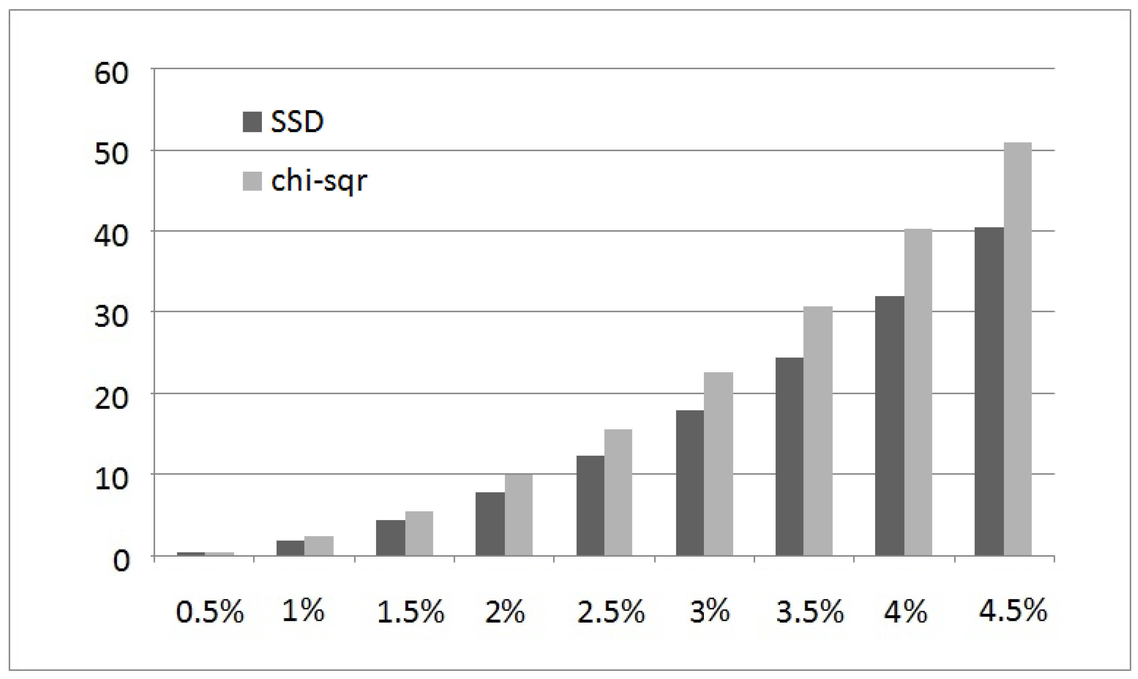
Figure 23 depicts resultant SSD and chi-square values in each example. The bar chart in
Figure 24 depicts the resultant SSD and chi-square values of the table.
Remarkably, the ratio of (chi-square)/(SSD) is steady at 1.26 across all deviations. In essence, what it means is that, at least in such particular variation style for digits 1 and 9, the chi-square statistic could be viewed as merely another scale measuring the same phenomenon SSD does, namely deviation from Benford, not offering any new or novel ideas. Let us prove this, utilizing the definition of ∆ as the absolute value of the fractional deviations from Benford, such as 0.005, 0.01, 0.015, 0.02, 0.025, 0.03, 0.035, 0.04, 0.045, namely ∆ = |(Observed − Theoretical)|:
Namely (3.32 + 21.85)/(20) or (25.17)/(20), so that 1.26 is the ratio of (chi-square)/(SSD), for all values of deviation ∆, regardless.
The constancy of the ratios can be easily generalized to wider deviations from Benford, spread among many more digits, so long as all deviations can be expressed as ± multiples of some minimum or basic deviation Δ, and that the structure of deviations stays fixed among the digits, where each digit is being either increased or reduced by a fixed multiple of Δ deviation, such as in the case of:
The above results pointing to a constant ratio of (chi-square)/(SSD) for all values of deviation ∆,in many typical cases of deviations (where fixed chosen digits are affected by the same proportional deviations) suggest that there is no need to be much concerned about aiding high digits over and above low digits ostensibly in order to compensate for their milder fluctuations as opposed to the typically more dramatic fluctuations of the low digits. And this is so since SSD and chi-square here are a simply distinct scale of measurements which rise and fall together in exact proportions. Admittedly, when distinct proportional deviations occur at totally distinct digits, SSD and chi-square differ substantially and in a much more profound way than merely in a scale sense, as the chi-square statistic emphasizes deviations in high digits and deemphasizes deviations in low digits.
Is it really necessary to support the small and weak (high digits), at the expense of the big and powerful (low digits)? Proponents of the idea could point to the misleading example of suspected drought somewhere in Central Africa where unreliable reports of prolonged lack of rain have reached the reservation office and the personnel at the hunting association. In order to verify this drought condition the weight of several wild lions are measured and found that indeed the average lion weight has been reduced by 10 kg. A parallel study shows that the average weight of wild monkeys there has also been reduced by 10 kg. Since typical weight of a lion is 190 kg, meaning that they have lost only 10/190 or merely 5% of their weight, then no proof of drought exists. But the study of monkeys does cause an alarm, since typical weight of the monkey species there is merely 30 kg, meaning that they have lost 10/30 or a whopping 33% of their weight; hence the proof of the existence of drought is decisive.
But in the context of Benford’s Law, the digit deviations perspective is different, For example, a 3% transfer between the proportions of digits 8 and 9 does not seem more dramatic or substantial than, say, a 3% transfer between the proportions of digits 1 and 2.
The other highly significant difference between the chi-square statistic and the SSD measure is the involvement of the data size N in the construction of the chi-square statistic as a multiplicative factor. The SSD measure on the other hand is totally indifferent to the data size N.
Certainly, for a proper comparison measure with the Benford proportions, the term N should be strictly avoided, since it has no bearing whatsoever on the concept of “distance” from the Benford proportions in any sense; and any inclusion of the term N in the definition of the measure-either as a multiplicative factor or as a divisional factor-would indeed distort its meaning.
It should be acknowledged that the 1% or the 5% threshold probabilities values for the chi-square statistic are as arbitrary as any subjective threshold values constructed for the SSD. Indeed those SSD thresholds are arrived via extensive empirical studies of honest and naturally occurring real-life data, so they come with some solid foundations. As an example of the arbitrariness of these 1% and 5% values in the context of the chi-square test; if the researcher (who is dead set on declaring his/her set of numbers as Benford no matter what) disappointedly obtains 16.3 value for the chi-square statistic for the 1st digits of his/her data (which is below 5%), they can still declare 3% tolerance limit level and let it pass as Benford. And if they obtain 20.4 value for chi-square statistic (which is below 1%), they can then unfairly move the goalpost (post analysis) to 0.5% tolerance limit level, and thus be able supposedly to present their data as Benford. Surely the classic 1% and 5% thresholds so often used in statistical inference seem like nice, round, and whole numbers, yet they are still arbitrary!
Surely, there are infinitely many alternative definitions to SSD which could measure the distance to Benford from the digital configuration of a given data set—without involving the data size N. A famous one is the Mean Absolute Deviations or MAD, defined as:
This author chose the usage of SSD over MAD for two reasons. The first reason is that MAD numbers are typically very small fractional values which are difficult to internalize intuitively and are especially challenging in terms of memorizing the empirical or subjective threshold/cutoff values. The SSD measure on the other hand yields typically larger values between, say, 1 and 50 approximately and thus it is easier to work with and to memorize. The second reason is that the absolute value is difficult to work with mathematically, while squares are much easier in this regard, hence any future researcher, mathematician, or statistician, who might wish to derive new results or attempt to build some statistical framework of compliance, would probably find the squares in the SSD definition more suitable for mathematical manipulations than working with the cumbersome absolute value involved in the MAD definition. Indeed, such was the course of events that took place in the field of Linear Regression Analysis involving the Sum of Squares Total, Sum of Squares Regression, and Sum of Squares Error (SST, SSR, SSE) definitions, and which proved immensely successful and useful.
Let us demonstrate some alternative definitions to SSD and MAD, all properly signifying a measure of distance from Benford just as well:
The definitions of SSD and MAD appear the most simplistic, straightforward, and natural ones, except for their arbitrary scale/factor involved.
Obviously, the chosen subjective cutoff point or threshold value separating compliance from noncompliance depends on the definition of distance applied. A recent article by Cerqueti and Maggi utilizes an innovative method of varying the shape parameter of the Lognormal Distribution in order to establish a comparison between the threshold values of SSD and MAD as provided by their inventors. See [
9] for details of this study.
This author thrived to create threshold/cutoff values for his SSD measure of distance via extensive empirical examinations of real-life and abstract mathematically-driven data sets. These rough guidelines however were subjectively arrived at, albeit with outmost effort to make them as reasonable as humanly possible. The table in
Figure 25 provides these threshold values.
Increasingly, scholars apply both SSD as well as MAD in their Benford’s Law research, such as in [
10,
11,
12].
13. Testing the Lognormal via the Chi-Square Statistic
N Monte Carlo computer simulations are performed for the Lognormal distribution, with location parameter 11.0 and shape parameter 2.0. Thus, N effectively denotes the data size.
We record the 1st digits of these N truly independent simulations. Surely, each simulated value has no dependency or correlation with any other simulated value.
We then calculate resultant SSD and resultant chi-square statistic. This is called a “procedure”.
We repeat this simulation procedure 10 times in order to obtain a somewhat more robust and stable singular average value of 10 such SSD and chi-square values. A whole set of 10 such procedures and its associated SSD average and chi-square average is called a “scheme”.
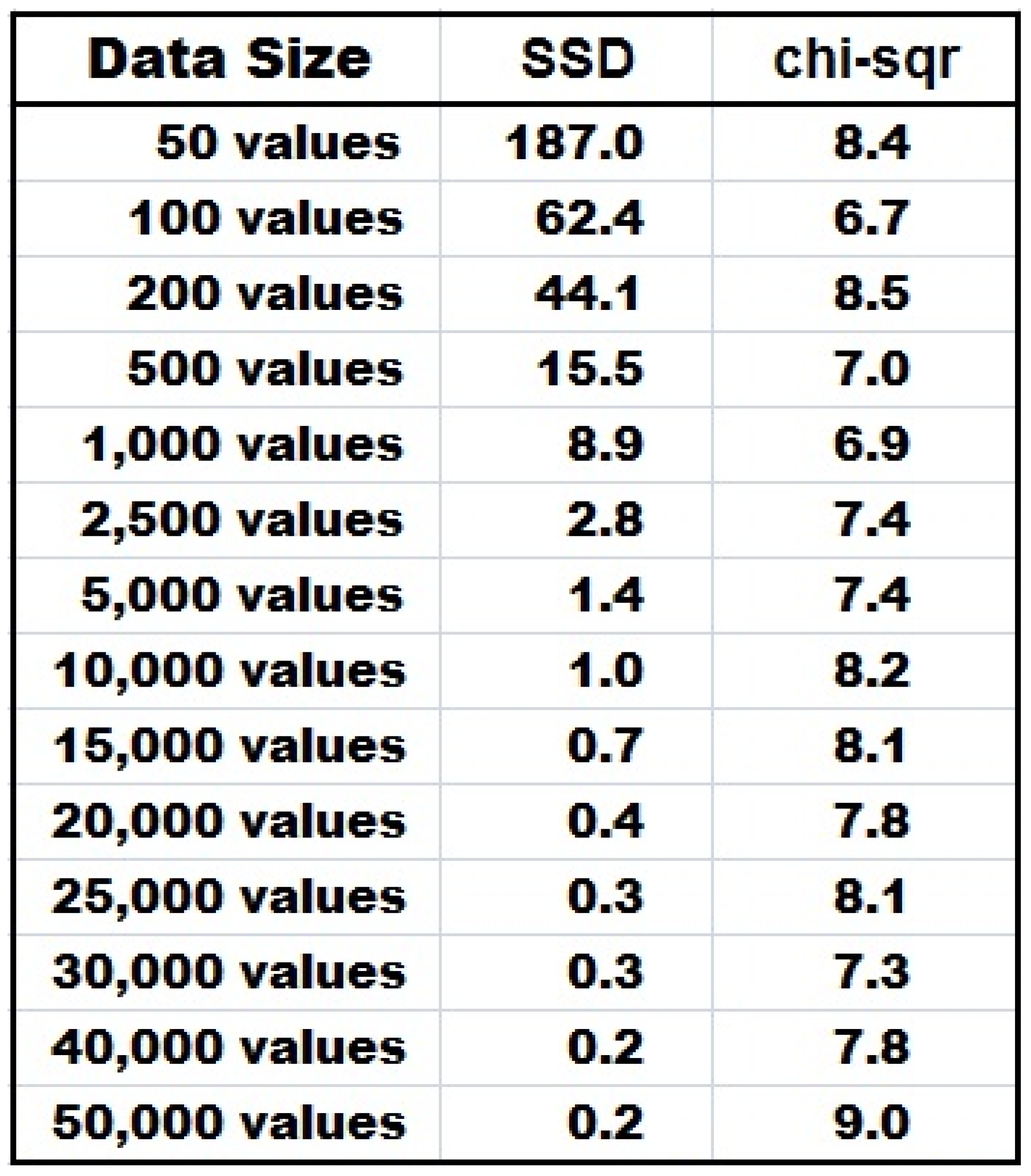
In total, we use 14 distinct values for N, from the lowest value of 50, to the highest value of 50,000. For each N we perform a scheme and obtain its SSD average and chi-square average.
The results of these 14 Monte Carlo schemes are given in the table of
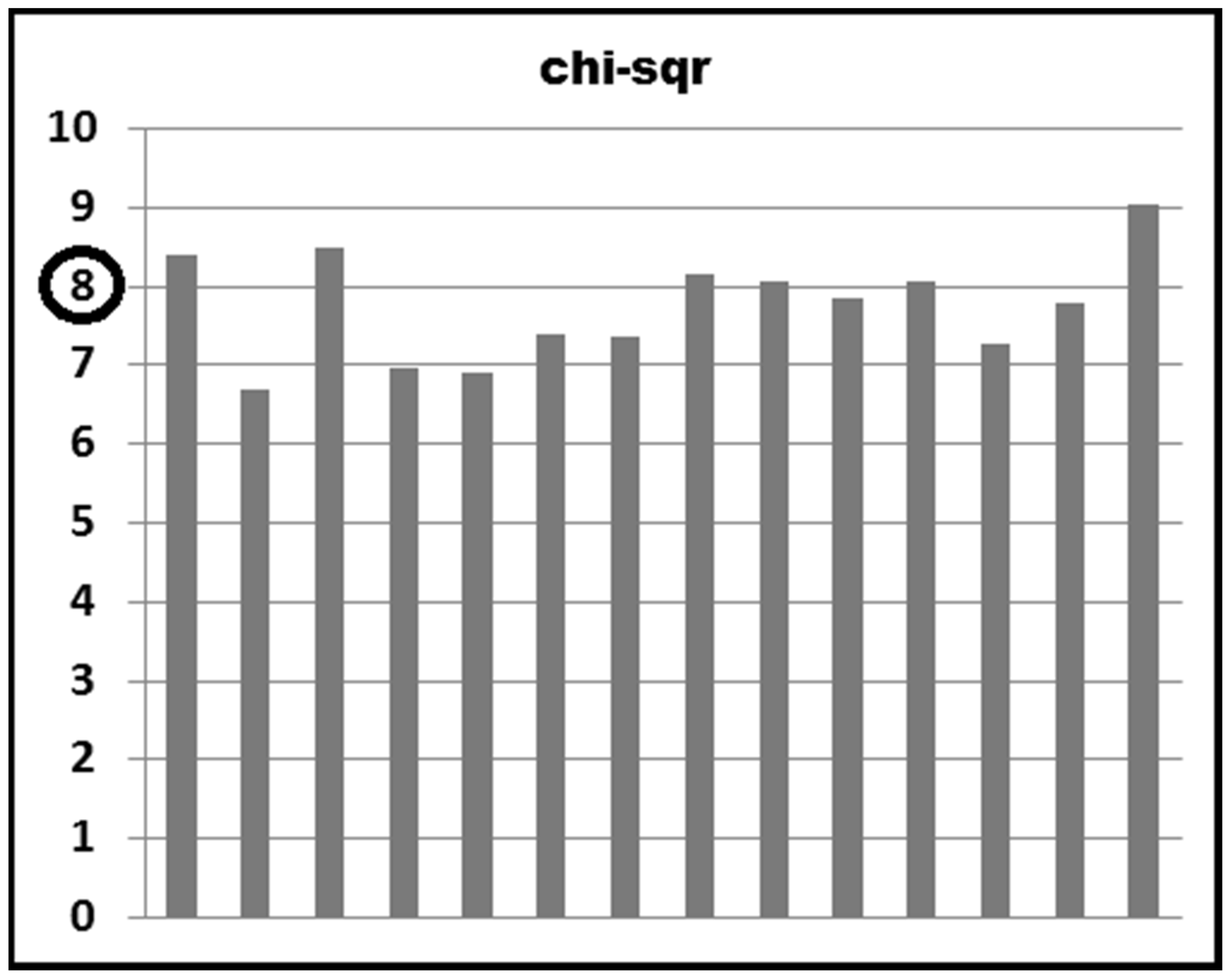
Figure 26 and its associated bar chart of
Figure 27.
Everything makes sense!
The expected value of chi-square with 8 degrees of freedom is 8!
As N advances from 50 to 50,000, the fit to Benford gets better and better, but since we are obliged to multiply the sum of the nine deviations by N to obtain the chi-square statistic, the reduction in deviations is being canceled out and offset (almost exactly) by the increase in the value of N, so that we always get about an average value of 8 for the chi-square statistic.
Each simulation value of the Lognormal is truly independent of all its brothers and sisters simulations! For example, for N = 50,000 simulations, we truly and honestly have independent random selection processes from the Lognormal Benford Universe 50,000 times! It is noted that 99% of that Benford Universe of the Lognormal(11, 2) falls on the interval between 347 and 10,341,325, and that this range of possibilities is uncountably infinite. Admittedly, the random number generator within any computer system cannot generate infinite possibilities of random values, yet, the scope of the computer’s random number is truly huge even though it is finite.
Conclusion:
It stands to reason to calculate and present the chi-square statistic as a decisive indication of compliance or non-compliance with Benford for a batch of values derived (independently) from the Lognormal distribution (or for any random distribution whatsoever for that matter!)
14. Testing the Fibonacci Series via the Chi-Square Statistic
We select N values from the Fibonacci Series, beginning from 1, 1, 2, 3, 5, 8, 13, and so forth.
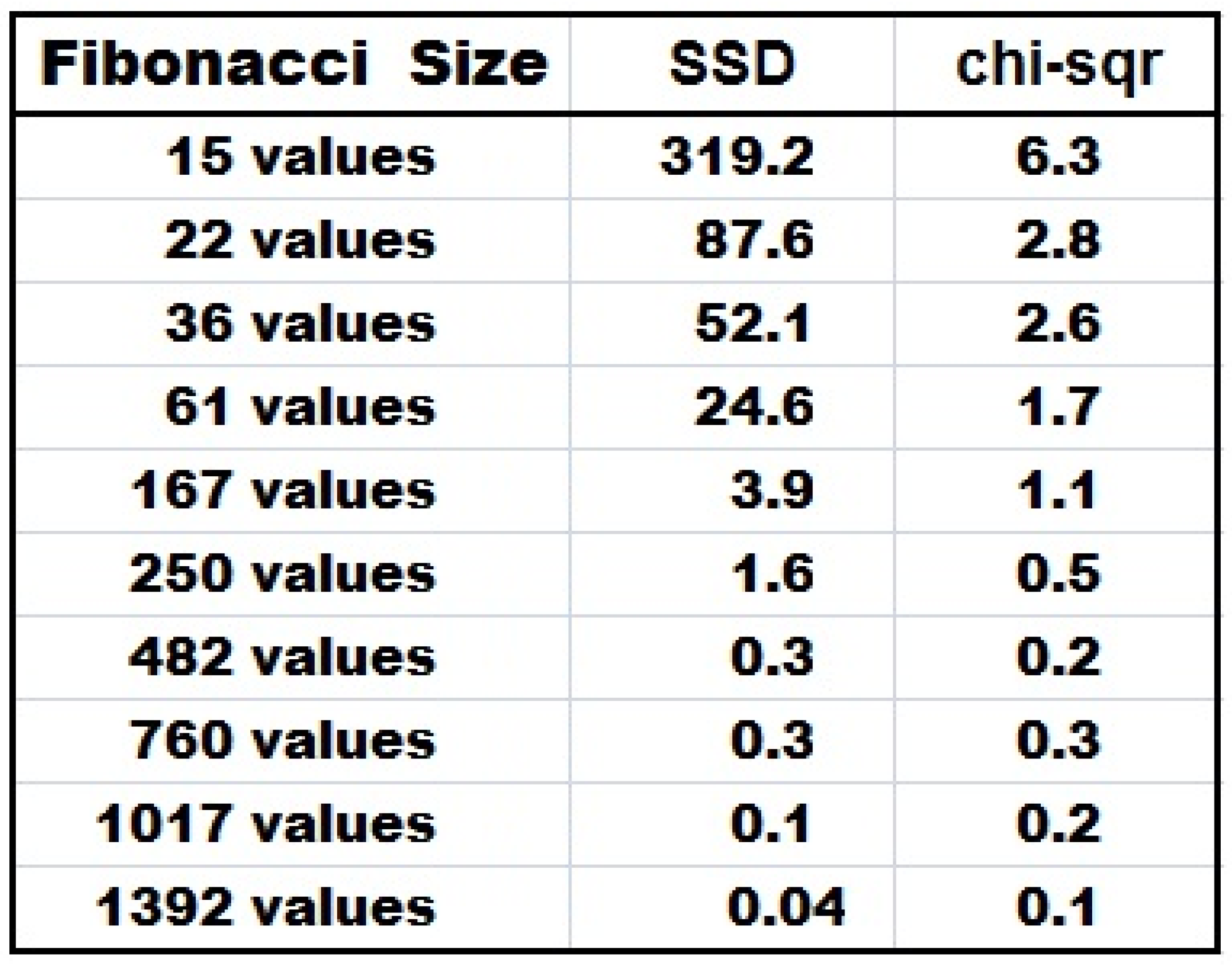
In total we choose 10 distinct N sizes, from the small size 15, to the biggest size 1392, yielding 10 distinct Fibonacci Series of distinct sizes, all beginning from 1, 1, 2, 3, 5, 8, 13, and so forth.
We record the 1st digits of these distinct Fibonacci Series of distinct N sizes.
Then we calculate resultant SSD and resultant chi-square statistic for each N size.
Nothing makes sense!
Each value within a given Fibonacci Series of fixed size N is very much dependent on its adjacent values, since all values within the series are ordered and totally predictable! The values here are not found via some independent and random selection processes from some imaginary Benford Universe of data-one value at a time!
The sequence 1, 1, 2, 3, 5, 8, 13, and so forth, is decisively deterministic and exact.
It is not some random process deserving of the chi-square statistical procedure.
Hence it would be erroneous to blindly apply the chi-square test in this case of the Fibonacci series, yet, it is mistakenly presented as some sort of a valid measure of deviation or compliance with Benford’s Law! The fact that the application of the chi-square test indeed correctly certifies the Fibonacci series with compliance with Benford’s Law does not absolve it in any way of misleading us about its methodology and its relevance.
There could never be a discussion here of the “probability” of obtaining a chi-square statistic over this or that threshold value, or of any supposed confidence intervals, and so forth.
The value of the chi-square statistic itself is immediately determined and known in advance once we decide on the value of the series size N, and it does not vary in any random way.
Conclusion:
Any given Fibonacci Series of a fixed size possesses a certain fixed and deterministic first digit distribution, and it does not make any sense to calculate and present a ‘chi-square statistic’ as some sort of Benford measure, and especially not as something masquerading as Benford compliance measure based on probability calculations.
15. Testing Partial US Population Data Sets via the Chi-Square Statistic
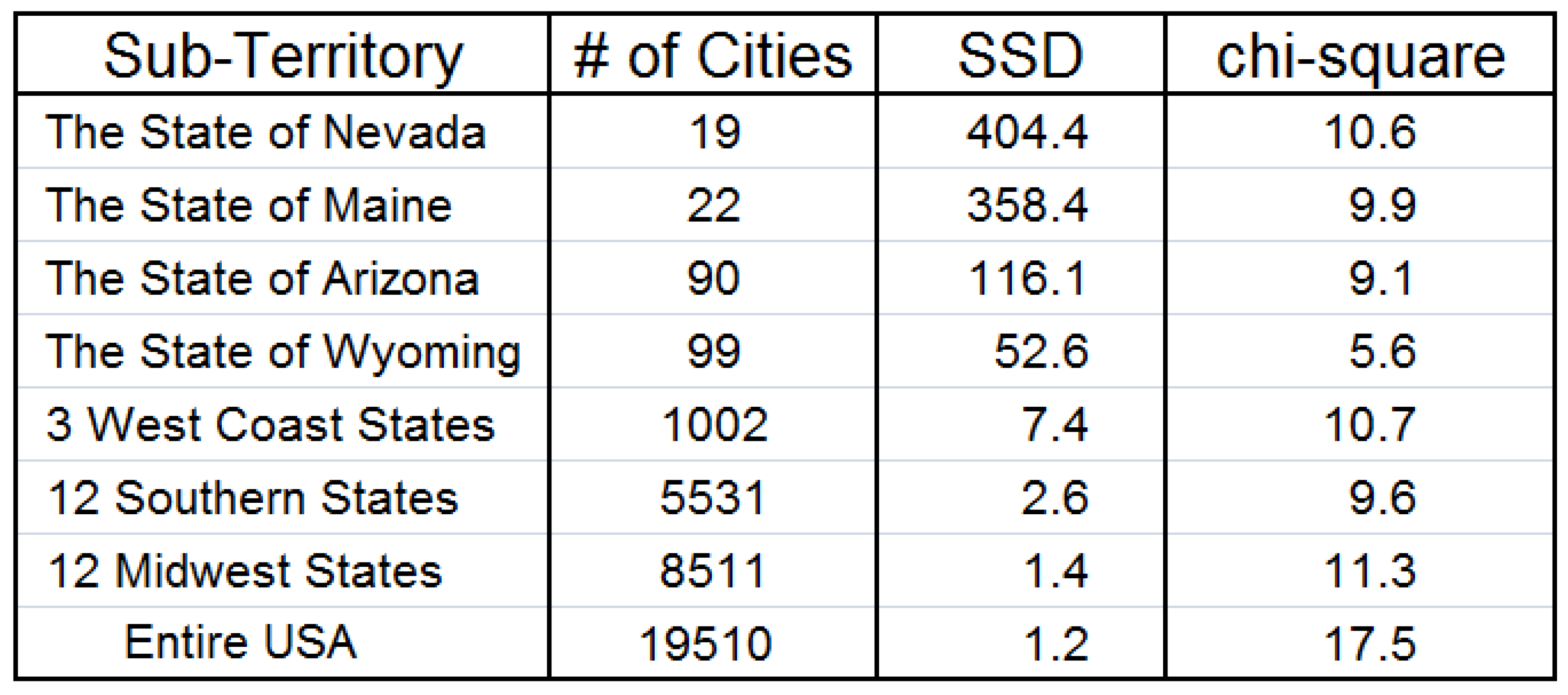
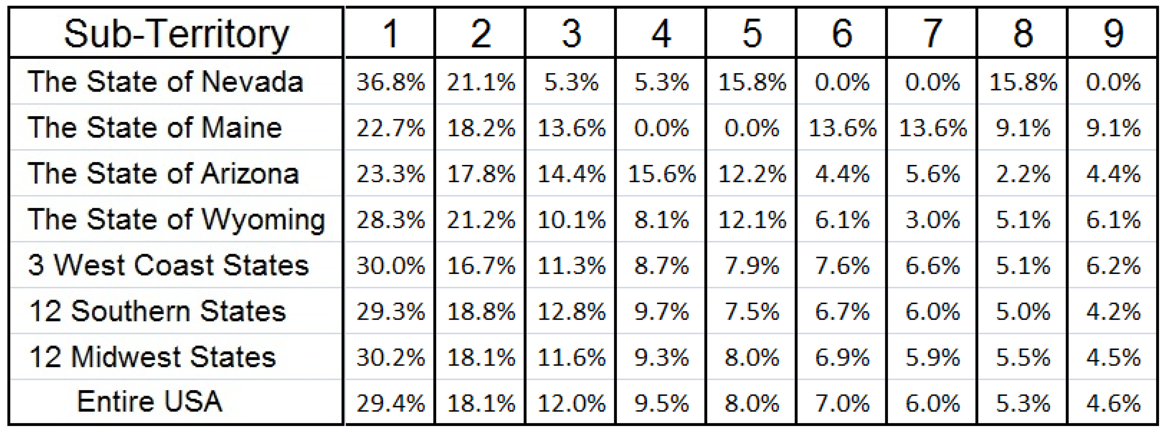
We select particular sub-territories from the USA regarding its 2009 population data, and we order them in such a way as to steadily increase the size of these sub-data-sets, namely, we organize them with increasing number of city centers. In total 7 mini data sets representing 7 sub-territories are extracted from the original available USA data set, namely, the population data of 4 particular states, as well as 3 groups of states in the West, South, and Midwest.
Then resultant SSD and chi-square statistic are calculated and displayed for each sub-territory.
The table in
Figure 29 depicts the digital summary results. The table in
Figure 30 details the 1st digit distributions.
Results seem contradictory!
For small-size territories, such as Nevada, Maine, Arizona, and Wyoming, deviations from Log(1 + 1/d) proportions are quite high, but since N is relatively small, the chi-square statistic is low enough to point to “compliance” with the law. As the size of the territories increases over 1000 cities, the value of N within the expression of the chi-square statistic becomes much larger, yet, since at the same time deviations from Log(1 + 1/d) proportions become much smaller, the chi-square statistic remains approximately the same and continues to declare “compliance”.
In other words, as the size of the territories increases steadily, it induces a tug-of-war between the reduction in deviations from Log(1 + 1/d) proportions, and the increase in the value of N, and this “conflict” yields nearly a draw or a tie regarding resultant value of the chi-square statistic, as both factors exert nearly equal and balanced influence on it. Yet, eventually, as N reaches 19,510 city centers for the entire USA data without any corresponding further drastic reduction in deviations from the Log(1 + 1/d) proportions, chi-square finally gives in from the pressure of the high value of N, as it attains the high value of 17.5, standing well above the cutoff point of 15.5 for 5% confidence interval, and so the test declares the entire US data set to be non-Benford.
The striking contrast between the conclusions of the chi-square test regarding the 12 Midwest states and the entire USA data set is quite odd! A quick glance of the actual digit distributions in
Figure 30 for these two sets of data reveals a great deal of similarities, yet the lower N value of 8511 for the Midwest as compared with the high N value of 19,510 for the entire USA, causes the chi-square test to arrive at two opposing conclusions for these similarly distributed (digit-wise) sets of data.
Conclusion:
Are we to believe that we are truly following the proper mathematical statistics model here? Are we to believe that it is proper for the chi-square test to enthusiastically endorse these small states and to declare them as Benford, even though their digits distributions deviate a great deal from the Log(1 + 1/d) proportions, and also to endorse some grouping of states as Benford as well, while refusing to acknowledge the entire set of the USA data as Benford, even though it is the parent population data from which those smaller sub-territories are concocted from, and even though the entire USA digit distribution is the one set of data closest to the Log(1 + 1/d) ideal proportions as seen from its exceedingly low SSD value of 1.2?
Let us recapitulate; the chi-square test declares the whole as non-Benford, while at the same time it certifies parts of it as Benford!?
The reason for the “odd behavior” of the chi-square test here is that data points (cities) are not independently “selected” from some imagined much larger (global) universe of population data, one city at a time, as in a proper random sampling process. Admittedly the population of each city is indeed a random and probabilistic number, and there is nothing deterministic and predictable about it, yet the populations of (nearby) cities are not independent of each other, and there was never any actual sampling process involved here, one city at a time.
16. The Nature of Hypothetical Real-Life-Like Revenue Data
To the naïve, the calculation and presentation of the chi-square statistic for real-life data sets may appear as standing (conceptually) somewhere half way between the two extreme poles of the purely random Lognormal case and the purely deterministic Fibonacci case, yet in reality this is not so due to dependency between data points, and because of the fact that, almost always, data is not obtained via some purely random process which selects numbers one value at a time from some larger Benford universe of numbers.
Indeed, real-life data sets such as census data, election data, population data, accounting data, physical, astronomical, and geological data, and so forth, are such that the values are often dependent on each other. Data points within a given data set often rise and fall together or separately, namely being positively or negatively correlated to one another. Many (but not all) individual data points within a given real-life data set certainly relate to and depend on other data points in many ways.
The table shown in
Figure 31 depicts several hypothetical sale amounts at a small bakery, selling bread loafs, cheese cakes, and cookies. Clearly, a large sale of 5 bread loafs for the office of IT-EDU company would imply that no additional such sales would occur during the rest of the day as everybody there is already full and that nobody will be hungry anymore soon, thus demand there for bread is zero. In addition, knowledge about the high quality of the delicious products baked there is spread via rumors especially after one successful sale in one office, and then leads to another sale in another office, such as the sale of 11 bread loafs at CCNET office after employees there were informed by IT-EDU personnel about the high quality of the baked items for sale.
17. The Nature of Hypothetical Real-Life-Like Population Data
As another example, the USA population in 2009 contains 19,509 cities, towns, and villages.
The smallest value is 1, namely a single habitant in one officially-registered village. The biggest value is 8,391,881 for New York City. Even though this data set is very close to Benford, the chi-square test fails to certify the data as Benford.
Let us critically and open-mindedly examine a tiny sample collected from that vast US data set, and focused only on a few cities and towns in the state of New Mexico as seen in the table of
Figure 32.
Let us further focus on the city of Santa Fe with its population of 67,947. This value point within the USA data set of 19,509 cities did not arise from a process of picking blindly from some imaginary and much larger global Benford universe of population numbers. Rather, this value is the result of 430 years of long and complex history involving immigration and migration, within the state of New Mexico, as well between it and the entire USA, Mexico, and some European countries. This value also relates to deaths and births, accidents, illnesses, businesses, jobs, and random romantic involvements during all those years. In a very small part, the final value of 67,947 inhabitants relates to a single Mexican farmer from Guadalajara and his small family of 5 children and a wife, moving north in 1627 in search of more fertile and cooler lands. It also relates to the (imagined) 1719 Cholera Epidemic, which broke out in the area and which killed around 25% of the population. This population value of 67,947 also strongly relates to the secretive Manhattan Project established in nearby Los Alamos which was most active during the years 1942 to 1946, and which had directly and indirectly boosted considerably the population of Santa Fe.
The first digit 6 of Santa Fe population value 67,947 had not been simply picked up randomly from some multinomial distribution; rather, the complex numerical value of 67,947 had finally arrived at after 430 years of very long and complex history. The town of Ruidoso on the other hand had a totally distinct history and manner of growing. To recapitulate; this Santa Fe value of 67,947 inhabitants was not obtained via some easy, smooth, and effortless single random selection from some large Benford pool or enormous box of numbers in a sampling process which took merely 5 s to accomplish.
State residents frequently move their residences from one town to another city, say a family moving from Albuquerque to Santa Fe, or from Rio Rancho to Tularosa, and from Rio Rancho to Tijeras, and so forth, hence the values are certainly not independent from each other.
Surely, the little far away town of Lansdale in Pennsylvania with the modest population of 16,675 is nearly independent of, say, the town of Tatum in New Mexico with its population of 798 inhabitants, as there exist probably no immigration or any connection almost between these two far away towns. On the other hand, nearby cities and towns in the same state, or even in neighboring states are highly dependent on each other, and so the chi-square approach is wholly inappropriate. All this demonstrates very clearly why the chi-square test approach is totally inappropriate and absolutely meaningless for population data sets in general.
18. Conclusions
The application of the chi-square test in the context of compliance with Benford’s Law is almost never justified for nearly all data types, as the mathematical statistical basis is scrutinized and its irrelevance to the data set on hand is revealed.
The chi-square test is applicable to Benford’s Law if and only if each data point on hand (our sample, namely our data set under consideration) has been randomly selected from a much larger or infinite universe of parental data, while that process was carried out in such a way as to ensure the independence of the selection of each data point from the selections of all the other data points. Indeed, frequently, that parental universe of numbers might not even exist, except in the feverish and highly imaginative mind of the naïve statistician.
Another major blow to the whole concept of applying the chi-square test is revealed when indeed the data set on hand is confidently known to be have been truly obtained randomly and selected one value at a time from a universe of parental data with independence of each data point. In this case, the parental universe is either confidently known to be Benford, or its Benford status is still unknown to the researcher.
If the parental universe is confidently known to be Benford, then the chi-square test is not needed at all as it serves no function whatsoever. For example, obtaining only around 10 values could not possibly lead to anything near the Benford configuration, no matter how lucky one gets. Obtaining around 50 values would probably lead to a configuration similar to Benford but not close enough. On the other hand, gathering tens of thousands of values would guarantee a near perfect Benford configuration. The chi-square statistic itself here would most likely always be well below the 5% threshold value of 15.5, since our parental universe is indeed Benford and since we truly select one value at a time randomly and independently. Most likely the chi-square statistic would almost always be quite near the expected value of 8 (as in 8 degrees of freedom chi-square distribution for the 1st digits).
If the Benford status of the parental universe is still unknown to the researcher, then the chi-square statistic should be very high—if parental universe is non-Benford and data size N is large, or it should be much lower near 8—if parental universe is Benford, or it should be somewhere in between approximately—if parental universe is only partially Benford and data size N is not too small. Hence, in this case, it should be acknowledged that the focus and conclusion of the chi-square test is all about the reasonableness of the entire random selection process and the Benford status of the parental universe of numbers, and not solely about the data set on hand! The research question of the chi-square test here is actually stated as follows: “Is the parental universe of numbers truly Benford and the selection process probable?” Or alternatively: “Is the probability of obtaining the digital structure of our data set with its associated size N reasonable enough, given that the parental universe of numbers is truly Benford?” The focus is not about the closeness of the digital structure of our data to the Benford’s structure, nor about its size N, but rather whether the probability of obtaining our sample from the parental population of numbers was fairly reasonable and not too rare—assuming that the parental universe of numbers is truly Benford. Rareness, such as when the chi-square test yields p value less than 1% simply implies that our assumption about the parental universe of numbers being Benford was incorrect. Arithmetically, this p value (the chi-square statistic in essence) is obtained via the combination (the confluence) of the deviation of our data from Benford as well as the sample size N. Yet, the chi-square test says nothing uniquely about the digital structure of our sample on hand (without considering its size in this context). The chi-square test is simply not interested in examining exclusively the closeness of our data to the Benford configuration, but rather whether or not sampling was not too rare probabilistic-wise under the assumption that the parental universe is Benford.
The table in
Figure 33 contains a summary of possible occurrences and scenarios with regards to 1st digits whenever the researcher confidently knows that data has been obtained truly randomly from a parental universe of data, and that all data points have been selected independently of each other.
The table in
Figure 33 evidently demonstrates that knowledge about the small magnitude of the chi-square statistic does not help in determining the digital configuration of the given data set. On the other hand, a particularly big magnitude of the chi-square statistic decisively determines that the parental universe of numbers as well as the data set are definitely not Benford.
The frequent complaints about the “excess power” (the first paradox) of the chi-square test, namely when data size N is very large and the chi-square test appears as if too strict, as well as the less frequent complaints about the “suppressed power” (the second paradox) of the chi-square test, namely when data size N is very small and the chi-square test suddenly appears to be very liberal and too permissive, are merely two mild manifestations of symptoms of some underlying serious disease, which is the application of the chi-square test for data which is not created via selections one data point at a time from some larger universe of numbers, independently. The goal of this article and its “medical approach” is not to temporarily and superficially suppress the symptoms of the patient, but rather to holistically, permanently, and thoroughly cure the patient once and for all.

