Robust Fitting of a Wrapped Normal Model to Multivariate Circular Data and Outlier Detection

Abstract

In this work, we deal with a robust fitting of a wrapped normal model to multivariate circular data. Robust estimation is supposed to mitigate the adverse effects of outliers on inference. Furthermore, the use of a proper robust method leads to the definition of effective outlier detection rules. Robust fitting is achieved by a suitable modification of a classification-expectation-maximization algorithm that has been developed to perform a maximum likelihood estimation of the parameters of a multivariate wrapped normal distribution. The modification concerns the use of complete-data estimating equations that involve a set of data dependent weights aimed to downweight the effect of possible outliers. Several robust techniques are considered to define weights. The finite sample behavior of the resulting proposed methods is investigated by some numerical studies and real data examples.

1. Introduction

Circular data arise commonly in many different fields such as earth sciences, meteorology, biology, physics, and protein bioinformatics. Examples are represented by the analysis of wind directions [1,2], animal movements [3], handwriting recognition [4], and people orientation [5]. The reader is advised to read the work in [6,7] to become familiar with the topic of circular data and find several stimulating examples and areas of application.

In this paper, we deal with the robust fitting of multivariate circular data, according to a wrapped normal model. Robust estimation is supposed to mitigate the adverse effects of outliers on estimation and inference. Outliers are unexpected anomalous values that exhibit a different pattern with respect to the rest of the data, as in the case of data orientated towards certain rare directions [3,8,9]. In circular data modeling, in the univariate case, the data can be represented as points on the circumference of the unit circle. The idea can be extended to the multivariate setting, where observations are supposed to lie on a $p-$dimensional torus, by revolving the unit circle in a $p-$dimensional manifold, with $p\ge 2$. Therefore, the main aspect of circular data is periodicity, that reflects in the boundedness of the sample space and often of the parametric space.

The purpose of robust estimation is twofold: On the one hand we aim to fit a model for the circular data at hand and on the other hand, an effective outlier detection rule can be derived from the robust estimation technique. The latter often gives very important insight into the data generation scheme and statistical analysis. Looking for outliers and investigating their source and nature could unveil unknown random mechanisms that are worth studying and may not have been considered otherwise. It is also important to keep in mind that outliers are model dependent, since they are defined with respect to the specified model. Then, an effective detection of outliers could be a strategy to improve the model [10]. We further remark that an outlier detection rule cannot be derived by a non-robust method that is sensitive to contamination in the data, such as maximum likelihood estimation.

There have been several attempts to deal with outliers in circular data analysis, mainly focused on the Von Mises distribution and univariate problems [2,11,12,13]. A first general attempt to develop a robust parametric technique in the multivariate case can be found in [9]: The authors focused on weighted likelihood estimation and considered outliers from a probabilistic point of view, as points that are unlikely to occur under the assumed model. A different approach, based on computing a local measure of outlyingness for a circular observation with respect to the distance from its k nearest neighbors, has been suggested in [14].

In this paper, we propose a novel robust estimation scheme. The key idea is that outlyingness is not measured directly on the torus as in [9] but only after unwrapping the multivariate circular data from the p-dimensional torus onto a hyperplane. This approach allows one to search for outliers based on their geometric distance from the robust fit. In other words, the main difference between the proposed technique and that discussed in [9] lies in the downweighting strategy: Here, weights are evaluated over the data unwrapped onto ${\mathbb{R}}^p$, whereas in [9], the weights are computed directly on the circular data over the torus and the fitted wrapped model.

In particular, we focus on the multivariate wrapped normal distribution, that, despite its apparent complexity, allows us to develop a general robust estimation algorithm. Alternative robust estimation techniques are considered, such as those stemming from M-estimation, weighted likelihood, and hard trimming. It is worth noting that to the extent of our knowledge, M-estimation and hard trimming procedures have never been considered in robust estimation for circular data, neither in univariate problems, nor in the multivariate case. In addition, the weighted likelihood approach adopted here differs from that employed in [9], according to the comments above.

The proposed robust estimation techniques also lead to outlier detection strategies based on formal rules and the fitted model, by paralleling the classical results under a multivariate Normal model [15]. It is also worth remarking that the methodology can be extended to the family of wrapped elliptically symmetric distributions.

The rest of the paper is structured as follows. In Section 2 we give some necessary background about the multivariate wrapped normal distribution and about the maximum likelihood estimation approach. This represents the starting point for the newly established robust algorithms that are introduced in Section 3. Outlier detection is discussed in Section 4. The finite sample behavior of the proposed methodology is investigated through some illustrative synthetic examples in Section 5, and numerical studies in Section 6. Real data analyses are discussed in Section 7. Concluding remarks finalize the paper in Section 8.

2. Fitting a Multivariate Wrapped Normal Model

The multivariate wrapped normal distribution is obtained by component-wise wrapping a p-variate normal distribution $\mathit{X}\sim N_p(\mathit{\mu },\mathsf{\Sigma })$ on a $p-$dimensional torus [16,17,18] according to $Y_d=X_d\mathrm{mod}2\pi$, $d=1,2,\dots ,p$. Formally, $\mathit{Y}=\mathit{X}\mathrm{mod}2\pi$ is multivariate wrapped normal and the modulus operator $\mathrm{mod}$ is performed component-wise. Then, we can write $\mathit{Y}\sim W{N}_p(\mathit{\mu },\mathsf{\Sigma })$.

The density function of $\mathit{Y}$ takes the form of an infinite sum over ${\mathbf{Z}}^p$, that is:

$${\varphi }_p^{\circ }(\mathit{y};\mathit{\mu },\mathsf{\Sigma })=\sum _{\mathit{j}\in {\mathbf{Z}}^p}{\varphi }_p(\mathit{y}+2\pi \mathit{j};\mathit{\mu },\mathsf{\Sigma }),$$

(1)

where ${\varphi }_p(·)$ denotes the density function of $\mathit{X}$. The support of $\mathit{Y}$ is bounded and given by ${[0,2\pi )}^p$. Without loss of generality, we let $\mu \in {[0,2\pi )}^p$ to ensure identifiability. The $p-$dimensional vector $\mathit{j}$ represents the wrapping coefficients vector, that is, it indicates how many times each component of the $p-$toroidal data point has been wrapped. Hence, if we observed the vector $\mathit{j}$, we would obtain the unwrapped (unobserved and hence not available) observation $\mathit{x}=\mathit{y}+2\pi \mathit{j}$.

Given a sample $({\mathit{y}}_1,{\mathit{y}}_2,\dots ,{\mathit{y}}_n)$, the log-likelihood function is given by:

$$\ell (\mathit{\mu },\mathsf{\Sigma })=\sum _{i=1}^{n}log{\varphi }_p^{\circ }({\mathit{y}}_i;\mathit{\mu },\mathsf{\Sigma }).$$

(2)

Direct maximization of the log-likelihood function in (2) appears unfeasible, since it involves an infinite sum over ${\mathbf{Z}}^p$. A first simplification stems from approximating the density function (1) with only a few terms [6], so that ${\mathbf{Z}}^p$ is replaced by the Cartesian product ${\mathcal{C}}_{\mathcal{J}}={\otimes }_{s=1}^p\mathcal{J}$ where $\mathcal{J}=(-J,-J+1,\dots ,0,\dots ,J-1,J)$ for some J providing a good approximation. Therefore, maximum likelihood estimation can be performed through the Expectation-Maximization (EM) or Classification-Expectation-Maximization (CEM) algorithm based on the (approximated) classification log-likelihood:

$${\ell }_c(\mathit{\mu },\mathsf{\Sigma })=\sum _{i=1}^n\sum _{\mathit{j}\in {\mathcal{C}}_{\mathcal{J}}}{v}_{i\mathit{j}}log{\varphi }_p({\mathit{y}}_i+2\pi \mathit{j};\mathit{\mu },\mathsf{\Sigma }),$$

(3)

where ${\mathit{v}}_{i\mathit{j}}=1$ or ${\mathit{v}}_{i\mathit{j}}=0$ according to whether ${\mathit{y}}_i$ has $\mathit{j}\in {\mathcal{C}}_{\mathcal{J}}$ as the wrapping coefficients vector.

The CEM algorithm reveals a particularly appealing way to perform maximum likelihood estimation both in terms of accuracy and computational time [8]. The CEM algorithm alternates between the CE step:

$$\begin{array}{cc}\hfill {\widehat{v}}_{i\mathit{j}}^{\left(s\right)}=& \frac{{\varphi }_p({\mathit{y}}_i+2\pi \mathit{j};{\mathit{\mu }}^{\left(s\right)},{\mathsf{\Sigma }}^{\left(s\right)})}{{\sum }_{\mathit{j}\in {\mathcal{C}}_{\mathcal{J}}}{\varphi }_p({\mathit{y}}_i+2\pi \mathit{j};{\mathit{\mu }}^{\left(s\right)},{\mathsf{\Sigma }}^{\left(s\right)})}\hfill \\ \hfill {\widehat{{\mathit{j}}_{\mathit{i}}}}^{\left(s\right)}=& {\mathrm{argmax}}_{\mathit{j}}{\widehat{v}}_{i\mathit{j}}^{\left(s\right)}\hfill \\ \hfill {\widehat{\mathit{x}}}_i^{\left(s\right)}=& {\mathit{y}}_i+2\pi {\widehat{{\mathit{j}}_i}}^{\left(s\right)}\hfill \end{array}$$

(4)

and the M-step:

$$\begin{array}{cc}\hfill {\widehat{\mathit{\mu }}}^{(s+1)}=& \frac{1}{n}\sum _{i=1}^n{\widehat{\mathit{x}}}_i^{\left(s\right)}\hfill \\ \hfill {\widehat{\mathsf{\Sigma }}}^{(s+1)}=& \frac{1}{n}\sum _{i=1}^n{\widehat{\mathit{x}}}_i^{\left(s\right)}{\left({\widehat{\mathit{x}}}_i^{\left(s\right)}\right)}^{\top }.\hfill \end{array}$$

(5)

If the wrapping coefficients were known, we would obtain that ${\mathit{x}}_i={\mathit{y}}_i+2\pi \mathit{j}$, $i=1,\dots ,n$, are realizations from a multivariate normal distribution. Notice that, under such circumstances, the estimation process in (5) resembles that concerning the parameters of a multivariate normal distribution. Then, the wrapping coefficients can be considered as latent variables and the observed circular data $\mathit{y}$ as being incomplete [8,19,20].

We stress that in each step, the algorithm allows us to deal with multivariate normal data ${\widehat{\mathit{x}}}_i$ obtained as the result of the CE-step in (4). Then, the M-step in (5) involves the computation of the classical maximum likelihood estimates of the parameters of a multivariate normal distribution.

3. A Robust CEM Algorithm

A robust CEM algorithm can be obtained by a suitable modification of the M-step (5), while leaving the CE-step unchanged. Indeed, robustness is achieved solving a different set of complete-data estimating equations given by:

$$\left\{\begin{array}{c}\sum _{i=1}^n{\psi }_{\mu }({\widehat{\mathit{x}}}_i;\mathit{\mu },\mathsf{\Sigma })=0\hfill \\ \sum _{i=1}^n{\psi }_{\mathsf{\Sigma }}({\widehat{\mathit{x}}}_i;\mathit{\mu },\mathsf{\Sigma })=0\hfill \end{array}\right.$$

(6)

where the estimating equation $\psi ={({\psi }_{\mathit{\mu }},{\psi }_{\mathsf{\Sigma }})}^{\top }=\mathbf{0}$ is supposed to define a bounded influence and/or high breakdown point estimator of multivariate location and scatter [10,21,22]. The resulting algorithm is a special case of the general proposal developed in [23], which gives very general conditions for consistency and asymptotic normality of the estimator defined by the roots of (6). The main requirements are unbiasedness of the estimating equation, the existence of a positive definite variance-covariance matrix ${\mathrm{E}}_{\mathit{\mu },\mathsf{\Sigma }}\left(\psi {\psi }^{\top }\right)$, and of a negative definite partial derivatives matrix ${\mathrm{E}}_{\mathit{\mu },\mathsf{\Sigma }}\left(\frac{\partial \psi }{\partial (\mathit{\mu },\mathsf{\Sigma })}\right)$.

In this paper, we suggest a very general strategy that parallels the classical approaches to robust estimation of multivariate location and scatter under the common multivariate normal assumption, that can be easily extended to the more general setting of elliptical symmetric distributions. In this respect, it is possible to use estimating equations as in (6) that satisfy the above requirements. In particular, we will consider estimating equations characterized by a set of data dependent weights that are meant to downweight those data points that exhibit large Mahalanobis distances from the robust fit. The Mahalanobis distance is defined over the complete unwrapped data as:

$$d=d(\widehat{\mathit{x}};\mathit{\mu },\mathsf{\Sigma })={\left[{(\widehat{\mathit{x}}-\mathit{\mu })}^{\top }{\mathsf{\Sigma }}^{-1}(\widehat{\mathit{x}}-\mathit{\mu })\right]}^{1/2}$$

and it is used to assess outlyingness. In the following, we illustrate some well-established techniques for a robust estimation of multivariate location and scatter that define estimating equations as in (5) to be used in the M-step.

3.1. M-Estimation

The M-step can be modified in order to perform M-estimation as follows:

$$\begin{array}{ccc}\hfill {\widehat{\mathit{\mu }}}_M^{(s+1)}& =& \frac{{\sum }_{i=1}^n{w}_i^{\left(s\right)}{\widehat{\mathit{x}}}_i^{\left(s\right)}}{{\sum }_{i=1}^n{w}_i^{\left(s\right)}}\hfill \\ \hfill {\widehat{\mathsf{\Sigma }}}_M^{(s+1)}& =& \frac{{\sum }_{i=1}^n{w}_i^{\left(s\right)}{\widehat{\mathit{x}}}_i^{\left(s\right)}{\left({\widehat{\mathit{x}}}_i^{\left(s\right)}\right)}^{\top }}{{\sum }_{i=1}^n{w}_i^{\left(s\right)}}\hfill \end{array}$$

(7)

with:

$$w_i^{\left(s\right)}=w_i({\widehat{d}}_i^{\left(s\right)})=w(d({\widehat{\mathit{x}}}_i^{\left(s\right)};{\widehat{\mathit{\mu }}}_M^{\left(s\right)},{\widehat{\mathsf{\Sigma }}}_M^{\left(s\right)}))$$

for a certain weight function $w(·)$. The weights are supposed to be close to zero for those data points exhibiting large distances from the robust fit. Well-known weight functions involved in M-type estimation are the classical Huber $w_H\left(t\right)=min(1,c/|t\left|\right)$ and Tukey $w_T\left(t\right)={[1-{(t/c)}^2]}^2\mathrm{I}\left(\right|t|\le c)$. The constant c regulates the trade-off between robustness and efficiency.

3.2. S-Estimation

In S-estimation, the objective is to minimize a measure of distances’ dispersion. Let $\mathsf{\Sigma }=\sigma \mathsf{\Gamma }$, where $\sigma$ denotes the size and $\mathsf{\Gamma }$, with $\left|\mathsf{\Gamma }\right|=1$, the shape of the variance-covariance matrix. Then, in the M-step one could update $(\mathit{\mu },\mathsf{\Gamma })$, minimizing some robust measure of scale of the squared distances, that is:

$$({\widehat{\mathit{\mu }}}_S^{(s+1)},{\widehat{\mathsf{\Gamma }}}_S^{(s+1)})=\mathrm{argmin}\widehat{\sigma }\left(d^2({\widehat{\mathit{x}}}_i^{\left(s\right)};\mathit{\mu },\mathsf{\Gamma })\right)$$

with $\mathsf{\Gamma }={\mathsf{\Sigma }\left|\mathsf{\Sigma }\right|}^{-\frac{1}{p}}$ and $\widehat{\sigma }$ is an M-scale estimate that satisfies:

$$\frac{1}{n}\sum _{i=1}^n{\rho }_{c_1}\left(\frac{d^2({\widehat{\mathit{x}}}_i^{\left(s\right)};\mathit{\mu },\mathsf{\Gamma })}{\widehat{\sigma }}\right)=K,0<K<sup{\rho }_c$$

where ${\rho }_c(·)$ is the Tukey bisquare function,

$${\rho }_c\left(t\right)=\left\{\begin{array}{cc}\frac{t^2}{2}-\frac{t^4}{2c^2}+\frac{t^6}{6c^4}\hfill & \mathrm{if}\left|t\right|\le c\hfill \\ \frac{c^2}{6}\hfill & \mathrm{if}\left|t\right|>c\hfill \end{array}\right.$$

with associated estimating function ${\psi }_T\left(t\right)=t{w}_T\left(t\right)$. It can be shown that the solution to the minimization problem satisfies M estimating equations [24]. The S-estimate for $\mathsf{\Sigma }$ is updated as ${\widehat{\mathsf{\Sigma }}}_S^{(s+1)}=\widehat{\sigma }{\widehat{\mathsf{\Gamma }}}_S^{(s+1)}$. The consistency factor $c_1$ determines the robustness-efficiency trade-off of the estimator. The reader is pointed to [25] for details about its selection.

3.3. MM-Estimation

S-estimation can be improved in terms of efficiency if the consistency factor used in the estimation of $(\mathit{\mu },\mathsf{\Gamma })$ is larger than that used in the computation of $\widehat{\sigma }$. Then, one could update $(\mathit{\mu },\mathsf{\Gamma })$ minimizing:

$$\frac{1}{n}\sum _{i=1}^n{\rho }_{c_2}\left(\frac{d^2({\widehat{\mathit{x}}}_i^{\left(s\right)};\mathit{\mu },\mathsf{\Gamma })}{\widehat{\sigma }}\right)$$

with $c_2>c_1$ and $\widehat{\sigma }=\widehat{\sigma }\left(d^2({\widehat{\mathit{x}}}_i^{\left(s\right)};\widehat{{\mathit{\mu }}_S^{(s+1)}},{\widehat{\mathsf{\Gamma }}}_S^{(s+1)})\right)$. The updated MM-estimate of $\mathsf{\Sigma }$ is ${\widehat{\mathsf{\Sigma }}}_{MM}^{(s+1)}=\widehat{\sigma }{\widehat{\mathsf{\Gamma }}}_{MM}^{(s+1)}$. A small value of $c_1$ in the first step leads to a high breakdown point, whereas a larger value $c_2$ in the second step corresponds to a larger efficiency [22,25,26].

3.4. Weighted Likelihood Estimation

The weighted likelihood estimating equations share the same structure of M-type estimating equations but with weights:

$$w\left(d\right)=\frac{{\left[A\left(\delta \right(d\left)\right)+1\right]}^{+}}{\delta \left(d\right)+1},$$

where $\delta \left(d\right)$ is the Pearson residual and $A\left(\delta \right)$ is the Residual Adjustment Function (RAF) [27,28,29,30,31], with ${[·]}^{+}$ denoting the positive part. Following [32], Pearson residuals can be computed comparing the vector of squared distances and their underlying ${\chi }_p^2$ distribution at the assumed multivariate normal model, as:

$$\delta \left(d_i\right)=\frac{{\widehat{f}}_n\left(d_i^2\right)}{m_{{\chi }_p^2}\left(d_i^2\right)}-1,i=1,2,\dots ,n,$$

where ${\widehat{f}}_n$ is an unbiased-at-the-boundary kernel density estimate based on the set of squared distances ${\widehat{d}}_i^2=d^2({\widehat{\mathit{x}}}_i^{\left(s\right)};{\widehat{\mathit{\mu }}}_W^{\left(s\right)},{\widehat{\mathsf{\Sigma }}}_W^{\left(s\right)})$ evaluated at the current parameters values obtained from weighted likelihood estimation and $m_{{\chi }_p^2}$ denotes the density function of a ${\chi }_p^2$ variate. The residual adjustment function can be derived from the class of power divergence measures, including maximum likelihood, Hellinger distance, Kullback–Leibler divergence, and Neyman’s Chi–Square, from the Symmetric Chi-Square divergence or the family of Generalized Kullback–Leibler divergences. It plays the same role as the Huber or Tukey function. The method requires the evaluation of a kernel density estimate in each step over the set $\left\{{\widehat{d}}_1^2,{\widehat{d}}_2^2,\dots ,{\widehat{d}}_n^2\right\}$. The kernel bandwidth allows control of the robustness-efficiency trade-off. Methods to obtain a kernel density estimate unbiased at the boundary have been discussed and compared in [32].

It is worth remarking that Pearson residuals could have been also computed in a different fashion through the evaluation of a multivariate non-parametric density estimate evaluated over the $\mathit{x}$ data or on the original torus data $\mathit{y}$. In the former case, a multivariate kernel density estimate should have been compared with a multivariate normal density. In the latter case, we need a suitable technique to obtain a multivariate kernel density estimate for torus data to be compared with the wrapped normal density. This approach has been developed in [9]. In a very general framework, the limitations related to the employment of multivariate kernels have been investigated in depth in [32]. The reader is also pointed to [33,34], who developed weighted likelihood-based EM and CEM algorithms in the framework of robust fitting of mixtures model.

3.5. Impartial Trimming Robust Estimation

In the M-step, we consider a 0–1 weight function, that is:

$$w_i=\left\{\begin{array}{cc}0\hfill & \mathrm{if}d({\widehat{\mathit{x}}}_i^{\left(s\right)};{\widehat{\mathit{\mu }}}^{\left(s\right)},{\widehat{\mathsf{\Sigma }}}^{\left(s\right)})>q\hfill \\ 1\hfill & \mathrm{if}d({\widehat{\mathit{x}}}_i^{\left(s\right)};{\widehat{\mathit{\mu }}}^{\left(s\right)},{\widehat{\mathsf{\Sigma }}}^{\left(s\right)})\le q\hfill \end{array}\right.$$

(8)

for a certain threshold q. This is also known as a hard trimming strategy. The cut-off q can be fixed in advance or determined in an adaptive fashion. Prominent examples are the Minimum Covariance Estimator (MCD, [35]) and the Forward Search [36], respectively. The computation of weights obeys an impartial trimming strategy, according to which, based on current parameters values in each step, distances are sorted in non-decreasing order, that is

$${\widehat{d}}_{\left(1\right)}^{\left(s\right)}\le {\widehat{d}}_{\left(2\right)}^{\left(s\right)}\le \dots \le {\widehat{d}}_{\left(n\right)}^{\left(s\right)},$$

and then, maximum likelihood estimates of location and scatter are computed over the non trimmed set. In other words, a null weight is assigned to those data points exhibiting the largest $\lfloor n\alpha \rfloor$ distances, where $\alpha \in [0,0.5]$ is the trimming level: In this case, we have $q={\widehat{d}}_{(n-\lfloor n\alpha \rfloor )}^{\left(s\right)}$. The variance-covariance estimate evaluated over the non trimmed set is commonly inflated to ensure consistency at the normal model by a factor $\gamma (p;\alpha )=\frac{1-\alpha }{F_{{\chi }_{p+2}^2}\left(q_{p,1-\alpha }\right)}$, where $F_{{\chi }_p^2}$ denotes the distribution function and $q_{p,1-\alpha }$ is the $(1-\alpha )$ level quantile of the ${\chi }_p^2$. A reweighting step can be also performed after convergence has been reached, with weights computed as in (8) on the final fitted distances with $q=q_{p,m}$ (common choices are $m=0.975,0.990$). The final estimates should be inflated as well, by the factor $\gamma (p;{\alpha }^{*})$, where now ${\alpha }^{*}$ is the rate of actual trimming in the reweighting step.

3.6. Initialization

A crucial issue in the development of EM and CEM algorithms is the choice of initial parameters values $({\mathit{\mu }}^{\left(0\right)},{\mathsf{\Sigma }}^{\left(0\right)})$. Moreover, to avoid dependence of the algorithm on the starting point and also to avoid being trapped in local or spurious solutions, it is suggested to run the algorithm from different initial values and then choose the solution that better satisfies some criterion. Here, starting values are obtained by subsampling. The mean vector $\mathit{\mu }$ is initialized with the circular sample mean. Initial diagonal elements of $\mathsf{\Sigma }$ are given by ${\mathsf{\Sigma }}_{rr}^{\left(0\right)}=-2log\left({\widehat{\rho }}_r\right)$, where ${\widehat{\rho }}_r$ is the sample mean resultant length; the off-diagonal elements of $\mathsf{\Sigma }$ are given by ${\mathsf{\Sigma }}_{rs}^{\left(0\right)}={\rho }_c({\mathit{y}}_r,{\mathit{y}}_s){\sigma }_{rr}^{\left(0\right)}{\sigma }_{ss}^{\left(0\right)}$ ($r\ne s$), where ${\rho }_c({\mathit{y}}_r,{\mathit{y}}_s)$ is the circular correlation coefficient, $r=1,2,\dots ,p$ and $s=1,2,\dots ,p$ [18]. The subsample size is expected to be as small as possible in order to increase the probability to get an outlier free initial subset but large enough to guarantee estimation of the unknown parameters. Several strategies may be adopted to select the best solution at convergence, depending on the robust methodology applied to update the parameters values. For instance, after MM-estimation, one could consider the solution leading to the smallest robust scale estimate among squared distances; when applying impartial trimming, one could consider the solution with the lowest determinant $|\widehat{\mathsf{\Sigma }}|$; the solution stemming from weighted likelihood estimating equations can be selected according to a minimum disparity criterion [32,33]; or minimizing the probability to observe a small Pearson residual over multivariate normal data ([9,32] and references therein).

3.7. Extension to Mixed-Type Data

It may happen that we are interested in the joint distribution of some toroidal and (multivariate) linear data. Let us denote the mixed-type data matrix as $(\mathit{Y},\mathbf{Z})$, where $\mathit{Y}$ is composed by $p_1$—dimensional circular data and $\mathbf{Z}$ by $p_2$—dimensional linear data. Such mixed-type data are commonly denoted as cylindrical [7]. Under the wrapped normal model $\mathit{Y}=\mathit{X}\mathrm{mod}2\pi$ in a component-wise fashion and $\mathit{X}$ has a multivariate normal distribution. If we knew the wrapping coefficients vectors, we could deal with a sample of size $p=p_1+p_2$ from a multivariate normal distribution. The unknown wrapping coefficients vectors are estimated in the CE-step (4), so that one can work with the complete data $(\widehat{{\mathit{x}}_{\mathit{i}}},{\mathit{z}}_{\mathit{i}})$ at each step.

4. Outlier Detection

Outlier detection is a task strongly connected to the problem of robust fitting, whose main aim is to identify those data showing anomalous patterns, or even no patterns at all, that deviate from model assumptions. For linear data, the classical approach to outlier detection relies on Mahalanobis distances [37,38]. Here, the same approach can be pursued on the inferred unwrapped data ${\widehat{\mathit{x}}}_i$ at convergence. Formally, an observation is flagged as an outlier when:

$$d^2({\widehat{\mathit{x}}}_i;\widehat{\mathit{\mu }},\widehat{\mathsf{\Sigma }})>q_{p;m},$$

(9)

where $m=0.950,0.975,0.990$ are common choices.

Outlier detection is the result of a testing strategy. For a fixed significance level, the process of outlier detection may result in type-I and type-II errors. In the former case, a genuine observation is wrongly flagged as an outlier (swamping), in the latter case, a true outlier is not identified (masking). Therefore, it is important to control both the level, provided by the rate of swamped genuine observations, and the power of the test, given by the rate of outliers correctly detected. The outlier detection rule can be improved by taking into account proper adjustments to correct for multiple testing and avoid excess of swamping [39].

5. Illustrative Synthetic Examples

In this Section, in order to illustrate the main aspects and benefits of the proposed robust estimation methodology, we consider a couple of examples with synthetic data. Here, the examples only concern bivariate torus data. The samples size is $n=500$ with $10\%$ contamination. We compare the results from the robust CEM described above in Section 3 and Maximum Likelihood Estimation (MLE) performed according to the classical CEM algorithm described in Section 2, with $J=3$. In particular, we consider MM-estimation with $50\%$ breakdown point and $95\%$ shape efficiency, the WLE with a symmetric chi-square RAF, and impartial trimming with $25\%$ trimming and reweighting based on the $0.975$-level quantile of the ${\chi }_2^2$ distribution. It is worth stressing that the breakdown point and the efficiency of the robust methods are tuned on the assumption of multivariate normality for the unwrapped data $\mathit{x}$. The robust CEM algorithm has been initialized from 20 different initial values evaluated over subsamples of size 10. Data and outliers have been plotted with different symbols and colors (available from the online version of the paper).

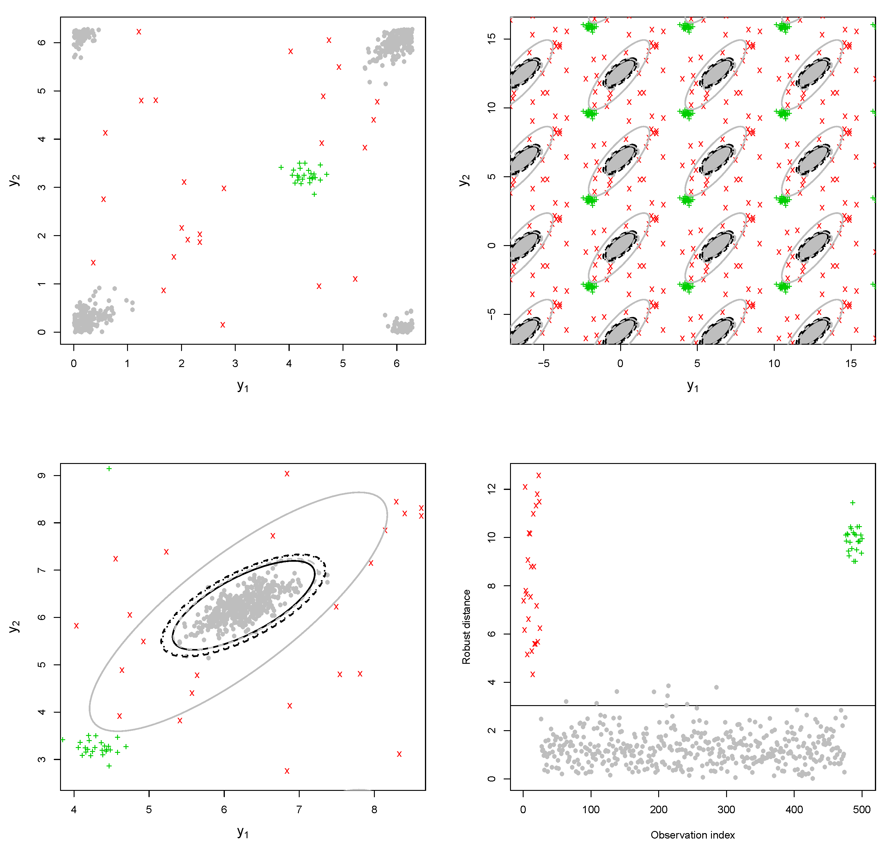
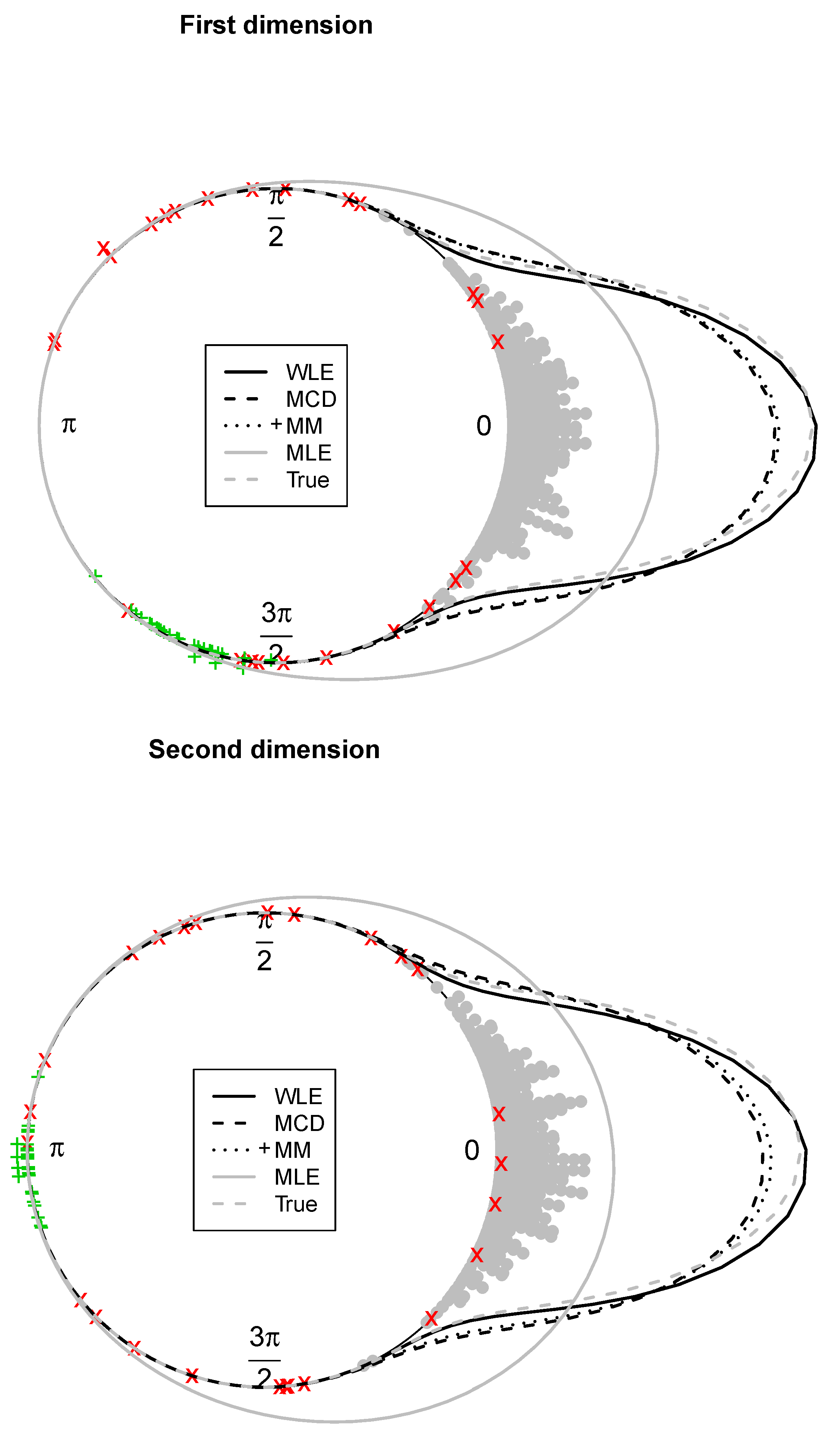
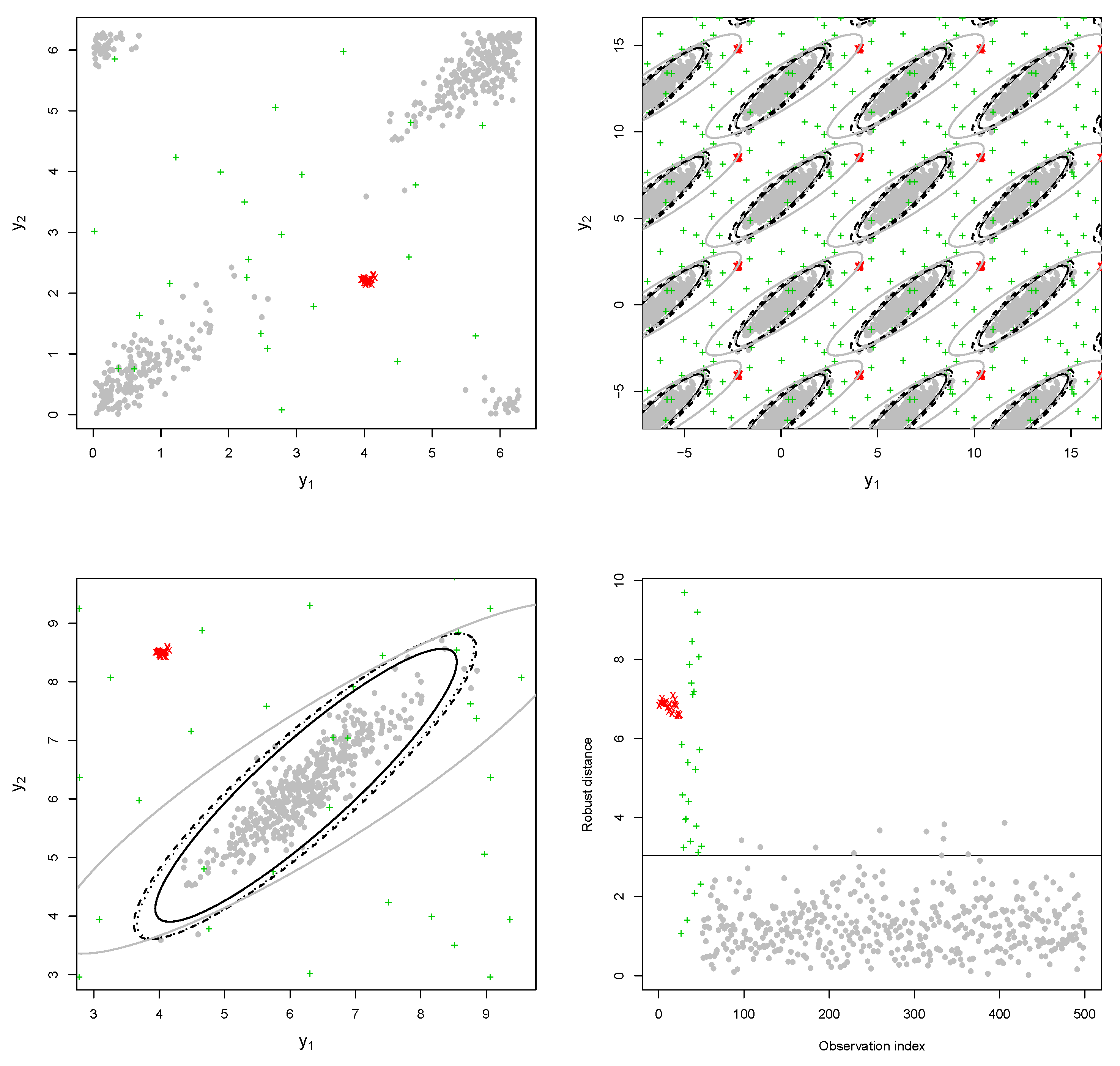
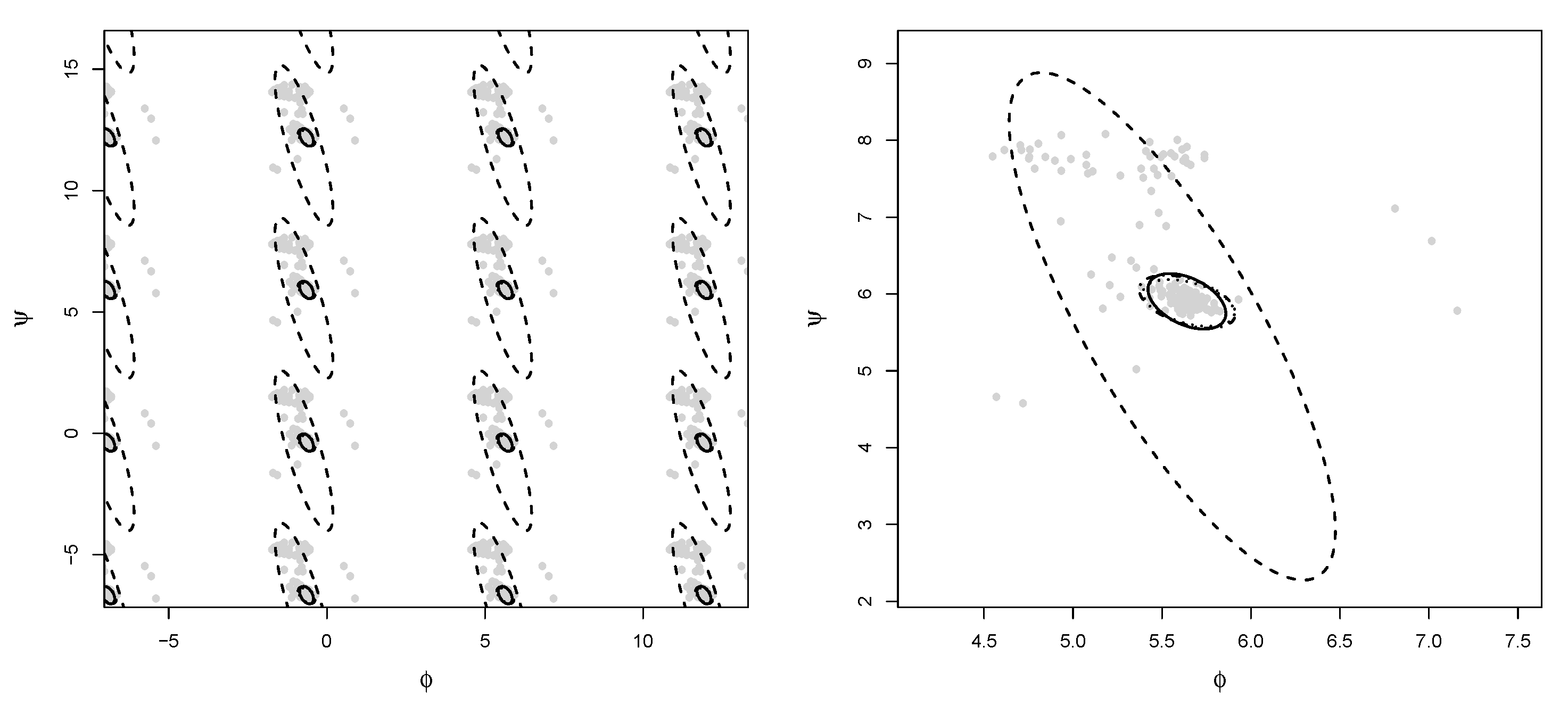
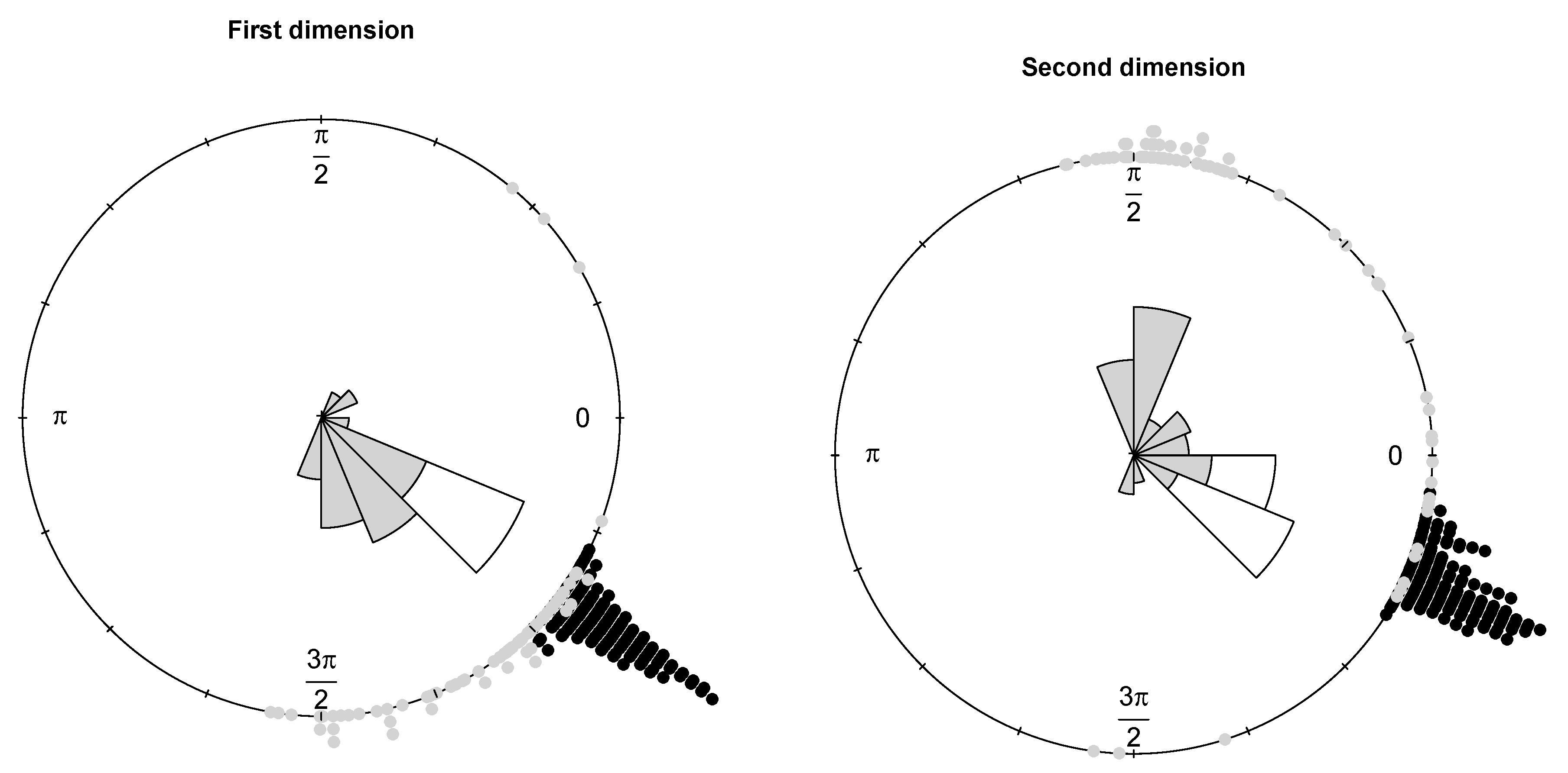
Example 1.

The bulk of the data (gray dots) has been drawn from a bivariate wrapped normal distribution with $\mathit{\mu }=\mathbf{0}$, $\mathsf{\Sigma }=0.1\ast R$, where R is a $2\times 2$ correlation matrix with off-diagonal elements equal to 0.7. Two types of contamination are considered. The first fraction of atypical data is composed by 25 scattered outliers along the circumference of the unit circle (denoted with a red cross). They have been selected so that their distances from the true model on the flat torus are larger than the 0.99-level quantile of the ${\chi }_p^2$ distribution. The remaining part is given by clustered outliers (green plus). The data are plotted in the left-top panel of Figure 1. Due to the intrinsic periodic nature of the data, one should think that the top margin joins the bottom margin, the left margin joins the right margin, and opposite corners join as well. Then, it is suggested to represent the circular data points after they have been unwrapped on a flat torus in the form $\mathit{x}=\mathit{y}+2\pi \mathit{j}$ for $\mathit{j}\in {\mathcal{C}}_{\mathcal{J}}$, respecting the cyclic topology of the data. Therefore, the same data structure is replicated according to the intrinsic periodicity of the data, as in the top-right panel of Figure 1. The bivariate fitted models are given in the form of tolerance ellipses based on the 0.99-level quantile of a ${\chi }_2^2$ distribution. A single data structure is given in the bottom-left panel with ellipses over-imposed. The bottom-right panel is a distance plot stemming from the WLE. The solid line correspond to the cut-off $\sqrt{{\chi }_{2;0.99}^2}$. Points above the threshold line are detected as outliers. All the considered outliers are effectively spotted after the robust CEM based on the WLE. In particular, the group of points corresponding to the clustered outliers is well above the cut-off. Similar results stem from the use of MM-estimation and impartial trimming. Figure 2 gives the fitted marginals on the circumference: The robust fits are able to recover the true marginal density on the circle, whereas the maximum likelihood fitted density has been flattened and attracted by outliers.

Example 2.

The data have been generated according to the procedure described in [8]: For a fixed condition number $CN=20$, we obtained a random correlation matrix R. Then, R has been converted into the covariance matrix $\mathsf{\Sigma }=D^{1/2}R{D}^{1/2}$, with $D=\mathrm{diag}\left({\sigma }^2{\mathbf{1}}_2\right)$, $\sigma =\pi /4$, and ${\mathbf{1}}_p$ denotes a p-dimensional vector of ones. Then, 25 outliers (red cross) have been added in the direction of the smallest eigenvalue of the covariance matrix [9], whereas the remaining 25 outliers have been sampled from a uniform distribution on $[0,2\pi ]$ (green plus).

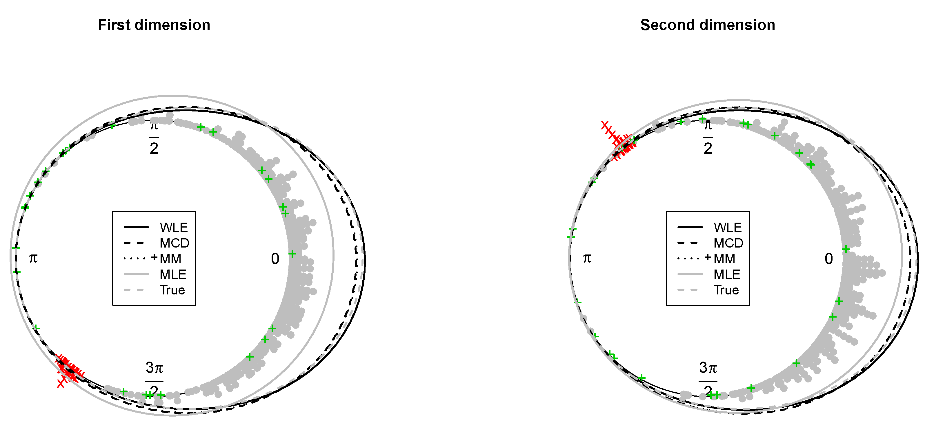
The data and the fitted models are given in Figure 3. The distance plot stemming from WLE is given in the bottom-right panel of Figure 3. The fitted and true marginals are given in Figure 4. As before, maximum likelihood does not lead to a reliable fitted model and does not allow to detect outliers because of an inflated fitted variance-covariance matrix. In contrast, the occurrence of outliers does not affect robust estimation. The robust methods lead to detect the point mass contamination since all corresponding points are well above the cut-off line, as are most of the noisy points added in the direction of the smallest eigenvalue of the true variance-covariance matrix.

6. Numerical Studies

In this section, we investigate the finite sample behavior of the proposed robust CEM algorithms through a simulation study with $N=500$ replicates. In particular, we consider MM-estimation with a 50% breakdown point and 95% shape efficiency, the WLE with a symmetric chi-square RAF and impartial trimming with 25% trimming and reweighting based on the 0.975–level quantile of the ${\chi }_p^2$ distribution, denoted as MCD. These methods have been compared to the MLE, evaluated according to the classical CEM algorithm. In all cases we set $J=3$. The data generation scheme follows the lines already outlined in the second synthetic example: Data are sampled from a $W{N}_p(\mu ,\mathsf{\Sigma })$ distribution, with $\mu =0$ and $\mathsf{\Sigma }=D^{1/2}R{D}^{1/2}$, where R is a random correlation matrix and $D=diag\left(\sigma {\mathbf{1}}_p\right)$. Contamination has been added by replacing a proportion $ϵ$ of randomly chosen data points. A couple of outliers configurations have been taken into account:

• Scattered: outlying observation are generated from a uniform distribution on ${[0,2\pi )}^p$.
• Point-mass: observations are shifted by an amount $k_{ϵ}$ in the direction of the smallest eigenvector of $\mathsf{\Sigma }$.

We considered dimensions $p=2,5$, sample sizes n = 100,500, $\sigma =\frac{\pi }{4},\frac{\pi }{2}$, contamination level $ϵ=10\%,20\%$, and contamination size $k_{ϵ}=\frac{\pi }{2},\pi$. Initial values are obtained by subsampling based on 20 starting values. The best solution at convergence is selected according to the criteria outlined in Section 3.6.

The accuracy of the fitted models is evaluated according to:

(i)

The average angle separation:

$$AS\left(\widehat{\mathit{\mu }}\right)=\frac{1}{p}\sum _{i=1}^p(1-cos\left({\widehat{\mathit{\mu }}}_i{\mathit{\mu }}_i\right)),$$

which ranges in $[0,2]$, for the mean vector;

(ii)

The divergence:

$$\Delta \left(\widehat{\mathsf{\Sigma }}\right)=trace\left(\widehat{\mathsf{\Sigma }}{\mathsf{\Sigma }}^{-1}\right)-log\left(\right|\widehat{\mathsf{\Sigma }}{\mathsf{\Sigma }}^{-1}\left|\right)-p,$$

for the variance-covariance matrix.

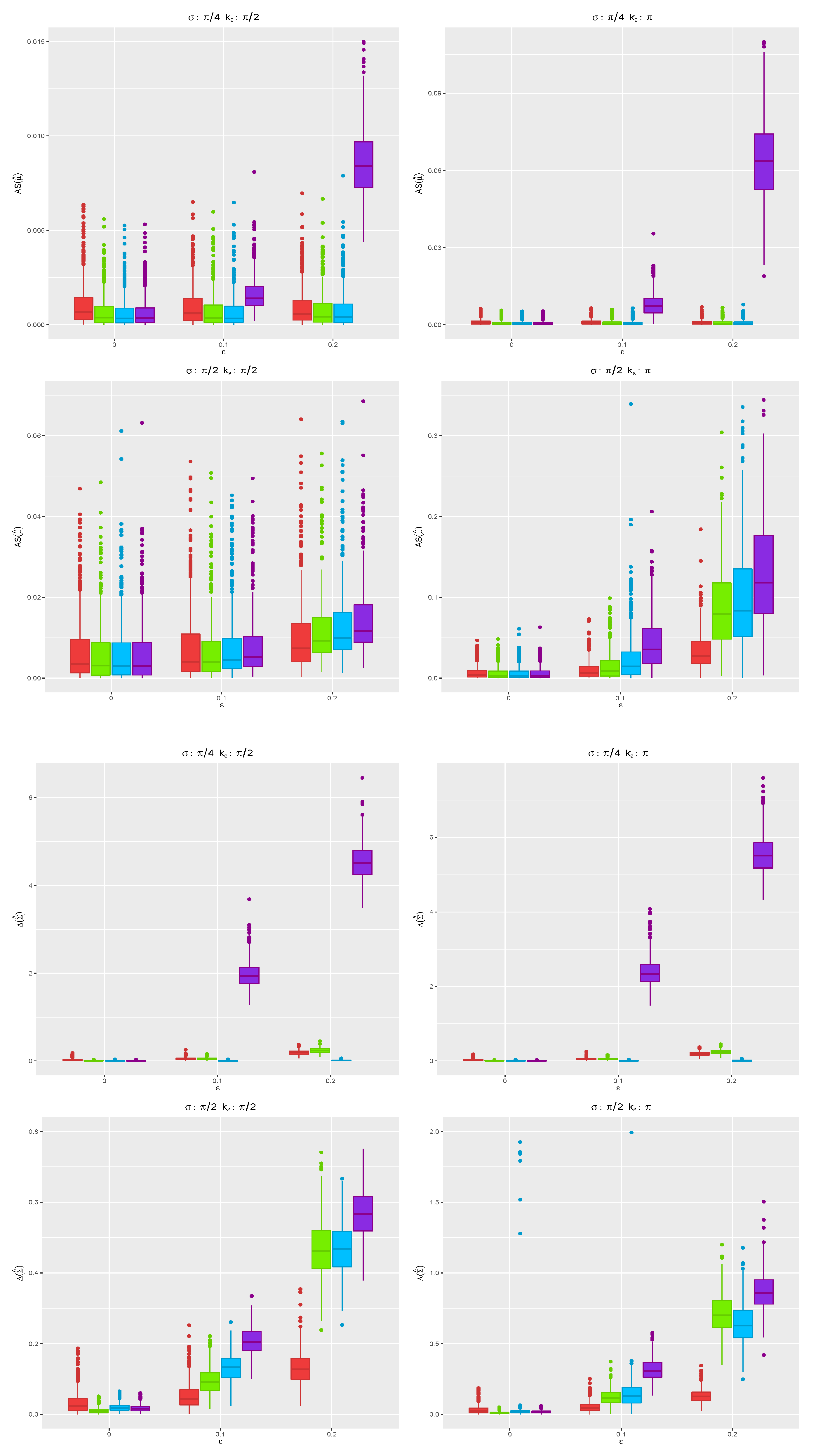
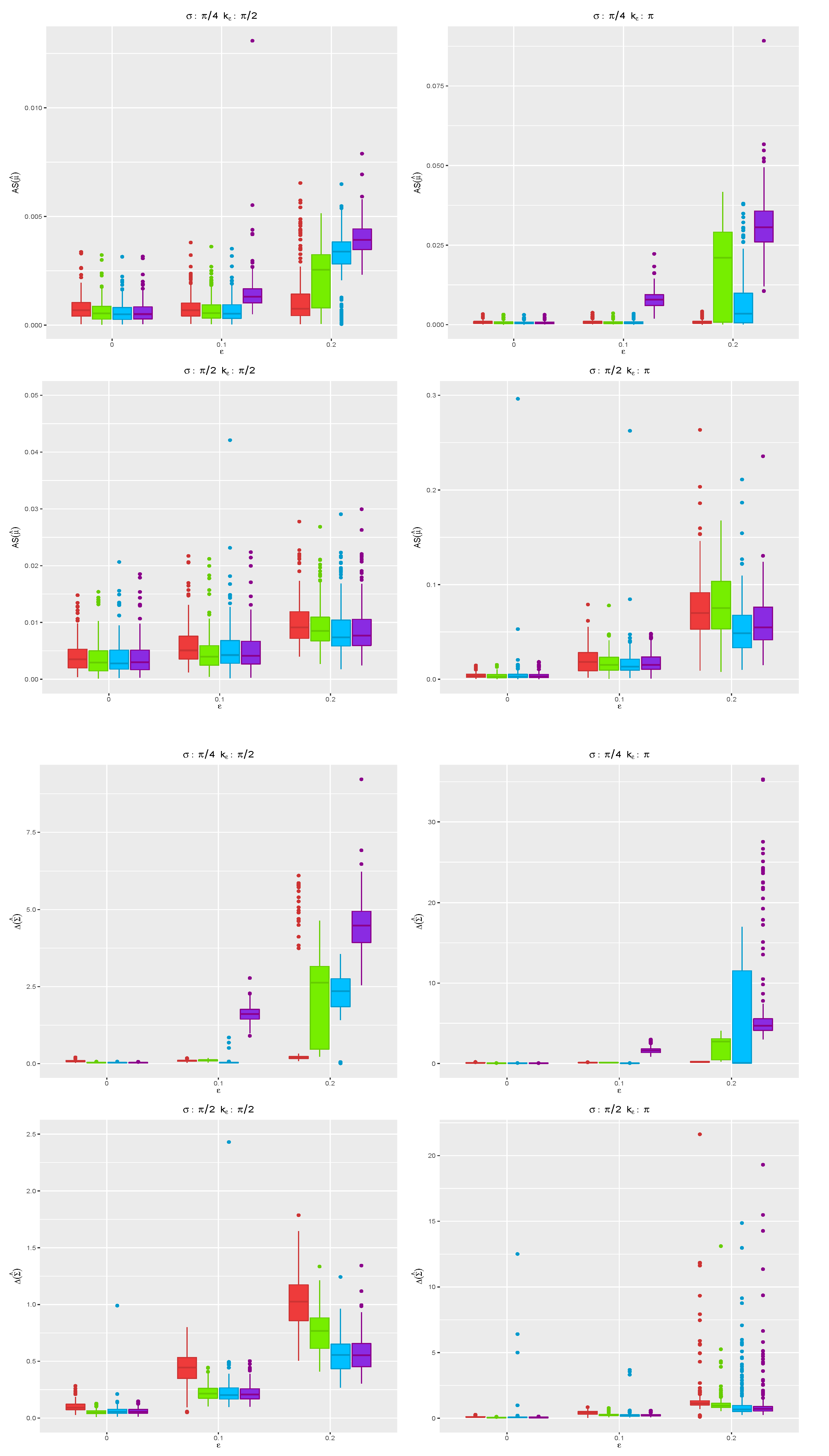
Here, we display the results for the scenario with $n=500$. Figure 5 shows the boxplots for the angle separation and divergence computed using the MCD (red), MM (green), WLE (blue), and MLE (violet) for all the replicates when $p=2$, while the case $p=5$ is given in Figure 6. Under the true model, the robust CEM gives results close to those stemming from the MLE. In contrast, in the presence of contamination in the data, the proposed robust CEM algorithm achieves a completely satisfactory accuracy, while the MLE deteriorates, especially when the contamination level increases. When $p=2$, the MCD shows the best performance among the robust proposals for the more challenging cases with $\sigma =\pi /2$, when outliers are not well separated from the bulk of genuine data points. The same is not true for $p=5$: The presence of outliers over all the p dimensions needs a different tuning of robust estimators.

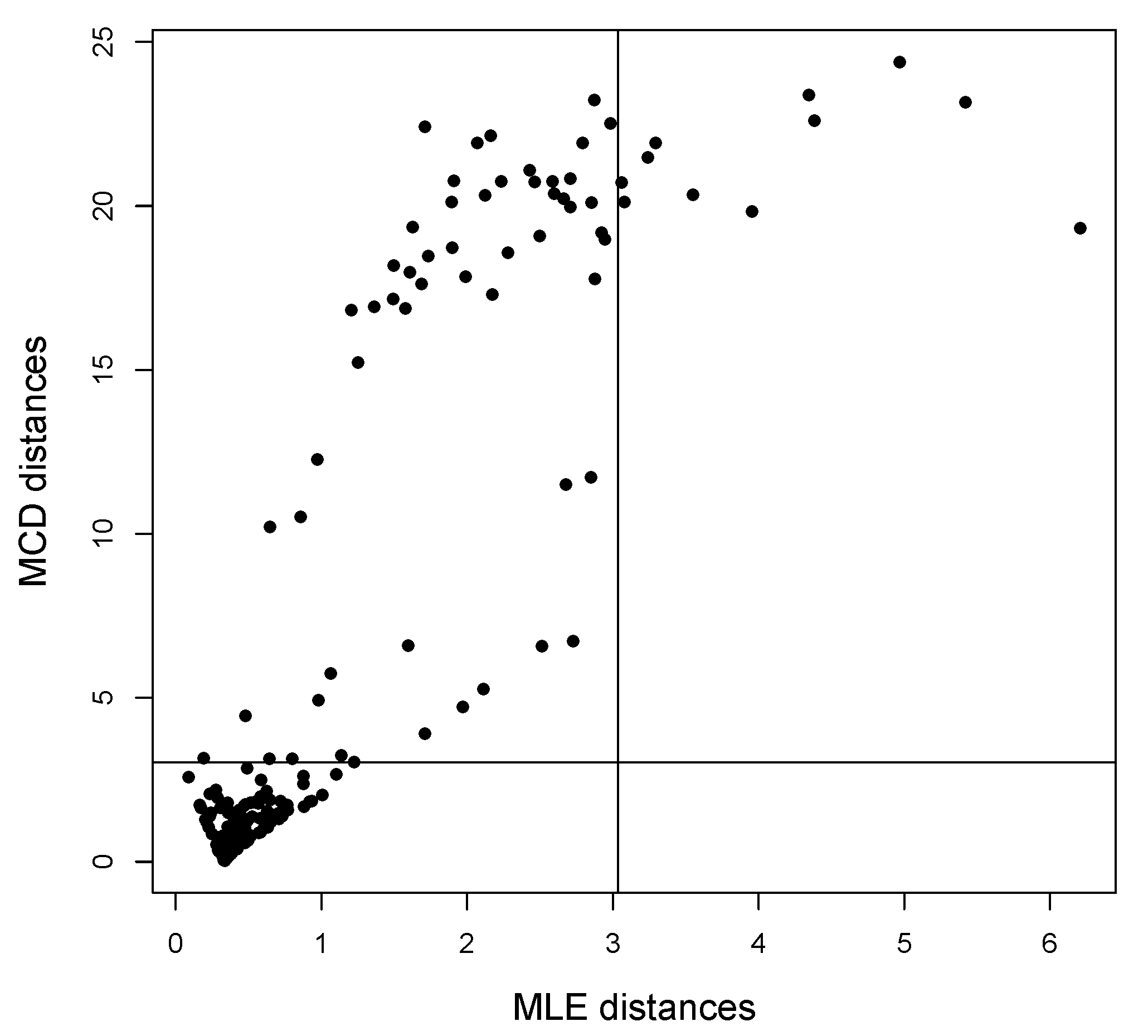
We also investigated the reliability of the proposed outlier detection rule (9) in terms of swamping and masking. The entries in

Table 1. Median values of type–I error rate for $p=2$ and $\alpha =5\%$.

			$\mathit{n}=100$				$\mathit{n}=500$
$\mathit{ϵ}$	$\mathit{\sigma }$	${\mathit{k}}_{\mathit{ϵ}}$	MCD	MM	WLE	MLE	MCD	MM	WLE	MLE
0	$\frac{\pi }{4}$	$\frac{\pi }{2}$	0.05	0.05	0.07	0.05	0.05	0.05	0.06	0.05
		$\pi$	0.05	0.05	0.07	0.05	0.05	0.05	0.06	0.05
	$\frac{\pi }{2}$	$\frac{\pi }{2}$	0.04	0.03	0.05	0.03	0.04	0.03	0.04	0.04
		$\pi$	0.04	0.03	0.05	0.03	0.04	0.03	0.04	0.04
0.1	$\frac{\pi }{4}$	$\frac{\pi }{2}$	0.02	0.02	0.07	0.01	0.02	0.02	0.05	0.01
		$\pi$	0.02	0.02	0.07	0.01	0.02	0.02	0.05	0.01
	$\frac{\pi }{2}$	$\frac{\pi }{2}$	0.01	0.01	0.02	0.01	0.01	0.01	0.01	0.01
		$\pi$	0.01	0.01	0.02	0.01	0.01	0.02	0.02	0.01
0.2	$\frac{\pi }{4}$	$\frac{\pi }{2}$	0.00	0.01	0.06	0.00	0.01	0.01	0.04	0.01
		$\pi$	0.00	0.01	0.06	0.01	0.01	0.01	0.04	0.01
	$\frac{\pi }{2}$	$\frac{\pi }{2}$	0.00	0.00	0.01	0.00	0.00	0.01	0.01	0.01
		$\pi$	0.01	0.00	0.01	0.00	0.01	0.01	0.01	0.01

give the median percentage of type–I errors, that is of genuine observations of wrongly declared outliers, whereas

Table 2. Median values of type–II error rate for $p=2$ and $\alpha =5\%$.

			$\mathit{n}=100$				$\mathit{n}=500$
$\mathit{ϵ}$	$\mathit{\sigma }$	${\mathit{k}}_{\mathit{ϵ}}$	MCD	MM	WLE	MLE	MCD	MM	WLE	MLE
0.1	$\frac{\pi }{4}$	$\frac{\pi }{2}$	0.10	0.10	0.00	0.10	0.08	0.08	0.06	0.14
		$\pi$	0.10	0.10	0.00	0.15	0.08	0.08	0.06	0.16
	$\frac{\pi }{2}$	$\frac{\pi }{2}$	0.30	0.30	0.30	0.70	0.30	0.32	0.42	0.76
		$\pi$	0.35	0.30	0.30	0.70	0.30	0.28	0.32	0.78
0.2	$\frac{\pi }{4}$	$\frac{\pi }{2}$	0.10	0.10	0.05	0.70	0.11	0.10	0.06	0.69
		$\pi$	0.10	0.10	0.05	0.70	0.11	0.10	0.06	0.71
	$\frac{\pi }{2}$	$\frac{\pi }{2}$	0.80	0.85	0.80	0.85	0.84	0.84	0.83	0.85
		$\pi$	0.80	0.80	0.80	0.85	0.81	0.83	0.82	0.84

gives the median percentage of type–II errors, that is of non-detected outliers. The testing rule has been applied for a significance level $\alpha =0.05$. We only report the results for $p=2$. Swamping derived by the robust methods is always reasonable. Their masking error is satisfactory but for the scenario with $\sigma =\pi /2$ and $ϵ=20\%$. Actually, in this case the outliers are not well separated from the group of genuine points. In contrast, the type-II error stemming from the MLE is always unacceptable. In summary, MM, MCD, and WLE performs in a satisfactorily equivalent fashion for the task of outlier detection, as long as outliers exhibit their own pattern different from the rest of the data.

7. Real Data Examples

7.1. Protein Data

The data set contains bivariate information about $n=223$ pairs of dihedral angles $(\varphi ,\psi )$ in a protein between three consecutive Alanine amino acids. This data set was extracted from the vast Protein Data Bank [40] and is available from the R package CircNNTSR [41]. We compare the results from maximum likelihood estimation with those stemming from the robust CEM based on MM-estimation (0.5 breakdown point and 0.95 shape efficiency), weighted likelihood estimation (Hellinger distance RAF and bandwidth set equal to 0.5), and MCD-type impartial trimming (with 0.5 level of trimming and reweighting). The classical and robust CEM have been run with $J=3$ and initialized from 20 different starting values obtained through subsampling. The data and the fitted models are shown in Figure 7. In the left panel the data are displayed on a flat torus; in the right panel the unwrapped data corresponds to $\mathit{j}=(0,0)$. In both panels the fitted models are represented through tolerance ellipses based on the 0.99-level quantile of the ${\chi }_2^2$ distribution. The data are non homogeneous in the sense that at least a couple of distinct clusters can be well identified. Maximum likelihood is not able to catch such different patterns in the data. In contrast, all the robust methods are successful in unveiling the presence of different structures, otherwise undetectable: The tolerance ellipses corresponding to WLE, reweighted MCD, and MM-estimation are almost indistinguishable. Let us consider the output from the robust CEM based on the reweighted MCD. The results from the other techniques are very similar and not reported here. According to an outlier testing rule performed at a significance level $\alpha =0.01$, the bulk of the data is composed by about $72\%$ of the points, whereas the remaining $28\%$ are outliers. This classification has been displayed in Figure 8: Outlying $\varphi$ angles exhibit a large spread and are mainly located on the arc between $3\pi /2$ and $7\pi /4$; outliers in the $\psi$ dimension are mainly clustered close to $\pi /2$, far from the bulk of the data. Group-wise rose diagrams have been also added to highlight further the differences. Figure 9 shows a distance-distance plot, in which MLE-based Mahalanobis distances are plotted against their MCD based counterpart. The horizontal and vertical lines give the ${\chi }_{0.99,2}^2$ cut-off. The inspection of the distance-distance plot shows that the robust CEM detects at least a couple of sub-groups in the data that are largely hidden to maximum likelihood.

7.2. RNA Data

We analyze data about seven independent torsion angles measured for each nucleotide in RNA molecules: Six dihedral angles and one angle for the base. Data have been taken from the large RNA data set [42]. The original data was split into 23 clusters. Here, we consider data from the third cluster, whose size is 232, merged with the 28 measurements from the twenty-third cluster, for a final sample size $n=260$. The reader is pointed to [8] for maximum likelihood estimation in each cluster. It is plausible to suppose that the data from cluster 23 stand as outliers with respect to those data from cluster 3, since they have received a different classification. Indeed, the results displayed in Figure 10 support the assumption that the points from cluster 23 are clearly spotted by the reweighted MCD (with $25\%$ trimming), as well as the WLE (with Symmetric Chi-Square RAF and $h=0.01$) and the MM- (0.5 breakdown and 0.85 shape efficiency) based robust CEM algorithms, whereas they are masked by maximum likelihood. Then, the proposed robust approach is able to discriminate between the two groups and reveal the underlying clustered structure of the data.

8. Concluding Remarks

We proposed a methodology to fit a multivariate wrapped normal distribution to circular data lying on a p—dimensional torus in the presence of outliers. Outliers could originate from wrong measurements, rare directions, or the presence of sub-groups. The technique performed satisfactorily with synthetic and real data, both for the task of parameter estimation and outlier detection. The estimation algorithm involves a modification of the classical CEM used to perform maximum likelihood estimation, in which the wrapping coefficients are considered as latent variables. At the M-step of the proposed robust CEM, we solve a set of complete data estimating equations that define robust estimators of a multivariate location and scatter, with particular emphasis on weighted likelihood, MM-estimation, and impartial hard trimming. This approach allows us to measure outlyingness according to the Mahalanobis distance of the complete data to the robust fit. The methodology is particularly appealing for moderate to large dimensions. As a final remark, we again point out that the proposed approach can be extended to the family of elliptically symmetric wrapped distributions in a more general framework.