Analysis of ‘Pre-Fit’ Datasets of gLAB by Robust Statistical Techniques

Abstract

The GNSS LABoratory tool (gLAB) is an interactive educational suite of applications for processing data from the Global Navigation Satellite System (GNSS). gLAB is composed of several data analysis modules that compute the solution of the problem of determining a position by means of GNSS measurements. The present work aimed to improve the pre-fit outlier detection function of gLAB since outliers, if undetected, deteriorate the obtained position coordinates. The methodology exploits robust statistical tools for regression provided by the Flexible Statistics and Data Analysis (FSDA) toolbox, an extension of MATLAB for the analysis of complex datasets. Our results show how the robust analysis FSDA technique improves the capability of detecting actual outliers in GNSS measurements, with respect to the present gLAB pre-fit outlier detection function. This study concludes that robust statistical analysis techniques, when applied to the pre-fit layer of gLAB, improve the overall reliability and accuracy of the positioning solution.

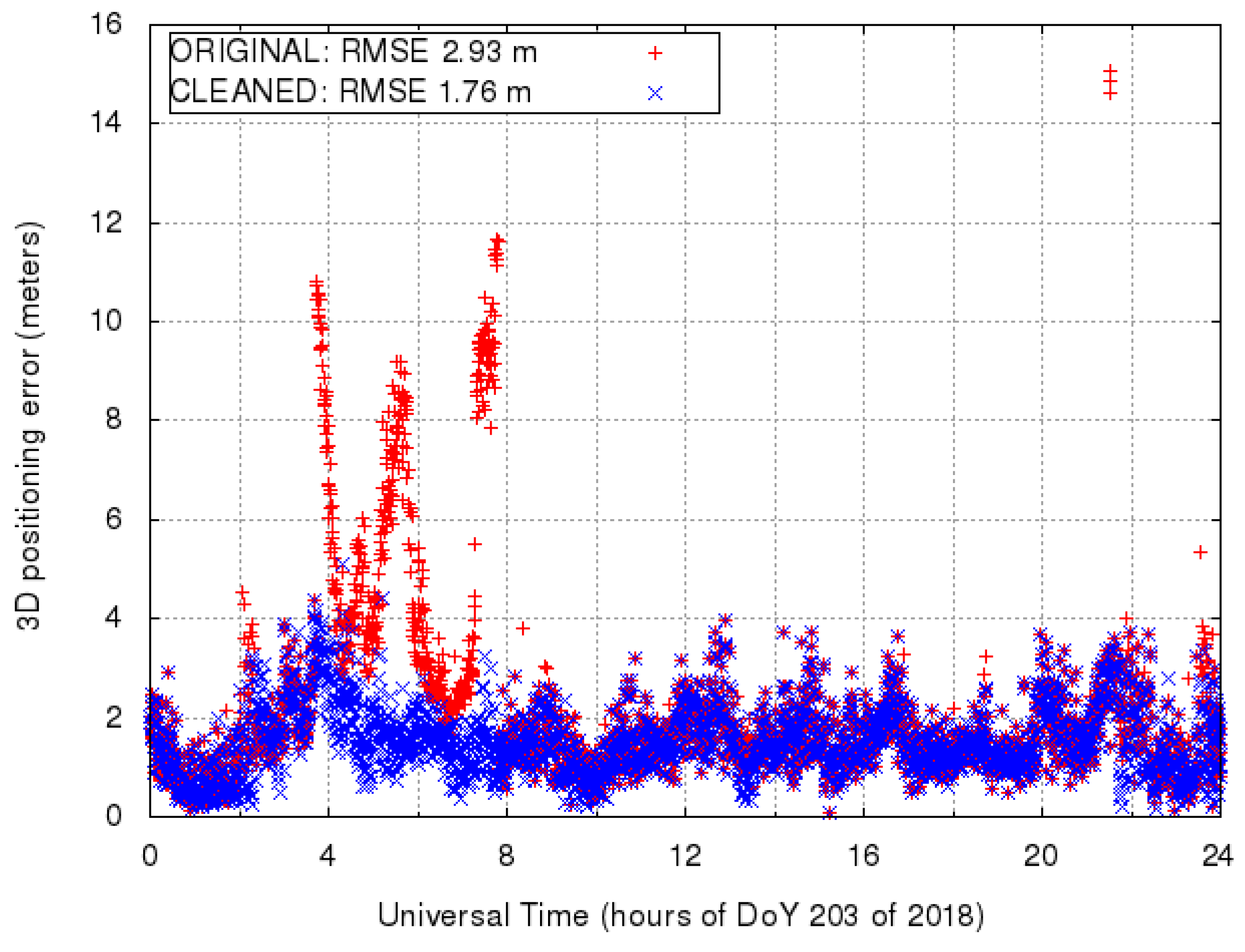
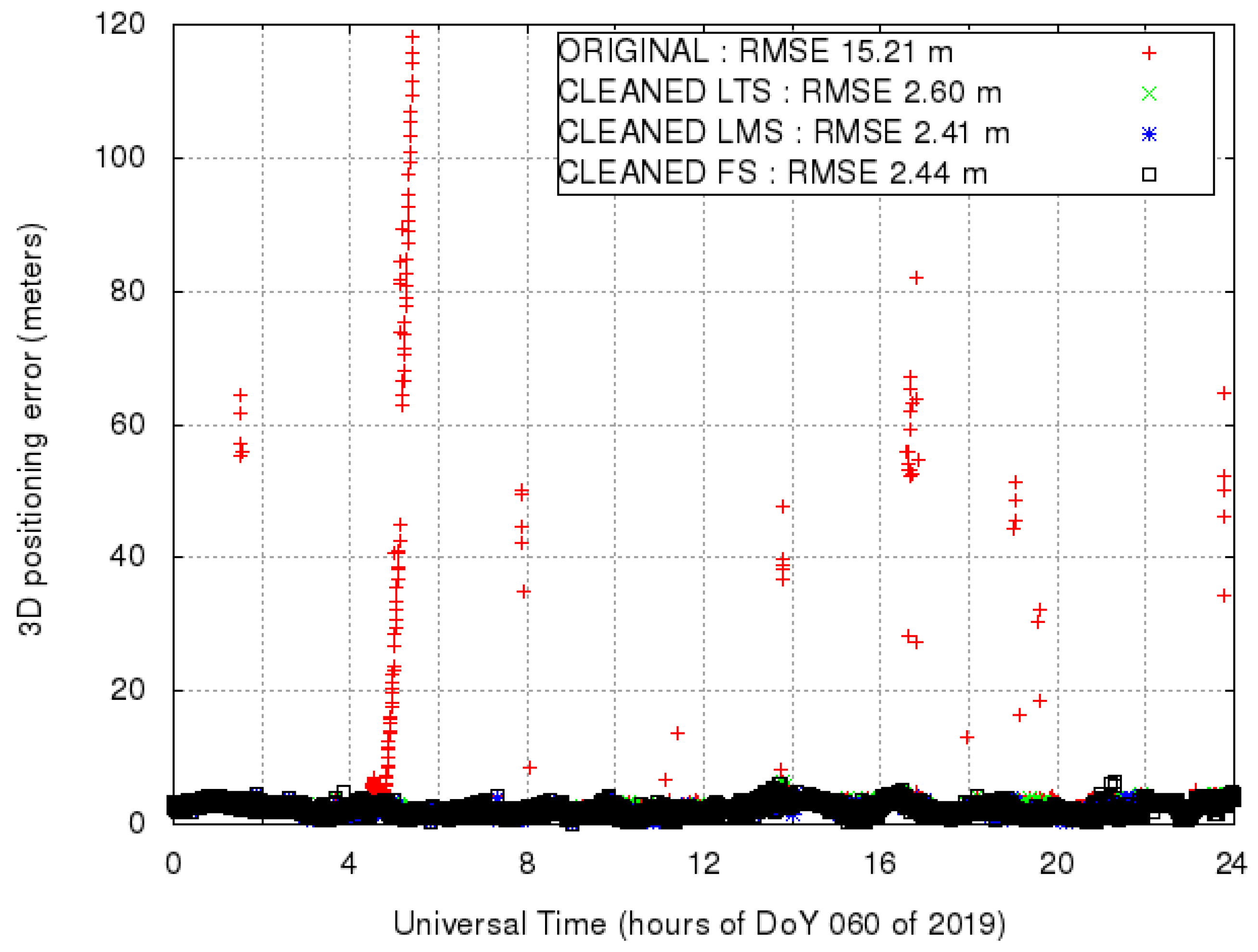
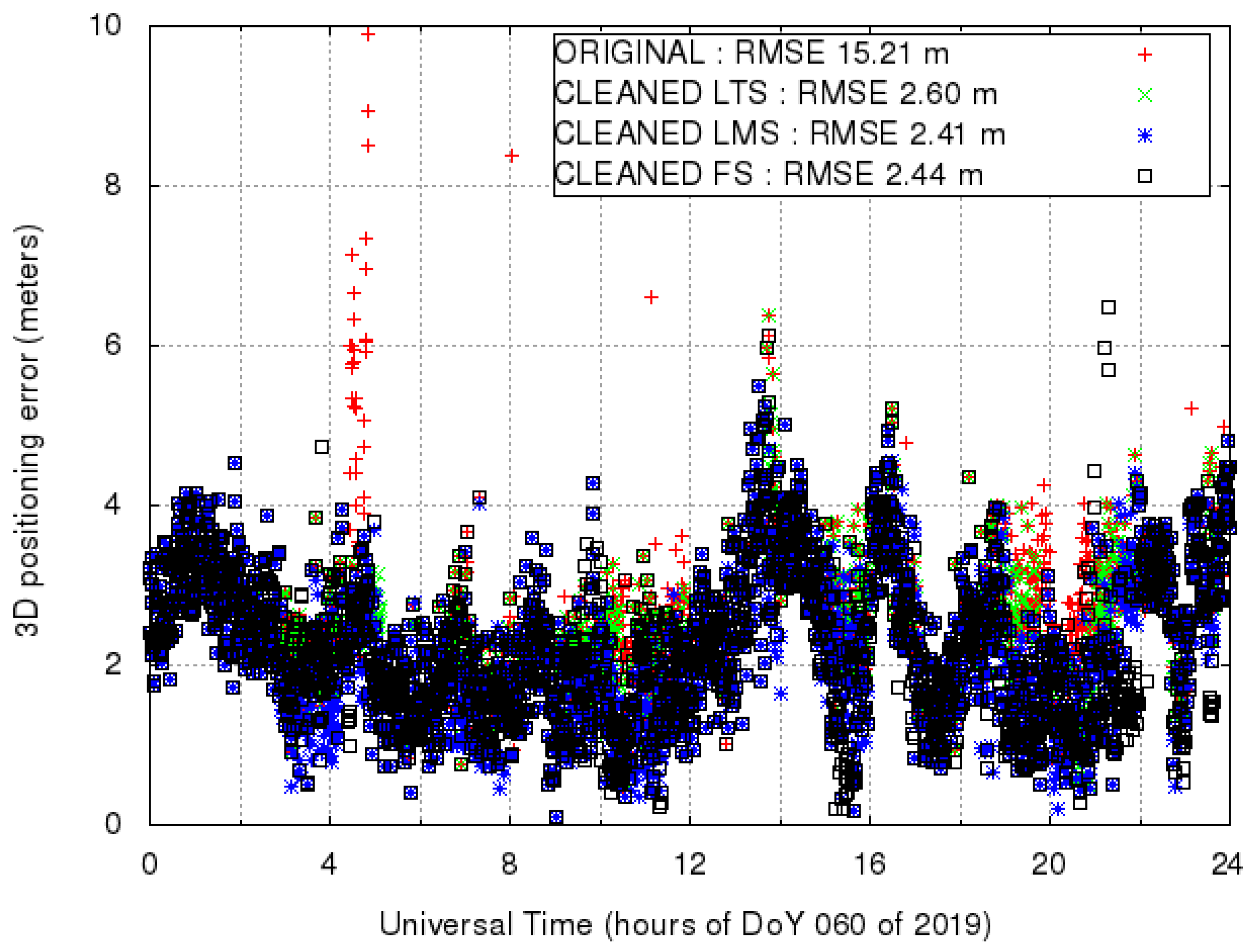
1. Introduction

The Global Navigation Satellite System (GNSS) provides positioning, velocity and timing (PVT) services to users equipped with appropriate hardware (i.e., an antenna and a receiver) [1]. There are four GNSS constellations that allow users to compute their PVT on a global basis (i.e., worldwide), two of which have already declared their full operational capability (FOC). Namely, the Global Positioning System (GPS, US Air Force), completed in 1994; the Global Navigation Satellite System (GLONASS, Russian Federal Space Agency) completed in 1995 (and restored in 2011). Two additional constellations are being completed and thus have not reached FOC: the BeiDou Navigation Satellite System (BDS, China National Space Administration) and Galileo (European Union). The Multi-GNSS Experiment (MGEX) [2] of the International GNSS Service (IGS) [3] monitors the rapid development of GNSS constellations. The processing of GNSS data is an essential part of PVT determination [4]. Once the receiver has acquired and demodulated the radio frequency GNSS signals from the antenna, it generates the code and carrier-phase measurements (the so-called observables). Then, these observables undergo a series of processing steps so that they can be used to estimate the PVT of the GNSS receiver by means of least squares (LS) or the Kalman filter [5], among other methods. Several software packages exist that are capable of processing GNSS data automatically.

The GNSS LABoratory tool (gLAB) is an advanced educational multi-purpose software used for processing and analyzing GNSS data [6]. The research group of Astronomy and Geomatics (gAGE) started developing gLAB in 2009, in the context of the European Space Agency (ESA) educational program on satellite navigation (EDUNAV). After one decade of evolution, gLAB capabilities include the most common GNSS navigation modes: stand-alone positioning, differential-mode, and augmented positioning with integrity. gLAB is open source and allows to fully control its internal processing through its many configuration options. This is a great advantage with respect to proprietary GNSS data processing programs produced by receiver manufacturers, which do not allow any modification and hence, from the user/scientific point of view, are black boxes. The processing core of gLAB is structured in five highly configurable modules. These modules mimic the aforementioned processing steps, being quite standard in commercial software receiver packages. For completeness, those modules are briefly summarized as follows:

• The INPUT module: interfaces with the standard input files and the rest of the program. It implements all the reading capabilities and stores the data in the memory structures of gLAB, that contain, as minimum, the raw measurements and the pseudo-Keplerian elements that allow computing the GNSS satellite position and its clock offset.
• The PREPROCESSING module: checks and selects the read data to be further processed. It detects cycle-slips (i.e., discontinuities) in the carrier-phase measurements, decimates the input data to a lower processing rate (if required) and selects which satellites and which constellations are used in the following modules, among other functions.
• The MODELLING module: provides an accurate model of the measurements from the receiver to each tracked satellite. In this regard, the pseudorange measurements $P_{rec}^{sat}$ can be written according to [4] as

  $$P_{rec}^{sat}={\rho }_{rec}^{sat}+c(\delta t_{rec}-\delta t^{sat})+Tro{p}_{rec}^{sat}+Io{n}_{rec}^{sat}+IF{B}^{sat}+{\epsilon }_{rec}^{sat};sat=1,\dots ,n$$

  (1)

  where ${\rho }_{rec}^{sat}$ is the geometric distance between the receiver and the satellite, c stands for the velocity of light, $\delta t_{rec}$ and $\delta t^{sat}$ are the receiver and satellite clock offsets, $Tro{p}_{rec}^{sat}$ and $Io{n}_{rec}^{sat}$ are the propagation delays occurring at the troposphere and ionosphere respectively, $IF{B}^{sat}$ is the satellite inter-frequency biases (IFB), and ${\epsilon }_{rec}^{sat}$ accounts for the measurement noise. The output of the MODELLING module are the pre-fit residuals, i.e., the difference between the preprocessed measurements and the sum of the model terms:

  $$prefi{t}_{rec}^{sat}=P_{rec}^{sat}-Pmode{l}_{rec}^{sat};sat=1,\dots ,n$$

  (2)
  Considering the model terms described in the standard point positioning (SPP) [7], the pre-fit residuals result in:

  $$prefi{t}_{rec}^{sat}={\rho }_{rec}^{sat}+c\delta t_{rec}+{\epsilon }_{rec}^{sat};sat=1,\dots ,n$$

  (3)

  where Equation (3) contains four unknowns: three receiver coordinates in the geometric distance ${\rho }_{rec}^{sat}=\sqrt{({(x_{rec}-x^{sat})}^2+{(y_{rec}-y^{sat})}^2+{(z_{rec}-z^{sat})}^2)}$ and the time offset of the receiver clock offset $\delta t_{rec}$, with respect to GNSS time.
• The FILTER module: implements an extended Kalman filter to obtain the estimations of the receiver PVT from the pre-fit residuals. The filter outputs the values of the estimated unknowns together with its co-variance, as a measure of the uncertainty in the estimation process.
• The OUTPUT module: is in charge of printing intermediate and final results in a structured manner. This allows extracting useful and complete information at any point in the GNSS data processing chain.

Both in gLAB and in commercial software packages, PVT estimation can be deteriorated by outliers. Outliers can be intuitively defined as elements of a sample qualitatively distinct as ‘bad’ compared to the majority of the sample considered as ‘good’. Note that it is not said that outliers are ‘wrong’ data; they are data needing a ‘careful look’, since their ‘being distinct’ from the majority could lead to unreliable estimates. Outlier detection, by a comparative or quantitative evaluation of their quality of ‘being distinct’, is a central component of PVT estimation.

The aim of the present work was to improve the outlier detection capabilities of gLAB by working at the intermediate step between the MODELLING and the FILTER modules. To this aim, we considered as basic dataset the pre-fit residuals as in Equation (2) above. In this GNSS context, outliers can be more precisely defined as pre-fit residual values from a particular satellite that are too different from the pre-fit residuals median (computed including all satellites). Note that by pre-fit residuals we mean something distinct from residuals in regression theory; the different use of the word residuals should be clear from the context. The most common reason for the presence of outliers in the pre-fit residuals is the multipath effect, when GNSS signals from low-elevation satellites reach the antenna along multiple paths, following a reflection in the ground or surrounding structure. Other outlier sources are the malfunctioning of the receiver or satellite hardware. For the latter, the ground segment (GS) of each constellation constantly monitors the status of its satellites using a worldwide distribution of permanent stations. Thus, the GS can inform users of satellite anomalies by means of the healthy flag broadcast in the navigation message that is typically refreshed every two hours. In contrast, anomalies at one particular isolated receiver are more difficult to detect, as there is no redundancy of measurements. In this case, receiver autonomous integrity monitoring (RAIM) must be applied, following [8]. In the simplest form of position computation, as described in standard point positioning (SPP) [7], the pre-fit residuals of all satellites in view are fit by ordinary least squares, OLS, to three coordinates and one time-offset unknowns in an over-determined system of equations. The severity of outlier mis-detection depends on the magnitude of the outlier, on satellite geometry and on the user application. Safety of life (SoL) applications such as civil aviation or autonomous driving require specialized techniques to ensure positioning integrity (i.e., the measure of trust that can be placed in the correctness of the information supplied by a navigation system).

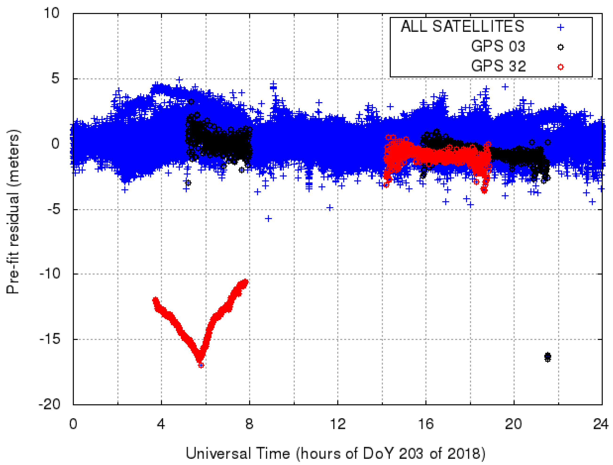
The qualitative distinction of outliers from the majority of the sample is immediately remarked when values are graphically represented in an appropriate way. For example, with reference to Figure 1, the ‘V-shaped’ set of points in the lower-left part is promptly perceived as ‘distinct from the majority of the sample’; the appropriate graphical representation of data remains today, when possible, an instrument for outlier detection by visual screening. When visual screening is not possible, or a fine-drawn decision has to be taken, automated techniques must be used. George Edward Pelham Box, in 1953, coined the term robust in relation to this need, but this (certainly older) concept was formalized in a proper discipline only later, starting from the mid-1960s. Roughly speaking, robust statistics can now be seen as an operational approach to the treatment of outliers; treatment that can range from the detection and elimination of outliers from the sample to some degree of mitigation of their effects on the choice and computation of estimators. The standard example of resistance to outliers of an estimator is given by comparing the effect of a single diverging value $y\to \infty$ on the sample mean and the sample median: the mean being immediately influenced by this value of y, while the median is resistant. The degree of resistance to the outliers of an estimator is represented by a parameter called breakdown point. The breakdown point of the sample mean is $0\%$ while the breakdown point for the median is $50\%$ since it can tolerate up to $50\%$ of ‘gross errors’ in data before diverging.

The use of robust statistics techniques for GNSS positioning is a growing field both in applications and in methodological aspects. Examples of the applications of robust statistics to positioning problems can be found in artificial intelligence [9] and geodesy [10]. Concerning the methodological aspects, an example of improvement of the SPP algorithm by using Huber M-estimators can be found in [11] while in [12] a form of robust Kalman filtering is used in the kinematic positioning component. These two methodological aspects can be referred to the MODELLING and FILTER modules of gLAB. To our knowledge, there are no other attempts in the literature to improve the position solution with robust statistics by exploiting the pre-fit residuals, i.e., by working at the connection between the MODELLING and the FILTER modules, as in the gLAB architecture.

The Flexible Statistics and Data Analysis (FSDA) toolbox [13] is a MATLAB module gathering a comprehensive set of statistical functions for the analysis of data. The original aim of this library of functions was to extend the MATLAB Statistics Toolbox with forward search analysis [14]. FSDA was subsequently extended and now includes all the main robust multivariate and regression tools, complemented by instruments for robust transformations and the interactive graphical exploration of data; it is available for Windows, Unix and MacOS platforms. (FSDA is copyright of the European Commission and the University of Parma. It is protected under European Union Public Licence (EUPL) [15], which is a free software licence granting recipients rights to modify and redistribute the code. FSDA is distributed through GitHub https://github.com/UniprJRC/FSDA—accessed on 15 May 2021— and the MATLAB community https://www.mathworks.com/matlabcentral/fileexchange/72999-fsda (accessed on 15 May 2021). A complete documentation with examples, datasets and tutorials is available at http://rosa.unipr.it/FSDA (accessed on 15 May 2021). A version of the suite with selected functionalities is also available in R at https://cran.r-project.org/web/packages/fsdaR/index.html (accessed on 15 May 2021) and in SAS, upon request to the JRC co-authors.) The analysis of pre-fit datasets reported in this article can be considered as our first attempt to apply robust statistical techniques as provided by the FSDA toolbox to PVT estimation.

After a description of the typical data and the problems to be faced in Section 2, with a first essay employing the traditional robust estimator least median of squares (LMS), we proceeded with the use of other FSDA functions for outlier detection still applied to relatively large samples of data. We did not use the full potential of FSDA, however, with the aim of comparing the results obtained at the beginning of Section 2 with LMS, we exploited least trimmed squares (LTS) and forward search (FS). In Section 3, a more precise analysis is done by considering samples whose cardinality is coherent with practical use: relatively short time windows of ten samples. In Section 4, the results of our analysis are summarized together with an indication of the directions of future work.

2. Structure of the Dataset and Preliminary Analysis

In this section, our study uses actual and publicly available data collected by a Javad ‘TRE_G3TH’ receiver, installed at a permanent station named KIR0 in Sweden. This is a standard geodetic-grade receiver as those usually found in the IGS network. (IGS data can be downloaded from the URL https://www.igs.org/data/—accessed on 15 May 2021.) The day of the experiment is the day of the year (DoY) 203 of 2018 (i.e., November 4th). Code pseudorange C1C measurements are logged with a period of 30 s, i.e., the sampling frequency is $1/30$ Hz, so we have 2880 epochs for the entire day. Each epoch contains a record, as in

Table 1. Excerpt from the pre-fit data table. Epoch in seconds, pre-fit and ranges in meters, elevation of the satellites in degrees.

Year	DoY	Epoch	Const.	Satellite	Pre-Fit	Measured Range	Modeled Range	Elevation
2018	203	30.00	GPS	30	1.1285	20,774,695.8820	20,774,694.7535	62.830
2018	203	30.00	GPS	7	0.5062	20,902,305.0420	20,902,304.5358	62.107
2018	203	30.00	GPS	5	0.6373	21,449,496.2580	21,449,495.6207	48.474
2018	203	30.00	GPS	13	0.0678	22,580,115.9500	22,580,115.8822	32.131
2018	203	30.00	GPS	27	−0.7367	23,106,933.9460	23,106,934.6827	23.969
2018	203	30.00	GPS	21	1.5017	24,496,859.0780	24,496,857.5763	19.849
2018	203	30.00	GPS	9	−0.6624	23,870,542.7020	23,870,543.3644	16.482
2018	203	30.00	GPS	8	−0.3127	24,198,683.3000	24,198,683.6127	14.795
2018	203	30.00	GPS	28	−1.0963	24,119,609.3400	24,119,610.4363	13.659
2018	203	30.00	GPS	16	0.3602	24,836,613.8360	24,836,613.4758	9.066
2018	203	77,520.00	GPS	9	0.6399	20,249,609.7060	20,249,609.0661	72.297
2018	203	77,520.00	GPS	23	−0.2187	21,521,386.7380	21,521,386.9567	50.623
2018	203	77,520.00	GPS	2	2.2097	22,539,967.2700	22,539,965.0603	37.848
2018	203	77,520.00	GPS	26	−0.6910	22,878,625.4080	22,878,626.0990	29.222
2018	203	77,520.00	GPS	16	−0.4619	22,622,817.8300	22,622,818.2919	29.130
2018	203	77,520.00	GPS	6	−0.2707	22,930,857.2880	22,930,857.5587	27.353
2018	203	77,520.00	GPS	7	0.1535	23,373,509.6060	23,373,509.4525	26.341
2018	203	77,520.00	GPS	29	0.0111	23,390,396.5840	23,390,396.5729	21.900
2018	203	77,520.00	GPS	5	−0.8185	23,946,589.7820	23,946,590.6005	16.100
2018	203	77,520.00	GPS	3	−16.2497	25,180,666.6940	25,180,682.9437	5.478

, for each satellite ‘visible’ and ‘tracked’ by the receiver.

Figure 1 illustrates the dataset which contains 24 h of pre-fit residuals, the output of the gLAB MODELLING module. This dataset contains both the pseudorange data corrected for some inconsistencies by the PREPROCESS module as briefly explained above, and the pseudorange data as predicted by the model. The computation of the pseudorange takes into account a number of model corrections following the SPP [7]. Note that, since we are using a fixed station with known coordinates and the satellite positions can be obtained from the broadcast navigation message of the satellites, we can compute the geometric range, the measured range in Table 1, for each of the tracked satellites. Then, the pre-fit residuals in Equation (3) turn into:

$$prefi{t}_{rec}^{sat}=c\delta t_{rec}+{\epsilon }_{rec}^{sat};sat=1,\dots ,n$$

(4)

Therefore, we should expect all pre-fit residuals from all satellites around the receiver clock offset value $c\delta t_{rec}$ to be only distinguishable by the noise of the measurement, ${\epsilon }_{rec}^{sat}$. Under normal conditions, this pseudorange noise reaches one meter at the high elevation of the satellite and few to several meters at low elevations.

In Table 1, an excerpt of two epochs from the complete data table of about 32,000 rows was reported; this table contains the satellite identifier and the pre-fit value, the plain difference between modeled and measured range. Note that at the first epoch, $30.00$, the order of magnitude of the pre-fit is about 1 meter for all satellites while at epoch 77,520, corresponding to hours $21h32$ in Figure 1, satellite 3 shows a pre-fit of about 16 m, probably caused by its low elevation. It is remarked that it is general practice not to consider in the solution of the positioning problem the satellites with ‘low’ elevation. gLAB, while operating in SPP mode, excludes by default satellites with an elevation below five degrees already in the PREPROCESSING module.

As a first essay with the dataset, we apply a LMS regression. The least median of squares estimator [16], described in more detail below, is historically among the first improvements of OLS and is implemented in FSDA by the LXS function. For LXS, we used a very conservative estimate, which was a Bonferroni-corrected [17] confidence level of $1-0.01/N\simeq 0.9999997$ where N is the number of observations—$32,000$ in the present case. The quantity $0.01/N\simeq 3\times {10}^{-7}$ can be considered as the probability to falsely declare a dataset as contaminated by outliers, when one is testing a large number of genuine datasets.

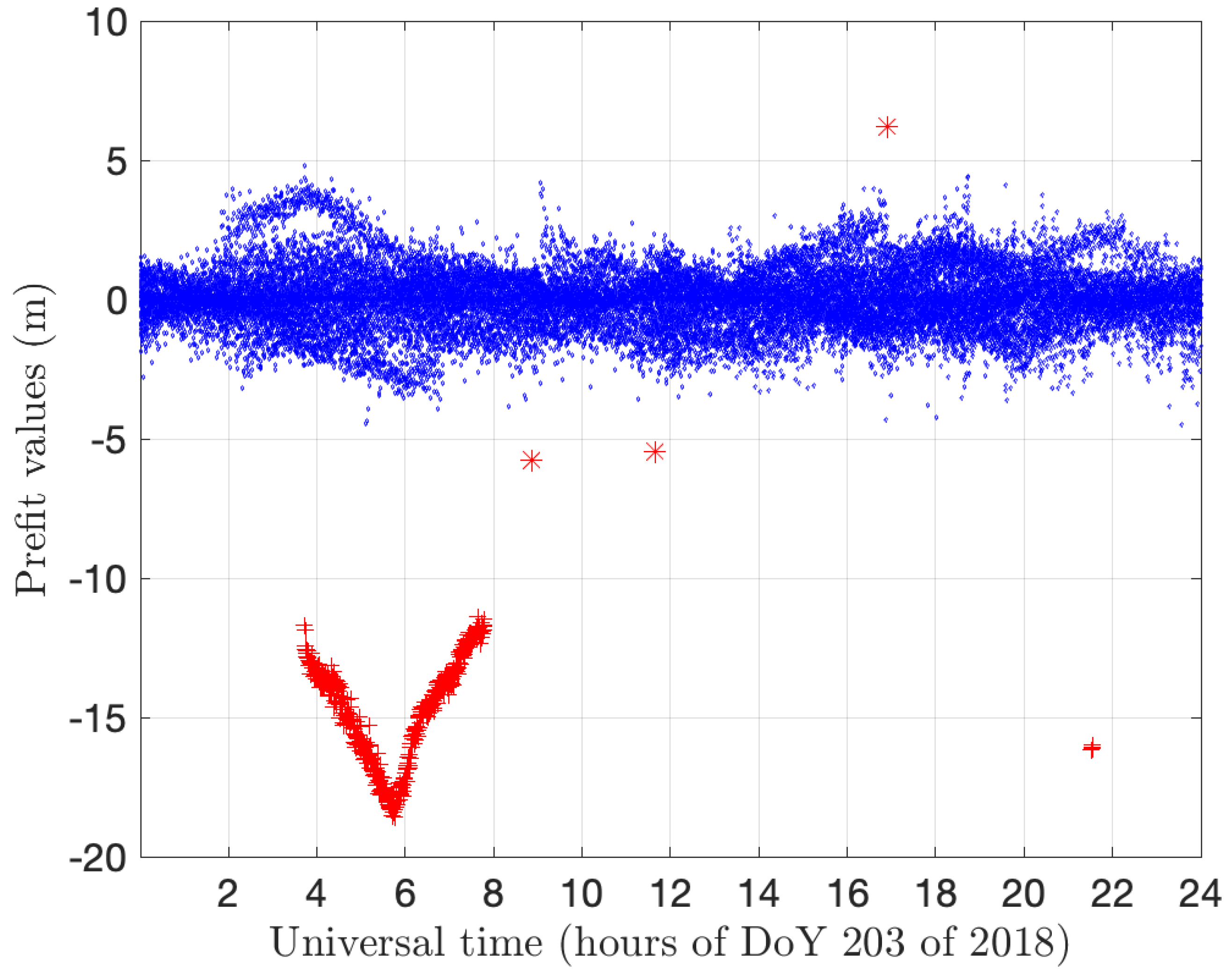
Figure 2 represents the outlier detection against LMS regression on 24 h of samples. The result with respect to other estimators, compared to LMS below in this section, will also be referred to in this Figure. With reference to Figure 2, the median pre-fit value for the whole dataset is $\approx 0.2183$ m. This rather small value indicates that the receiver is steering its clock to the GPS time, hence the receiver clock offset value $c\delta t_{rec}$ is close to 0 in Equation (4). The confidence interval found corresponds to about $\pm 5$ m. The two main groups of outliers were already evident by visual inspection in Figure 1. The “V-shaped” subset between hours 4 and 8 and the smaller group at about hour 22 are correctly identified by LMS. It is remarked that three distinct points at about hours 9, 12 and 17, very close to the limits of the confidence interval, are marked as outliers as well.

After this first essay on the data by LMS regression, three remarks can be made:

1

The outlier detection by visual screening and LMS regression with Bonferroni correction give comparable results;

2

Many robust methods (including those implemented in FSDA) are based on the assumption that the error component of the data analyzed is normally distributed. As the actual distribution can of course deviate from this common assumption, the confidence intervals are just ‘nominal’ in that the actual proportion of outliers detected can differ from the expected one.

3

The outlier detection algorithm presently used by gLAB, based on an heuristic threshold of 40 m:

• epochs := set of considered epochs;
• median := median of all pre-fit values in all epochs;
• for each epoch in epochs
•  for each satellite s in epoch
•   if | prefit(s) - median | > treshold
•    then discard satellite s in current epoch.

would have not detected the obvious outliers.

We now exploit, on the same dataset, two other estimators in addition to LMS above: least trimmed squares (LTS) and forward search (FS) as implemented in the FSDA toolkit. A detailed description of these methods with their actual implementation in FSDA can be found in [18]. The three robust regression methods build a linear model upon a set of data points composed of a vector of independent variables and one dependent variable. In our case, the data points would be structured, as shown in Table 1, as a vector of independent variables containing at least $(\mathrm{epoch},\mathrm{satellite},\mathrm{elevation})$ and with the pre-fit as the dependent variable. This would lead to a multi-variate distribution. We adopted a simplification, by considering the dataset as a sample from a uni-variate distribution allowing, in each epoch, for the repetition of the observations. While computing the linear model, we will not make distinctions among the individual satellites and we will not consider the elevation and other information included in the complete satellite’s messages.

The formal expression of the linear model (with intercept) is: $y=x{\theta }_1+{\theta }_2+\epsilon$, where $\epsilon$ represents a normally distributed error and x represents now the pairs $(\mathrm{epoch},\mathrm{satellite})$. Given n as the cardinality of the dataset, the set of data points will be ${\{x_i,y_i\}}_{1\le i\le n}$ with $y_i$ the pre-fit and $x_i$ representing a distinct pair $(\mathrm{epoch},\mathrm{satellite})$. The model is then computed by estimating with ${\widehat{\theta }}_i$ the parameters ${\theta }_i$ with respect to an appropriate objective function of the residuals: $r_i=y_i-(x_i{\widehat{\theta }}_1+{\widehat{\theta }}_2)$. The objective functions to minimize are, respectively, the sum of the squares of the residuals for OLS, the median of the squares of the residuals for LMS and the sum of the squares of a selected subset of the residuals for LTS [16]:

$$\underset{\widehat{\theta }}{min}\sum _i^n{r}_i^2\underset{\widehat{\theta }}{min}\underset{i}{\mathrm{median}}{r}_i^2\underset{\widehat{\theta }}{min}\sum _i^h{r}_{i:n}^2$$

(5)

where $r_{i:n}^2$ is the ordered set of the squared residuals $r_{1:n}^2\le r_{2:n}^2\le \dots \le r_{n:n}^2$ and h decides the appropriate subset of the points considered. Typically, for LTS, h is chosen with a breakdown point of 50% ($h=\lceil 0.5·n\rceil$) but it can be automatically increased according to the estimate of the residuals variance [16]. This re-weighting step allows keeping the desired robustness while increasing the efficiency of the estimator ${\widehat{\theta }}_i$.

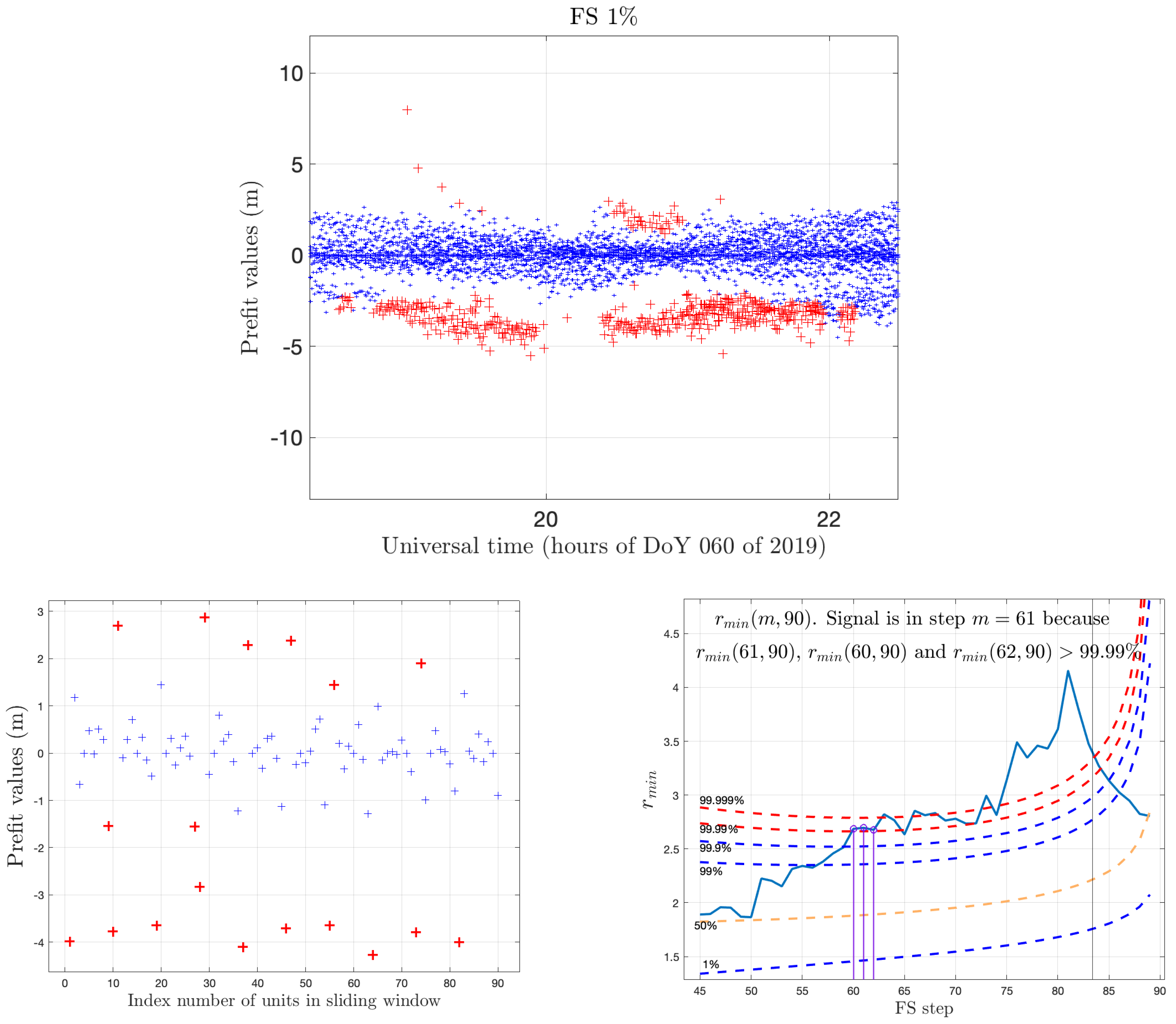
The forward search further exploits the re-weighting idea by building a sequence of data subsets of increasing size, and fitting a sequence of estimators ${\widehat{\theta }}_i^m,m_0\le m\le n,$ on them. More precisely, the forward process starts with a first small subset of $m_0$ data points, where ${\widehat{\theta }}_i^{m_0}$ is estimated with LMS or LTS. Note that $m_0$ can just be equal to the number of parameters, so the computational burden required by the initial LMS or LTS application is very limited. Then, the process continues by repeatedly computing ${\widehat{\theta }}_i^m$ with the OLS on the subsequent subsets of cardinality $m_0<m\le n$. Building the subset with the units with smallest $m+1$ squared residuals requires the computation of the $m+1$ order statistic in a vector of n numbers, which is known to have linear computational complexity (full or partial sorting of the residuals is not necessary). The process is iterated with OLS in steps $m:=m+1$ until the cardinality of the subsets reaches the cardinality n of the dataset. Figure 10 illustrates the signal detection mechanism of the FS using data in a window of 10 epochs.

Figure 2 reports the comprehensive result of the application of the estimators of LMS as above, LTS with re-weighting and Bonferroni correction and FS to the whole dataset. The outcomes of LTS and FS are identical and can be compared with the outcome of LMS. As in Figure 2, the difference between LMS on one side and LTS and FS on the other are in the three outliers close to the limits of the confidence interval of about 5 m. Overall, the three estimators give the same results while LTS and FS yield a somewhat different performance compared to LMS, in dependence of the judgment (outliers or main population) for the points at the border of the confidence interval.

3. Analysis with Time Windows

In this section, we further deepened our investigation by applying the previous methods to a sliding time window of ten epochs. The dataset used in this case belongs to the permanent station named HUEG, located in Germany, for DoY 060 of 2019 (i.e., March 1st). 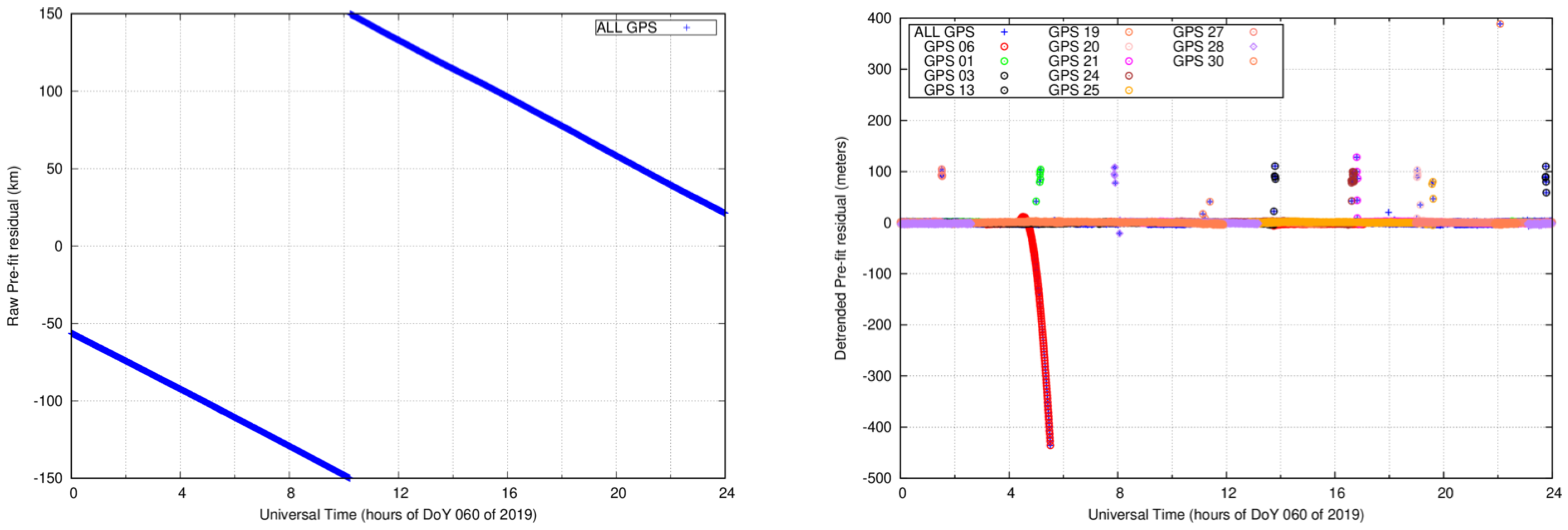Although the receiver is a Javad ‘TRE_G3TH’, the same model as the one used in the preliminary analysis of Section 2 above, the clock of the receiver (i.e., $\delta t_{rec}$ in Equation (4)) is not steered to GPS time, presenting a rapid drift as illustrated in the left plot of Figure 3. According to the interface control document (ICD) [19], the receiver clock offset can have any value within a $\pm 0.5$ ms (i.e., $\pm 150$ km). When it reaches the minimum (or maximum) limit, it must reset to remain within the prescribed range of $\pm 0.5$ ms Therefore, in order to analyze the pre-fit residuals containing such clock behaviors, a detrending procedure must be applied. Moreover, as a step towards real-time applications, in this section, we use a sliding window rather than analyzing the complete time window of 24 h at once.

Thus, in order to eliminate the clock drift prior to outlier detection, we performed a linear detrending to all pre-fit residuals. This detrending is obtained by subtracting the instantaneous median value at each epoch. The right plot of Figure 3 illustrates the result of such detrending. We can observe few outliers at some particular satellites that were hidden by the clock drift in the original ‘raw’ pre-fit residuals depicted in the left plot of Figure 3. While most of the outliers range within 100 m, GPS satellite 6 presents an outlier that reaches more than 400 m. This outlier is simultaneously observed in other permanent stations, thus it is attributable to some satellite anomaly. Indeed, the Notice Advisory to Navstar Users (NANU) number 2019029 [20] was issued, reporting that the GPS06 satellite was unusable that day.

We now apply the outlier detection algorithms based on LMS, LTS and FS to the HUEG dataset. With the aim of developing an efficient mechanism for outlier detection of pre-fit values, we chose a relatively small time window of ten epochs. That is, the window considers five minutes of data for each computation, sliding along the whole 24 h of observations. This choice is arbitrary and is done only as a kind of compromise between the need for a decision about unreliable satellites within ‘few’ minutes and having a meaningful set of data. The outliers, computed by using data of the whole window, are assigned to the epoch ‘entering’ the window itself.

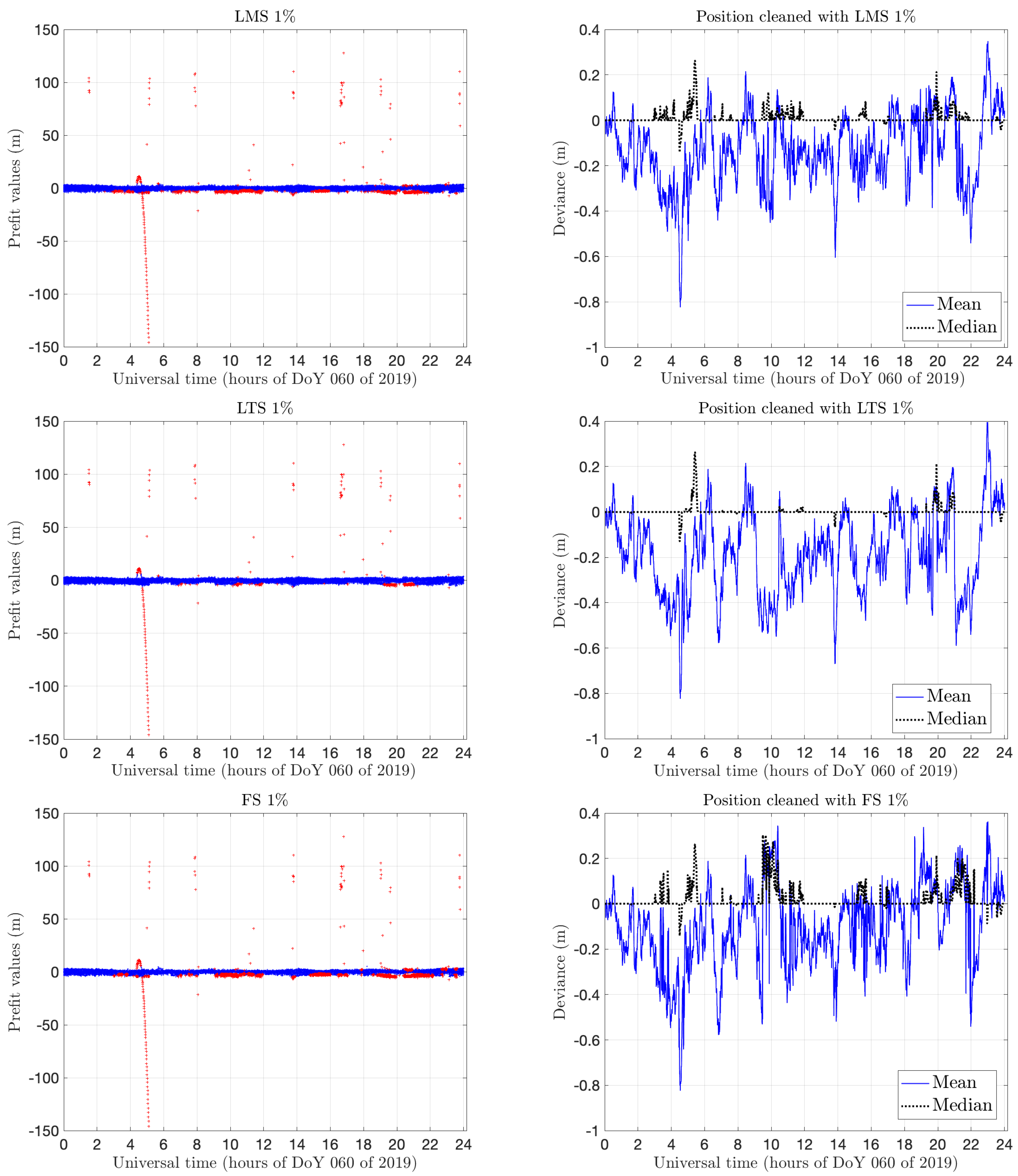
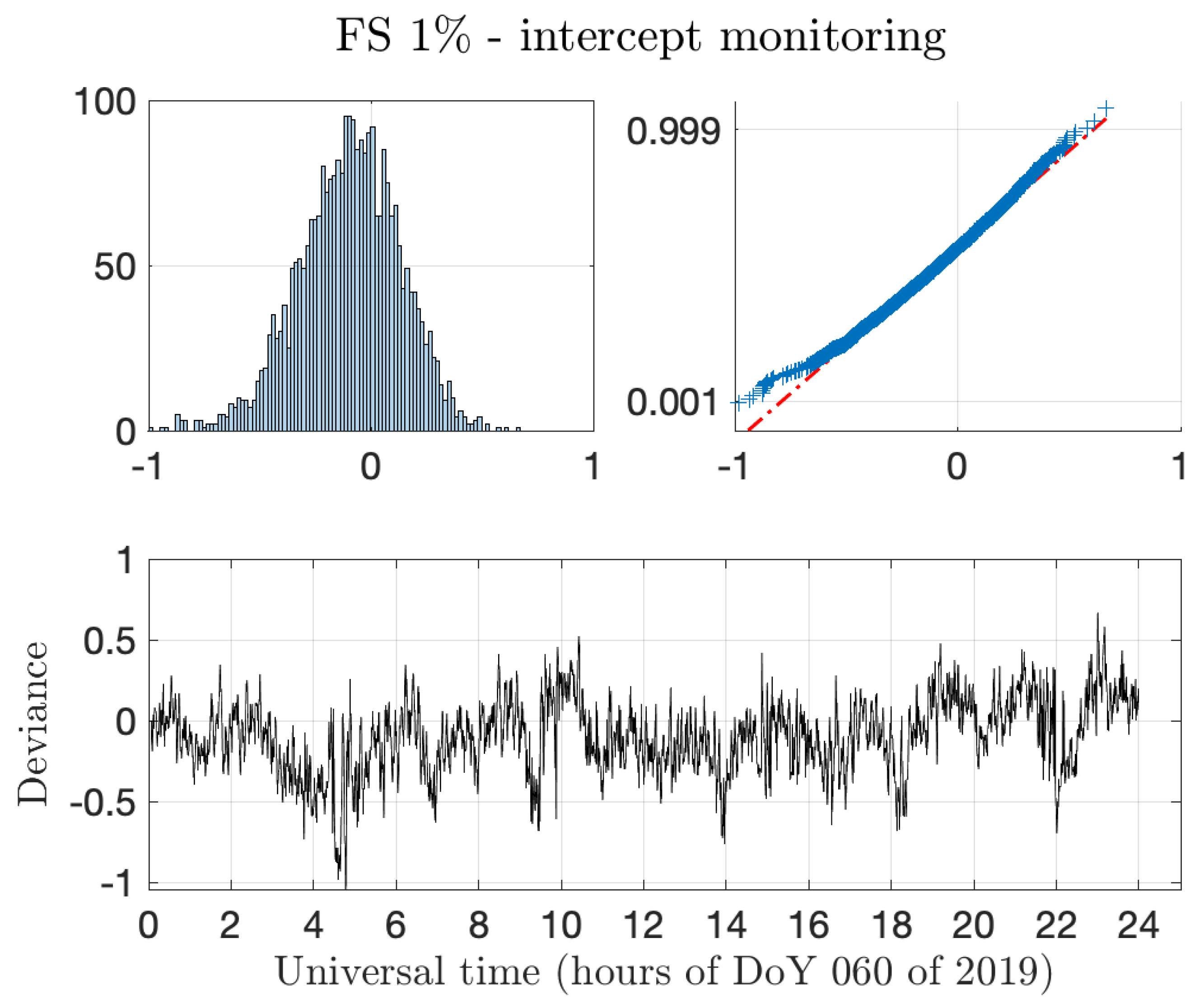
Figure 4 shows the comprehensive results of outlier detection for the defined time window with LMS, LTS and FS and the evolution of mean and median in each case. The plots of mean and median monitoring do not show big differences. This is not surprising since the outliers are similar in the three cases. FS shows ‘more centered’ means and medians, meaning a better selection of outliers, and possibly, a cleaner output. Moreover, the mean shows, in the three cases, a ‘displacement’ towards negative values; a comment on this will be given in Section 4.2 below.

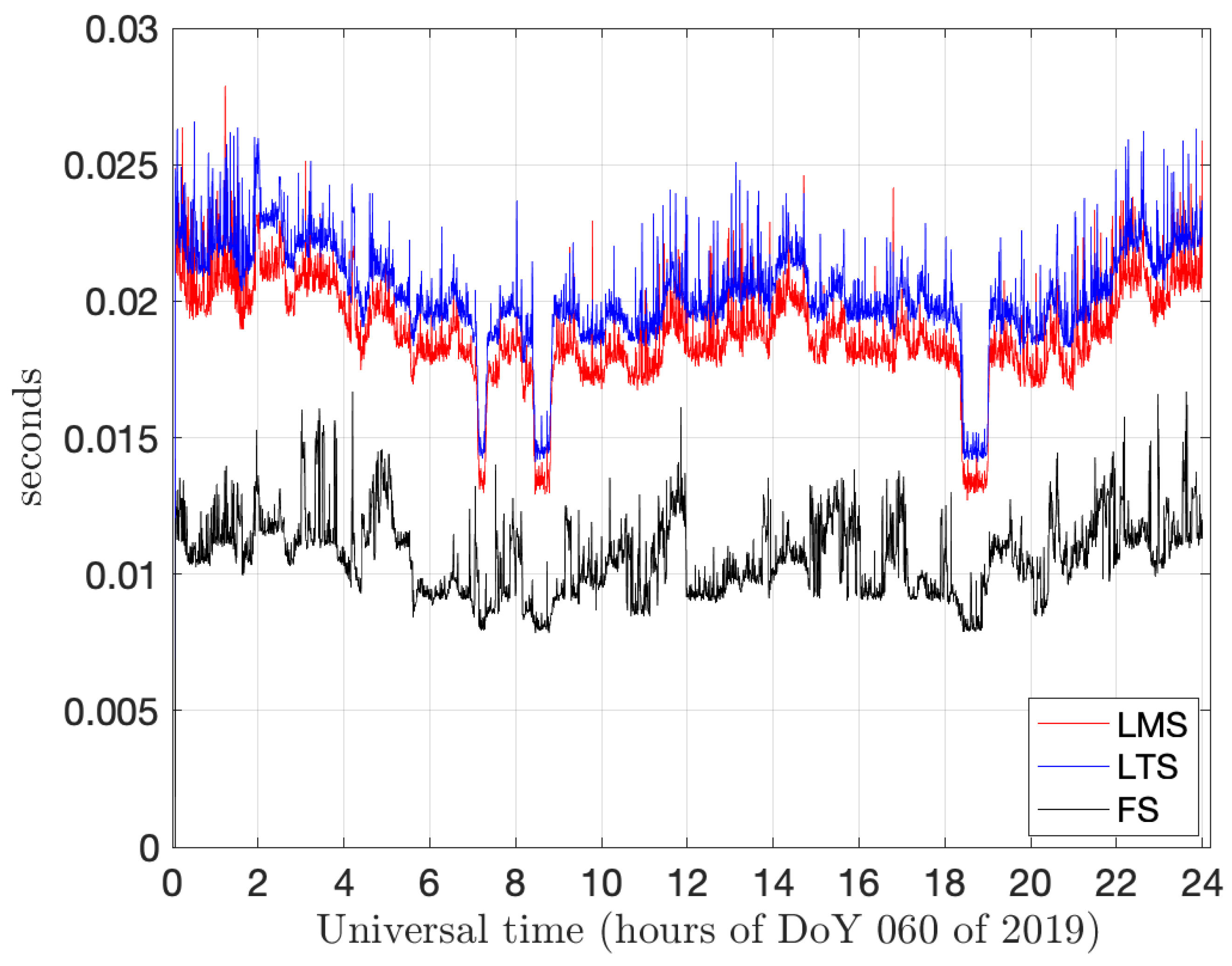
Figure 5 shows the respective computing times for LMS, LTS and FS for each time window lasting 10 epochs on a Quad Core Intel i7, $2.9$ GHz machine.

Table 2. Computing times for the three estimators. The sliding window version of the MATLAB script is applied to the same dataset and with the same MATLAB version.

Estimator	Cumulative (s)	Median of Ten Epochs Windows (ms)
LMS	54.16	18.65
LTS	58.26	20.12
FS	30.56	10.55

reports the respective computing times—cumulative and median—for all 10 epochs windows, and shows a clear computational advantage in using FS in spite of its greater theoretical complexity over LMS and LTS. This computational advantage is due to the efficient implementation of the FS algorithm in FSDA. The three drops of LTS and LMS in computing time are coincident with consecutive epochs containing the lowest number of satellites (i.e., 7) included in the computation. The difference in performance between LMS and LTS on one side and FS in these specific intervals, with a time drop on one hand and almost no change on the other hand, is due to the different computational complexity of the methods, as explained below.

Table 2 and Figure 5 show the respective computing times for the three methods on the HUEG dataset (24 h of measurements sampled every 30 s) and the same time window length (of 10 epochs). The clear advantage of the FS might be surprising, given that the method relies on a process that can iterate as many times as the size of the data sample to be analyzed, say n. Several factors determine the advantage over LMS and LTS. The first one is that LMS and LTS need a minimum number of random samples of size $\lceil n/2\rceil$ selected with computationally intensive ‘sampling without replacement’ methods. This explains why Figure 5 shows a visible drop in computing corresponding to the three intervals where data come from only 7 satellites instead of 9–10 as in the majority of cases.

Instead, the FS is initialized with an LMS/LTS regression estimated on very few data points (those sufficient to fit the regression line, therefore two points as a minimum, in our case) and this is computationally trivial. Then, it progresses with a sequence of order statistics and OLS computations, which are also computationally simple. Finally, FS can start monitoring for potential signals only in the final part of the search, and this additionally reduces its computational burden. As a reference, on the same machine, the computation of the SPP by gLAB with only the default outliers (satellites with a pre-fit residual greater than forty meters and with elevation lower than five degrees) is done, resulting in a median over eleven trials of 1.078 s on the same dataset. In this setting, i.e., the MATLAB-interpreted version of FS, the time overhead for the FS computation in the case of a moving window results in $30.56$ s. However, it is noted that although in its interpreted version (i.e., not compiled), FS processes 24 h of data in half a minute, which enables real-time operations.

4. Results, Discussion and Proposal for Further Work

4.1. Positioning Results

This section illustrates how actual outliers present in the pre-fit residuals deteriorate the PVT estimated within the FILTER module. The coordinates of permanent stations are known with errors at the centimeter level. Then, because the magnitude of the outliers is at the few meters level, we can use the positions of permanent receivers as a reference truth to infer the impact of such outliers in the position estimates.

Figure 6 depicts, at every epoch, the 3D errors of KIR0, computed with the norm of the difference between the XYZ coordinates estimated using the pre-fit residuals and the reference coordinates. The red color depicts the positioning error without taking any action to filter outliers, whereas the blue color shows the errors when outliers are identified and removed following the preliminary analysis with the LMS of Section 2 above. It can be seen how the original 3D errors grow up to 12 m, coincidentally with the time the GPS satellite 32 is observed in Figure 1. Figure 6 and its numerical counterpart

Table 3. Mean, median, 68th and 95th percentiles and RMS of the positioning errors obtained for the two permanent stations, KIR0 and HUEG, applying different outlier detection methods. Note that the ‘NONE’ method only excludes satellites with an elevation lower than 5 degrees.

Station	Outlier Detection Method	3D Positioning Error (m)
		Mean	50%	68%	95%	RMS
KIR0	NONE	2.21	1.61	2.13	6.83	2.93
KIR0	LMS	1.55	1.44	1.76	2.90	1.70
HUEG	NONE	5.23	2.57	3.05	6.00	15.21
HUEG	LMS	2.23	2.15	2.67	3.84	2.41
HUEG	LTS	2.45	2.39	2.84	3.96	2.60
HUEG	FS	2.26	2.18	2.67	3.87	2.44

, show that once these outliers are detected and removed, the 3D error is kept at the level of a few meters, as expected in the typical SPP.

Figure 7 depicts the 3D errors of HUEG, following the same method to produce Figure 6 for KIR0. In this case, the original 3D error obtained with SPP reaches almost 120 m, due to the presence of the outliers previously depicted in Figure 3. In contrast, 3D errors obtained with robust statistics present an accuracy of about one order of magnitude better in terms of RMS, as confirmed in Table 3. There are some discrepancies between the positioning errors obtained by the LTS, LMS and FS methods, which witness an overall good performance of all the three robust estimators and confirm the good trade-off between results and computational efficiency provided by the FS.

4.2. Discussion

Figure 8 is a detail of Figure 7 for small position errors; Figure 9 is a zoom of Figure 8 for the time period between 18 and 23 h. As can be seen in the upper part of the plot, most of the time, robust outlier detection methods improve the 3D position errors of the original SPP obtained from pre-fit residuals with outliers.

However, there are four epochs between $21h00$ and $21h30$, in which the solution, especially when the outliers found with FS are removed, is deteriorated compared to the original one. In order to explain such a result, the bottom plot depicts the geometric dilution of precision (GDOP), which is a measure of how the measurement noise impacts (i.e., dilutes) the positioning accuracy (see, for instance [4,7]).

The GDOP metric evaluates the geometric distribution of the satellites over the sky, only being computed with the elevation and azimuth of the satellites whose measurements determine the position in the FILTER module. The GDOP depends not only on the number of satellites used to compute the coordinates, but also on its distribution in the sky. In this regard, discarding satellites typically increases the GDOP and the positioning error. At $21h15$, it can be seen that the GDOP values for the FS reach four times the GDOP values of the original solution, which uses nine satellites in view with an elevation greater than 5 degrees. The reason is that the FS discards two low-elevation satellites that greatly contribute to the positioning estimation. Fortunately, these high GDOP values are an indication to the user that the coordinates are being estimated with a weak geometry and consequently should be used with caution.

There are a number of measures to mitigate the deterioration in the positioning error. First, one should use a more accurate modeling of the measurements than the one used in SPP, as in [21]. This would, in principle, reduce the dispersion of the pre-fit residuals, easing outlier detection. Second, one should consider the pre-fit residuals obtained from distributions other than the normal one for detecting outliers. Third, the information of the satellite geometry (elevation and azimuth) should be included in the robust methods, since the present exercise has done a blind examination taking into consideration only pre-fit residuals, but not, for instance, their possible correlations. Fourth and finally, the robustness of the Kalman filter itself should be increased, coordinating the effort of the outlier detection in the pre-fit residuals domain and in the final filtering module domain.

Figure 10 shows in detail the behavior of FS during one of the computations described in Section 3 on a time window of 5 min, starting at $20h34$. The horizontal axis represents the size m of the subset used at a given step of the FS process to fit the regression model. The FS process is such that outliers enter the subset ‘towards the end’. The vertical purple lines show the moment when the monitored statistic (minimum deletion residual—$r_{min}(m,n)$—among the observations not yet included in the subset) exceeds the confidence bands at different levels of significance. The FS algorithm checks whether the exceedance from the bands is not spurious (that is, it remains persistently out of the confidence limits in the sense formalized by [22]), identifies its precise position, in addition to the units forming a homogeneous subset, and ultimately those to be declared outliers. Note that the progression of $r_{min}(m,n)$ ($m=45,\dots ,90$ in the example) re-enters in the middle of the confidence bands at the end of the FS: this is the so-called ‘masking effect’ occurring in presence of outliers if all the data fit, such as the case of OLS. In this case, outliers mask each other and one cannot detect them. In a nutshell: OLS provides only $r_{min}(n,n)$, which is excellent if all the n data points are good; LTS/LMS only provide the very robust fit for $r_{min}(\lceil n/2\rceil ,n)$, which is excellent if there are many outliers (up to $\lceil n/2\rceil$); FS mediates between the two extremes by providing a sequence of fits with $r_{min}(m,n)$, $m=m_0,\dots ,n$ and by identifying the optimal subset with $m^{*}$ good units.

Figure 11 gives three views of the intercepts estimated as the moving window of 10 epochs progresses with time. The top panels represent the distribution of the deviations of the estimated values from the desired one, which should be zero. The histogram suggests that the fluctuations observed in the time representation of the bottom panel are rather symmetrical. On the other hand, the view provided by the normal probability plot on the top right, which compares the empirical distribution of the intercept estimates to the normal, indicates the extent to which the left and right tails deviating from the normal differ. This suggests the presence of a small systematic bias in the way positions are received.

This possibility is corroborated by the experiments performed with the robust estimators in Section 3 above, which raise some questions. While considering the plots of the mean and median in Figure 4, we already remarked that the mean looks ‘biased’ by the negative outliers. These problematic data points correspond to pre-fit residuals of low-elevation satellites, when the receiver is rising or setting above the local horizon. In such circumstances, the SPP cannot accurately model propagation delays (e.g., at troposphere and at ionosphere). Moreover, the noise of the measurements increases due to multipath (i.e., reflections of the GNSS signal on the ground or metallic structures). A more precise modeling of the measurements to the one used in SPP (see for instance, [21]) would, in principle, reduce the dispersion of the pre-fit residuals. This would probably ease the detection of outliers, although new borderline cases (i.e., on the limit to be considered as outliers) would appear.

4.3. Further Work

There have been several attempts at using robust statistics techniques in GNSS positioning, as mentioned in Section 1. Our study relies on the specific gLAB module dealing with the analysis of pre-fit data where the difference between the modeled and computed range, the pre-fit residuals as in Table 1, is meaningful. In this case, we showed that outlier detection via FS gives an advantage both in terms of number of true outliers found and computational efficiency with respect to LMS and LTS. This advantage can be further improved by considering all the information available, like elevation, geometric dilution of precision and correlation between epochs and satellites. Moreover, it is quite natural to wonder whether robust methods can be used in other modules of gLAB, namely the PREPROCESSING and the FILTER modules, in order to distribute the effort of the outlier detection and ultimately improve the quality of SPP and possibly, the precise point positioning (PPP) [23]. Another research direction would be to apply the FSDA functions to actual data collected by a moving receiver, as for instance autonomous drones [24]. In this regard, we remark that the current implementation of the Kalman filter in the FILTER module is the classical one, hence it is not robust. This kind of analysis will probably involve the use of robust time series, a topic which will be the main subject for the continuation of the present work. By aiming at ‘real-time’ applications, we note that the translation in C language of the FSDA functions is a task currently in progress that should improve the time overhead in the use of robust methods remarked at the end of Section 3. A subsequent analysis of the flow of data in the C code could lead to a parallel implementation of the basic routines and a subsequent translation in an appropriate high-level language for hardware design.

5. Conclusions

The position solution computed by means of satellite measurements strongly depends on how the data are processed. The present study is concerned with thesStandard point positioning employed in the mass-market receivers, and exploits the pre-fit residuals of datasets referred to the position of permanent receivers. The normal flow of data through software packages for GNSS processing is considered by using gLAB as a reference. In the main steps of this flow of data, the treatment of pre-fit residuals comes immediately before the final FILTER module that outputs the computed coordinates. The experiments done in this specific case show positive results and pave the way for a number of further improvements and studies, as indicated in Section 4.2 and Section 4.3, on the potential use of robust statistics for GNSS positioning. These improvements are in line with a present trend in the use of robust statistics for GNSS positioning, as briefly mentioned in Section 1. The element of novelty added in this work is in the use of forward search techniques and in the exploitation of pre-fit residuals. The results on positioning presented in Section 4.1 prove that the robust statistical methods used correctly identify the actual outliers present in the GNSS measurements, contributing in this way to the improvement of accuracy and the reliability of satellite-based positioning services. Among the points listed in Section 4.2 for further reflection, it was remarked once more that users shall, as in any other positioning method, observe the GDOP metric to decide whether the coordinates are being estimated with a weak geometry, especially in the event of discarding multiple satellites.