Abstract
This paper presents a comparative analysis of performance for several antenna prototypes using a screen-printing process. This analysis was performed using various bow-tie antenna configurations, including single-band and multi-band antennas with linear or circular polarization over multiple operating frequency ranges. For antenna implementations, three different conductive inks and two resolutions of screen masks were tested. The performance of the fabricated prototypes has then been compared to the copper laser-etched antennas. This study revealed that with the proper selection of ink thinness, screen-printed bow-tie antennas achieve similar performances to copper laser-etched bow-tie antennas up to 6 GHz, even for linearly polarized and circularly polarized antennas. However, the printing resolution should be improved by reducing the ink thickness for bow-tie antennas at higher operating frequencies. The measurement results show a successful agreement after improving the printing resolution of the fabricated 5.8 GHz and 15 GHz bi-band bow-tie antennas.
1. Introduction
The increasing demand for connectivity has spurred the widespread adoption of IoT technologies in both research and industries. With 43 billion devices connected in 2023, projections indicate that this number will surpass 50 billion by 2030 [1,2]. Such a surge in connected devices requires the mass production of low-profile and low-cost antennas.
To cater to the demand for ultra-low-cost connected devices, manufacturing processes such as additive manufacturing production offer significant cost reductions thanks to the economies of scale. These techniques enable the production of several electronic components on large surfaces while minimizing the use of conductive materials to the strict necessary. Moreover, some mechanical properties such as resistance to vibrations or deformations could be beneficial for flexible electronics. Although various additive printing techniques on flexible substrates are available for easy prototyping [3], most of them suffer from slow production speeds and require conductive inks with very low viscosity. Moreover, flexography printing, as highlighted by [4], is expensive to implement despite its achieving outstanding performance.
The comparison of various printing processes in Table 1, shows that screen printing provides the best trade-off between line spatial resolution, printing speed, and line thickness. Furthermore, screen-printing emerges as one of the most promising candidates for low-cost antenna mass production since it enables the deposition of thick ink layers on various surfaces.

Table 1.
Comparison of different printing methods.
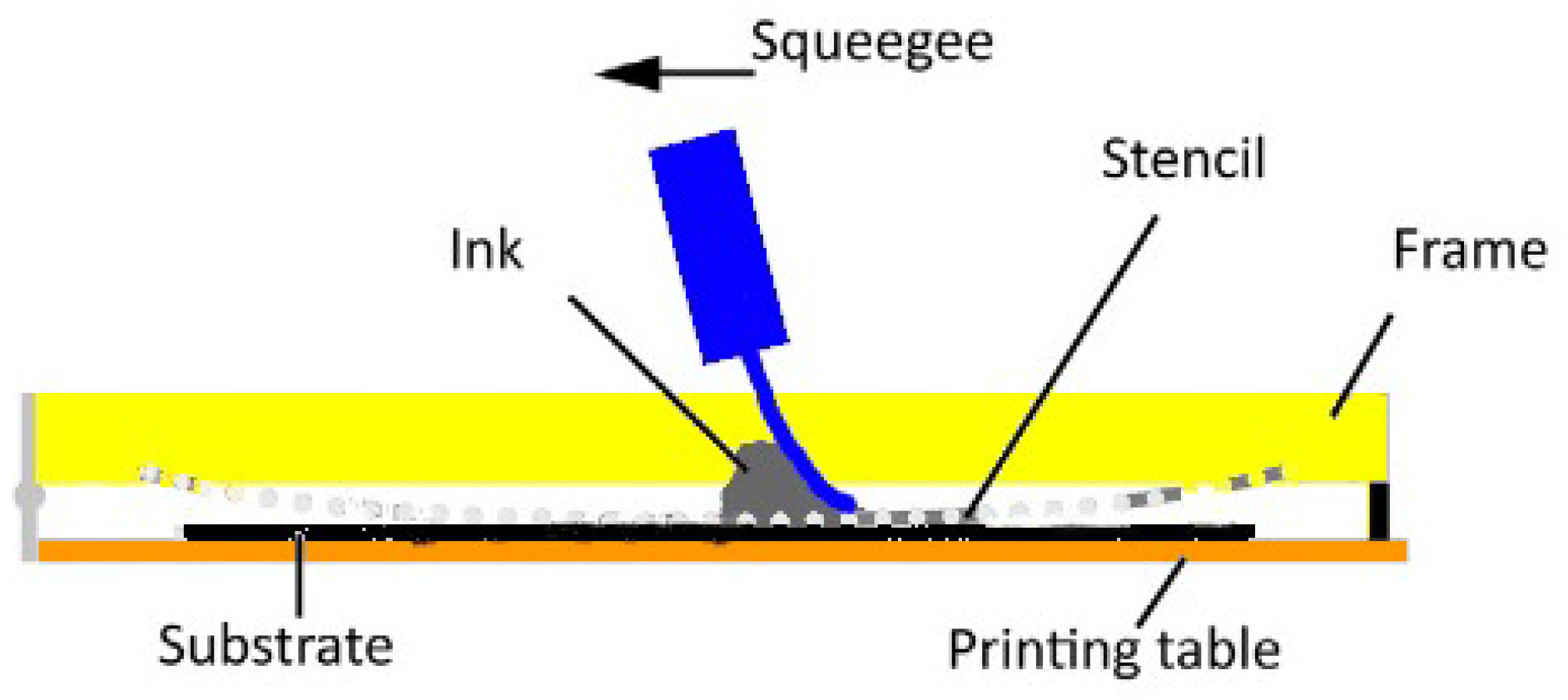
In the screen printing process, ink is spread on a stencil by a squeegee (see Figure 1). Thus, when the stencil is transparent, the ink is deposited on the substrate. The process requires the precise management of stencil mesh and squeegee properties, as well as production techniques. It may also require tightly controlled parameters during printing. Furthermore, ink transfer is mainly influenced by the screen mesh, squeegee speed, and pressure on the screen. The thickness and accuracy of the printed layer are affected by the ink’s rheological properties. It should be noted that thicker ink deposition involves lower resolution.

Figure 1.
Schematic of the screen printing process.
Currently, industrial screen printing resolution can achieve line widths as small as . However, with ongoing improvements in processes printing line widths as small as could be possible. The feasibility of screen-printed antennas is already established, as multiple articles relate to screen-printed antennas realized on textile materials or flexible substrates, as reported in [5,6,7,8]. Some authors [9,10,11,12,13] investigated silver paste to print RFID antennas or compared inkjet and screen-printed RFID antennas in the megahertz frequency range. Other studies focus on the stability of matching of washable antennas [14]. However, they investigate process improvements, such as [15,16], which proposes the use of graphene-based or nanotube inks to print textile antennas or harvesting devices. Although in the works stated above, designs and performances have been detailed, the information on the impact of the screen printing process on the performances of the antennas were not revealed. They suggest the feasibility of screen-printed antennas and focus on the usability and performances of the antenna topology. However, only a few provide details on the printing process. This paper investigates the effects of ink printing imperfections on the performances and cost of screen-printing antennas over the gigahertz frequency range. Those imperfections mainly include low conductivity of the ink, the thickness of the printed layer, low printing resolution in the gigahertz frequency range or misprinting uses. For the performance investigation of the screen printing process, a simple antenna topology has been selected. Antennas such as PIFA, IFA, or meandered dipoles [17,18,19,20] are characterized by their design complexity and sensitivity to fabrication tolerances, making failure analysis more complex. This is mainly due to the implementation inaccuracy of metallized via-holes, compared to a standard PCB process. We then selected bow-tie antennas with different configurations due to their low complexity design [21] as an alternative for analysis validation. In this perspective, the impact of resolution, mismatch between top and bottom layers, and ink conductivity has been investigated over the and ISM bands. The performance analysis includes simple bow-tie antennas and circularly polarized bow-tie (CP bow-tie antennas), where each antenna has been designed to cover the range and the ) range ( and ISM bands).
In addition, a double-band bow-tie antenna ( and ) is presented to test the limitations of the printing process at higher frequencies. To investigate the conductivity effects and geometrical imperfections of printed pattern impacts on antenna behavior, each antenna has been printed with three different silver inks and has also been realized using a standard laser etching technique. The paper is organized as follows: The second section of the paper deals with the employed ink, the limitations induced by the parameters of the screen printing process, and the optimization of feeding lines used to feed antennas. The third section of the article is devoted to the designed antennas to test the process limitations. The fourth one gives the measurement results and an upgrade of the printing process to increase matching between simulations and measurements. The paper ends with the conclusion on the impact of screen-printing technology for antenna fabrication with an analysis of the impact of ink conductivity and printing accuracy on antenna performances in the gigahertz frequency range.
2. Substrate, Ink, and Feeding Technique
This section depicts various properties of the ink, printing parameters, and substrate selection. These choices involve some rules for antenna design, including minimum line width, spacing between adjacent lines, and feeding techniques. The screen printing prototyping uses a commercial screen printing machine. To improve cost-effectiveness, only textile stencils were utilized to print all the designed antennas.
2.1. Substrates Selection
The substrate plays a key role in antenna performance. It must have low-loss characteristics and be compatible with the physicochemical properties of the selected inks. Substrate selection is a key factor in ensuring good compatibility with inks, particularly with regard to the substrate’s physical and chemical properties. In this section, we expose the essential properties that promote this compatibility. For instance, in the case of inkjet or screen printing with metallic inks, such as silver ink, the substrate must have a microporous receiving layer, either by plasma etching to create nanometric roughness, or by depositing a porous low dielectric such as a fluoropolymer or polystyrene, which enables better adhesion and avoids excessive ink diffusion [22,23]. The characteristics of silver inkjet printing were intensively investigated with control of surface energy, which is why the choice of substrate can greatly affect the quality of the print and consequently the electrical performance of the deposited silver layer. In this study, the Kapton was treated with an oxygen-free plansma to create the micro-pored layer without degradation of the electrical properties of the kapton [24]. For the screen printing process, a Kapton substrate with a thickness of () was chosen. As the antennas were also fabricated using laser etching on the copper metalized substrate, a substrate with identical electromagnetic properties was selected. Hence, a TACONIC RF-35 substrate was chosen for copper-etched antennas. This allows for comparison between the two methods of antenna fabrication, enabling the investigation of the effects of screen printing imperfections through measurement comparisons.
2.2. Ink Selection
To investigate the influence of ink conductivity on the overall performance of the antenna, three different silver inks were employed. Table 2 provides a summary of the properties of these inks, including the penetration depth length (), which is computed using Equation (1).
Table 2.
Properties of different silver inks.
The choice of ink thickness is significantly constrained by the geometrical printing accuracy, which should be thinner than the smallest element of the antenna. Thus, selecting the layer thickness involves a trade-off between cost and resolution. It is noteworthy that for a given mesh density of the stencil, the printed pattern’s resolution increases with decreasing printed layer thickness. Since most of the current is concentrated in the skin length of the conductor at high frequencies, the ink thickness is set to be close to the skin depth () for each type of ink (see Table 2).
With such ink thickness, the anticipated resolution is around for ink strips and for slots formed on ink strips. This resolution should be suitable for printing bow-tie antennas operating at both operating frequencies, and . To quantify the impact of conductivity losses and printing imperfections, all antennas were fabricated on a Taconic RF-35 substrate using laser etching techniques. It features two thick copper layers.
2.3. Antenna Feeding Technique
Using an appropriate antenna feeding method is essential, particularly at multi-gigahertz frequencies. Various feeding solutions on flexible substrates can be employed for this purpose. For a comprehensive characterization of the designed antennas to maintain reproducibility and efficiency, a Southwest Microwave End Launch Connector along with a micro-strip line are implemented. The designed micro-strip lines consist of a signal strip printed on the top face of the substrate, with a ground plane printed on the bottom face. To improve cost-effectiveness, the ground plane width is minimized to reduce ink consumption. It should be noted that there is a trade-off between minimizing ink amount and minimizing losses on the feeding line when determining the breadth of the ground plane.
3. Antenna Design
The following sections outline the design method of the proposed antenna configurations and their performances. Additionally, for all designs, a reference “copper antenna” with a thick copper metal layer has been simulated. These etched copper antennas are named “Cu” in all graphs. In addition, all simulations have been performed with the 3D full wave ANSYS HFSS 2020 R2.
3.1. Single-Band Bow-Tie Antennas
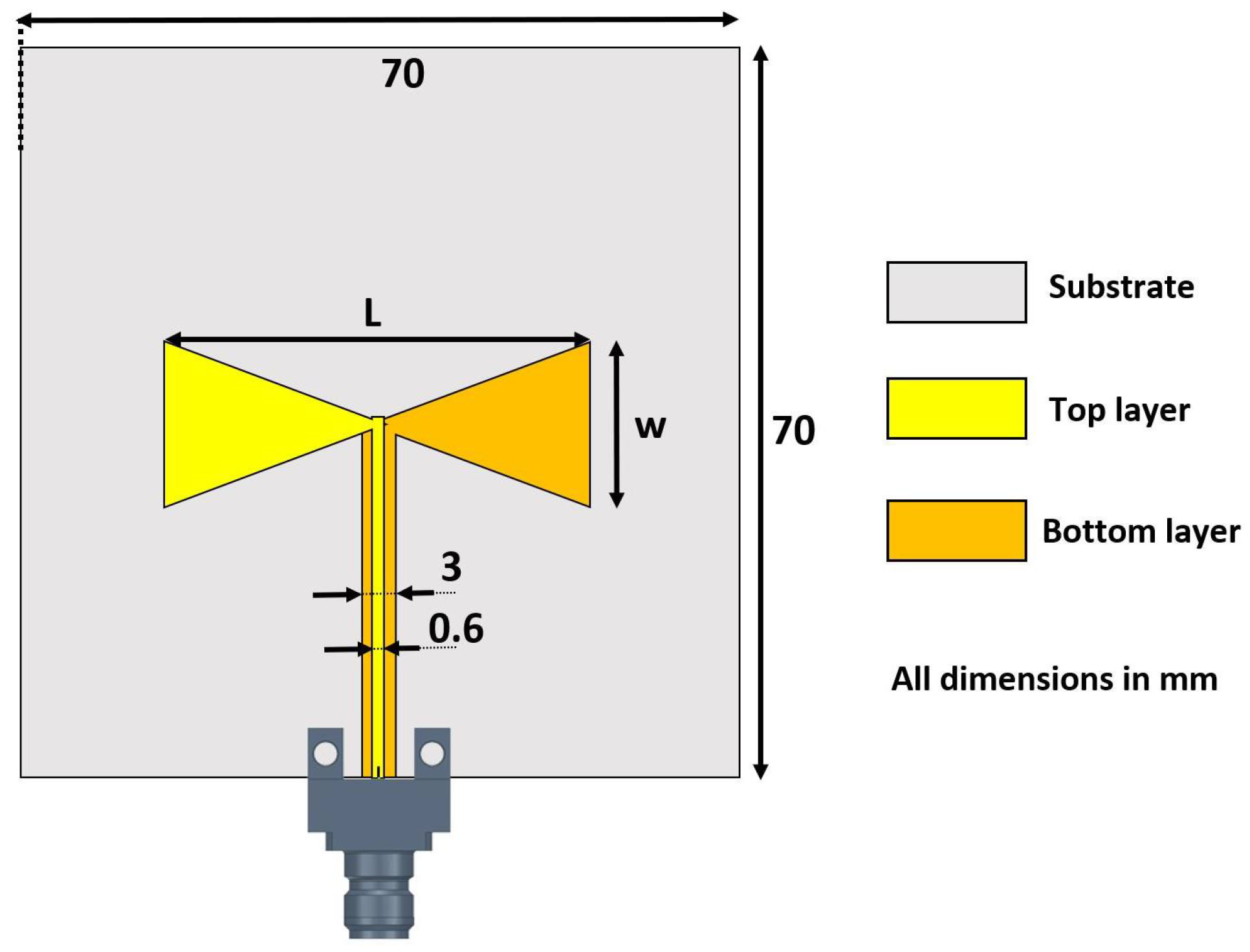
The first designed antennas for screen-printing process performance analysis are single-band and linearly polarized. They operate over to and ( and ISM bands). Figure 2 shows the design of a typical bow-tie antenna to be screen-printed.

Figure 2.
Top view of a typical bow-tie antenna.
The antenna includes two symmetric triangular metallic shapes forming arms. Its length L, as shown in Figure 2, determines the resonant frequency, while its width W enables an adjustment of the impedance matching. In our configuration, the left arm is placed on the top layer, whereas the right one is set on the bottom layer (refer to Figure 2). The characteristic impedance of the 50 microstrip line whose geometric parameters are depicted in Figure 2 is slightly dependent on frequency. The signal strip is connected to the top arm, while the ground strip is related to the bottom arm of the antenna. In this way, two antennas were designed. Table 3 presents the geometrical parameters of the bow-tie antennas. For each antenna, the key performance indicators include the frequency band meeting a satisfactory impedance matching () and the broadside direction realized gain.
Table 3.
Geometrical parameters of linearly polarized bow-tie antennas.
3.1.1. Bow-Tie Antennas
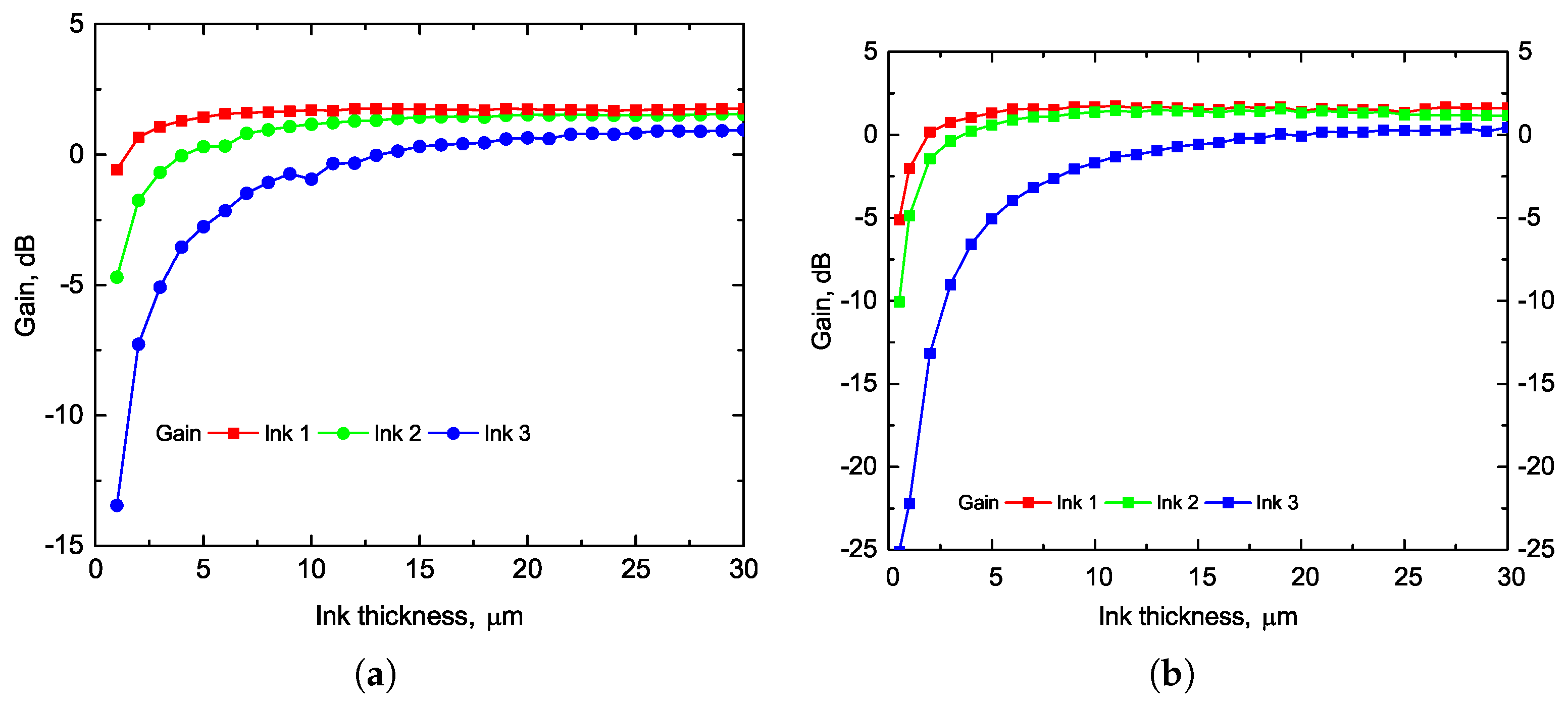
The antenna’s design was simulated with three different ink parameters. To indentify a suitable thickness, the antenna was simulated by varying the ink thickness. The impact of the ink layer thickness on the realized gain at was then plotted in Figure 3a and at in Figure 3b. This allowed for an assessment of the sensitivity of the antenna’s performance to changes in ink thickness.

Figure 3.
Influence of ink layer thickness on the gain of the bow-tie antenna (a) at and (b) at .
Simulation results show that a careful choice of ink thickness enables a imilar gain () for Ink 1 and 2. However, for Ink 3 the maximum realized gain is slightly lower ().
The antenna’s performance over the to frequency range was investigated through varying ink thickness and conductivity. The results plotted in Figure 4 show that the conductivity of the ink has a minimal impact on the antenna’s performances, if the ink thickness is appropriately set for each ink. The simulated gain ranges from (with Ink 3) to (with a copper-etched antenna). Notably, antennas made with Ink 1, Ink 2, and copper display a nearly similar simulated broadside peak gains. Furthermore, the antenna demonstrates a best impedance matching from to .

Figure 4.
Simulated (a) and gain (b) of the bow-tie antenna as a function of frequency.
3.1.2. Bow-Tie Antenna
To assess the impact of ink thickness and its associated resolution at higher frequencies, bow-tie antennas operating over ISM frequency band have also been designed.
The antenna’s performance was simulated, incorporating the parameters of three different inks, including conductivity and layer thickness. All simulation results are depicted in Figure 5. The simulations show that the conductivity of the ink has a minimal impact on the antenna’s performance metrics. The realized gain ranges from (Ink 3) to (Ink 1). The simulated bandwidth in which the antenna is matched spans from . It effectively covers the ISM band. Additionally, utilizing ink instead of etched copper results in a peak gain reduction of .
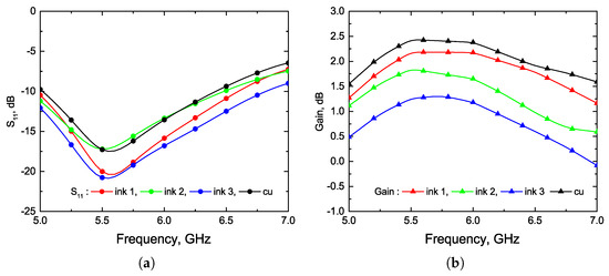
Figure 5.
Simulated (a) and gain (b) of the bow-tie antenna as a function of frequency.
3.2. Circularly Polarized Antenna
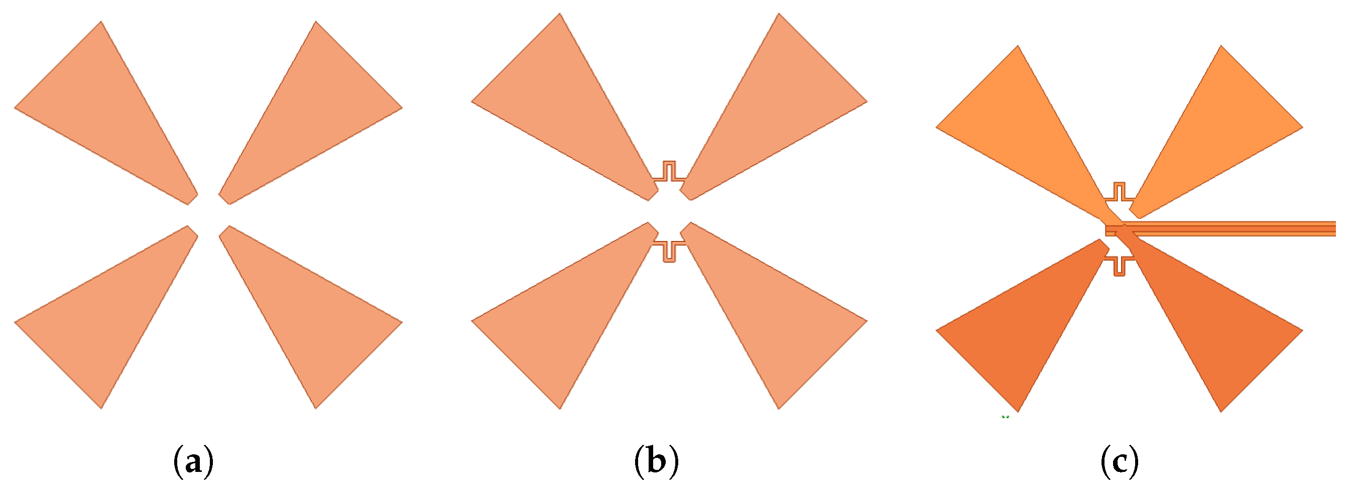
The circularly polarized bow-tie antenna is designed according to the methodology proposed in [25]. As depicted in Figure 6, it involves the use of two cross-fitted bow-tie antennas (see Figure 6a) connected by two phase shifters (see Figure 6b). Subsequently, the antenna is divided into two parts, with the first part printed on the bottom layer and the second part on the top layer. Finally, the antenna is fed by a 50 micro-strip line with an end launch southwest connector as shown in Figure 6c.

Figure 6.
Design steps for circularly polarized bow-tie. (a) Initial design (b) Initial design with a phase-shifter (c) Final design with a feeding line.
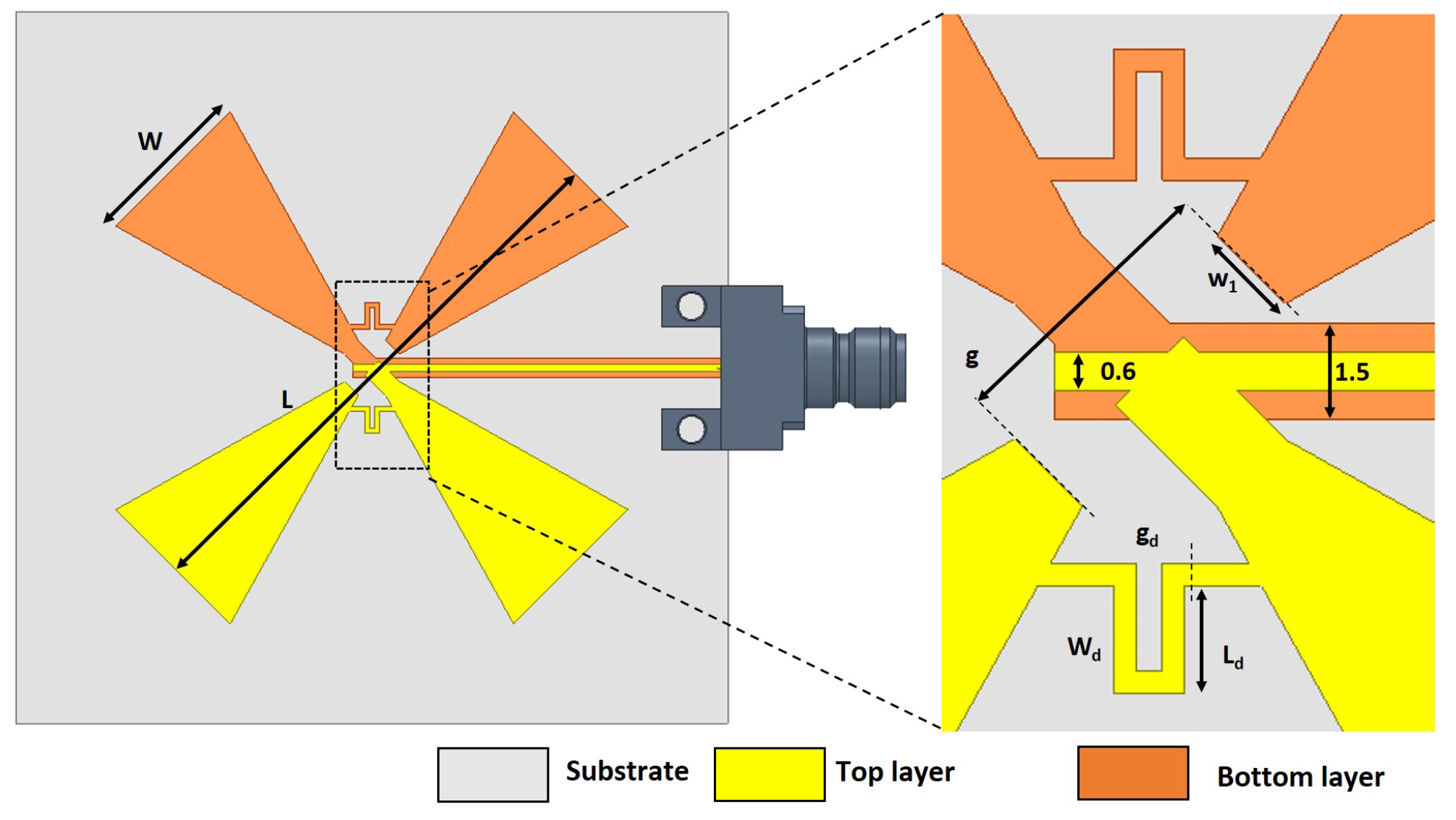
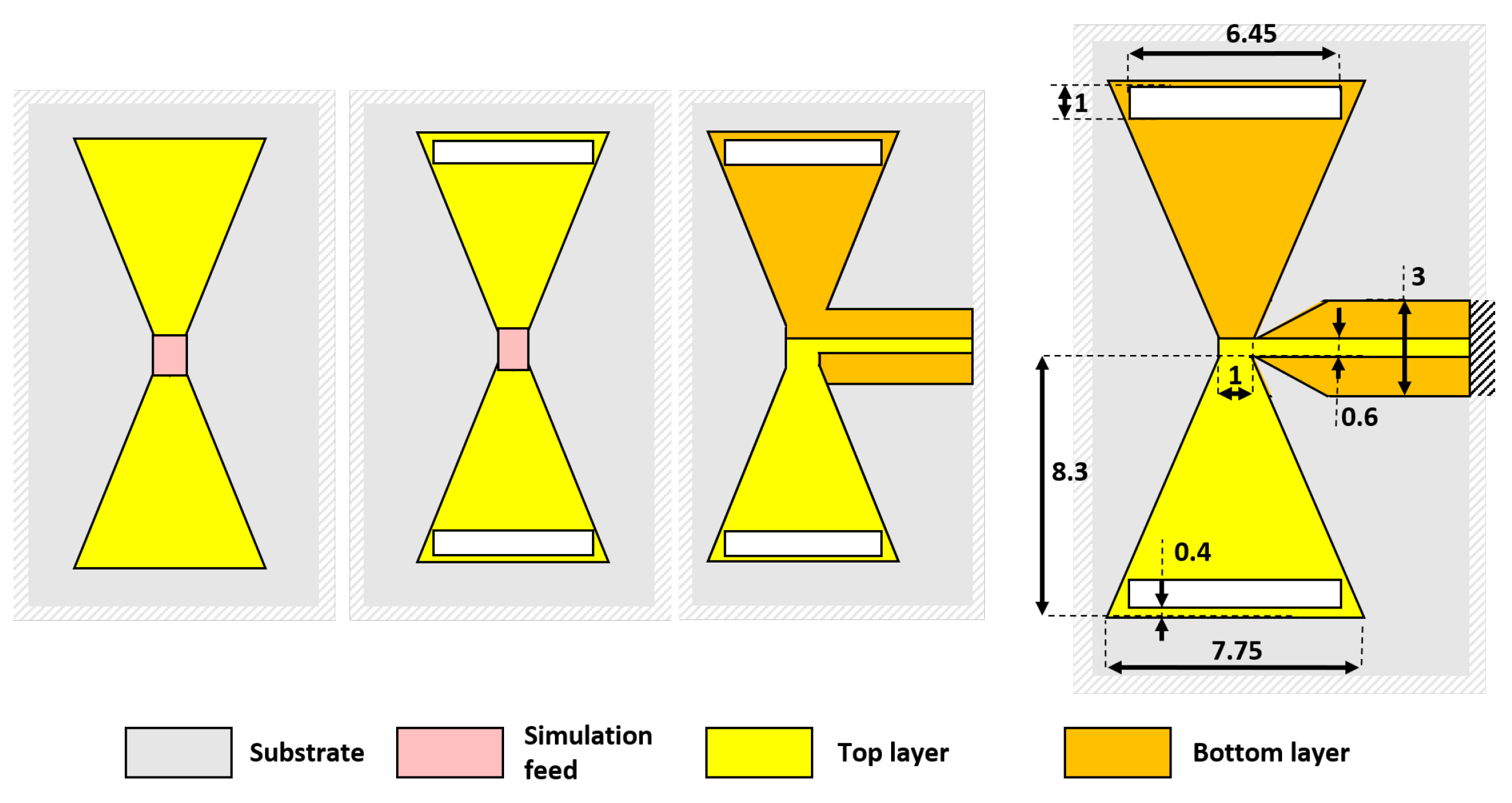
Based on this design approach, two antennas have been developed to operate over the ISM band and ISM band. Figure 7 shows the top view of the antenna along with the definitions of its geometrical parameters. These parameters are summarized in Table 4 with their optimized values. Both antennas have identical dimensions of 7 × 7 .

Figure 7.
Top view of a circularly polarized antenna and its geometrical parameters.
Table 4.
Geometrical parameters of circularly polarized bow-tie antennas (all dimensions in mm).
For circularly polarized (CP) antennas, the key performance indicators include maximum gain, matching bandwidth, and the frequency range, where the axial ratio is below [26].
3.2.1. CP Bow-Tie Antenna
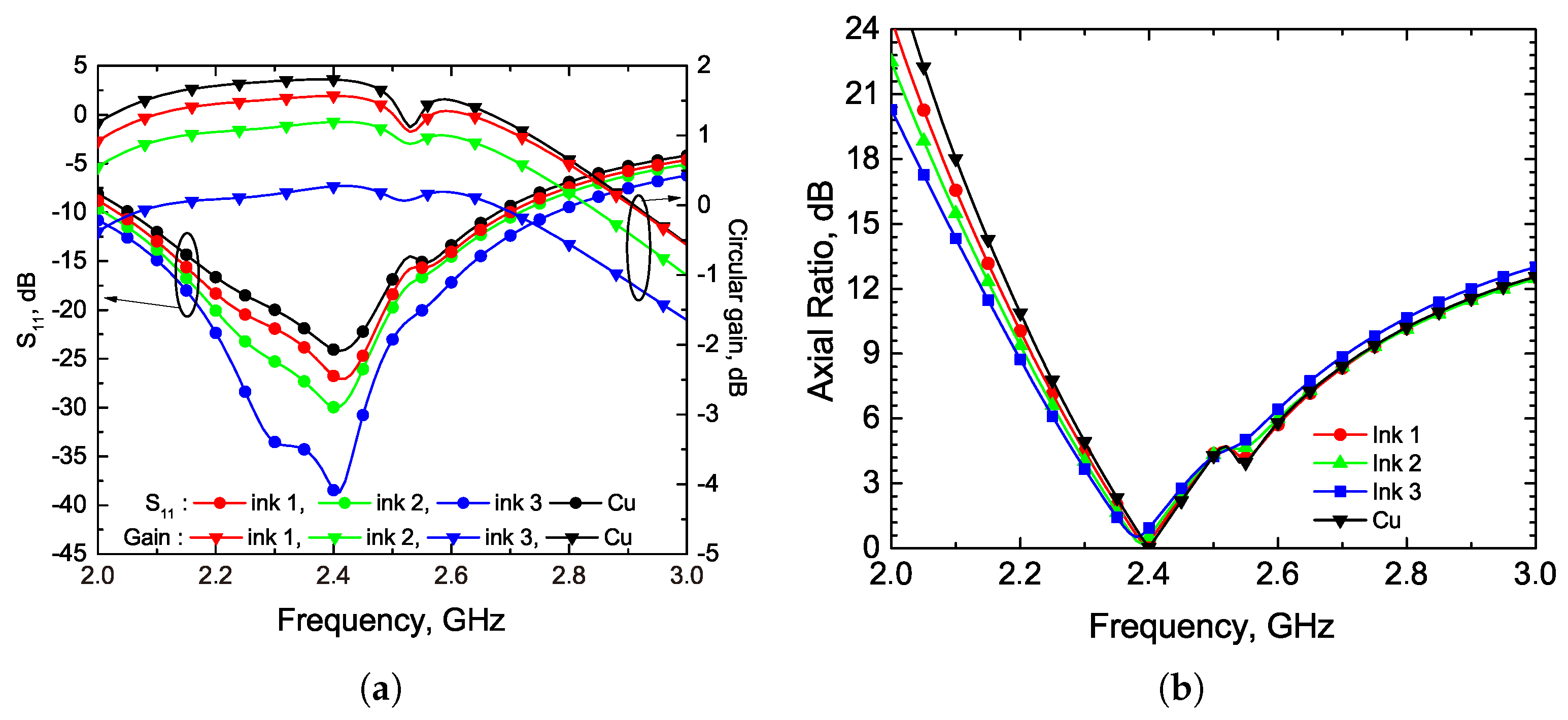
According to the design methodology outlined in [25], a circularly polarized antenna operating at has been successfully designed. Simulations were performed to take into account the effects of the end-launch connector used during measurements, as well as the influence of the thickness and conductivity of each ink used for antenna printing. Additionally, a reference “copper antenna” was simulated for comparison purposes.
Figure 8 presents the simulation results for the designed circularly polarized antenna. It demonstrates a matching bandwidth ranging from (see Figure 8a), along with axial ratio bandwidth covering from (see Figure 8b). Notably, the axial ratio remains unaffected by variations in ink conductivity.

Figure 8.
Simulated , gain (a) and axial ratio (b) of the CP bow-tie antenna.
Within the matched frequency band, the circular gain ranges between 1 and . Since the axial ratio is primarily determined by the antenna’s geometry, the axial ratio is the same for the three inks. Similarly to linearly polarized antennas, the gain shows minimal dependence to ink conductivity when the ink thickness is carefully selected.
3.2.2. Circularly Polarized Bow-Tie Antenna
Following the proposed rules, a bow-tie circularly polarized antenna has been designed.
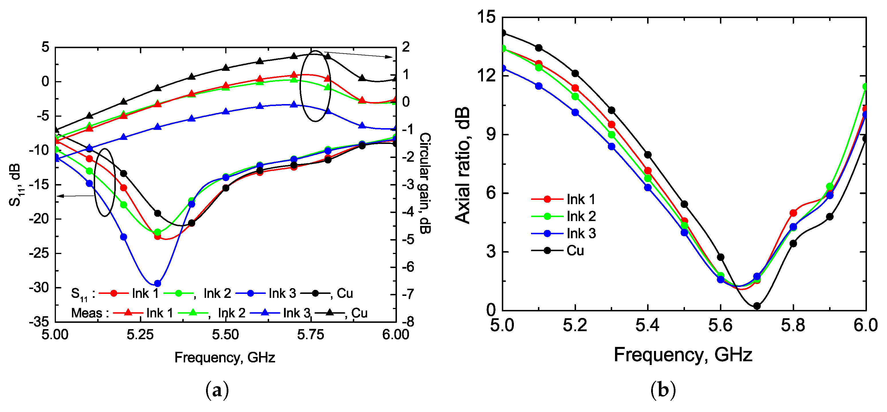
Figure 9a illustrates the parameter and the circular gain. It depicts a realized gain ranging from within the frequency band where the antenna is matched (i.e., from ). The axial ratio, plotted in Figure 9b, follows the typical pattern where the frequency band exhibiting circularly polarized radiation is narrower than the matched frequency band, spanning from to .

Figure 9.
Simulated , gain (a) and axial ratio (b) of the of the circular bow-tie antenna for Ink 1 to 3 and copper.
These results demonstrate that the ink conductivity of the ink layer is sufficient as the antenna exhibits satisfactory performance within the desired frequency range.
3.3. Bi-Band Bow-Tie Antenna
In order to assess the selected ink parameters at higher frequency (conductivity, thickness) and their associated printing accuracy, a bi-band bow-tie antenna was developed. Figure 10 outlines the different steps involved in the design process. The initial step involves designing a single-band antenna in the lowest band of interest. In the second step, one slot is added at the end of each arm of the bow-tie. The second resonant frequency was determined by the length and position of these slots.

Figure 10.
Design steps of the bi-band bow-tie antenna.
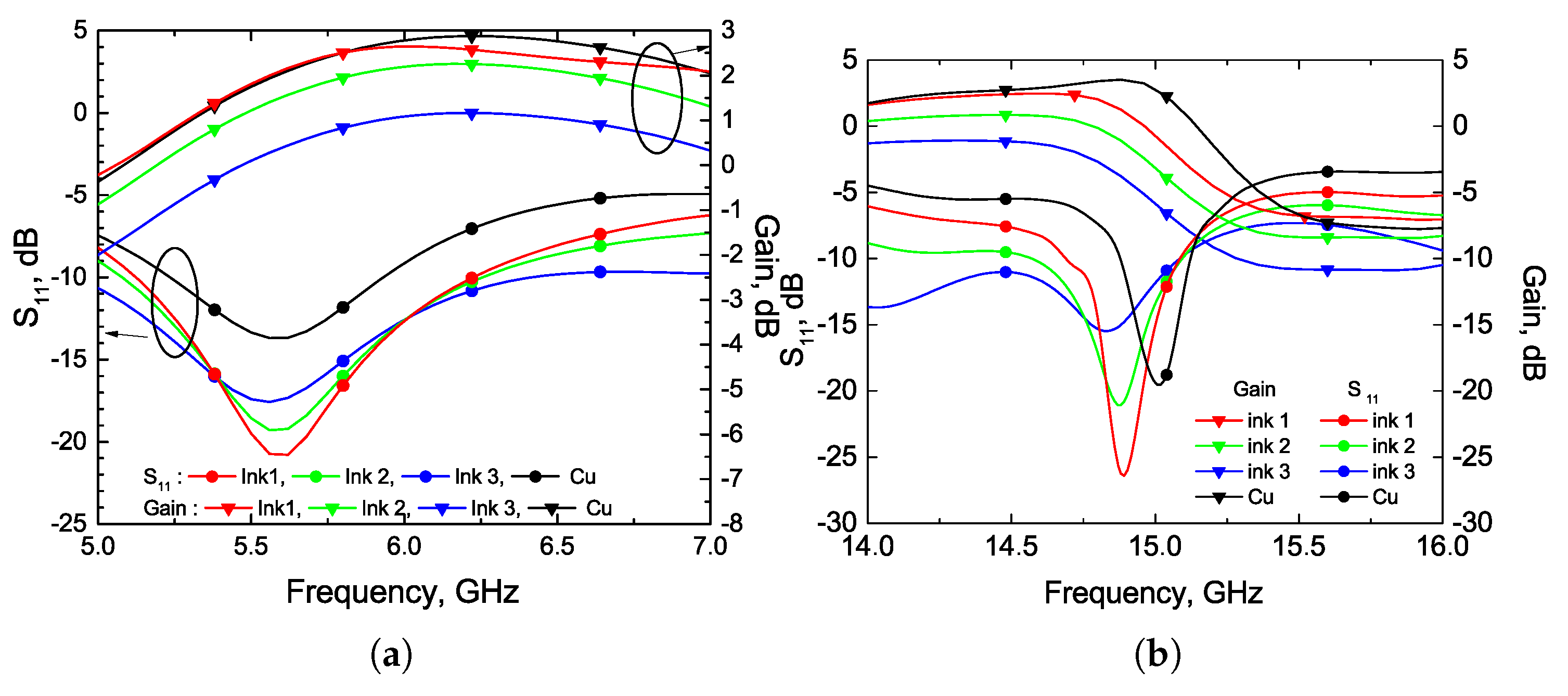
Finally, a 50 micro-strip line as a feeding line is added. The ground plane is tapered to avoid influencing the antenna performance. Using the established design guidelines, a printed antenna is designed and simulated with the properties of the three different inks. The results depicted in Figure 11a include results for an “etched copper” antenna for comparison.
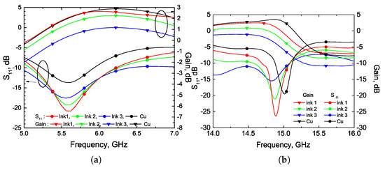
Figure 11.
Simulated impedance matching and gain as a function of frequency of the bi-band bow-tie antenna (a): lowest band (b): highest band.
Similarly to the single-band bow-tie antenna, the simulated results indicate that different inks minimally impact the antenna gain at across the three chosen thicknesses. In the main direction, the gain ranges from and .
Simulation results for the highest band are presented in Figure 11b. In the azimuth 0, the gain ranges from to for the different inks. It is worth noting that the slot’s width is about , the length of the slot is , and its position from the end of the antenna arm is . All these dimensions significantly influence both the peak gain value and the frequency at which the peak gain occurs in both antenna frequency bands. Therefore, this antenna is suitable for a final test of the set of the select screen printing parameters.
4. Measurements and Discussion
In this section, measurements of the conductivity and thickness of the ink layers are exposed, alongside with measurements of the designed antennas. Antenna measurements were performed using the same test bench, in a 5 × 3 × 2.5 anechoic chamber, with an RF spin QRH20E dual-polarized antenna [27], and a ZVA 24 Rhode and Schwartz network vector analyzer (VNA). It is important to note that the antenna measurement error on the gain does not exceed ±0.6 dB.
Matching was measured through a Rhode and Schwartz ZVA 24 analyzer, with the antenna connected to the VNA via a southwest-end launch DC- connector. Measurements of the linear gain were performed using the Friis formula-based technique. To perform measurements of circularly polarized antennas, a linear polarized antenna was rotated in the plane of polarization. For each position of the measuring antenna, the linear gain was measured. The axial ratio as well as circular gain were computed from the measurements [26]. All gain and axial ratio measurements were conducted at the 0 azimuth and 0 elevation direction of the antenna.
4.1. Conductivity and Ink Profile
The conductivity of the ink and the thickness of the printed layers were characterized for each ink. For each ink, the resistance value of a given pattern and the metallization thickness has been measured using, respectively, the four-terminal sensing (4T sensing) technique and a mechanical profilometer. Then, the conductivities of different inks value have been deduced.
The measurements show that for a thick strip line printed with Ink 1, a variation of in thickness was observed. For Ink 2, the variations were more significant, a variation of was observed for a thick strip line, while Ink 3 showed a normal profile; for a strip line with a thickness of , it revealed a profile shaped like a dome. Table 5 summarizes the measured geometrical data and the measured conductivity of the printed layers.
Table 5.
Summary of the measured properties of different silver inks.
Good printing accuracy is achieved according to the measured data and the profiles of the strip lines. The conductivity values are also close to the expected values, confirming the reliability of the fabrication process.
To assess the overall performance of the antennas, we evaluated whether these screen-printing imperfections impact the antenna performance. These imperfections could lead to a gain reduction compared to the expected values, without a significant shift in the operating frequencies. However, imperfections in the geometry of the antennas results in frequency shifts. Measuring the antennas yields important information about how much these influences affect antenna performance.
4.2. Linearly Polarized Bow-Tie
In this section, measurements of linearly polarized bow-tie antennas are presented. Each antenna was printed using the three different inks described earlier. These measurements give insightful information on how the ink’s characteristics affect the antenna performances.
4.2.1. Bow-Tie Antenna
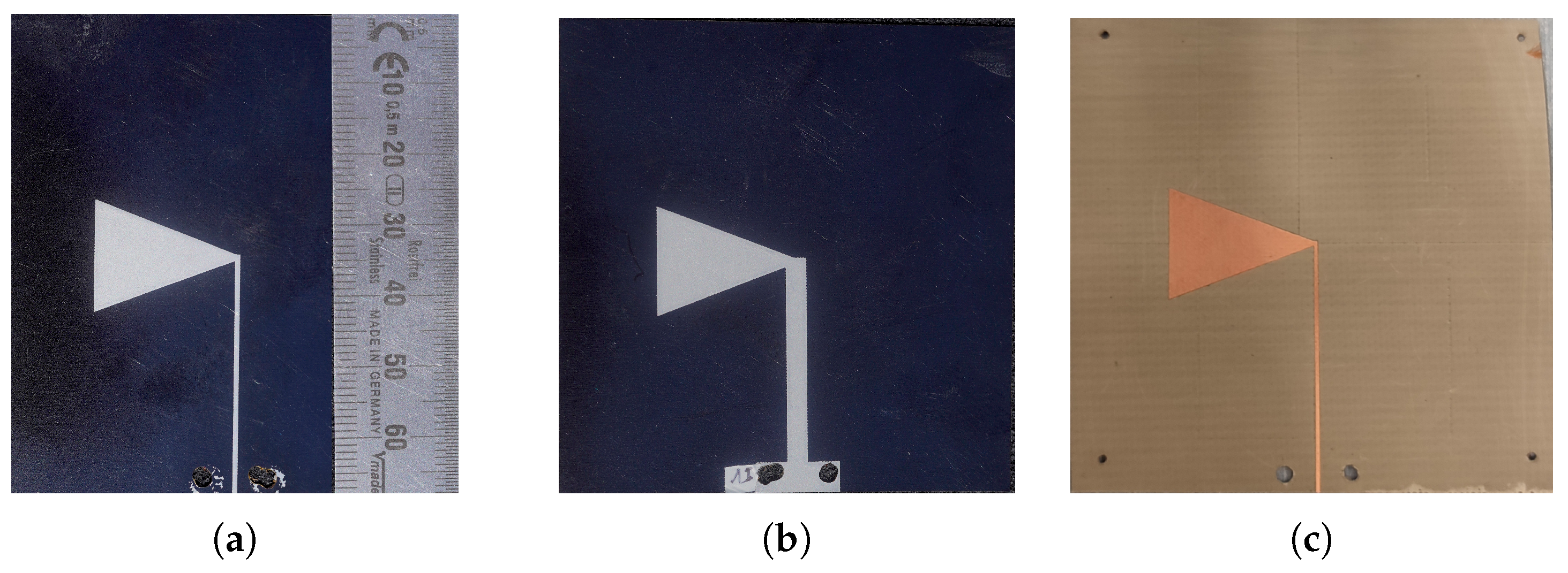
Figure 12 shows the photographs comparing the printed antenna with the copper-etched prototype. Figure 12a displays the top view, Figure 12b presents the bottom view, and Figure 12c shows the top view of the copper-etched version. These comparisons provide an overview of the fabrication process and the differences between the printed and laser-etched antennas.

Figure 12.
Photographs of the bow-tie antenna screen-printed on kapton: top layer (a), bottom layer (b) and laser etched (c).
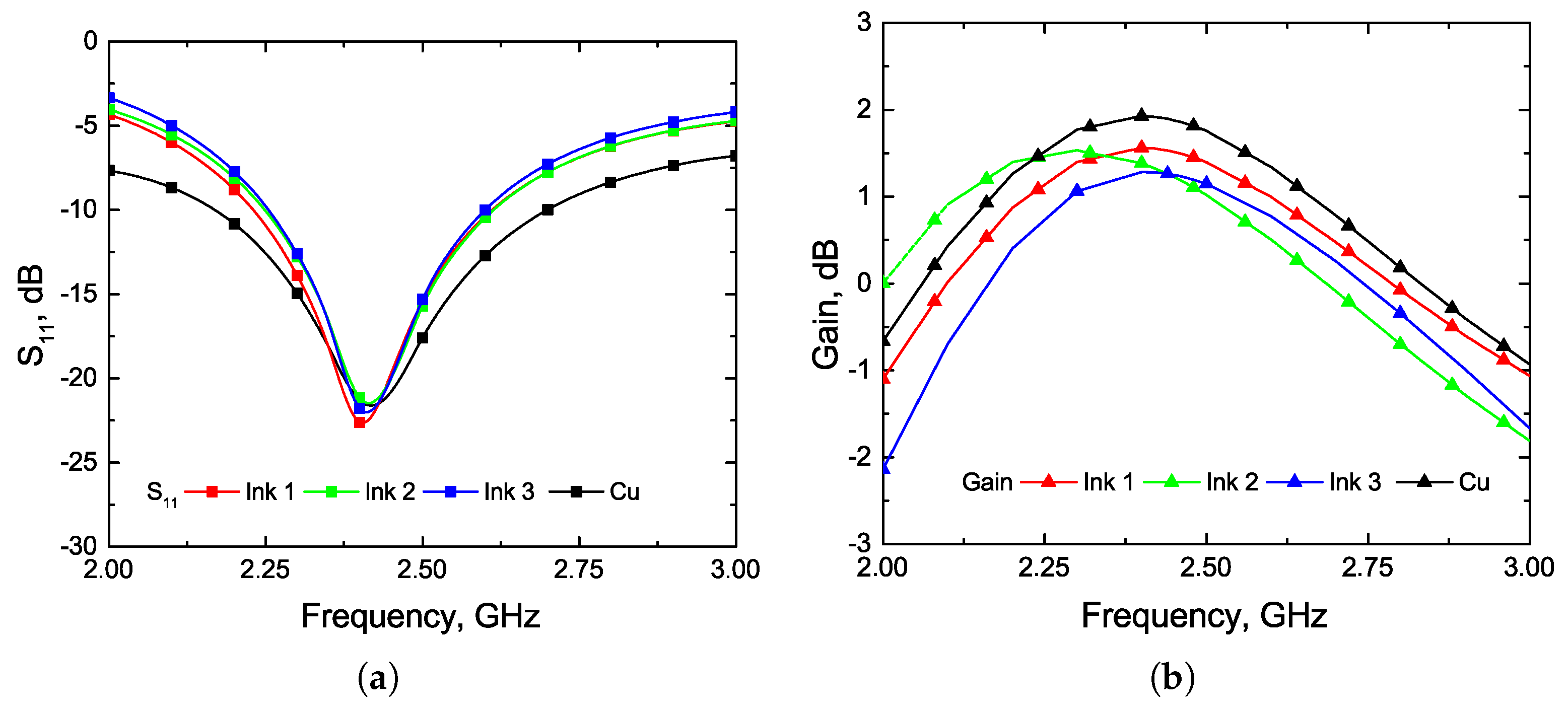
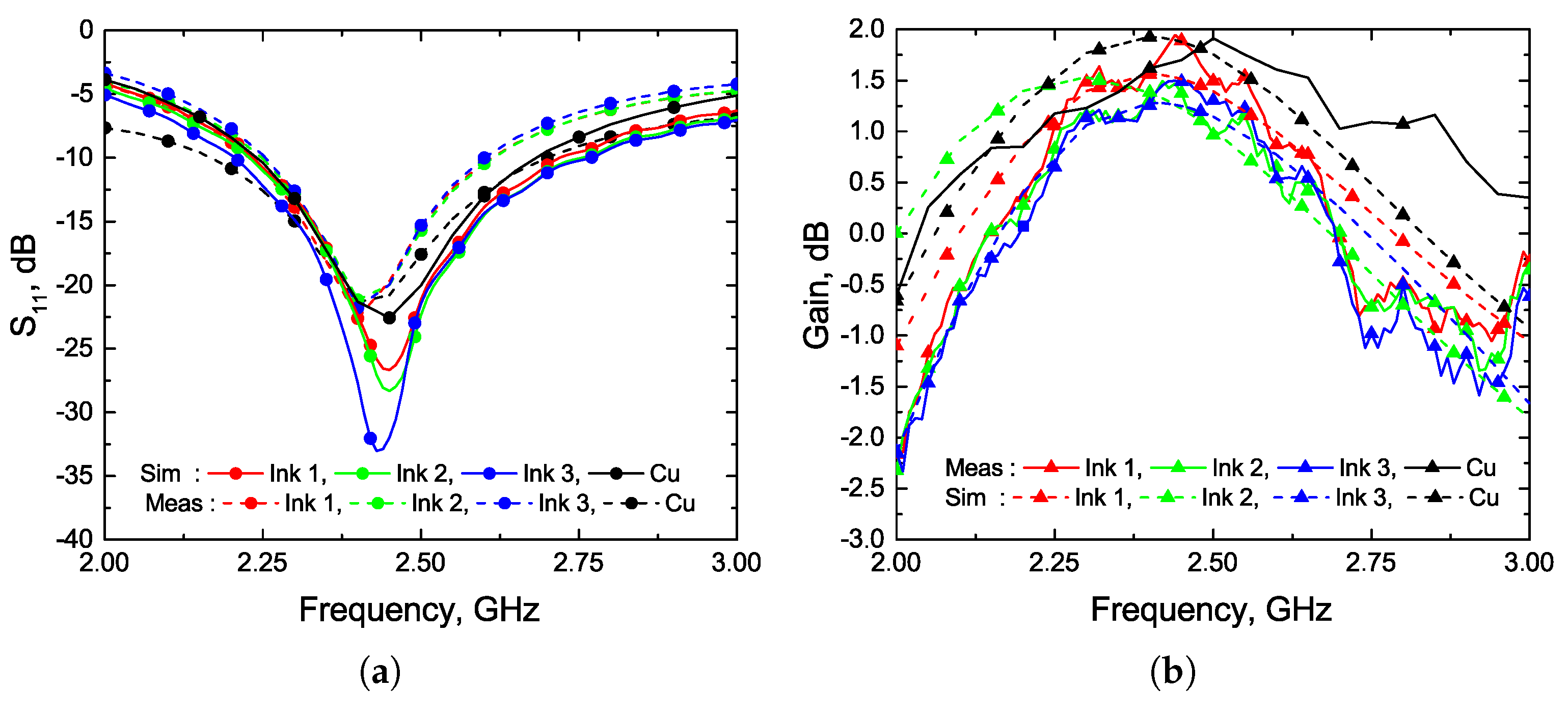
Simulations and measurements are depicted in Figure 13. As can be seen, slight frequencies shifts can be observed. The antennas are matched between for all considered inks and the etched copper prototypes.

Figure 13.
Measured and simulated (a) and gain (b) of the bow-tie antenna.
The measured gain ranges from 1.4 to for the prototypes, and it is for the copper-etched prototype. From the obtained results we may conclude that screen printing imperfections have no major impact on the antenna performances for the bow-tie antenna at . Additionally, the very low deviation of the measured and simulated gain between the screen-printed antennas and the etched copper version allows us to conclude that a careful selection of ink and its thickness does not significantly impact of the antenna performances.
4.2.2. The Bow-Tie Antenna
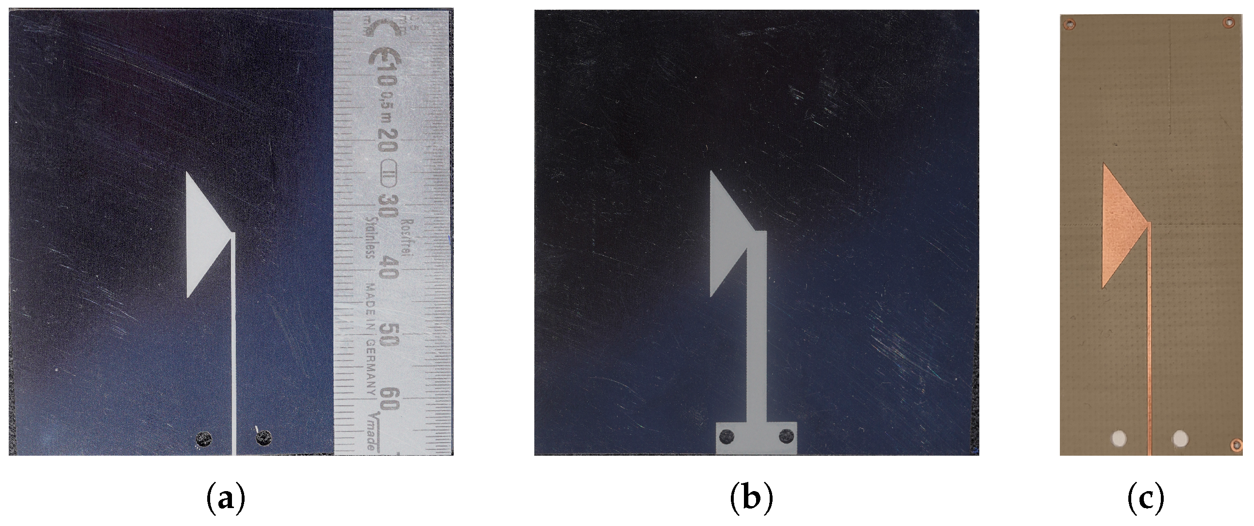
Figure 14 shows photographs comparing the printed antenna with the copper-etched prototype. Figure 14a displays the top view, Figure 14b presents the bottom view, and Figure 14c shows the top view of the copper-etched prototype. These comparisons offer an overview of the fabrication process and the differences between the printed and etched antennas.

Figure 14.
Photographs of the bow-tie antenna screen printed on kapton: top layer (a), bottom layer (b), and laser etched on taconic RF-35 (c).
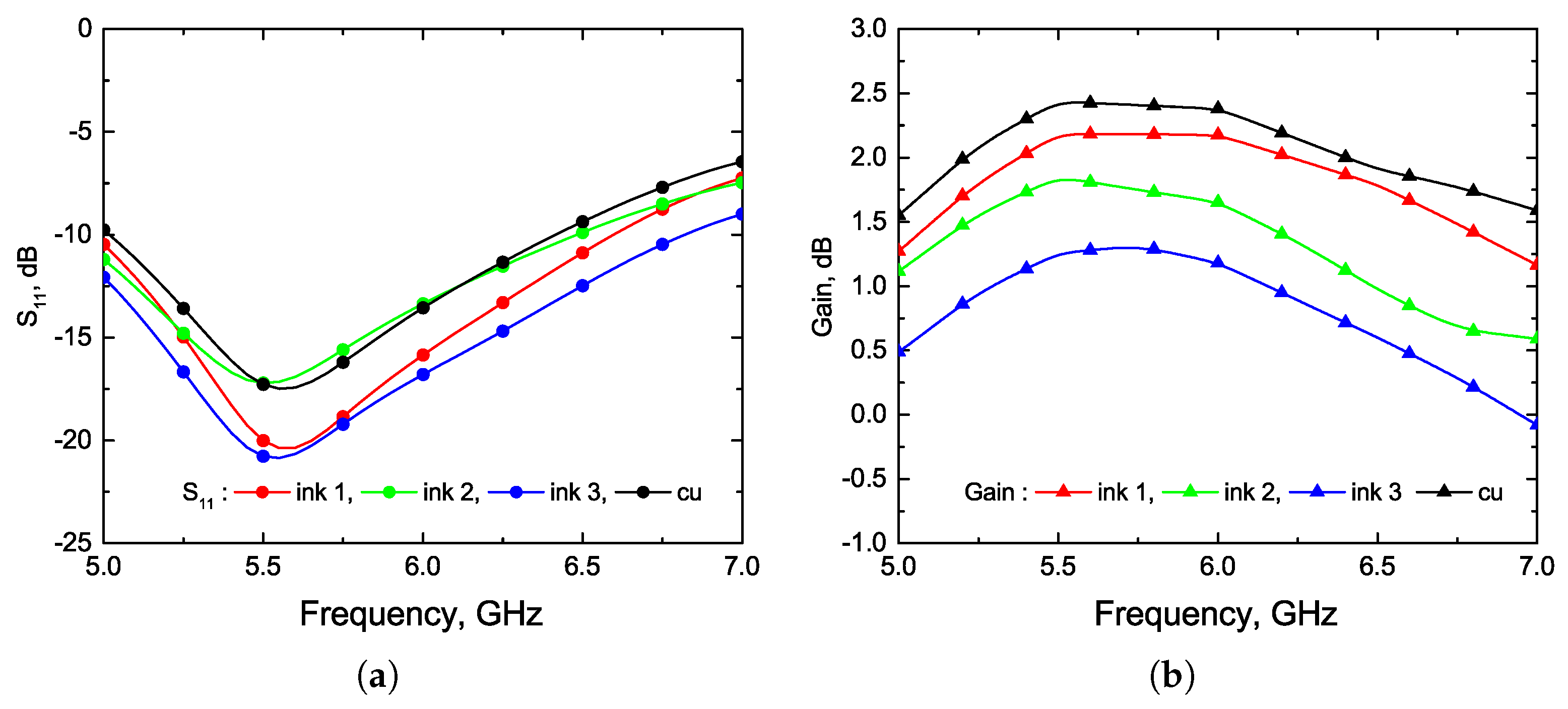
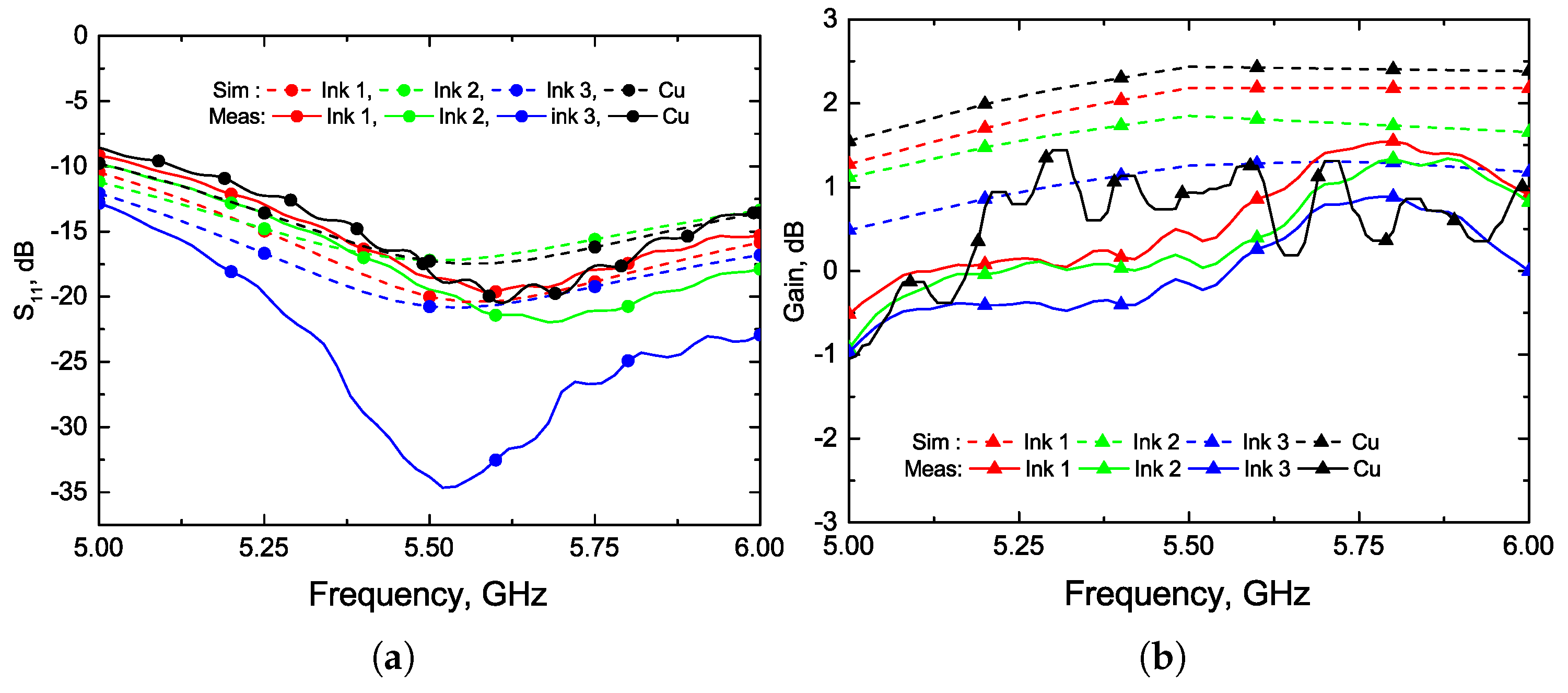
Measurements and simulations are plotted in Figure 15. The antenna matching bandwidth ranges from to for all considered inks and the copper-etched prototype. In Figure 15, the simulation and measurements are in very good agreement. The measured gain spans from to for the three prototypes and it achieved for the copper-etched configuration. As there is no significant frequency shift for the maximum gain or for matching bandwidth, these results confirm that geometrical screen-printing imperfections did not significantly impact the performances of bow-tie antenna.
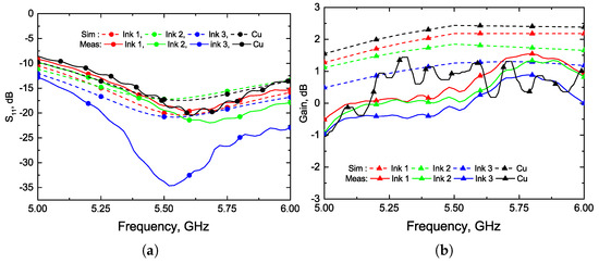
Figure 15.
Measured and simulated (a) and (b) gain of the bow-tie antenna.
Additionally, the very low deviation of the measured and simulated gain between the screen-printed antennas and the etched copper configuration allows us to conclude that a proper selection of ink and its thickness does not significantly influence the antenna performance. All measured performances are summarized in Table 6.
Table 6.
Summary of measured versus simulated performances of single band bow-tie antenna.
4.3. Circularly Polarized Bow-Tie Antenna
This section focuses on the comparison between measurements and simulation of circularly polarized antennas. These designs are characterized by dimensions closer to the resolution limit, particularly for the version. The smallest dimensions of the antenna structure pose a serious challenge since they come too close to the limits of the printing resolution.
4.3.1. CP Bow-Tie Antennas
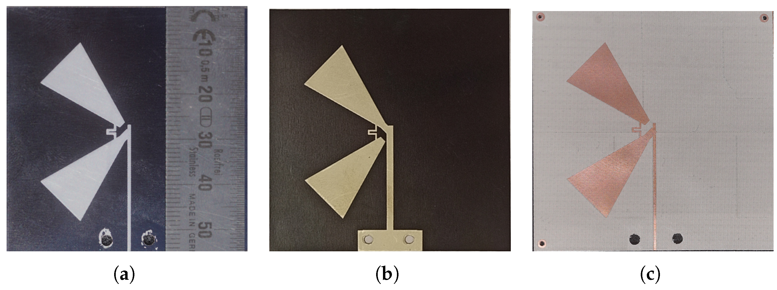
Figure 16 shows the photographs comparing the printed circularly polarized antenna with the copper-etched version. Figure 16a shows the top view, Figure 16b presents the bottom view, and Figure 16c depicts the top view of the copper-etched version.

Figure 16.
Photographs of the circularly polarized bow-tie antenna, screen printed on kapton: top layer (a), bottom layer (b), and laser etched on taconic RF-35 (c).
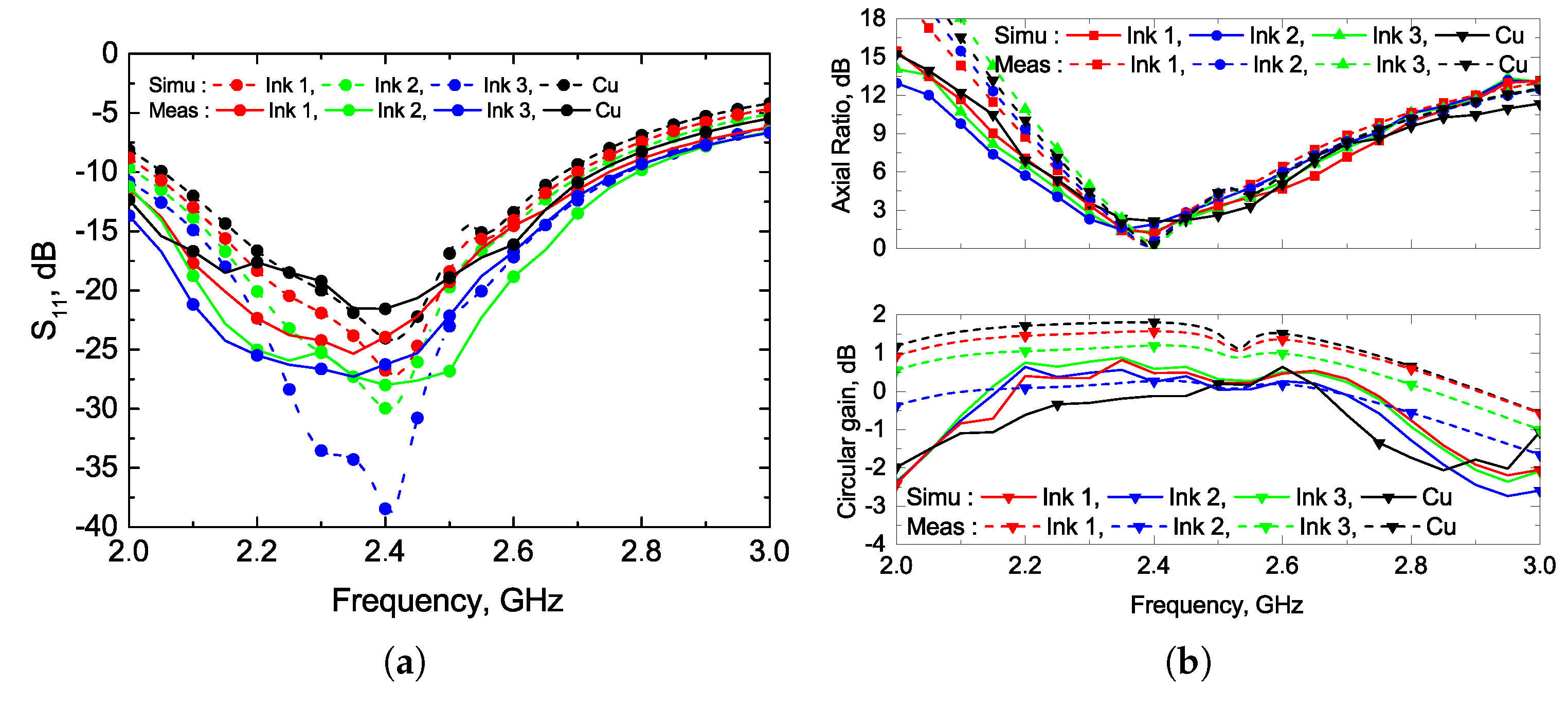
Antennas have been measured and all results are plotted on Figure 17a,b. As depicted in Figure 17a, the measured return loss is in accord with the simulations for all manufactured prototypes. All antennas are matched between and the measured gain values are very close for the three printed antennas, as shown in Figure 17a. The maximum measured circular gain varies from to . However, a slight difference in the axial ratio can be observed at frequencies beyond (see Figure 17b). All measured peak gain values are summarized in Table 7.

Figure 17.
Measured and simulated (a) and (b) axial ratio of the CP bow-tie antenna.
Table 7.
Summary of measured versus simulated performances of bi-band bow-tie antenna.
4.3.2. The CP Bow-Tie Antennas
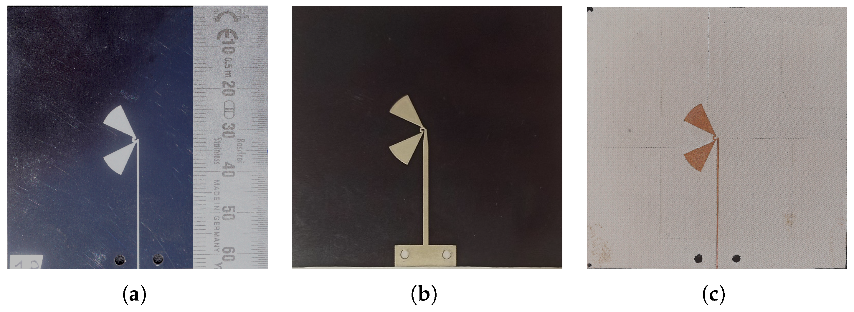
Figure 18 shows photographs comparing the printed circularly polarized antenna with the copper-etched prototype. Figure 18a shows the top view, Figure 18b presents the bottom view, and Figure 18c depicts the top view of the copper-etched configuration.

Figure 18.
Photographs of the CP bow-tie antenna: screen printed on kapton top layer (a), bottom layer (b), and laser etched on taconic RF-35 (c).
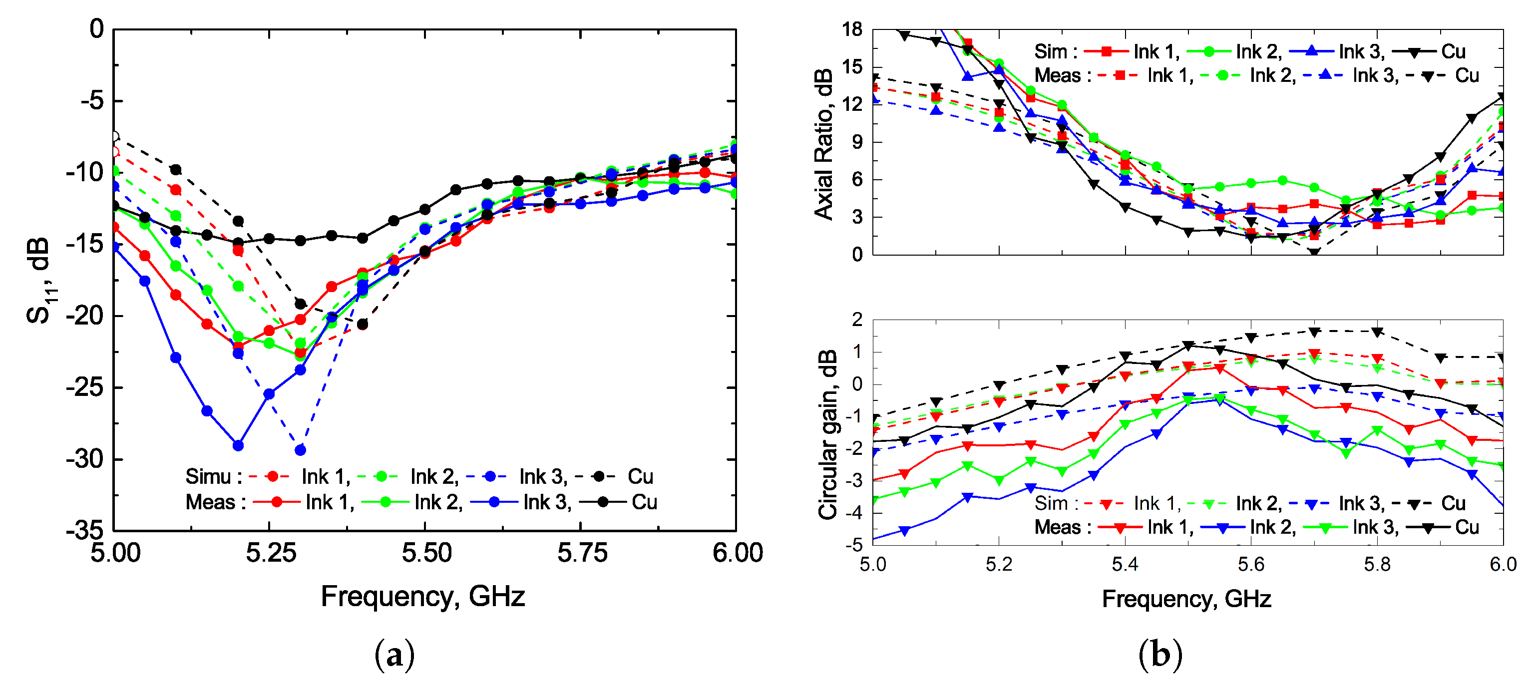
As shown in Figure 19a, the designed antenna is well-matched from 5 to , with slight differences between measurements and simulations. Those slight differences should be caused by the printing imperfections.

Figure 19.
Measured and simulated (a) , (b) circular gain and axial ratio of the CP bow-tie antenna.
Additionally, the measured gain is very close for the three printed antennas (see Figure 19a). The maximum measured circular gain ranges from to for the printed antennas and is for the copper-etched one. Nevertheless, discrepancies in axial ratio become notably more pronounced at compared to . In fact, a mismatch is observed within the frequency band where the axial ratio dips below in measurements (refer to Figure 19b). For this design some slight differences between measured figures of merit for the copper-etched and printed antenna begin to appear.
Upon careful examination of the antenna design, it becomes evident that the minimal length of the antenna is approaching the resolution limit of the screen printing process used to print the antennas. This closer proximity to the resolution limit may account for the discrepancies observed, particularly at higher frequencies. The observed divergence is significant enough to render the antenna circularly polarized outside the ISM band (see Figure 19b).
4.4. Bi-Band Bow-Tie Antenna
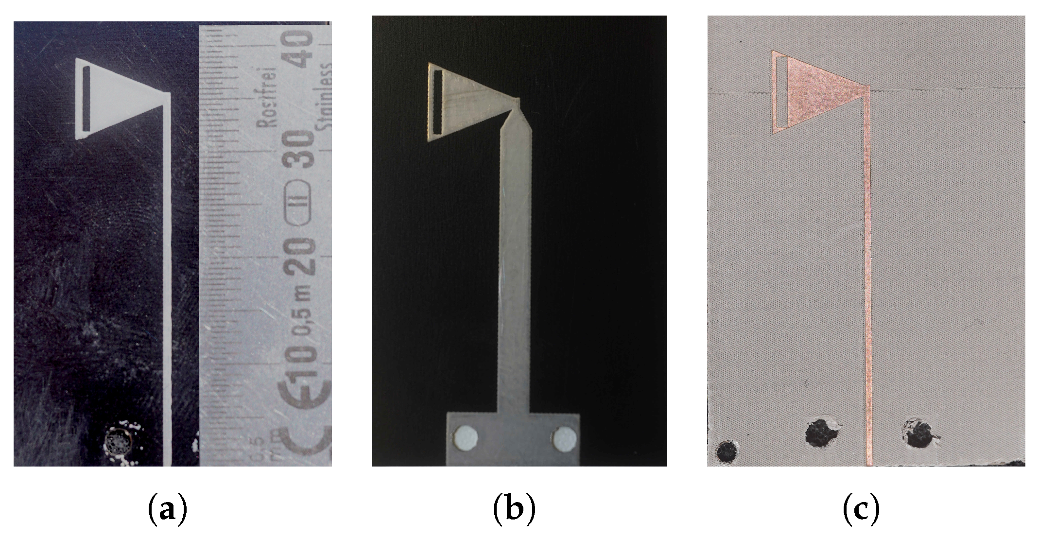
In this section, measurements are discussed and compared with simulation results of the bi-band bow-tie antenna. We focuses on that design, with dimensions close to the resolution limit. Photographs of the printed antenna are shown in Figure 20. A photo of the top layer is illustrated in Figure 20a, while Figure 20b shows a photo of the bottom layer. Additionally, Figure 20c depicts the Taconic-RF35 version of the antenna. These representations provide an overview of the fabrication process and highlight the differences between the printed and etched antennas.

Figure 20.
Photographs of the screen printed bi-band bow-tie antenna top (a) bottom (b), and top of the taconic RF-35 version (c).
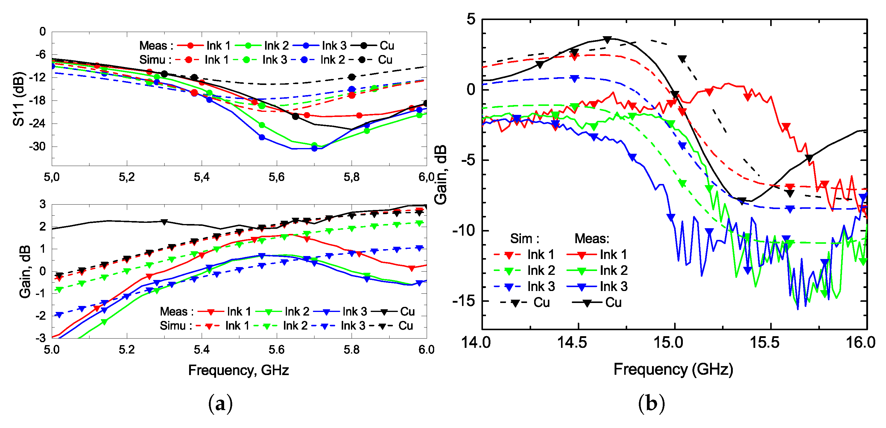
Measurements have been performed on the two frequency bands: from 5 to 6 GHz for the lowest band and from 14 to for the highest frequency band.
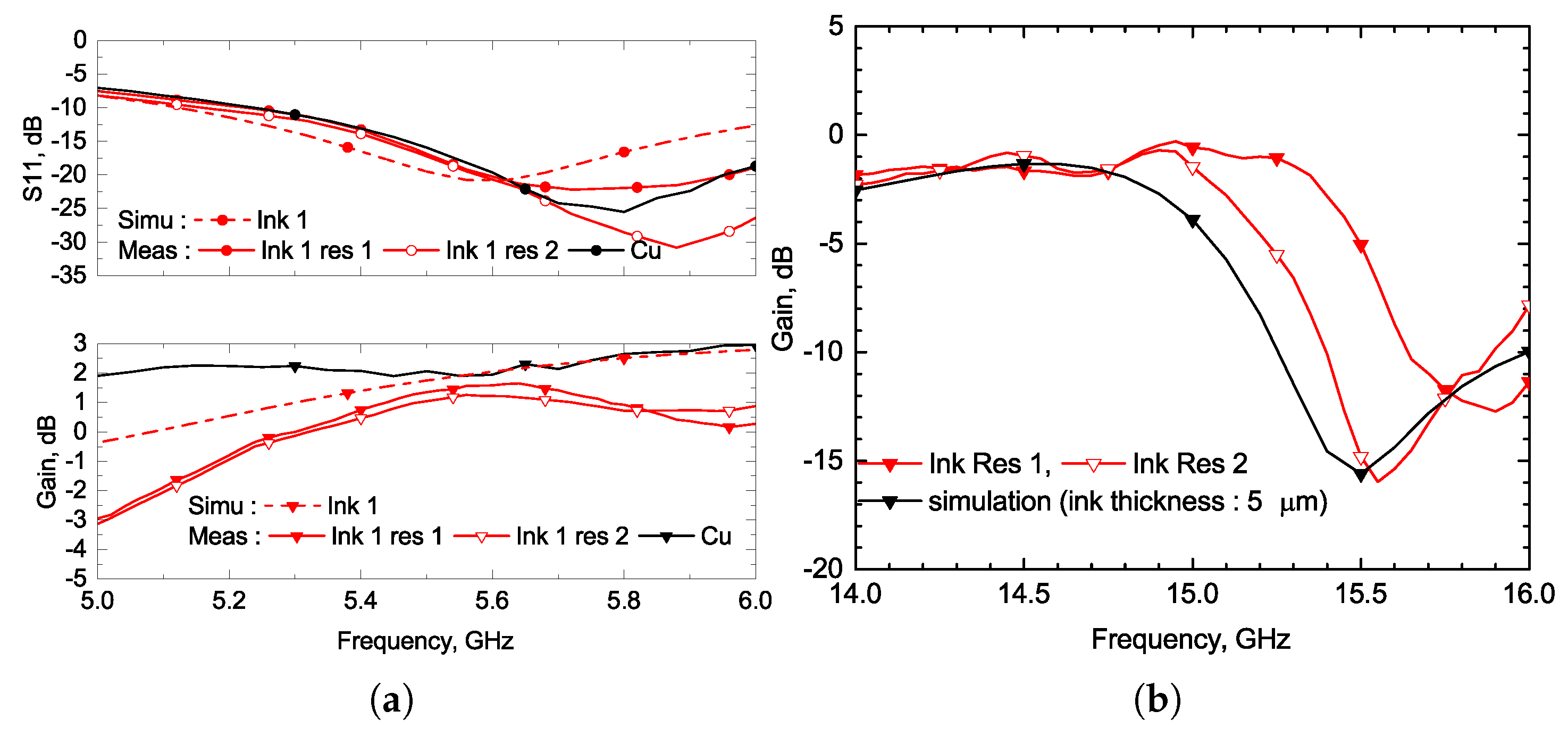
Measurements for the lowest frequency band are plotted in Figure 21a. Similarly to the linearly polarized antenna case, measurements agree well with the simulation results. All antennas are matched from to . The measurements in the higher band present a greater deviation from the simulations which is no longer acceptable in the context of antenna design. A frequency shift of about () and a reduction in peak gain are observed (see Figure 21b). All measured data are summarized in Table 8.

Figure 21.
Measured and simulated and gain (a) on the low frequency band and (b) on the high band of the bi-band bow-tie antenna.
Table 8.
Summary of measured versus simulated performances of bi-band bow-tie antenna.
4.5. Effect of Screen-Printing Resolution Improvement
A careful analysis of measurement results shows that a mismatch between simulations and measured data can be observed for the axial ratio of the CP bow-tie antenna. The axial ratio achieved is lower than 3 dB at higher frequencies than those predicted in simulations.
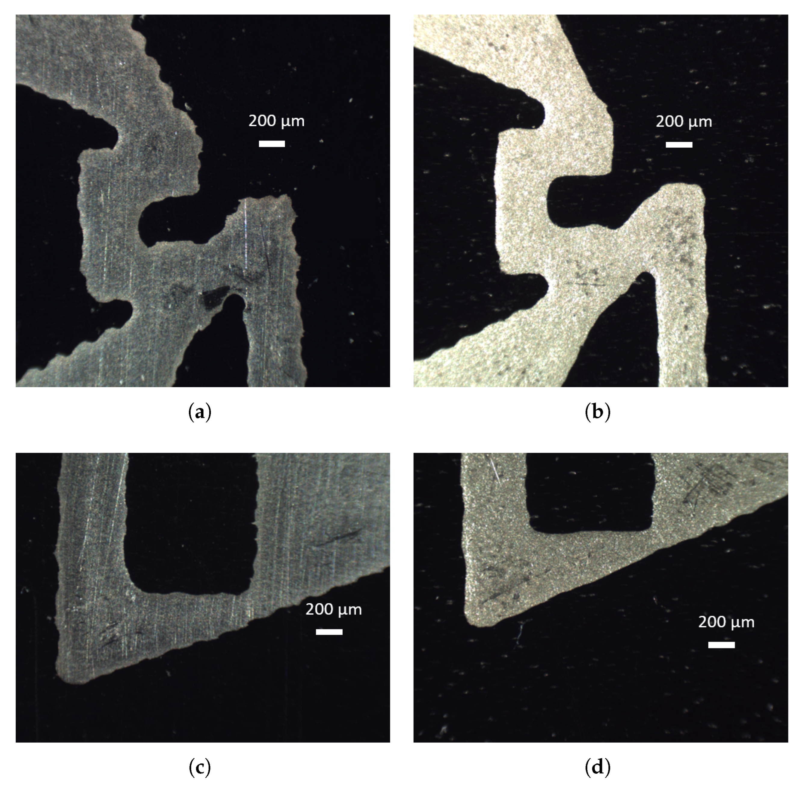
A careful examination of the printed CP bow-tie antenna reveals some printing issues on phase shifters, which are the smallest part of the antenna. Figure 22a gives detailed photographs of a phase shifter of the antenna. In this photograph we can see that the phase shifter is poorly printed: the corners are rounded and the lines do not have the proper width. In Figure 22b, the phase-sifter is better printed: the width of the line is correct the corners are less rounded. Similarly, for the bi-band bow-tie antenna, the frequency of peak gain is higher than expected for the highest operating frequency band. The same printing issues can be observed on the slot of the bi-band bow-tie antenna (see Figure 22c,d). In addition to the geometric analysis, complementary electromagnetic simulations were carried out. They aim to investigate the effect of varying for values between 3.2 and 3.8 (10%) on the axial ratio of the CP bow-tie antenna and on the gain of the dual-band antenna in the frequency band. The results plotted in Figure 23 show a less significant shift than those observed in the measurements. Moreover, the higher values of the axial ratio at and the gain drop observed in the measurement for the dual-band antenna do not appear in the simulation (see Figure 24a,b). Therefore, it is reasonable to conclude that a variation in the dielectric constant is not the main factor in the frequency shifts that occur at high-frequency measurements.

Figure 22.
Micro-photographs of a CP bow-tie phase-shifter (a) initial resolution, (b) improved resolution, and a slot of a bi-band bow-tie antenna (c) initial resolution, (d) improved resolution.
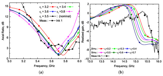
Figure 23.
Effect of modified resolution of printing on gain and of the CP bow-tie antenna (a) at (b) at .
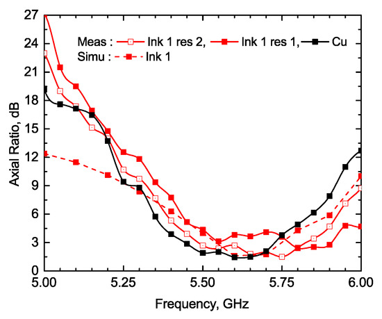
Figure 24.
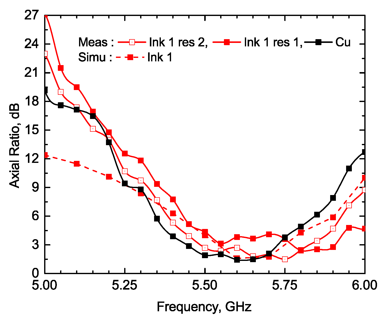
The effect of modified resolution of printing on AR of the CP antenna at .
To solve those mismatch problems an improvement of the screen printing resolution is investigated. In this way, the resolution is improved by decreasing the ink layer thickness to . Figure 24 shows the comparison between the measured AR of the two printing resolutions in the frequency band of to . An improvement in the results can be observed since the frequency shift is now only a few megahertz (less than (0.1%), whereas it was over (3 %) for the lower resolution. Furthermore, the measurement results of the gain in the same frequency band plotted in Figure 25a show that modifications of the printing parameters do not impact the measured gain. Note that the antenna has been re-simulated taking into account the reduction in the ink thickness.

Figure 25.
The effect of modified resolution of printing on gain and of the CP bow-tie antenna (a) at (b) at .
Given the previous results, we are now interested in the effects of reducing the thickness of the ink layers of the bi-band antennas in the high band. Figure 25b shows the measurement results of the gain in the to frequency band.
The measurement results of the gain in the to band plotted in Figure 25b. It shows that the frequency shift in the peak gain is greatly reduced from 3% to less than , but it is associated with a reduction of compared to the maximum gain value.
5. Conclusions
In this article, the impact of screen printing parameters on the performances of several bow-tie antennas (two single-band linearly polarized, two single-band CP, and a dual-band) has been investigated and measured. The influence of ink conductivity on peak gain has been studied using three different silver inks and compared with copper-engraved antennas. Antennas were printed using a cost-effective screen printing process developed at CEA-LITEN research center. However, the implemented antennas were characterized using the available facilities at IM2NP research center.
In light of the results obtained, we may conclude that with a proper selection of ink layer thickness, the peak gains obtained using the three inks are comparable to copper-engraved antennas up to . The second important result is that the limiting factor for operating at high frequency is the resolution of printed patterns. For low complexity antennas (linearly polarized and CP antennas), a good agreement between simulations and measurements has been observed. However, for higher complexity antennas such as bi-band antenna or CP bow-tie antenna, a disagreement of up to frequency shift of peak gain frequencies, has been observed. The resolution improvement of the printing process achieved with thinner ink layers can resolve these mismatch issues without influencing the measured peak gain at . All those results demonstrate the suitability of a cost-effective screen printing process for antenna manufacturing in the gigahertz frequency range.
Author Contributions
A.V. designed all antennas exept for the 5.8 GHZ CP bow-tie antenna. He performed all measurements under the supervision of M.E.; M.E. designed the 5.8 GHz CP bow-tie antenna. M.B. and C.S. suppervised all printing aspects. P.P.: review and supervision of Anton VENOUIL (AV). C.H.: review, editing, and co-supervision of Anton VENOUIL (AV). All authors participated in writing and reviewing the article. All authors have read and agreed to the published version of the manuscript.
Funding
This research received no external funding.
Institutional Review Board Statement
Not applicable.
Informed Consent Statement
Not applicable.
Data Availability Statement
Data are contained within the article.
Acknowledgments
This work is supported by the CEA Liten of Grenoble, France. The authors would likes to thanks David Alincant, for printing the prototypes presented in this article.
Conflicts of Interest
The authors declare no conflicts of interest.
References
- O’Sullivan, A.C.; Thierer, A.D. Projecting the Growth and Economic Impact of the Internet of Things. SSRN 2618794. 2015. Available online: https://www.mercatus.org/research/policy-briefs/projecting-growth-and-economic-impact-internet-things (accessed on 28 April 2025).
- Dahlavist, F.; Patel, M.; Rajko, A.; Shulman, J. Growing Opportunities in the Internet of Things; McKinsey & Company: New York, NY, USA, 2019; pp. 1–6. [Google Scholar]
- Khan, Y.; Thielens, A.; Muin, S.; Ting, J.; Baumbauer, C.; Arias, A.C. A new frontier of printed electronics: Flexible hybrid electronics. Adv. Mater. 2020, 32, 1905279. [Google Scholar] [CrossRef] [PubMed]
- Kim, J.; Kumar, R.; Bandodkar, A.J.; Wang, J. Advanced materials for printed wearable electrochemical devices: A review. Adv. Electron. Mater. 2017, 3, 1600260. [Google Scholar] [CrossRef]
- Abutarboush, H.F.; Li, W.; Shamim, A. Flexible-screen-printed antenna with enhanced bandwidth by employing defected ground structure. IEEE Antennas Wirel. Propag. Lett. 2020, 19, 1803–1807. [Google Scholar] [CrossRef]
- Nair, R.; Barahona, M.; Betancourt, D.; Schmidt, G.; Bellmann, M.; Höft, D.; Plettemeier, D.; Hübler, A.; Ellinger, F. A fully printed passive chipless RFID tag for low-cost mass production. In Proceedings of the The 8th European Conference on Antennas and Propagation (EuCAP 2014), The Hague, The Netherlands, 6–11 April 2014; IEEE: Piscataway, NJ, USA, 2014; pp. 2950–2954. [Google Scholar]
- Hasni, U.; Piper, M.E.; Lundquist, J.; Topsakal, E. Screen-printed fabric antennas for wearable applications. IEEE Open J. Antennas Propag. 2021, 2, 591–598. [Google Scholar] [CrossRef]
- Liang, J.; Guo, L.; Chiau, C.; Chen, X.; Parini, C. Study of cpw-fed circular disc monopole antenna for ultra wideband applications. IEE Proc.-Microw. Antennas Propag. 2005, 152, 520–526. [Google Scholar] [CrossRef]
- Salmerón, J.F.; Molina-Lopez, F.; Briand, D.; Ruan, J.J.; Rivadeneyra, A.; Carvajal, M.A.; Capitán-Vallvey, L.; de Rooij, N.F.; Palma, A.J. Properties and printability of inkjet and screen-printed silver patterns for RFID antennas. J. Electron. Mater. 2014, 43, 604–617. [Google Scholar] [CrossRef]
- Shin, D.-Y.; Lee, Y.; Kim, C.H. Performance characterization of screen printed radio frequency identification antennas with silver nanopaste. Thin Solid Film. 2009, 517, 6112–6118. [Google Scholar] [CrossRef]
- Blecha, T.; Linhart, R.; Reboun, J. Screen printed antennas on textile substrate. In Proceedings of the 5th Electronics System-Integration Technology Conference (ESTC), Helsinki, Finland, 16–18 September 2014; pp. 1–4. [Google Scholar]
- Ahmad, M.; Angeli, M.A.C.; Ibba, P.; Vasquez, S.; Shkodra, B.; Lugli, P.; Petti, L. Paper-based printed antenna: Investigation of process-induced and climatic-induced performance variability. Adv. Eng. Mater. 2023, 25, 2201703. [Google Scholar] [CrossRef]
- Arulmurugan, S.; Kumar, T.S.; Alex, Z.C. Screen printed high gain EBG-based wearable textile antenna for wireless medical band applications. Screen 2024, 123, 137–144. [Google Scholar] [CrossRef]
- Scarpello, M.L.; Kazani, I.; Hertleer, C.; Rogier, H.; Ginste, D.V. Stability and efficiency of screen-printed wearable and washable antennas. IEEE Antennas Wirel. Propag. Lett. 2012, 11, 838–841. [Google Scholar] [CrossRef]
- Ram, N.M.M.B.P.; Light, R.R.J. Design and testing of graphene-based screen printed antenna on flexible substrates for wireless energy harvesting applications. IETE J. Res. 2023, 69, 3604–3615. [Google Scholar] [CrossRef]
- Labiano, I.I.; Arslan, D.; Yenigun, E.O.; Asadi, A.; Cebeci, H.; Alomainy, A. Screen printing carbon nanotubes textiles antennas for smart wearables. Sensors 2021, 21, 4934. [Google Scholar] [CrossRef]
- Abdi, A.; Ghorbani, F.; Aliakbarian, H.; Geok, T.K.; Rahim, S.K.A.; Soh, P.J. Electrically small spiral pifa for deep implantable devices. IEEE Access 2020, 8, 158459–158474. [Google Scholar] [CrossRef]
- Xiao, B.; Wong, H.; Li, M.; Wang, B.; Yeung, K.L. Dipole antenna with both odd and even modes excited and tuned. IEEE Trans. Antennas Propag. 2021, 70, 1643–1652. [Google Scholar] [CrossRef]
- Jabber, A.A.; Jassim, A.K.; Thaher, R.H. Compact reconfigurable pifa antenna for wireless applications. TELKOMNIKA Telecommun. Comput. Electron. Control 2020, 18, 595–602. [Google Scholar] [CrossRef]
- Zalfani, N.; Beldi, S.; Lahouar, S.; Besbes, K. A miniaturized planar meander line antenna for uhf cubesat communication. Adv. Space Res. 2022, 69, 2240–2247. [Google Scholar] [CrossRef]
- de Mello, R.G.L.; Lepage, A.C.; Begaud, X. The bow-tie antenna: Performance limitations and improvements. IET Microw. Antennas Propag. 2022, 16, 283–294. [Google Scholar] [CrossRef]
- Nguyen, P.Q.; Yeo, L.-P.; Lok, B.-K.; Lam, Y.-C. Patterned surface with controllable wettability for inkjet printing of flexible printed electronics. ACS Appl. Mater. Interfaces 2014, 6, 4011–4016. [Google Scholar] [CrossRef]
- Denneulin, A.; Bras, J.; Blayo, A.; Neuman, C. Substrate pre-treatment of flexible material for printed electronics with carbon nanotube based ink. Appl. Surf. Sci. 2011, 257, 3645–3651. [Google Scholar] [CrossRef]
- Lukacs, P.; Pietrikova, A.; Vehec, I.; Provazek, P. Influence of various technologies on the quality of ultra-wideband antenna on a polymeric substrate. Polymers 2022, 14, 507. [Google Scholar] [CrossRef]
- Venouil, A.; Egels, M.; Benwadih, M.; Serbutoviez, C.; Pannier, P. Design guidance of a circularly polarized bowtie antenna for ISM bands. Microw. Opt. Technol. Lett. 2023, 65, 2972–2978. [Google Scholar] [CrossRef]
- Toh, B.Y.; Cahill, R.; Fusco, V.F. Understanding and measuring circular polarization. IEEE Trans. Educ. 2003, 46, 313–318. [Google Scholar]
- QRH20E Technical Specifications. 2024. Available online: https://www.rfspin.com/product/qrh20e/ (accessed on 28 April 2025).

Disclaimer/Publisher’s Note: The statements, opinions and data contained in all publications are solely those of the individual author(s) and contributor(s) and not of MDPI and/or the editor(s). MDPI and/or the editor(s) disclaim responsibility for any injury to people or property resulting from any ideas, methods, instructions or products referred to in the content. |
© 2025 by the authors. Licensee MDPI, Basel, Switzerland. This article is an open access article distributed under the terms and conditions of the Creative Commons Attribution (CC BY) license (https://creativecommons.org/licenses/by/4.0/).