Benchmarking Free Energy Calculations in Liquid Aliphatic Ketone Solvents Using the 3D-RISM-KH Molecular Solvation Theory

Abstract

The three-dimensional reference interaction site model of the molecular solvation theory with the Kovalenko–Hirata closure is used to calculate the free energy of solvation of organic solutes in liquid aliphatic ketones. The ketone solvent sites were modeled using a modified united-atom force field. The successful application of these solvation models in calculating ketone–water partition coefficients of a large number of solutes supports the validation and benchmarking reported here.

1. Introduction

The calculation of solvation free energy (SFE) is one of the cornerstones in chemistry, biology, and drug development efforts. The process of experimental solvation energy measurements is a tedious non-trivial process. Screening of solvation energy for a large number of compounds is time- and resource-consuming. Theoretical methods of calculation of SFEs have been developed over the years and are validated against experimental solvation free energy databases [1,2,3]. Such theoretical frameworks of solvation energy calculations encompass both explicit and implicit considerations of the environment provided by solvents [4,5,6]. A combination of these two models gave rise to the cluster-continuum model [7,8]. As with all theoretical models, these methodologies have limitations and drawbacks related to system size, type of molecules, and computational resource requirements. One of the statistical-mechanics-based molecular solvation theories, the three-dimensional reference interaction site model, a.k.a. 3D-RISM, has gained attention in the last couple of decades due to the proven applicability and accuracy of this theory in applications to (bio-)molecular simulations, material science applications, chemical reactivity problems, and inhomogeneous medium modeling [9,10,11,12,13,14,15,16,17,18,19,20].

The interaction site model has its origin in the works of Chandler and co-workers [21,22,23,24,25]. The detailed theoretical derivations and approximations of the theory of liquid state were reported elsewhere [26,27,28,29]. Here we will briefly explain the key points pertaining to the theoretical construct used for calculations. The RISM theory of molecular liquids is based on first principle statistical mechanics. The distribution of solvent sites around a solute of arbitrary shape and size is generated via the total correlation function h_γ(r), direct correlation function c_γ(r), and the site–site bulk susceptibility function χ_αγ(r) for α solvent sites around a solute at position r, as:

$$h_{\gamma }\left(\mathit{r}\right)={\displaystyle \sum }_{\alpha }{\displaystyle \int }d{\mathit{r}}^{\prime }{c}_{\alpha }\left(\mathit{r}-{\mathit{r}}^{\prime }\right){\chi }_{\alpha \gamma }\left(r^{\prime }\right)$$

(1)

The solute–solvent interaction potentials, u_γ(r), are related to the direct correlation function as: c_γ(r)~−u_γ(r)/(k_BT) with T and k_B are temperature and the Boltzmann constant, respectively. A simplified mathematical construct is needed to obtain the total and direct correlation functions to help integrate an infinite chain of inter- and intramolecular interactions and to impose a set of consistency conditions of the path-independent chemical potential μ. The bridge function(s) B_γ(r) used to achieve such transformations rewrites Equation (1) as:

h_γ(r) = exp(−u_γ(r))/k_BT + h_γ(r) − c_γ(r) + B_γ(r) − 1

(2)

A closure relation also helps simplifying mathematical and computational requirements in calculating the bridging function. In this work, we have used the well-established Kovalenko–Hirata (KH) closure relations for all RISM calculations [30]. The functional form of the KH closure is given as:

$$g_{\gamma }\left(\mathit{r}\right)=\{\begin{array}{ccc}exp\left(-u_{\gamma }\left(\mathit{r}\right)/\left(k_{\mathrm{B}}T\right)+h_{\gamma }\left(\mathit{r}\right)-c_{\gamma }\left(\mathit{r}\right)\right)& \mathrm{for}& g_{\gamma }\left(\mathit{r}\right)\le 1\\ 1-u_{\gamma }\left(\mathit{r}\right)/\left(k_{\mathrm{B}}T\right)+h_{\gamma }\left(\mathit{r}\right)-c_{\gamma }\left(\mathit{r}\right)& \mathrm{for}& g_{\gamma }\left(\mathit{r}\right)>1\end{array}$$

(3)

The excess chemical potential (and hence the solvation energy) is obtained using closed analytical expression as:

$${\mu }_{\mathrm{solv}}={{\displaystyle \sum }}_{\gamma } {\int }_{V}d\mathit{r} {\Phi }_{\gamma }\left(\mathit{r}\right) \mathrm{and} {\Phi }_{\gamma }\left(\mathit{r}\right)={\rho }_{\gamma }{k}_{B}T\left[\frac{1}{2}{h}_{\gamma }^2\left(\mathit{r}\right)\mathsf{\Theta }\left(-h_{\gamma }\left(\mathit{r}\right)\right)-c_{\gamma }\left(\mathit{r}\right)-\frac{1}{2}{h}_{\gamma }\left(\mathit{r}\right)c_{\gamma }\left(\mathit{r}\right)\right]$$

where Θ is the Heaviside step function.

The other important physical properties, partial molar volume (PMV, Ṽ) and isothermal compressibility (χ_T), are computed using the number density (ρ) as:

$$Ṽ=k_{\mathrm{B}}T{\chi }_T(1-{{\displaystyle \sum }}_{\gamma }{\rho }_{\gamma }\int d\mathit{r}{c}_{\gamma }\left(\mathit{r}\right)) \mathrm{and} {\rho }_{\mathrm{total}}{k}_{\mathrm{B}}T{\chi }_T={(1-4\pi {{\displaystyle \sum }}_{\alpha \gamma }{\rho }_{\alpha }{\int }_0^{\infty }{r}^{2}dr c_{\alpha \gamma }\left(r\right) )}^{-1}$$

The 3D-RISM-KH theory can produce solvation structures efficiently, although the internal pressure computed is wrong since the formulation of RISM theory. Further, the maxima on the partial distribution functions were shifted and broadened, as shown in other reports using this theory. One way to correct the Gaussian fluctuation solvation free energy (ΔG_GF) to get correct correlation to experimental data is to use a “universal correction” scheme using the 3D-RISM computed PMVs as [31]:

ΔG_corrected = ΔG_GF + a × PMV + b

The coefficients a and b are obtained from linear regression analysis against known solvation energies. The success of this correction scheme depends on the availability of a sufficient number of solvation free energy values in benchmark dataset(s).

The 3D-RISM-KH theory was successfully applied to calculate SFEs in a broad range of solvents previously, with both low- and high-polarity solvents. In this report, we have selected four aliphatic liquid ketones to standardize application in free energy calculation with the 3D-RISM-KH theory. Ketones are an important class of compounds with applications as solvents, polymer building blocks, pharmaceutical ingredients, etc. We have chosen four different aliphatic ketones, viz. acetone, butanone (methyl ethyl ketone), methyl isobutyl ketone (4-Methyl-2-pentanone), and cyclohexanone in this study due to the availability of a sufficient number of experimental solvation energy data to calibrate 3D-RISM-KH calculations and to further validate the results against experimental ketone-water partition coefficient calculations.

2. Materials and Methods

Electronic structure calculations: All of the solute molecules used for the solvation energy calculations were optimized at the M06-2X/Def2-TZVPP level in the gas phase as well as in cyclohexanone (CyO), butanone (MEK), and methyl isobutyl ketone (MIBK) continuums [32,33]. The solvent effects were incorporated using the conductor-like polarizable continuum model (CPCM) and the SMD solvation models [34,35,36]. All the quantum mechanics (QM) calculations were performed using the Gaussian16 software package with default settings [37]. All the optimized structures were verified as minima on the respective potential energy surface via vibrational mode analysis.

Molecular dynamics (MD) simulations: All the MD simulations were performed using the GROMACS simulation package [38]. The all-atom GAFF force fields with the AM1-BCC charges were used to model the liquid states of the ketone [39,40]. A solvent box containing 256 ketone molecules was created and equilibrated for a total of 2 ns at a temperature of 298 K and a pressure of 1 bar using a Berendsen thermostat without any geometrical constraints for stable temperature and density profiles. The final production runs were of 10 ns for each system. All of the distribution functions were calculated using the standard utilities incorporated in the GROMACS package.

RISM calculations: A united-atom model of the liquid ketones was used for all the RISM calculations using previously reported parameters [41,42]. Atomic charges obtained from quantum chemical calculations at the MP2/cc-pVTZ level were used to assign partial charges to solvent sites [43,44]. The solvent susceptibility functions of the liquid ketones were computed using the extended-RISM (XRISM) formalism at 298 K. A tolerance criterion of 1 was used for the convergence of solvent distribution function calculations. The cyclohexanone system failed to converge with the united atom parameters. Such behavior was reported earlier by Luchko et al. for a cyclohexane system [45]. Those authors have developed united-atom parameters for C[H₂]-centers in cyclohexane. In this work we have adopted those parameters for cyclohexanone C[H₂] centers. For water, the DRISM theory is used with the modified SPCe water model. Please refer to

Table 1. Van der Waal’s parameters used for solvent atomic sites in this study.

Atomic Site	σ (Å)	ε (kcal·mol−1)
C[H3]	3.775	0.207
C[H2]	3.905	0.118
C[H]	3.850	0.080
C[=O]	3.399	0.086
O[=C]	2.960	0.210
OWater	3.116	0.155
HWater	0.700	0.046
C[H2]Cyclohexanone	4.700	0.140

for the force field parameters used for the solvent molecules reported in this study. The lowest energy conformation of the solutes for the molecular partition coefficient calculations were generated using the MMFF94 force field [46,47], and were used for all the 3D-RISM-KH calculations. All of the solutes were parameterized using the GAFF force field with the AM1-BCC charges. The 3D-RISM-KH calculations on the solutes were performed on a uniform cubic 3D-grid of 128 × 128 × 128 points in a box of size 64 × 64 × 64 ų representing a solute with a few solvation layers with convergence accuracy set to 10⁻⁵ of the modified direct inversion in the iterative subspace (MDIIS) solver. All the RISM calculations were conducted with our in-house code, a working version of which is available in the AMBERTOOLS utility. The partition coefficients between acetate esters and water were calculated as:

$$\log P_{\mathrm{ester}-\mathrm{water}}=-\frac{\Delta G_{\mathrm{ester}}-\Delta G_{\mathrm{water}}}{k_{\mathrm{B}} T ln10}$$

Solute Databases: For solvation free energy calculations in butanone, methyl isobutyl ketone, and cyclohexanone, the experimental data were taken from the Minnesota Solvation Database [48]. The ketone–water partition coefficient data for acetone, butanone, methyl isobutyl ketone, and cyclohexanone to water partitioning were taken from the work of Abraham et al. [49]. The experimental hydration free energies were taken from the FreeSolv database [50].

3. Results

In this manuscript, we have benchmarked the performance of the 3D-RISM-KH molecular solvation theory in predicting the solvation free energy of organic solutes in liquid aliphatic ketones, butanone (MEK), methyl isobutyl ketone (MIBK), and cyclohexanone (CyO) using the united-atom amber force field parameters. A correction scheme is developed to predict solvation free energy in liquid ketones. This correction scheme is used to calculate ketone–water partition coefficients for a large set of organic molecules. Our findings are divided as follows: the first section provides a comparative picture of the liquid structures of four ketones obtained from the all-atom MD simulations and the XRISM-KH calculations; the following sections detail the SFE calculations using the QM calculations and the 3D-RISM-KH calculations, and a comparison between different computation schemes; the third and final section provides a proof of concept of a successful application of the 3D-RISM-KH theory in predicting ketone–water partition coefficients.

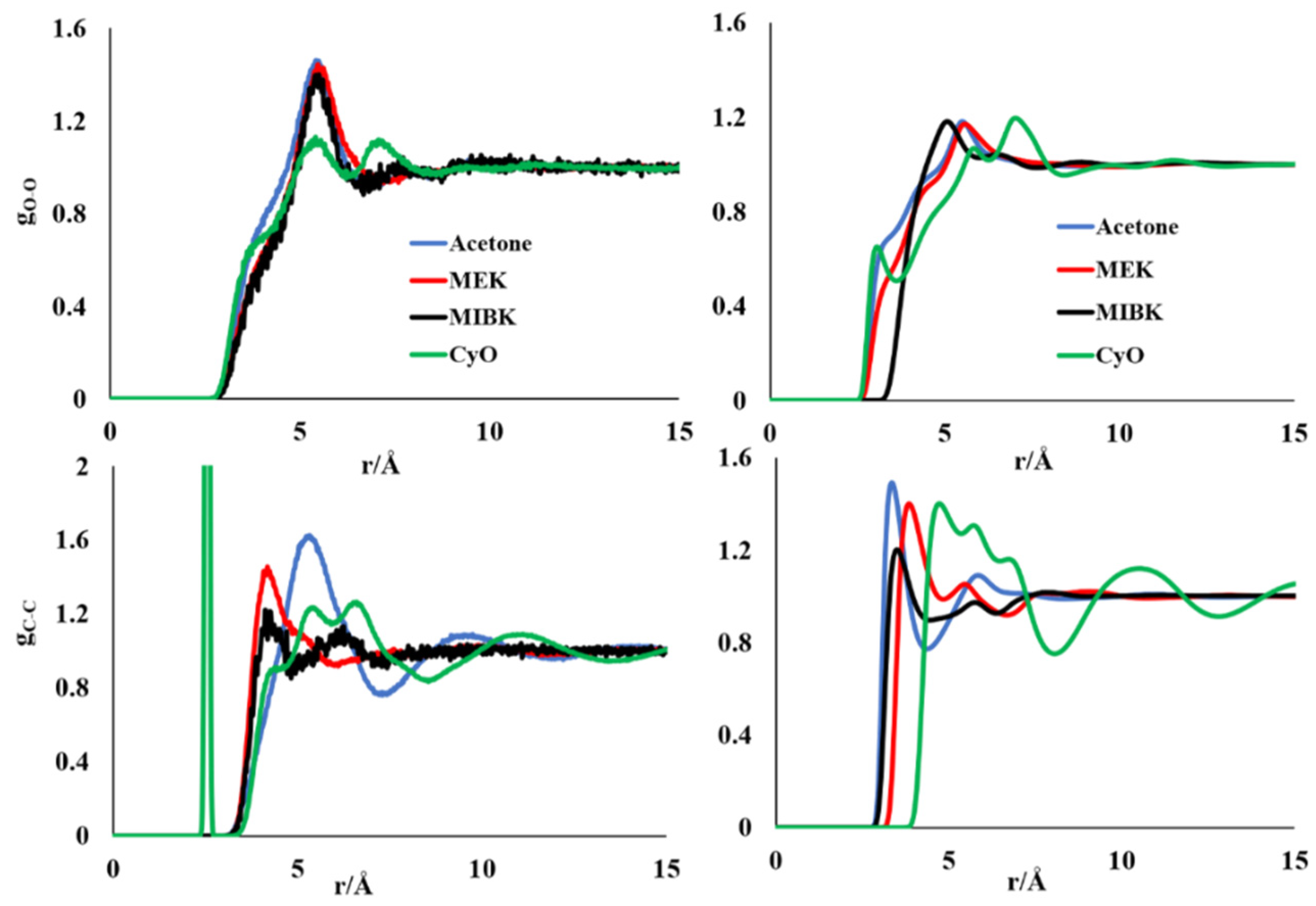
3.1. Molecular Simulations of Pure Liquid Ketones

The liquid state of four ketones, acetone, MEK, MIBK, and CyO, are simulated with all-atom MD. The MD equilibration runs provided satisfactory results for density profiles for all of the ketones in the temperature range of 298 K. The findings are summarized in

Table 2. Experimental and MD computed physical characteristics of the liquid ketones.

Molecule	Density (Experimental, gm/cm3)	Density (MD, gm/cm3) 1	Dielectric Constant (Experimental)
Acetone	0.784	0.782 (±0.0009)	20.493
MEK	0.805	0.784 (±0.0006)	18.246
MIBK	0.796	0.800 (±0.0003)	12.887
CyO	0.942	0.929 (±0.0008)	15.619

¹ Error estimates from MD simulations are provided in parentheses.

. It is important to note that the dielectric constant and density of the liquid state are inputs for XRISM-KH calculations. The first check of the quality of solvent susceptibility function calculations using the XRISM-KH theory is performed by confirming that all the isothermal compressibilities of liquid ketones under study are positive at 298 K. A negative isothermal compressibility would otherwise be indicative of a non-physical nature of the solution(s) obtained at this level of theory.

The liquid structures of four ketones as shown from the radial distribution functions present distinctive features between cyclic- and non-cyclic ketones (Figure 1). For example, the first maxima in the carbonyl oxygen distribution are around 5.4 Å for acetone, MEK, and MIBK, with a pre-peak shoulder in the 4–5 Å region. The same radial distribution for CyO have two equal-density broad peaks at 5.4 Å and 7.2 Å. The second peak for the three acyclic ketones are of much less intensity than the first maxima. The features in the carbonyl oxygen partial distribution functions obtained using the XRISM-KH theory showed similar features as those obtained with the all-atom MD simulations, although with some differences. First, the CyO distribution has a first maximum around 3.1 Å, followed by two other peaks around 5.9 Å and 7.1 Å. The peak around 5.1 Å has the smallest intensity. The carbonyl carbon center (C[=O]) of ketones showed unique features based on the identity of the molecule, as described below. The MD computed maxima for acetone are around 5.4 Å and 9.5 Å. In the XRISM-KH calculations, the maxima are around 3.4 and 6 Å. For the MEK system, the first maxima in the MD RDF is around 4.2 Å, s with a broad hump in the 7–9 Å region. The RISM profile of the carbonyl carbon of MEK had maxima at 3.9 Å and 5.6 Å, and the broad hump was located in the 7–9 Å. The MD-computed rdfs for the MIBK carbonyl carbon has maxima around 4.6 and 6.1 Å. The same distributions from the XRISM calculations are located about 3.6 and 6.1 Å. The profile of the carbonyl carbon of CyO showed stark differences from that of other ketones. The MD simulations picked the first maxima around 2.5 Å, with multiple minima between 4.4 and 8.6 Å and a broad peak in the region of 10–13 Å. The XRISM distribution showed multiple peaks in the CyO carboyl carbon distribution in the region of 4.7–7 Å, with a broad peak in the 10–13 Å region. Overall, the MD- and XRISM-KH-computed distributions of solvent sites for individual ketones are qualitatively similar. The differences in the computed distribution profiles between these two computational methods can be atrributed to the choice of the force field (all-atom in MD vs. united atom in XRISM-KH) and other theoretical artifacts associated with molecular simulation methods. The difference in the distribution profile between the three acyclic ketones (viz. acetone, MEK, and MIBK) and the cylohexanone are indicative of different liquid structures for these two (sub)classes of compounds. Hence, we have decided to scale the solvation behavior differently for the cyclic- and acyclic-ketones in this study.

3.2. Solvation Free Energy Calculations

The solvent susceptibility functions computed using the XRISM-KH theory for MEK, MIBK, and CyO are used to calculate the SFEs of small organic molecules in these three solvents using the 3D-RISM-KH theory. There is a total of thirty-six experimental SFE values available in the Minnesota Solvation Database, out of which 10 are SFEs in CyO, and 13 experimental SFEs, each for MEK and MIBK. As mentioned in the previous section, due to the differences in the liquid structures between cyclic and acyclic ketones, we have used the “universal correction” scheme for the combined SFE datasets for MEK and MIBK, while the SFEs of CyO were calibrated separately. The coefficients for the “universal correction” scheme of SFEs are provided in

Table 3. Regression coefficients for correcting the GF-solvation free energy.

Molecule	A (kcal·mol−1·Å−3)	B (kcal·mol−1)
Acyclic aliphatic ketone	0.0016	−4.2669
Cyclohexanone	−0.2286	−5.0964

. It is important to note that the fitting coefficients are dependent on the accuracy of the benchmark dataset, as well as the number of data points used in the regression analysis.

The solute dataset reported here was used for the development of the SMD solvation model, and hence, the best results in the SFE calculation were obtained using the QM calculations in the SMD model with an overall relative mean square error (RMSE) of 1.33 kcal/mol. The other atomic surface-charge-based QM solvation model, i.e., CPCM, yielded a RMSE of 2.71 kcal/mol. The 3D-RISM-KH-computed corrected SFE has an overall RMSE of 1.51 kcal/mol. The performance of the 3D-RISM-KH theory in calculating SFEs is on par with that of the state-of-the-art QM SFE calculation methods. The 3D-RISM-KH method requires less computational resource requirements than QM calculations. The experimental and computed SFEs are provided in

Table 4. Experimental and computed SFEs (in Kcal/mol) in various liquid ketones.

Compound	Solvent	ΔG(Exptl.) 1	ΔG(CPCM) 2	ΔG(SMD) 3	ΔG(RISM) 4
n-octane	Cyclohexanone	−4.57	−0.64	−4.13	−3.37
Toluene	Cyclohexanone	−5.05	−2.88	−6.43	−4.45
Ethanol	Cyclohexanone	−4.41	−3.09	−3.83	−5.02
1,4-dioxane	Cyclohexanone	−4.95	−3.37	−5.30	−7.02
2-butanone	Cyclohexanone	−4.42	−2.35	−5.27	−5.32
Acetic acid	Cyclohexanone	−6.43	−4.60	−6.03	−6.32
Propanoic acid	Cyclohexanone	−7.18	−4.30	−6.42	−6.24
Nitromethane	Cyclohexanone	−5.09	−5.42	−5.77	−6.70
Cyclohexanone	Cyclohexanone	−6.25	−4.12	−7.99	−6.64
Hydrogen peroxide	Cyclohexanone	−9.11	−4.60	−7.62	−6.39
n-octane	Butanone	−4.64	−0.64	−5.21	−2.26
Toluene	Butanone	−5.06	−2.90	−7.26	−3.71
Ethanol	Butanone	−4.46	−3.13	−4.34	−4.46
1,4-dioxane	Butanone	−5.02	−3.41	−5.96	−6.29
Formaldehyde	Butanone	−1.77	−3.17	−3.22	−4.82
2-butanone	Butanone	−4.5	−2.40	−5.96	−4.71
Acetic acid	Butanone	−6.88	−4.65	−6.51	−5.99
Propanoic acid	Butanone	−7.05	−4.35	−7.00	−5.88
Butanoic acid	Butanone	−7.34	−4.40	−7.63	−5.83
Pentanoic acid	Butanone	−7.54	−4.55	−8.37	−5.80
Hexanoic acid	Butanone	−8.07	−4.61	−9.09	−5.76
Nitromethane	Butanone	−5.24	−5.49	−6.37	−6.15
γ-butyrolactone	Butanone	−4.47	−6.50	−9.69	−8.12
Naphthalene	Methyl isobutyl ketone	−7.45	−2.55	−8.29	−7.26
Phenol	Methyl isobutyl ketone	−9.38	−3.98	−7.86	−7.13
m-Cresol	Methyl isobutyl ketone	−8.79	−4.24	−8.15	−7.27
Acetic acid	Methyl isobutyl ketone	−6.33	−4.53	−6.35	−6.49
Propanoic acid	Methyl isobutyl ketone	−6.85	−4.23	−6.89	−6.68
Butanoic acid	Methyl isobutyl ketone	−7.44	−4.28	−7.55	−6.98
Trimethylamine	Methyl isobutyl ketone	−2.86	−1.46	−3.44	−5.08
Diethylamine	Methyl isobutyl ketone	−3.63	−1.99	−4.86	−5.01
Pyridine	Methyl isobutyl ketone	−5.33	−3.11	−6.36	−6.37
Aniline	Methyl isobutyl ketone	−7.54	−4.03	−8.50	−7.25
Ammonia	Methyl isobutyl ketone	−2.52	−3.15	−3.57	−3.80
Methylamine	Methyl isobutyl ketone	−4.14	−2.55	−3.45	−4.25
4-methyl-2-pentanone	Methyl isobutyl ketone	−5.23	−3.74	−7.39	−6.18
MAD 5			2.41	0.98	1.21
RMSE 6			2.71	1.33	1.51

¹ Experimental solvation free energy. ² SFEs computed at the CPCM/M06-2X/Def2-TZVPP level. ³ SFEs computed at the SMD/M06-2X/Def2-TZVPP level. ⁴ SFEs computed using the 3D-RISM-KH theory with solute geometries from the Minnesota Solvation Database. ⁵ Mean absolute deviation: $\mathrm{MAD}=\frac{1}{\mathrm{n}}{\sum }_1^{\mathrm{n}}\left|{\mathrm{x}}_{\mathrm{i}}-\mathrm{x}\right|$. ⁶ Relative mean square error: $RMSE=\sqrt{\frac{1}{n}}{\sum }_1^n{\left(x_i-x\right)}^2$.

.

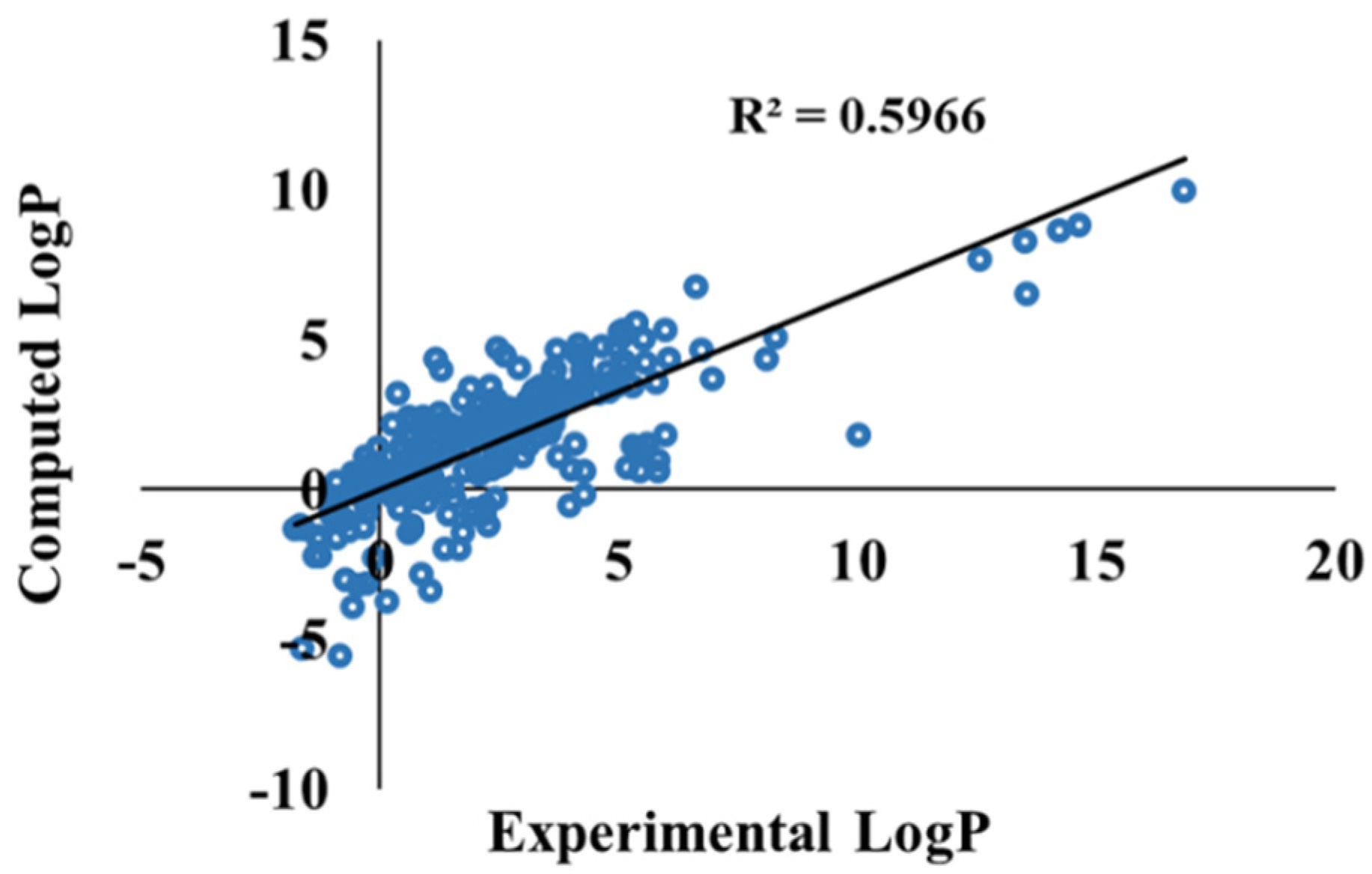
3.3. Ketone–Water Partition Coefficient Calculations Using the 3D-RISM-KH Theory

The ketone water partition coefficients were calculated by correcting the GF-solvation free energy calculated using the 3D-RISM-KH theory in respective solvent media. The regression coefficients for the hydration free energy calculation was obtained by benchmarking the hydration free energy computation against the experimental hydration free energies obtained from the FreeSolv database. For hydration free energy calculation, a MAD of 1.4 kcal/mol is obtained for 642 solutes. The details of these solutes are provided in the Supplementary Materials. The 3D-RISM-KH theory computed cyclohexanone–water partition coefficients of 29 solutes have MAD of 0.42 units. The partition coefficients for acyclic ketone-water partitioning with a higher MAD of ~1.3 units were obtained. The overall correlation between the experimental and computed ketone–water partition coefficients showed a good correlation (r² = 0.596) for a total of 284 solutes (Figure 2).

4. Discussion

In this work, we have first validated the force field parameters for four aliphatic ketones for use as solvents in the 3D-RISM-KH molecular solvation theory. The liquid states of three acyclic ketones (acetone, MEK, and MIBK) and one cyclic ketone (cyclohexanone) were modeled using united-atom force field parameters. The resultant XRISM-KH-based liquid profiles of these four ketones agree very well with the relevant features observed in the MD simulations with the all-atom force field. The liquid structures of the acyclic ketones differ significantly from the cyclic one. Several different local orientations of the molecules exist in the cyclohexane system, owing to the six-member ring framework. Both the MD and RISM calculations underscore these findings. Subsequently, the XRISM-KH-computed solvent susceptibility function is used to calculate the solvation free energy of small molecules with known experimental solvation free energies in different ketones studied here. Our result showed a very good performance of the 3D-RISM-KH-theory-based solvation free energy calculations in liquid ketones, with excellent accuracy at a very modest computational cost. Finally, we have compared the ketone–water partition coefficients for 284 organic molecules for which experimental partitioning coefficients were reported in the literature. Our results are in good agreement with the experimental results. We have noted comparatively large deviations in the calculations for the systems containing N/P/S atom(s), and further considerations should be made while choosing force field parameters for such a type of systems. The partition coefficients calculated for CYO-water and MEK-Water were found to be better than those computed for other two-ketone water systems. Tuning or modifying force field parameters may further help in better correlations with experiments. Further refinements of the ketone–water partition coefficient can be achieved by considering conformational flexibility of relatively larger systems via longer simulations.

References

1. Skyner, R.E.; McDonagh, J.L.; Groom, C.R.; van Mourika, T.; Mitchell, J.B.O. A review of methods for the calculation of solution free energies and the modelling of systems in solution. Phys. Chem. Chem. Phys. 2015, 17, 6174–6191. [Google Scholar] [CrossRef] [Green Version]
2. Matos, G.D.R.; Kyu, D.Y.; Loeffler, H.H.; Chodera, J.D.; Shirts, M.R.; Mobley, D.L. Approaches for calculating solvation free energies and enthalpies demonstrated with an update of the FreeSolv database. J. Chem. Eng. Data 2017, 62, 1559–1569. [Google Scholar] [CrossRef] [Green Version]
3. Mennucci, B. Polarizable continuum model. WIREs Comput. Mol. Sci. 2012, 2, 386–404. [Google Scholar] [CrossRef]
4. Tomasi, J.; Mennucci, B.; Cammi, R. Quantum Mechanical Continuum Solvation Models. Chem. Rev. 2005, 105, 2999–3094. [Google Scholar] [CrossRef]
5. Zhang, J.; Zhang, H.; Wu, T.; Wang, Q.; van der Spoel, D. Comparison of Implicit and Explicit Solvent Models for the Calculation of Solvation Free Energy in Organic Solvents. J. Chem. Theory Comput. 2017, 13, 1034–1043. [Google Scholar] [CrossRef]
6. Cramer, C.J.; Truhlar, D.G. Implicit Solvation Models: Equilibria, Structure, Spectra, and Dynamics. Chem. Rev. 1999, 99, 2161–2220. [Google Scholar] [CrossRef]
7. Pliego, J.R.; Riveros, J.M. The Cluster—Continuum Model for the Calculation of the Solvation Free Energy of Ionic Species. J. Phys. Chem. A 2001, 105, 7241–7247. [Google Scholar] [CrossRef]
8. Tomaník, L.; Muchová, E.; Slavíček, P. Solvation energies of ions with ensemble cluster-continuum approach. Phys. Chem. Chem. Phys. 2020, 22, 22357–22368. [Google Scholar] [CrossRef]
9. Roy, D.; Dutta, D.; Wishart, D.; Kovalenko, A. Predicting PAMPA permeability using the 3D-RISM-KH theory: Are we there yet? J. Comput.-Aided Mol. Des. 2021, 35, 261–269. [Google Scholar] [CrossRef]
10. Roy, D.; Hinge, V.K.; Kovalenko, A. To Pass or Not to Pass: Predicting the Blood—Brain Barrier Permeability with the 3D-RISM-KH Molecular Solvation Theory. ACS Omega 2019, 4, 16774–16780. [Google Scholar] [CrossRef]
11. Hinge, V.K.; Blinov, N.; Roy, D.; Wishart, D.; Kovalenko, A. The role of hydration effects in 5-fluorouridine binding to SOD1: Insight from a new 3D-RISM-KH based protocol for including structural water in docking simulations. J. Comput.-Aided Mol. Des. 2019, 33, 913–926. [Google Scholar] [CrossRef]
12. Omelyan, I.; Kovalenko, A. MTS-MD of Biomolecules Steered with 3D-RISM-KH Mean Solvation Forces Accelerated with Generalized Solvation Force Extrapolation. J. Chem. Theory Comput. 2015, 11, 1875–1895. [Google Scholar] [CrossRef]
13. Imai, T.; Oda, K.; Kovalenko, A.; Hirata, F.; Kidera, A. Ligand Mapping on Protein Surfaces by the 3D-RISM Theory: Toward Computational Fragment-Based Drug Design. J. Am. Chem. Soc. 2009, 131, 12430–12440. [Google Scholar] [CrossRef]
14. Sugita, M.; Hamano, M.; Kasahara, K.; Kikuchi, T.; Hirata, F. New Protocol for Predicting the Ligand-Binding Site and Mode Based on the 3D-RISM/KH Theory. J. Chem. Theory Comput. 2020, 16, 2864–2876. [Google Scholar] [CrossRef]
15. Sindhikara, D.J.; Hirata, F. Analysis of Biomolecular Solvation Sites by 3D-RISM Theory. J. Phys. Chem. B 2013, 117, 6718–6723. [Google Scholar] [CrossRef]
16. Truchon, J.-F.; Pettitt, B.M.; Labute, P. A Cavity Corrected 3D-RISM Functional for Accurate Solvation Free Energies. J. Chem. Theory Comput. 2014, 10, 934–941. [Google Scholar] [CrossRef]
17. Misin, M.; Fedorov, M.V.; Palmer, D.S. Communication: Accurate hydration free energies at a wide range of temperatures from 3D-RISM. J. Chem. Phys. 2015, 142, 091105. [Google Scholar] [CrossRef] [Green Version]
18. Gavazzoni, C.; Skaf, M.S. Adsorption of CO2 and CH4 in MIL-47 investigated by the 3D-RISM molecular theory of solvation. Phys. Chem. Chem. Phys. 2020, 22, 13240–13247. [Google Scholar] [CrossRef]
19. Genheden, S.; Luchko, T.; Gusarov, S.; Kovalenko, A.; Ryde, U. An MM/3D-RISM approach for ligand binding affinities. J. Phys. Chem. B 2010, 114, 8505–8516. [Google Scholar] [CrossRef]
20. Kaminski, J.W.; Gusarov, S.; Wesolowski, T.A.; Kovalenko, A. Modeling Solvatochromic Shifts Using the Orbital-Free Embedding Potential at Statistically Mechanically Averaged Solvent Density. J. Phys. Chem. A 2010, 114, 6082–6096. [Google Scholar] [CrossRef]
21. Chandler, D.; McCoy, J.D.; Singer, S.J. Density functional theory of nonuniform polyatomic systems. I. General formulation. J. Chem. Phys. 1986, 85, 5971–5976. [Google Scholar] [CrossRef]
22. Chandler, D.; McCoy, J.D.; Singer, S.J. Density functional theory of nonuniform polyatomic systems. II. Rational closures for integral equations. J. Chem. Phys. 1986, 85, 5977–5982. [Google Scholar] [CrossRef]
23. Lowden, L.J.; Chandler, D. Solution of a new integral equation for pair correlation functions in molecular liquids. J. Chem. Phys. 1973, 59, 6587–6595. [Google Scholar] [CrossRef]
24. Chandler, D. Cluster diagrammatic analysis of the RISM equation. Mol. Phys. 1976, 31, 1213–1223. [Google Scholar] [CrossRef]
25. Andersen, H.C.; Chandler, D.; Weeks, J.D. Roles of repulsive and attractive forces in liquids, the equilibrium theory of classical fluids. Adv. Chem. Phys. 1976, 34, 105–155. [Google Scholar]
26. Kovalenko, A. Molecular theory of solvation: Methodology summary and illustrations. Cond. Matt. Phys. 2015, 18, 32601. [Google Scholar] [CrossRef] [Green Version]
27. Kovalenko, A. Multiscale Modeling of Solvation. In Springer Handbook of Electro-Chemical Energy; Breitkopf, C., Swider-Lyons, K., Eds.; Springer: Berlin/Heidelberg, Germany, 2017. [Google Scholar]
28. Kovalenko, A.; Gusarov, S. Multiscale methods framework: Self-consistent coupling of molecular theory of solvation with quantum chemistry, molecular simulations, and dissipative particle dynamics. Phys. Chem. Chem. Phys. 2017, 20, 2947–2969. [Google Scholar] [CrossRef]
29. Ratkova, E.L.; Palmer, D.S.; Fedorov, M.V. Solvation Thermodynamics of Organic Molecules by the Molecular Integral Equation Theory: Approaching Chemical Accuracy. Chem. Rev. 2015, 13, 6312–6356. [Google Scholar] [CrossRef] [Green Version]
30. Kovalenko, A.; Hirata, F. A molecular theory of liquid interfaces. Phys. Chem. Chem. Phys. 2005, 7, 1785–1793. [Google Scholar] [CrossRef]
31. Palmer, D.S.; Frolov, A.; Ratkova, E.; Fedorov, M.V. Towards a universal method for calculating hydration free energies: A 3D reference interaction site model with partial molar volume correction. J. Phys. Condens. Matt. 2010, 22, 492101. [Google Scholar] [CrossRef]
32. Zhao, Y.; Truhlar, D.G. The M06 suite of density functionals for main group thermochemistry, thermochemical kinetics, noncovalent interactions, excited states, and transition elements: Two new functionals and systematic testing of four M06-class functionals and 12 other functionals. Theor. Chem. Acc. 2008, 120, 215–241. [Google Scholar]
33. Weigend, F.; Ahlrichs, R. Balanced basis sets of split valence, triple zeta valence and quadruple zeta valence quality for H to Rn: Design and assessment of accuracy. Phys. Chem. Chem. Phys. 2005, 7, 3297–3305. [Google Scholar] [CrossRef]
34. Tomasi, J.; Mennucci, B.; Cancès, E. The IEF version of the PCM solvation method: An overview of a new method addressed to study molecular solutes at the QM ab initio level. J. Mol. Struct. (Theochem) 1999, 464, 211–226. [Google Scholar] [CrossRef]
35. Barone, V.; Cossi, M.; Tomasi, J. A new definition of cavities for the computation of solvation free energies by the polarizable continuum model. J. Chem. Phys. 1997, 107, 3210–3221. [Google Scholar] [CrossRef]
36. Marenich, A.V.; Cramer, C.J.; Truhlar, D.G. Universal solvation model based on solute electron density and a continuum model of the solvent defined by the bulk dielectric constant and atomic surface tensions. J. Phys. Chem. B 2009, 113, 6378–6396. [Google Scholar] [CrossRef]
37. Frisch, M.J.; Trucks, G.W.; Schlegel, H.B.; Scuseria, G.E.; Robb, M.A.; Cheeseman, J.R.; Scalmani, G.; Barone, V.; Petersson, G.A.; Nakatsuji, H.; et al. Gaussian 16, Revision B.01; Gaussian, Inc.: Wallingford, CT, USA, 2016. [Google Scholar]
38. Abraham, M.J.; Murtola, T.; Schulz, R.; Páll, S.; Smith, J.C.; Hess, B.; Lindahl, E. GROMACS: High performance molecular simulations through multi-level parallelism from laptops to supercomputers. SoftwareX 2015, 1–2, 19–25. [Google Scholar] [CrossRef] [Green Version]
39. Wang, J.; Wang, W.; Kollman, P.A.; Case, D.A. Automatic atom type and bond type perception in molecular mechanical calculations. J. Mol. Graph. Model. 2006, 25, 247260. [Google Scholar] [CrossRef]
40. Jakalian, A.; Jack, D.B.; Bayly, C.I. Fast, efficient generation of high-quality atomic charges. AM1-BCC model: II. Parameter-ization and validation. J. Comput. Chem. 2002, 23, 1623–1641. [Google Scholar] [CrossRef]
41. Jorgensen, W.L.; Madura, J.D.; Swenson, C.J. Optimized intermolecular potential functions for liquid hydrocarbons. J. Am. Chem. Soc. 1984, 106, 6638. [Google Scholar] [CrossRef]
42. Kobryn, A.E.; Kovalenko, A. Molecular theory of hydrodynamic boundary conditions in nanofluidics. J. Chem. Phys. 2008, 129, 134701. [Google Scholar] [CrossRef] [PubMed]
43. Møller, C.; Plesset, M.S. Note on an approximation treatment for many-electron systems. Phys. Rev. 1934, 46, 618–622. [Google Scholar] [CrossRef] [Green Version]
44. Head-Gordon, M.; Head-Gordon, T. Analytic MP2 Frequencies without Fifth Order Storage: Theory and Application to Bifurcated Hydrogen Bonds in the Water Hexamer. Chem. Phys. Lett. 1994, 220, 122–128. [Google Scholar] [CrossRef]
45. Luchko, T.; Blinov, N.; Limon, G.C.; Joyce, K.P.; Kovalenko, A. SAMPL5: 3D-RISM partition coefficient calculations with partial molar volume corrections and solute conformational sampling. J. Comput.-Aided Mol. Des. 2016, 30, 1115–1127. [Google Scholar] [CrossRef] [PubMed]
46. O’Boyle, N.M.; Banck, M.; James, C.A.; Morley, C.; Vandermeersch, T.; Hutchison, G.R. Open Babel: An open chemical toolbox. J. Cheminfo. 2011, 3, 33. [Google Scholar] [CrossRef] [PubMed] [Green Version]
47. Halgren, T.A. Merck molecular force field. I. Basis, form, scope, parameterization, and performance of MMFF94. J. Comput. Chem. 1996, 17, 490–519. [Google Scholar] [CrossRef]
48. Marenich, A.V.; Kelly, C.P.; Thompson, J.D.; Hawkins, G.D.; Chambers, C.C.; Giesen, D.J.; Winget, P.; Cramer, C.J.; Truhlar, D.G. Minnesota Solvation Database (MNSOL) Version 2012; University of Minnesota: Minneapolis, MN, USA, 2012. [Google Scholar]
49. Michael, H.; Abraham, M.H.; Acree, W.E.; Leoc, A.J.; Hoekmand, D. The partition of compounds from water and from air into wet and dry ketones. New J. Chem. 2009, 33, 568–573. [Google Scholar]
50. Mobley, D.L.; Guthire, P. FreeSolv: A database of experimental and calculated hydration free energies, with input files. J. Comput.-Aided Mol. Des. 2014, 28, 711–720. [Google Scholar] [CrossRef] [Green Version]
Figure 1. Radial distribution functions obtained from the all-atom MD simulations (left panels) and the 3D-RISM-KH calculations (right panels).
J 04 00044 g001
Figure 2. Correlation between experimental and 3D-RISM-KH computed ketone–water partition coefficients.
J 04 00044 g002