Nonparametric Conditional Heteroscedastic Hourly Probabilistic Forecasting of Solar Radiation


Centre for Industrial and Applied Mathematics, School of ITMS, University of South Australia, Mawson Lakes 5095, Australia
*
Author to whom correspondence should be addressed.
†
These authors contributed equally to this work.
J 2018, 1(1), 174-191; https://doi.org/10.3390/j1010016
Submission received: 26 October 2018
/
Revised: 17 November 2018
/
Accepted: 29 November 2018
/
Published: 4 December 2018
(This article belongs to the Special Issue Feature Papers for J-Multidisciplinary Scientific Journal)
Abstract
:We develop a new probabilistic forecasting method for global horizontal irradiation (GHI) by extending our previous bootstrap method to a case of an exponentially decaying heteroscedastic model for tracking dynamics in solar radiance. Our previous method catered for the global systematic variation in variance of solar radiation, whereas our new method also caters for the local variation in variance. We test the performance of our new probabilistic forecasting method against our old probabilistic forecasting method at three locations: Adelaide, Darwin, and Mildura. These locations are chosen to represent three distinct climates. The prediction interval coverage probability, prediction interval normalized averaged width and Winkler score results from our new probabilistic forecasting method are encouraging. Our new method performs better than our previous method at Adelaide and Mildura; regions with a higher proportion of clear-sky days, whereas our previous method performs better than our new method at Darwin; a region with a lower proportion of clear-sky days. These results suggest that the ideal probabilistic forecasting method might be climate specific.
1. Introduction
When supplying energy into the electricity grid, it is important to know the expected output from solar energy systems. While a point forecast of the expected output is valuable, it is only the expected value, whereas a probabilistic forecast gives a range of the most likely values of the output. A probabilistic forecast provides information about all expected outputs and allows one to asses a wide range of uncertainties and that can in turn improve decision making. A probabilistic forecast can be thought of as the error bounds of the forecast. These error bounds are also known as prediction intervals.
Probabilistic forecasting is becoming more prevalent in the renewable energy forecasting literature. Note also that one of the priorities of the International Energy Agency Task 16 on “Solar resource for high penetration and large-scale applications” is developing the best methods for probabilistic forecasting of solar radiation. For a detailed literature review on probabilistic forecasting, please refer to our earlier work [1] on probabilistic forecasting of solar irradiation. Since then, several studies have been reported in the literature. Please note that a glossary describing the symbols used is given at the end of the paper in Section 6.
Lauret et al. [2] develop three probabilistic forecasts based on nonparametric methods of linear quantile regression. Scolari et al. [3] develop ultra-short-term (from 500-millisecond to 5-min) probabilistic forecasts of global horizontal irradiance. They use a nonparametric method based on k-means clustering of historical data according to certain influential variables; average clear-sky index and clear-sky index variability. Chu and Coimbra [4] develop very short-term (5-, 10-, 15- and 20-min) probabilistic forecasts of direct normal irradiance (DNI) based on a k-nearest neighbor ensemble (kNNEn) method. An assessment of machine learning techniques for intra-hour point and probabilistic forecasting is performed by [5].
David et al. [6] develop probabilistic forecasts on time scales of ten minutes to six hours of global horizontal irradiance. They use a clear-sky model to model the annual and diurnal cycles and a combination of the auto regressive moving average (ARMA) model to describe the serial correlation and the parametric generalized auto regressive conditional heteroscedasticity (GARCH) model to model the volatility.
Trapero [7] develops one-step-ahead hourly uncertainty forecasts of global horizontal irradiation (GHI) using kernel density estimates, GARCH and Single Exponential Smoothing methods, and a combination of the before mentioned methods. They find that the combination of methods is a good compromise between coverage and interval width.
Voyant et al. [8] uses two persistent and four machine learning point forecasting methods for one-step-ahead hourly GHI. The probabilistic forecast (one to six hours) method is based on the bootstrap sampling of a training set using the k-fold method, together with the cumulative distribution function (CDF).
It is important to note that most of the studies in the literature use a clear-sky model to encapsulate the climatology (de-trending) of GHI. We instead use Fourier series to model the climatology.
In this paper, we develop a new probabilistic forecasting method. Our new probabilistic forecasting method extends our previous bootstrap method [1,9] to a case of an exponentially decaying heteroscedastic model for tracking dynamics in solar radiance. For the remainder of this paper we refer to our old method as unconditional and our new method as conditional. The unconditional method catered for the global systematic variation in variance of solar radiation, whereas the conditional method also caters for the local variation in variance—in other words the conditional heteroscedastic nature. One could say that the unconditional picks up the climate variation in variance, while the conditional picks up the variation because of the weather. The performance of the unconditional method was very good, except in one aspect. Since the prediction interval construction was based solely on bootstrapping errors for the particular time of day and year, the present weather conditions were not taken into account. Thus, on a systematically clear day, the prediction intervals, although they exhibited the correct coverage criteria, they were much wider, less sharp, than one would hope. The conditional method presented here takes into account the conditions on the day as well as the time of day and year, and thus the intervals are sharper. Please note that even though the analysis is performed on hourly data similar procedures can be used for shorter time scales. In particular, they will be adapted to be used for forecasting output on a five-minute time scale for solar farms in Australia, under an Australian Renewable Energy Agency (ARENA) funded grant.
Boland and Soubdhan [10] use Fourier series for the climate variation, and then an autoregressive model to forecast the residual series after removal of the seasonal component. In that paper prediction intervals are formed for the forecasts at the three sites studied using an ARCH model technique. However, they do not take into account the interplay of systematic and conditional changes in variance that is integral to the treatment here.
This paper is organized as follows. A description of the data is given in Section 2. Section 3 describes both the point forecasting model and its performance. In Section 4 we describe our conditional probabilistic forecasting method, and report on its performance and compare the results to the literature in Section 5. The paper is concluded with a discussion of our findings and ideas for future work in Section 6.
2. Data and Preliminaries
Observed hourly GHI was obtained from the Australian Bureau of Meteorology [11] for three locations: Adelaide, Darwin, and Mildura. The three locations have three different climate types. We chose different climate types to determine how sensitive our methods might be to location.
Each data set consists of ten years of hourly GHI values with units of watt-hours per square meter, Wh·m. The first eight years were used for generating the point forecasting and probabilistic forecasting models (in-sample). The last two years were used for out-of-sample testing. Observations on 29 February in leap years were omitted. The Adelaide data set contains 1803 missing hourly GHI values and these were omitted.
3. Point Forecast
We begin with a description of our one-step-ahead point forecasting model. We use Fourier analysis to account for the seasonality and an autoregressive model to account for the serial correlation. Our hourly GHI model for Mildura is given by:
where is a seasonal component, is an autoregressive component, and is a noise such that , if and . That is, may be heteroscedastic. The autoregressive component is a linear combination of previous time steps.
We use power spectrum analysis to identify the significant frequencies in the Fourier component . We use 11 significant frequencies at cycles 1, 2, 364, 365, 366, 729, 730, 731, 1094, 1095 and 1096 cycles per year. These correspond to once-a-year (1) and twice-a-year (2) cycles, once-a-day (365), twice-a-day (730) and three-times-a-day cycles (1095), as well as the beat frequencies for the once-a-day (364, 366), twice-a-day (739, 731) and three-times-a-day cycles (1094, 1096). As [12] points out, the beat frequencies, also known as sidebands, are used to modulate the amplitude to suit the time of year. For our three locations, explains between 80–85% of the total variance.
We then use an autoregressive model of order 3, AR(3), to model the serial structure in the residuals after has been removed. The final step was to zero any night time values; solar altitudes less than zero degrees.
Similar point forecasting models were also developed for Adelaide and Darwin but are not shown here. For a detailed description of our point forecasting method, the reader is encouraged to read our previous paper [1].
Point Forecast Performance Evaluation
Table 2 shows the out-of-sample normalized root means square error (NRMSE), mean bias error (MBE) and mean absolute error (MAE) for the point forecasting method for Adelaide, Darwin, and Mildura. The NRMSE is normalized using the mean daytime value. With an adequately performing one-step-ahead point forecast, the next step is to develop a probabilistic forecast. It is not our intent here to compare our point forecasting model to a smart persistence model, as is commonly done in the literature, as we did this in our previous paper [1] and showed our method’s superior performance. In addition, our proposed methodology for generating a probabilistic forecast can be extended to other point forecasting methods, such as those proposed in, for example, [12,13,14] and the references therein.
4. Probabilistic Forecasting
We previously developed a computationally efficient and data-driven method for short-term probabilistic forecasting of solar radiation, using a nonparametric bootstrapping method and a map of sun positions [1]. The idea behind using this method was to account for the heteroscedasticity of the white noise in Equation (1).
The hourly daytime errors (noise) from the in-sample forecast are placed into a two-dimensional array according to the sun position (determined by sun elevation and solar hour angle), for a given hour. The rows i correspond to sun elevations in increments of ten degrees and the columns j correspond to solar hour angles in increments of fifteen degrees. We did this to take care of the systematic variation in variance in the GHI time series. That is, the variance in GHI differs throughout the day (higher in the middle of the day compared to the beginning and end of the day) and throughout the year (higher in summer compared to winter). The result is a two-dimensional array, where each element is a bin of errors corresponding to a specific sun position.
We generate prediction intervals using nonparametric resampling (with replacement). To generate a prediction interval for a particular hour, the empirical - and -quantiles from the bin in the two-dimensional array corresponding to the sun position for the hour are calculated. The empirical - and -quantiles are then added to the point forecast , resulting in lower and upper prediction intervals for the hour. Our method develops prediction intervals without imposing any parametric assumptions on the underlying distribution of GHI. As an example, suppose we wish to construct 95% prediction intervals for our forecasts. We first determine, given the time of day and day of the year, which bin the forecast is referring to, and use the error distribution in that bin for our calculations. For this error distribution we determine the 2.5% and 97.5% quantiles for this empirical distribution. We then add these values to the forecasted value of the solar irradiation determined by the point forecast method to construct our prediction interval.
For a detailed description of our previous probabilistic forecasting method, the reader is encouraged to consult our previous paper [1].
The conditional method for generating a probabilistic forecast described in this paper, extends our unconditional method to a case of an exponentially decaying heteroscedastic model for tracking dynamics in solar radiance. The unconditional method catered for the global systematic variation in variance of solar radiation, whereas the conditional method also caters for the local variation in variance.
The problem with the unconditional method is that while it caters for the variance GHI can exhibit for a particular time of year/time of day (global), it does not cater for the variance in GHI that is currently evident at time t (local). The conditional method also takes into the account the current variance. For example, if the current variance at time t is small, then the conditional method will generate prediction intervals for time t + 1 that are narrower than otherwise would be generated by the unconditional method.
The final errors are uncorrelated but dependent. Uncorrelated refers to the fact that the means at each time step are not connected, but the series can still be dependent since dependence between the variances remains. This is exemplified by the squared error terms, a proxy for variance, being correlated. This characteristic is the so-called autoregressive conditional heteroscedastic (ARCH) effect. Usually when this happens one uses an ARCH or GARCH model for forecasting the variance.
However, we found that instead an exponential smoothing form performed better than an ARCH or GARCH model:
where is the variance at time t.
Since we are forecasting the variance, and then constructing a prediction interval using this forecast, we must perform the forecast assuming the noise is normally distributed, which is not true. Therefore, we first had to use a normalizing transformation, then forecast the variance, construct the prediction intervals, and then transform back. Templeton [15] describes a method for transforming a non-normal variable to normal. In each bin of errors, we have distributions that are non-normal. We transform the errors to normal for each bin independently. We first find for each error its percent rank, in other words how far along the empirical CDF it lies. The result is uniformly distributed probabilities. We then apply the inverse normal transformation to these probabilities, resulting in values from the standard normal distribution. We can then use these squared normal errors as proxies for the variance and proceed to construct a forecast model.
The method for generating the lower and upper prediction intervals is shown in Algorithm 1.
The final step in generating prediction intervals is to impose sensible upper and lower limits. We impose a lower bound limit of zero on the lower prediction interval. We restrict the upper prediction interval using the Bird clear-sky model [16] and then add twenty percent for cloud enhancement [17].
Figure 2, Figure 3 and Figure 4 compares 95% prediction intervals using the unconditional and conditional probabilistic forecasting methods, for clear and cloudy days, for Adelaide, Darwin, and Mildura respectively. A clear-sky day is where there is little evidence of the transient effects of clouds causing no fluctuations in GHI. A cloudy day is where there is some evidence of the transient effects of clouds causing fluctuations in GHI.
| Algorithm 1: Algorithm for generating (100-) prediction intervals using the conditional method. |
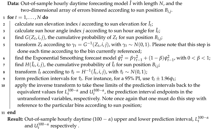 |
For clear-sky days, the observed GHI values fall within the prediction intervals with unconditional probabilistic forecasting method providing narrower prediction intervals for all three locations. For cloudy days, most of the observed GHI values fall within the prediction intervals with the conditional probabilistic forecasting method providing narrower prediction intervals for all three locations. In the next section we numerically examine the performance of our conditional probabilistic forecasting method.
5. Probabilistic Forecast Performance Evaluation
In line with the broader probabilistic forecasting and prediction interval literature [3,18,19,20], we use three standard performance metrics: prediction interval coverage probability (PICP), prediction interval normalized averaged width (PINAW) and Winkler score. We do not include performance measurements of rank histograms or continuous rank probability score because we do not generate an ensemble forecast. As described in Section 4, we generate prediction intervals by forecasting the variance using empirical quantiles from each bin in . We also do not use the coverage width-based criterion (CWC) because we share the same concerns as [21]. They suggest that the CWC may give a better score to intervals that are actually of lower quality.
5.1. Prediction Interval Coverage Probability
The PICP is the percentage of times an observation falls within the prediction intervals for a nominal prediction interval. A probabilistic forecast is considered calibrated if the PICP is close to the nominal value. For example, the ideal PICP for a 95% prediction interval is 95%. The PICP for a nominal prediction interval is given by:
where L is the total number of forecasts and
and is the observed GHI value.
Figure 5 shows the reliability of the prediction intervals in the form of quantile–quantile plots [22,23] over the out-of-sample period, using the conditional and unconditional probabilistic forecasting methods, for Adelaide, Darwin, and Mildura. That is, each subfigure shows the PICP vs. the expected nominal coverage. These diagrams are known in the literature as reliability diagrams. For a calibrated probabilistic forecasting method, the PICP should follow a strong linear relationship with the nominal coverage rates by falling within the 95% consistency bars [24,25,26] along the 45-degree black reference line. For Adelaide and Mildura, the PICP for both probabilistic forecasting methods fall within or just outside the consistency bars, with the conditional probabilistic forecasting method performing slightly better. For Darwin, the PICP for the unconditional forecasting method falls outside the consistency bars but inside for the conditional method. Overall, the results show that our conditional probabilistic forecasting method is calibrated.
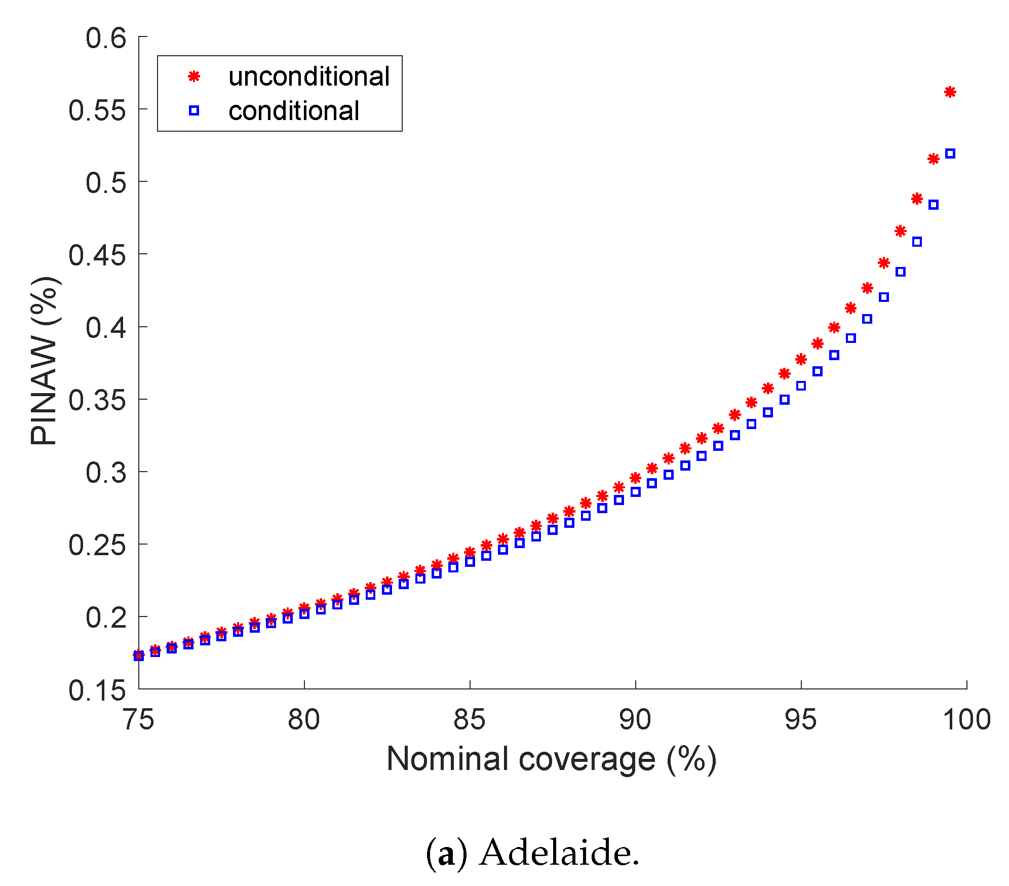
5.2. Prediction Interval Normalized Averaged Width
While we want a calibrated probabilistic forecast, we also want a sharp probabilistic forecast with narrow prediction intervals. To measure prediction interval width, we use PINAW:
where = 1000 Wh·m.
Figure 6 shows the PINAW for all nominal prediction intervals, over the out-of-sample period, for the unconditional and conditional probabilistic forecasting methods, for Adelaide, Darwin, and Mildura. The results are mixed. The prediction intervals are only sharper using the conditional forecasting method for Adelaide and Mildura.
5.3. Winkler Score
Coverage and prediction interval widths are isomorphic. Because coverage is easily obtained by having wider prediction interval widths over the out-of-sample period 2013–2014, we examine the trade-off between coverage and prediction interval width using the Winkler score [20], proposed by [27]. The Winkler score is defined as:
We normalize the Winkler score by dividing it by the total GHI value. A better performing prediction interval is characterized by a lower Winkler score.
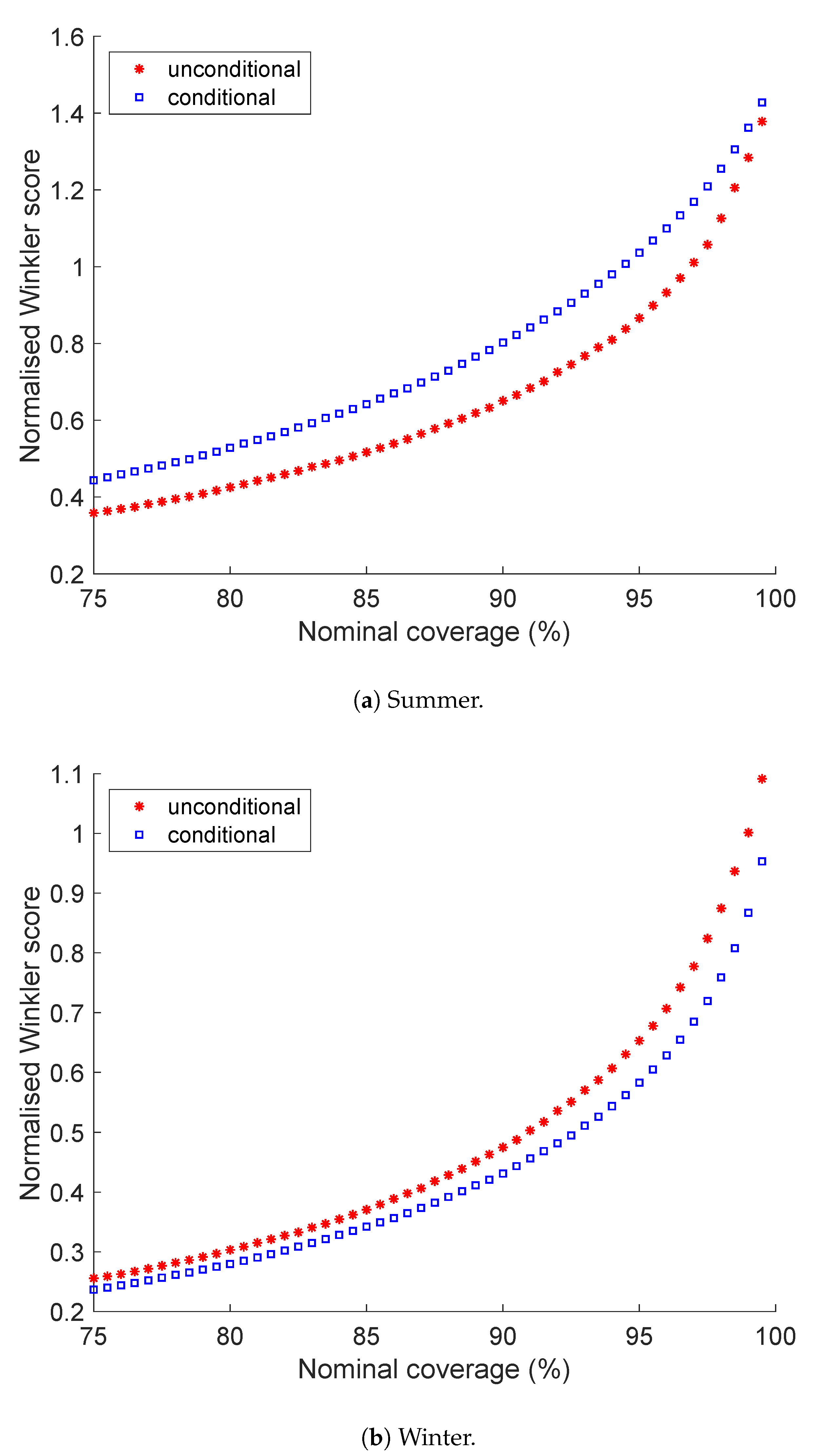
Figure 7 shows the normalized Winkler score for all nominal prediction intervals over the out-of-sample period, for the unconditional and conditional probabilistic forecasts, for Adelaide, Darwin, and Mildura, respectively.
These figures show the conditional probabilistic forecasting method performs better than the unconditional probabilistic forecasting method for Adelaide and Mildura. Interestingly, this observation is not the case for Darwin. We examine Darwin more closely in Section 5.4.
5.4. A Closer Look at Darwin
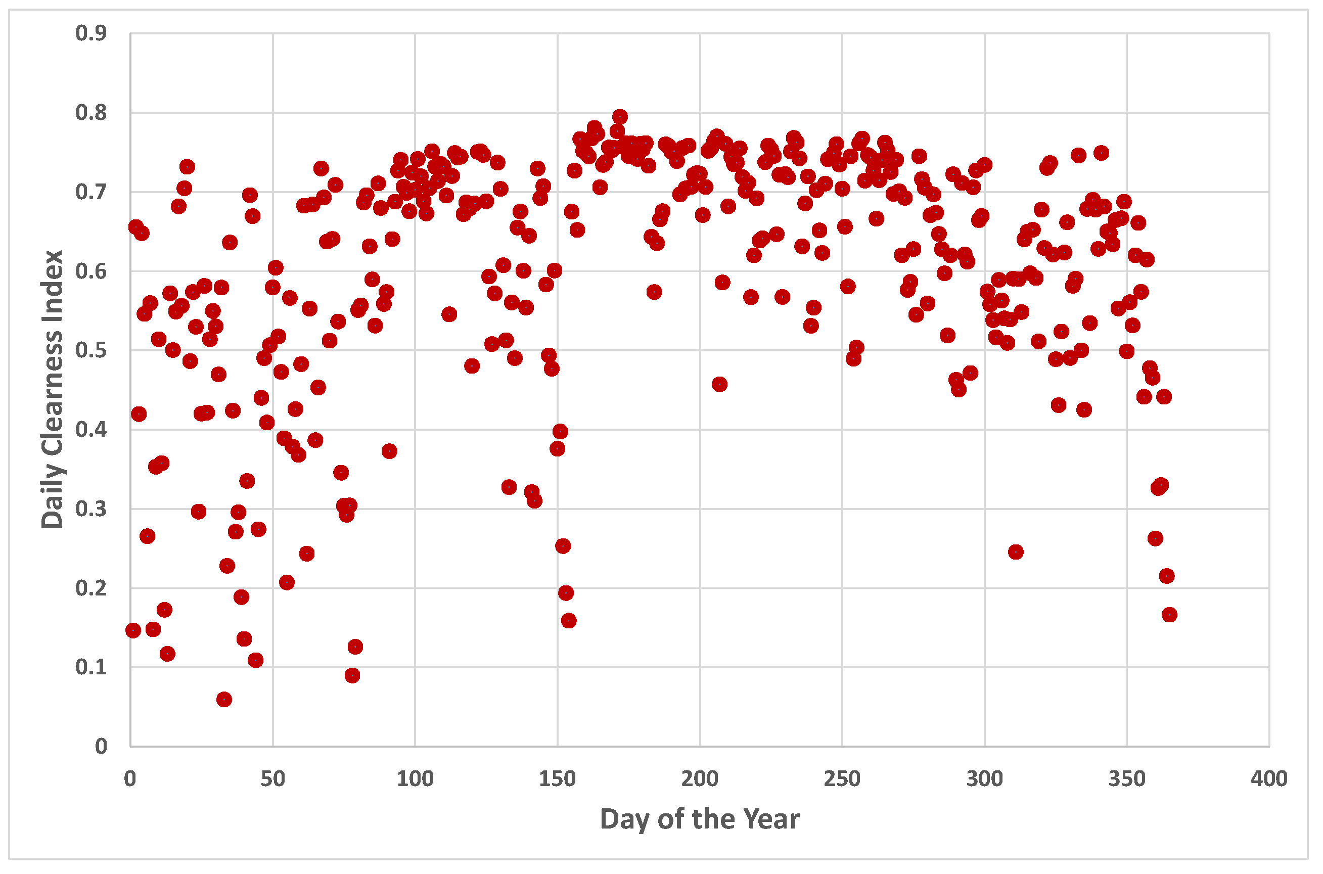
According to the Köppen-Geiger climate classification system, Darwin’s climate is classified as Tropical, with distinct dry and wet seasons. Perhaps the performance of the probabilistic forecasting methods is dependent upon the season. Figure 8 shows the daily clearness index for Adelaide and Figure 9 for Darwin, for one year. We can see that the variability of clearness index for Adelaide appears to be constant over the year. A similar case for Mildura (not shown here). However, for Darwin, there appears to be a greater variability of clearness index during the summer months (wet season) compared to the winter months (dry season). Therefore, we break our analysis down into these two seasons. We define summer as the months November to May and winter months as June to October.
Figure 10 shows the reliability of the prediction intervals in the form of quantile–quantile plots [22,23] over the out-of-sample period, using the unconditional and conditional probabilistic forecasting methods, for Darwin, for summer and winter. The reliability of conditional probabilistic forecasting method performs well for both summer and winter months. However, the unconditional probabilistic forecasting method markedly under covers during the summer months and over covers during the winter months, particularly for lower nominal coverage rates.
Figure 11 shows the normalized Winkler score for all nominal prediction intervals over the out-of-sample period 2013–2014, for the unconditional and conditional combinations probabilistic forecasts, for Darwin, for summer and winter.
Based on the lower normalized Winkler scores, one might suggest using the unconditional probabilistic forecasting method for summer months and the conditional probabilistic forecasting method during the winter months. However, as Figure 10 shows, it would come at the cost of coverage during winter which is not a desired result. That is, there is no point in having narrow prediction intervals if there is no coverage.
5.5. Results in the Literature
In this section, we compare our method to similar methods in the literature. Where applicable, we believe our conditional probabilistic forecasting method performs well compared to other methods.
Unfortunately, it is not clear what the nominal prediction intervals are in [8]. Therefore, we do not make a comparison.
David et al. [6] do not report on prediction interval widths but do provide reliability diagrams that shows the PICP. However, as they acknowledge, the coverage of their probabilistic forecasts do not match the nominal prediction intervals for all coverage probabilities—with deviations away from the ideal line.
Pedro et al. [5] reports on the PICP and PINAW metrics for time scales up to thirty minutes. The results from their reliability diagrams are mixed with deviations from the ideal line for some methods. They provide PINAW results for 80% prediction intervals with the best performing method scoring 9.9%. Our best performing location, Mildura, scored 16.4%. It is important to note that our time scale is hourly, not thirty minutes, so a higher percentage is expected.
Trapero [7] have well calibrated prediction intervals for their combined method with the PICPs matching the nominal coverages. To measure how sharp their probabilistic forecast is, they do not use the PINAW metric. Instead they use the average interval width metric which is calculated by dividing the interval range by its midpoint. For their combined method for a nominal coverage of 95%, the average width is 1.32. For a nominal coverage of 95% for Mildura, we used their average interval width metric and our conditional method scored 0.79.
6. Conclusions
In the paper we have described our new conditional probabilistic forecasting method which extends our old unconditional method to a case where we cater for the heteroscedastic nature of the series by constructing an exponentially weighted smoothing average model for forecasting the variance. The conditional method caters for both the global systematic variation in variance of solar radiation and the local variation in variance. Results show that the conditional method performs better than the unconditional method for locations exhibiting more clear-sky days, while results are mixed for the location with less clear-sky days. It could be that this would be improved if the point forecast model were to be developed separately for the different seasons for locations such as Darwin with pronounced differences in cloud cover in different seasons. Results also show our method compares well to the literature.
Future work will examine if there is an optimal way of combining the two probabilistic forecasting methods, perhaps using gradient boosting. We would also like to incorporate a numerical weather prediction (NWP) forecast into our point forecast to see if this improves performance of both the point forecast as well as the probabilistic forecast.
Author Contributions
Conceptualization, J.B. and A.G.; Methodology, J.B. and A.G.; Software, J.B. and A.G.; Validation, J.B. and A.G.; Formal Analysis, J.B. and A.G.; Investigation, J.B. and A.G.; Resources, J.B. and A.G.; Data Curation, J.B. and A.G.; Writing-Original Draft Preparation, J.B. and A.G.; Writing-Review & Editing, J.B. and A.G.; Visualization, J.B. and A.G.; Supervision, J.B.; Funding Acquisition, J.B. and A.G.
Funding
This research is partly funded by an Australian Mathematical Society Lift-off Fellowship. The authors would also like to acknowledge the Australian Mathematical Society for their support of the project.
Conflicts of Interest
The authors declare no conflict of interest.
Glossary
| hourly solar irradiation | |
| seasonal component of the solar irradiation | |
| autoregressive component of the solar irradiation | |
| noise term for the solar forecast model | |
| two-dimensional array for binning the noise, according to the sun position | |
| i corresponds to the sun elevation and j to the sun hour angle | |
| variance of the noise term at time t | |
| exponential smoothing parameter | |
| forecast of at time | |
| transformation of to the corresponding value in probability in | |
| transformation of to the corresponding value in probability in | |
| empirical cumulative distribution function of the noise term | |
| empirical cumulative distribution function of the solar forecast | |
| lower bound of the prediction interval | |
| upper bound of the prediction interval | |
| probability level for determining the prediction interval. For example, for a 95% prediction interval, | |
| the width of the prediction interval at time t |
References
- Grantham, A.; Gel, Y.R.; Boland, J. ScienceDirect Nonparametric short-term probabilistic forecasting for solar radiation. Sol. Energy 2016, 133, 465–475. [Google Scholar] [CrossRef]
- Lauret, P.; David, M.; Pedro, H.T.C. Probabilistic Solar Forecasting Using Quantile Regression Models. Energies 2017, 10, 1591. [Google Scholar] [CrossRef]
- Scolari, E.; Sossan, F.; Paolone, M. Irradiance prediction intervals for {PV} stochastic generation in microgrid applications. Sol. Energy 2016, 139, 116–129. [Google Scholar] [CrossRef]
- Chu, Y.; Coimbra, C.F.M. Short-term probabilistic forecasts for Direct Normal Irradiance. Renew. Energy 2017, 101, 526–536. [Google Scholar] [CrossRef]
- Pedro, H.T.; Coimbra, C.F.; David, M.; Lauret, P. Assessment of machine learning techniques for deterministic and probabilistic intra-hour solar forecasts. Renew. Energy 2018, 123, 191–203. [Google Scholar] [CrossRef]
- David, M.; Ramahatana, F.; Trombe, P.; Lauret, P. Probabilistic forecasting of the solar irradiance with recursive ARMA and GARCH models. Sol. Energy 2016, 133, 55–72. [Google Scholar] [CrossRef] [Green Version]
- Trapero, J.R. Calculation of solar irradiation prediction intervals combining volatility and kernel density estimates. Energy 2016, 114, 266–274. [Google Scholar] [CrossRef]
- Voyant, C.; Motte, F.; Notton, G.; Fouilloy, A.; Nivet, M.L.; Duchaud, J.L. Prediction intervals for global solar irradiation forecasting using regression trees methods. Renew. Energy 2018, 126, 332–340. [Google Scholar] [CrossRef] [Green Version]
- Grantham, A.; Pudney, P.; Boland, J. Generating synthetic sequences of global horizontal irradiation. Sol. Energy 2018, 162. [Google Scholar] [CrossRef]
- Boland, J.; Soubdhan, T. Spatial-temporal forecasting of solar radiation. Renew. Energy 2015, 75, 607–616. [Google Scholar] [CrossRef]
- Bureau of Meteorology. 2013. Available online: http://www.bom.gov.au/ (accessed on 3 December 2018).
- Boland, J.W. Time Series Modelling of Solar Radiation. In Modeling Solar Radiation at the Earth’s Surface: Recent Advances; Badescu, V., Ed.; Springer: Berlin/Heidelberg, Germany, 2008; Chapter 11; pp. 283–326. [Google Scholar]
- Huang, J.; Korolkiewicz, M.; Agrawal, M.; Boland, J. Forecasting solar radiation on an hourly time scale using a Coupled AutoRegressive and Dynamical System ( CARDS ) model. Sol. Energy 2013, 87, 136–149. [Google Scholar] [CrossRef]
- Coimbra, C.F.M.; Kleissl, J.; Marquez, R. Chapter 8—Overview of Solar-Forecasting Methods and a Metric for Accuracy Evaluation. In Solar Energy Forecasting and Resource Assessment; Kleissl, J., Ed.; Academic Press: Boston, MA, USA, 2013; pp. 171–194. [Google Scholar] [CrossRef]
- Templeton, G.F. A Two-Step Approach for Transforming Continuous Variables to Normal: Implications and Recommendations for IS Research. Commun. Assoc. Inf. Syst. 2011, 28, 41–58. [Google Scholar] [CrossRef]
- Bird, R.; Hulstrom, R.; Solar Energy Research Institute and United States Dept. of Energy. A Simplified Clear Sky Model for Direct and Diffuse Insolation on Horizontal Surfaces; Solar Energy Research Institute: Singapore, 1981. [Google Scholar]
- Starke, A.R.; Lemos, L.F.; Boland, J.; Cardemil, J.M.; Colle, S. Resolution of the cloud enhancement problem for one-minute diffuse radiation prediction. Renew. Energy 2018, 125, 472–484. [Google Scholar] [CrossRef]
- Qin, S.; Liu, F.; Wang, J.; Song, Y. Interval forecasts of a novelty hybrid model for wind speeds. Energy Rep. 2015, 1, 8–16. [Google Scholar] [CrossRef]
- Khosravi, A.; Nahavandi, S.; Creighton, D. Prediction intervals for short-term wind farm power generation forecasts. IEEE Trans. Sustain. Energy 2013, 4, 602–610. [Google Scholar] [CrossRef]
- Nowotarski, J.; Weron, R. Recent advances in electricity price forecasting: A review of probabilistic forecasting. Renew. Sustain. Energy Rev. 2018, 81, 1548–1568. [Google Scholar] [CrossRef]
- Pinson, P.; Tastu, J. Discussion of “prediction intervals for short-term wind farm generation forecasts” and “combined nonparametric prediction intervals for wind power generation”. IEEE Trans. Sustain. Energy 2014, 5, 1019–1020. [Google Scholar] [CrossRef]
- Pinson, P. Very-short-term probabilistic forecasting of wind power with generalized logit-normal distributions. J. R. Stat. Soc. Ser. C (Appl. Stat.) 2012, 61, 555–576. [Google Scholar] [CrossRef]
- Gneiting, T.; Katzfuss, M. Probabilistic Forecasting. Annu. Rev. Stat. Its Appl. 2014, 125–151. [Google Scholar] [CrossRef]
- Bröcker, J.; Smith, L.A. Increasing the Reliability of Reliability Diagrams. Weather Forecast. 2007, 22, 651–661. [Google Scholar] [CrossRef]
- Pinson, P.; McSharry, P.; Madsen, H. Reliability diagrams for non-parametric density forecasts of continuous variables: Accounting for serial correlation. Q. J. R. Meteorol. Soc. 2010, 136, 77–90. [Google Scholar] [CrossRef] [Green Version]
- Fortin, M. Wind-Wave Probabilistic Forecasting Based on Ensemble Predictions. Ph.D. Thesis, Technical University of Denmark, Kongens Lyngby, Denmark, 2012. [Google Scholar]
- Winkler, R.L. A Decision-Theoretic Approach to Interval Estimation. J. Am. Stat. Assoc. 1972, 67, 187–191. [Google Scholar] [CrossRef]
Figure 1.
Map of Australia showing the three locations used in this paper: Adelaide, Darwin and Mildura.
Figure 1.
Map of Australia showing the three locations used in this paper: Adelaide, Darwin and Mildura.
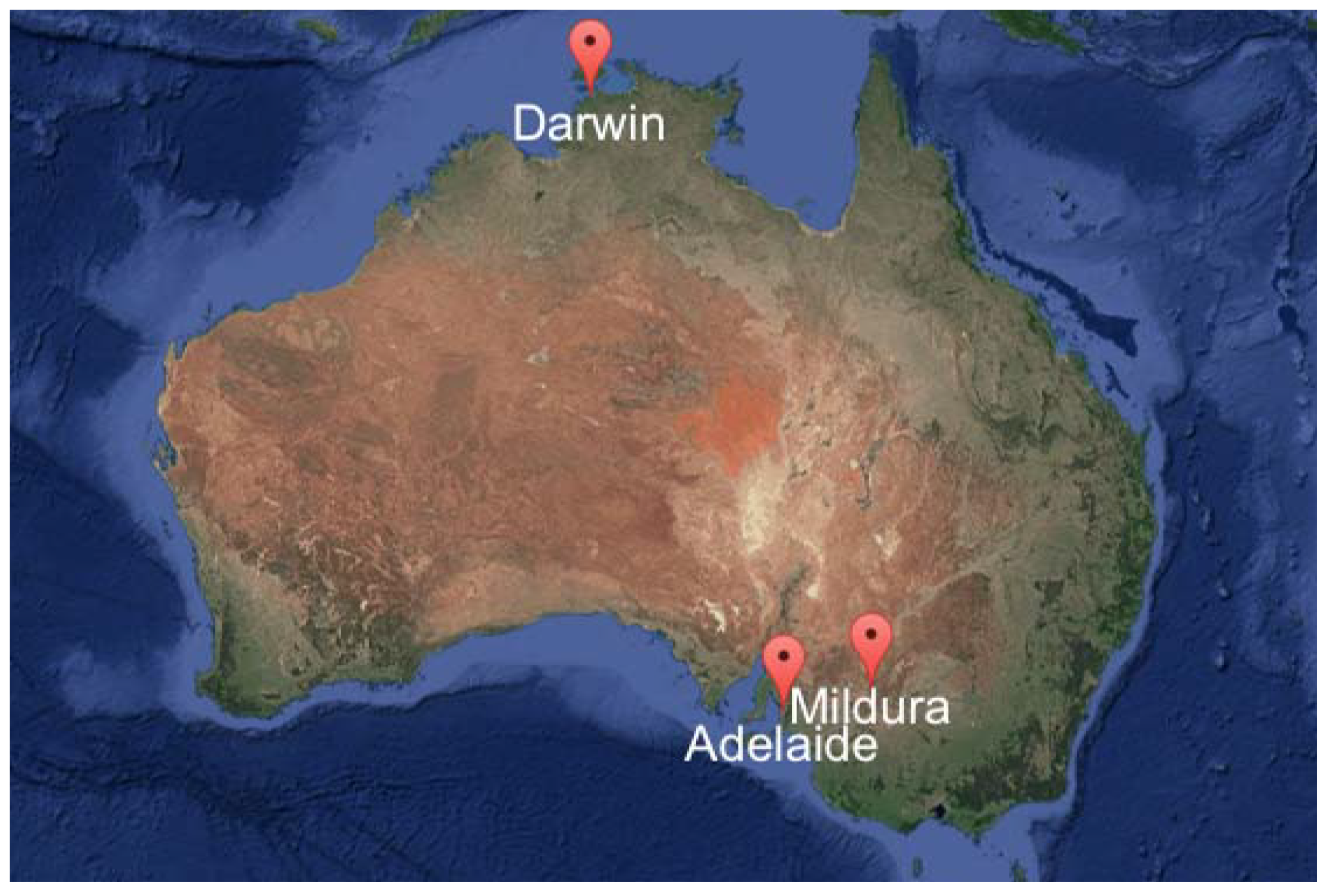
Figure 2.
GHI prediction intervals using the unconditional and conditional probabilistic forecasting methods for Adelaide.
Figure 2.
GHI prediction intervals using the unconditional and conditional probabilistic forecasting methods for Adelaide.
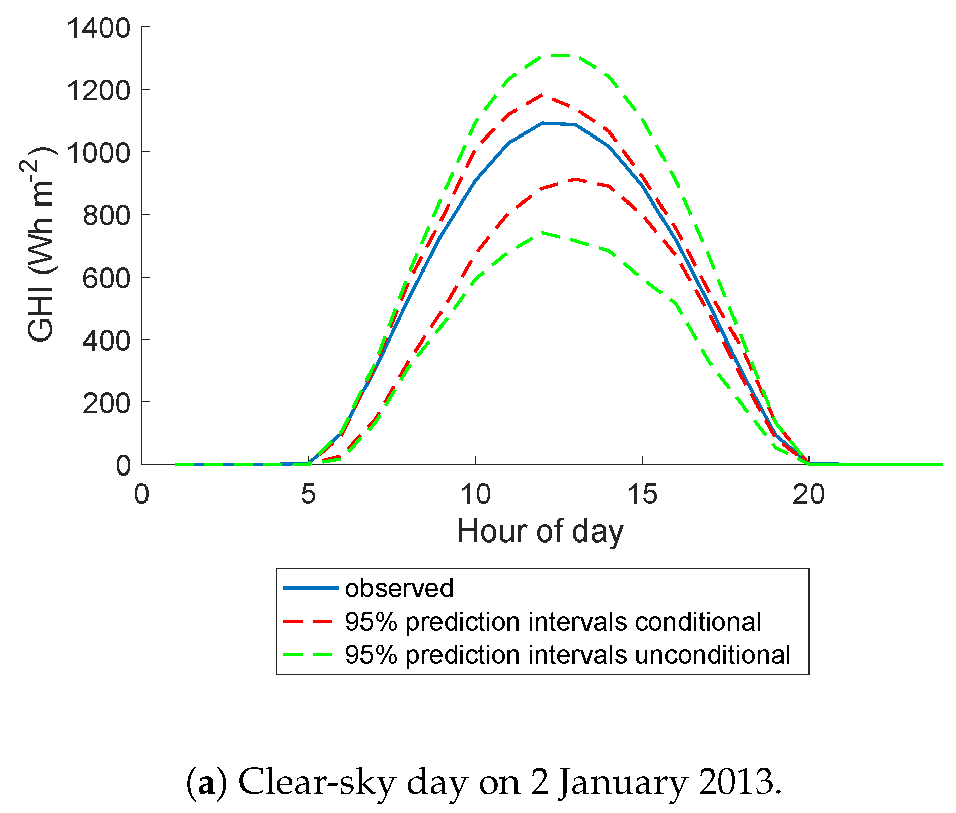
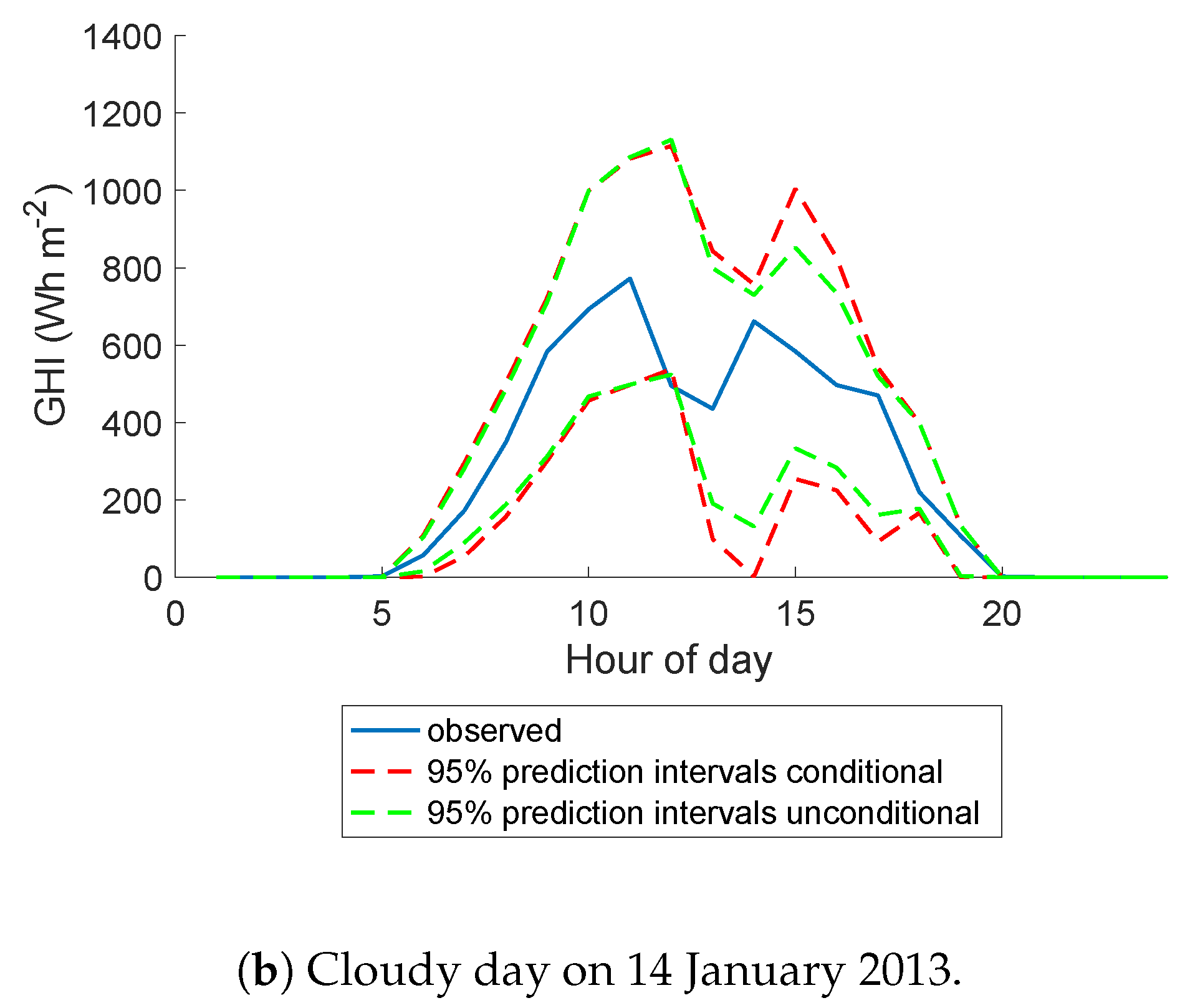
Figure 3.
GHI prediction intervals using the unconditional and conditional probabilistic forecasting methods for Darwin.
Figure 3.
GHI prediction intervals using the unconditional and conditional probabilistic forecasting methods for Darwin.
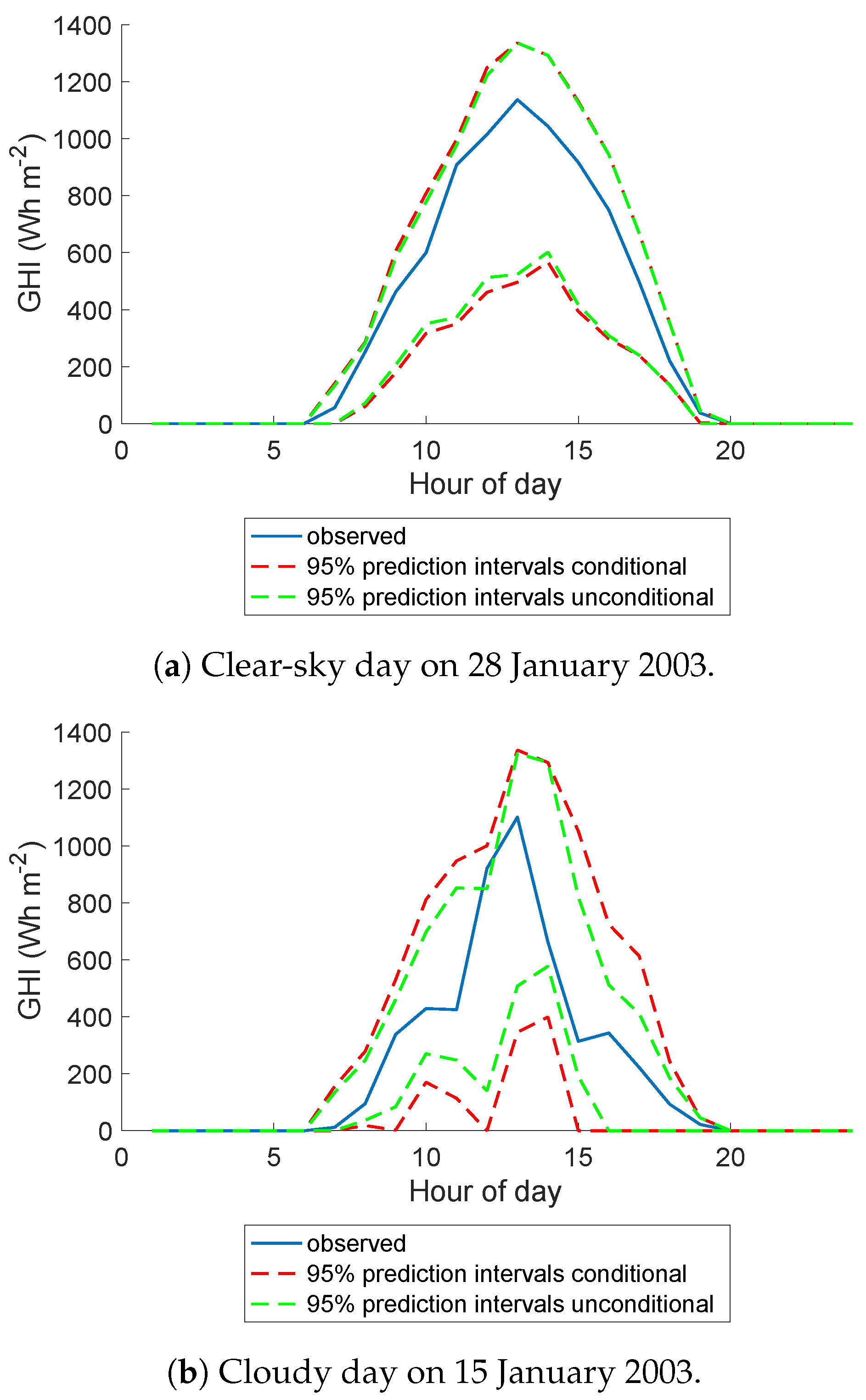
Figure 4.
GHI prediction intervals using the unconditional and conditional probabilistic forecasting methods for Mildura.
Figure 4.
GHI prediction intervals using the unconditional and conditional probabilistic forecasting methods for Mildura.
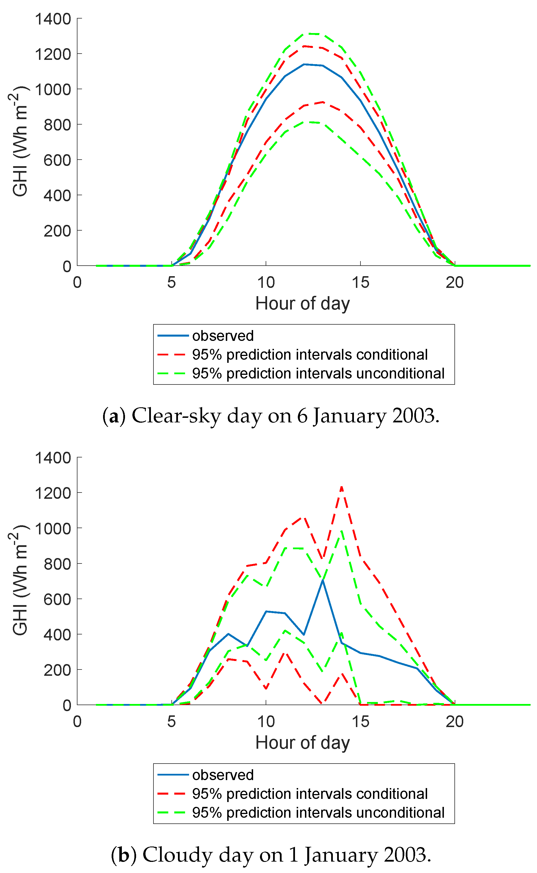
Figure 5.
Reliability of prediction intervals in the form of quantile–quantile plots over the out-of-sample period with 95% consistency bars using the unconditional and conditional probabilistic forecasting methods, for Adelaide, Darwin, and Mildura. The black line represents is the 45-degree reference line.
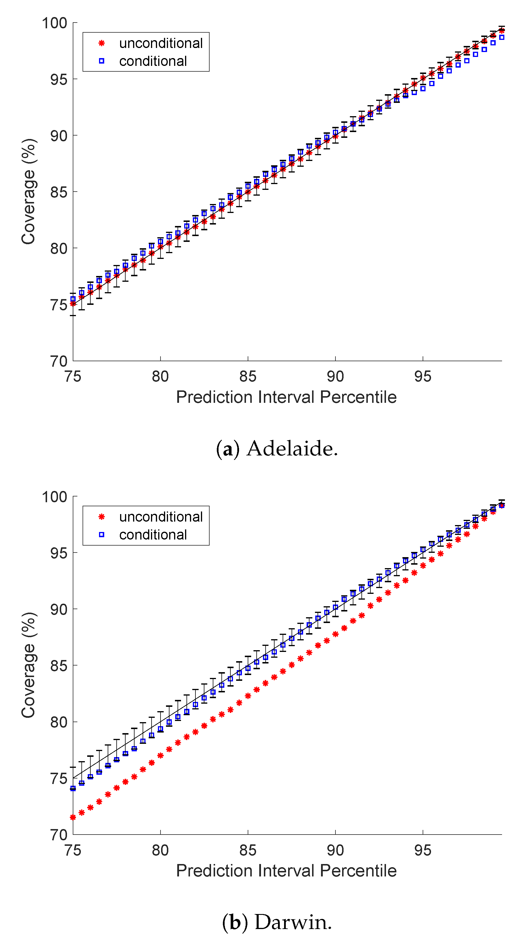
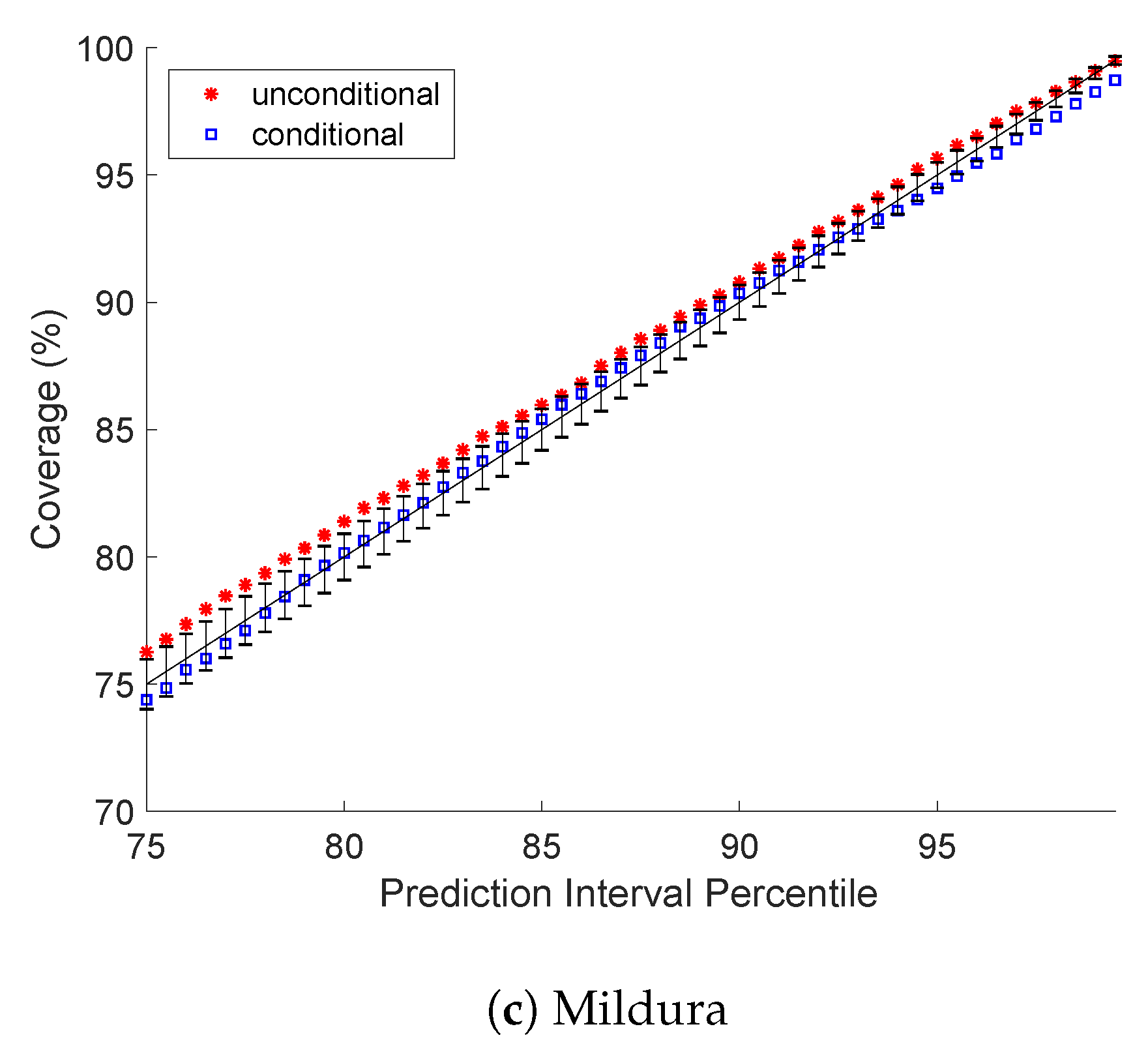
Figure 6.
Prediction interval normalized averaged width (PINAW) over the out-of-sample period using the unconditional and conditional probabilistic forecasting methods, for Adelaide, Darwin and Mildura.
Figure 6.
Prediction interval normalized averaged width (PINAW) over the out-of-sample period using the unconditional and conditional probabilistic forecasting methods, for Adelaide, Darwin and Mildura.

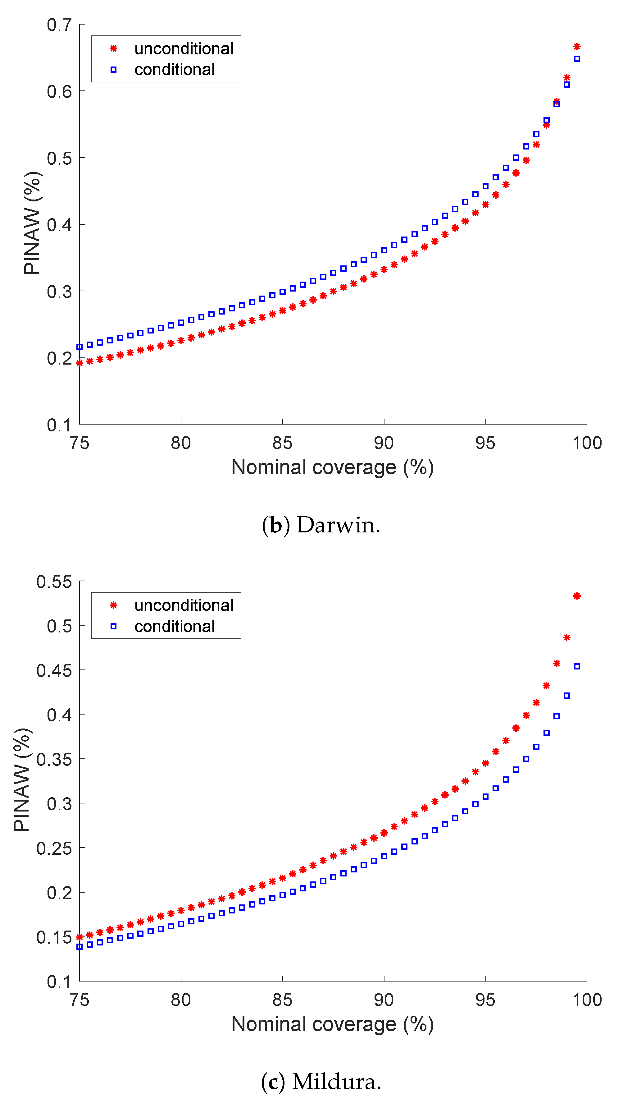
Figure 7.
Normalized Winkler score over the out-of-sample period using the unconditional and conditional probabilistic forecasting methods, for Adelaide, Darwin, and Mildura.
Figure 7.
Normalized Winkler score over the out-of-sample period using the unconditional and conditional probabilistic forecasting methods, for Adelaide, Darwin, and Mildura.
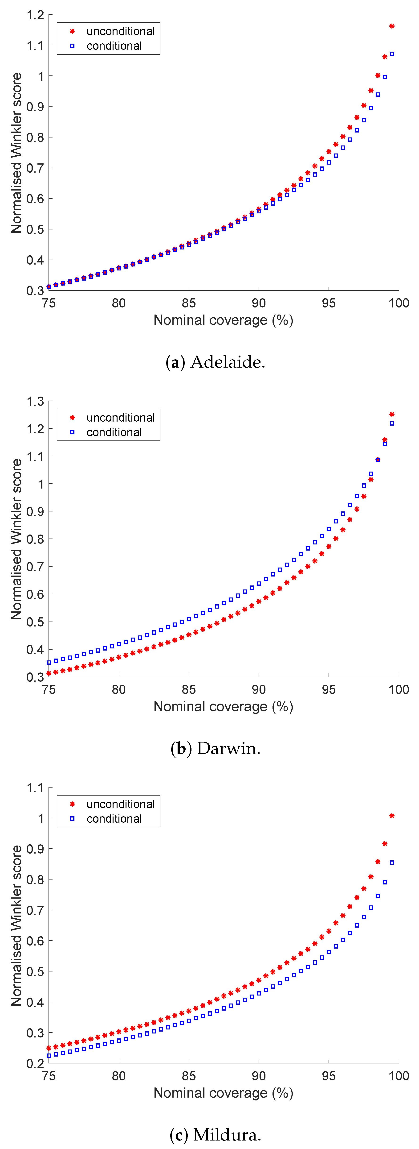
Figure 8.
Daily clearness index for one year for Adelaide.
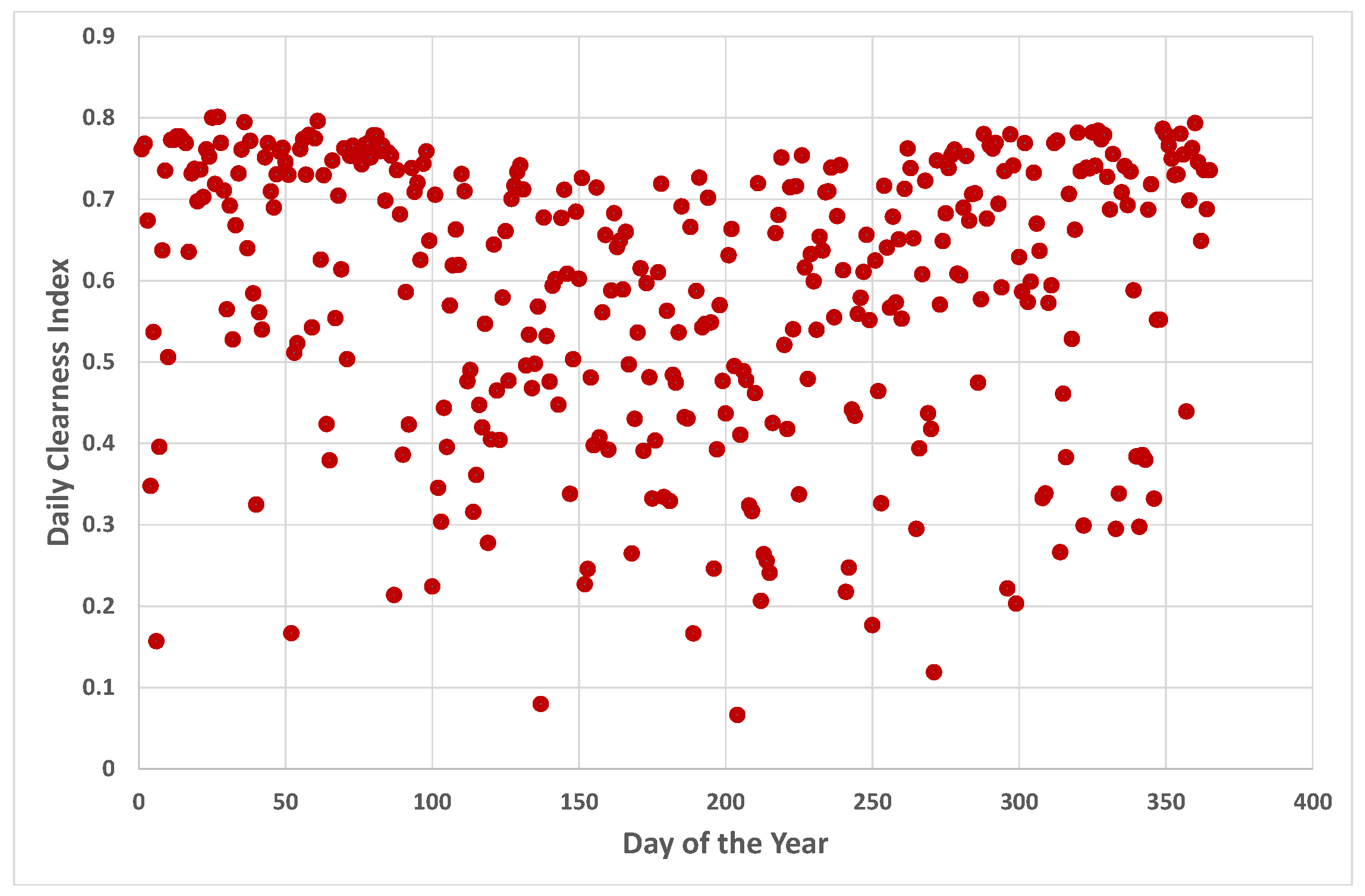
Figure 9.
Daily clearness index for one year for Darwin.

Figure 10.
Reliability of prediction intervals in the form of quantile–quantile plots over the out-of-sample period with 95% consistency bars for the unconditional and conditional probabilistic forecasting methods, for Darwin, for summer and winter seasons. The black line represents is the 45-degree reference line.
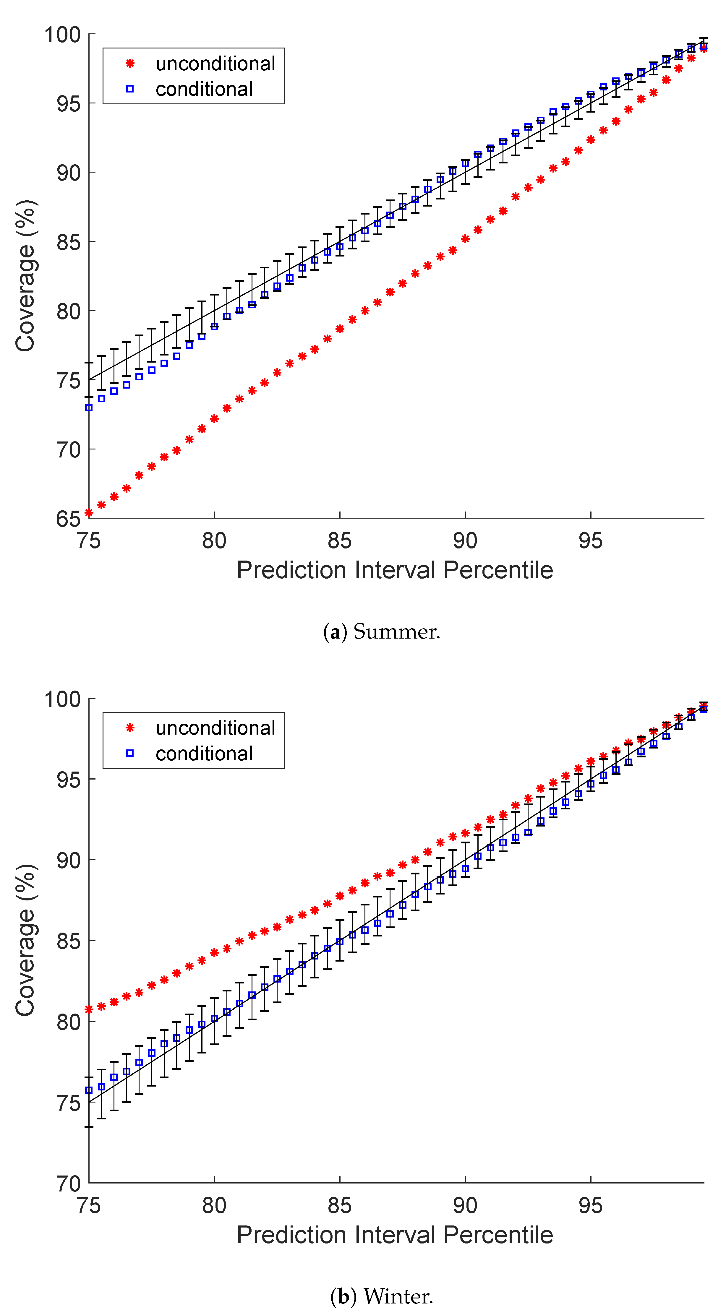
Figure 11.
Normalized Winkler score over the out-of-sample period for unconditional and conditional probabilistic forecasting methods for Darwin, for summer and winter seasons. The black line represents is the 45-degree reference line.
Figure 11.
Normalized Winkler score over the out-of-sample period for unconditional and conditional probabilistic forecasting methods for Darwin, for summer and winter seasons. The black line represents is the 45-degree reference line.

Table 1.
Data period and climate classification for the three locations.
| Location | Data Period | Köppen-Geiger |
|---|---|---|
| Climate Classification | ||
| Adelaide | 2005 to 2014 | Hot Mediterranean |
| Darwin | 1995 to 2004 | Tropical |
| Mildura | 1995 to 2004 | Semi-arid |
Table 2.
Out-of-sample normalized root means square error (NRMSE), mean bias error (MBE) and mean absolute error (MAE) for the point forecasting method for Adelaide, Darwin, and Mildura.
Table 2.
Out-of-sample normalized root means square error (NRMSE), mean bias error (MBE) and mean absolute error (MAE) for the point forecasting method for Adelaide, Darwin, and Mildura.
| Point Forecast | NRMSE (%) | MBE (%) | MAE (%) |
|---|---|---|---|
| Adelaide | 19.14 | 0.72 | 13.25 |
| Darwin | 22.74 | 0.81 | 15.83 |
| Mildura | 15.29 | 1.32 | 10.83 |
© 2018 by the authors. Licensee MDPI, Basel, Switzerland. This article is an open access article distributed under the terms and conditions of the Creative Commons Attribution (CC BY) license (http://creativecommons.org/licenses/by/4.0/).
Share and Cite
MDPI and ACS Style
Boland, J.; Grantham, A. Nonparametric Conditional Heteroscedastic Hourly Probabilistic Forecasting of Solar Radiation. J 2018, 1, 174-191. https://doi.org/10.3390/j1010016
AMA Style
Boland J, Grantham A. Nonparametric Conditional Heteroscedastic Hourly Probabilistic Forecasting of Solar Radiation. J. 2018; 1(1):174-191. https://doi.org/10.3390/j1010016
Chicago/Turabian StyleBoland, John, and Adrian Grantham. 2018. "Nonparametric Conditional Heteroscedastic Hourly Probabilistic Forecasting of Solar Radiation" J 1, no. 1: 174-191. https://doi.org/10.3390/j1010016