Abstract
Global shipping is an essential, energy-efficient enabler of trade, yet it remains a hard-to-abate sector. With shipping demand projected to continue to rise in the coming decades, identifying scalable and sustainable fuel alternatives is critical. Biofuels, and particularly biomethanol, offer a promising option due to their compatibility with existing infrastructure. However, their sustainability critically hinges on land use impacts. From this Perspective, we argue that biomethanol derived from a dedicated crop could contribute to maritime decarbonisation, with ~71–77% well-to-wake greenhouse gases (GHG) reductions under cropland-only constraints. We further point to the fact that a wider adoption faces challenges such as higher costs, limited availability, and lower energy density relative to fossil fuels. Continued research and monitoring are essential to ensure that biofuel production does not inadvertently contribute to deforestation or biodiversity loss. We underscore the need for spatially sensitive biofuel deployment strategies that align maritime decarbonisation with land-system sustainability and climate objectives.
1. Introduction
To comply with the Paris Agreement targets, decarbonisation across sectors needs to accelerate and is amongst the most urgent challenges of today. Maritime transport exemplifies an important sector, moving over 80% of the world’s goods by volume while relying heavily on fossil fuels [1]. Despite being one of the most energy-efficient modes of freight transport, the sector is a substantial source of greenhouse gas (GHG) emissions. In 2018 alone, international shipping emitted about 1.1 billion tonnes of CO2-equivalent, representing approximately 3% of global anthropogenic emissions [2]. Shipping has been responsible for around 13% of SOx and 15% of NOx emissions globally, with significant health implications near ports; however, strengthened limits on fuel sulphur and engine NOx are driving these totals downward [3,4].
As global trade continues to expand, maritime transport demand is projected to grow substantially, placing upward pressure on emissions despite ongoing gains in ship efficiency and design [1]. Projections indicate that, under business-as-usual scenarios, GHG emissions from international shipping could rise by 90% to 130% of 2008 levels by 2050 [3], jeopardizing international climate goals and highlighting the inadequacy of incremental efficiency improvements alone. This trajectory is inconsistent with pathways that meet the Paris Agreement and near-term action matters [5,6]. Since merchant ships and port infrastructure have long life spans, delaying fuel switching raises cumulative emissions and narrows future options [7]. In parallel, recent reductions in marine fuel sulphur have lowered cooling aerosols and bright ship-track clouds, which yields a small warming effect [8,9]. This strengthens the case for well-to-wake greenhouse gas reductions in this decade, while preserving the clear air quality benefits of sulphur caps.
Recognizing the challenge, regulatory bodies, notably the International Maritime Organization (IMO), have implemented mitigation measures, including the 2020 global sulphur cap and well-to-wake net-zero GHG target by or around 2050. These regulatory targets provide an essential framework but are unlikely to be met through operational and design efficiencies alone. Deep decarbonisation will require more transformative measures, particularly around alternative low- and zero-carbon fuels. Among these decarbonisation options, biofuels may seem appealing for their near drop-in compatibility with existing infrastructure and production from renewable feedstock.
Global bioenergy production accounted for approximately 12.1% of worldwide final energy consumption in 2021 (~45.9 EJ) [10]. Integrated assessment models (IAMs) project bioenergy could supply as much as ~214–245 EJ yr−1 by 2050 under stringent mitigation complying with 2 °C, substantially above today’s ~46 EJ of bioenergy [11,12]. Bioenergy has been proposed as an option for the hard-to-abate sectors, which could indicate an increase in competition for the end use of any available bioenergy on the market from, e.g., heavy-duty vehicles, aviation, as well as shipping [13]. Total liquid biofuels production is just less than one-tenth of total bioenergy production [10]. A small share of the liquid biofuels is currently consumed by ships—around 0.7 Mtoe in 2023, which amounted to less than one percent of the global liquid biofuel supply [14,15]. Most of current biofuel production goes to road transport, but as that sector adopts electrification, its long-term reliance on biofuels is expected to decline [16,17]. In contrast, chemicals, aviation, and maritime transport lack scalable, direct electrification options and are projected to become the primary users of advanced biofuels over time [18,19,20].
Among candidate bioenergy crops, sugarcane stands out for its high productivity as a C4 grass under favourable conditions. Reported yields already place it above other perennials such as miscanthus or switchgrass [21,22,23]. Trials under optimized conditions have recorded dry matter (DM) yields of ~50–84 Mg ha−1 and energy outputs of 530–870 GJ ha−1. Theoretically, fresh yields above 380 t ha−1 yr−1 (~177 t DM ha−1 yr−1) have been discussed in breeding analysis [21,24,25,26]. These benchmarks underline sugarcane’s advantage as a bioenergy crop, supporting the work of this Perspective as an exploration of the potential sustainable biomethanol supply.
Despite their promise, biofuels have been raising concerns related to land use changes, biodiversity loss, contributions to water scarcity, and competition with food production [27,28,29,30,31,32,33]. Meaningful mitigation from biofuels depends on stringent sustainability criteria, notably sourcing feedstocks that do not trigger deforestation or displacement effects (indirect land use change, iLUC) [30,34,35].
Considering these challenges and opportunities, this Perspective explores a biofuel pathway tailored to the maritime sector’s energy demand through the novel integrations of Earth system LUC dynamics paired with ship emission modelling and the life cycle assessment (LCA) literature. We use this to illustrate that such a biofuel pathway could contribute towards the decarbonisation of shipping without compromising land use sustainability.
2. The Role of Alternative Fuels in Maritime Decarbonisation
As conventional fuels like residual fuel oils (e.g., heavy fuel oil, HFO) and distillate fuel oils (e.g., marine gas oil, MGO; marine diesel oil, MDO) come under tighter emissions regulation, various low-carbon and zero-carbon options are emerging. MGO is a light distillate fuel similar to road diesel but with higher sulphur permitted, and MDO is a blend of distillates with a heavy fuel oil fraction commonly used in medium-speed and auxiliary engines [36]. Biofuels (e.g., biodiesel, biomethanol, and bio-LNG (liquefied natural gas)), methanol, liquefied natural gas (LNG), hydrogen, and ammonia are among the leading candidates as alternative marine fuels each carrying distinct advantages and technical challenges [6,35,37,38,39]. Combinations of new fuels and emissions control technologies will likely be necessary to achieve near-zero emissions in shipping [36].
Unless stated otherwise in this Perspective, all emissions are reported on a well-to-wake (WTW) basis, which includes both well-to-tank (WTT) upstream stages (feedstock production, processing, transport, and fuel synthesis) and tank-to-wake (TTW) engine exhaust during ship operation. This distinction matters for comparing fuels, e.g., LNG can show lower TTW CO2 emissions, yet lose that benefit on a WTW basis due to methane slip and upstream leakage; e-fuels (e.g., e-methanol, hydrogen, and ammonia) depend strongly on the carbon intensity of the electricity used in WTT synthesis; and biofuels must include land use change and agricultural emissions within WTT, with biogenic TTW CO2 treated according to lifecycle accounting conventions. Hydrogen and ammonia can both potentially deliver carbon-free propulsion but demand specialized handling. Hydrogen requires cryogenic or high-pressure storage, which necessitates advanced insulation and safety systems to prevent boil-off and ignition risk. Ammonia, while easier to store at ambient pressure, raises serious safety concerns for being corrosive and toxic. Additionally, ammonia combustion generates substantial amounts of NOx and N2O, necessitating advanced emissions controls [40]. LNG reduces TTW CO2 by 20–25% compared to HFO, yet methane slip undermines its climate benefits [3]. Methanol is liquid at ambient temperature and pressure and can be produced from biomass (biomethanol) or captured CO2 and renewable electricity (e-methanol). It emits minimal sulphur oxides, lower NOx, and fewer particulates, though formaldehydes can increase, but this is manageable with modern after-treatment [41,42,43].
Biofuels can often be used as drop-in fuels that can be blended in limited proportions with existing petroleum-based ones without modification [14,37]. A fundamental concern in the literature has been that the land requirements for large-scale biofuel production could jeopardize the viability of biofuels as a sustainable alternative for shipping [11,14,19]. Our Perspective challenges this notion by positing that, through sensible feedstock selection and innovative land management strategies, the production of biofuels, particularly sugarcane-based biomethanol for shipping, in this case, can be environmentally sustainable. By focusing on the utilization of existing croplands and assumptions of dietary shifts and advances in agricultural practices, it is possible to mitigate direct competition with food production and biodiversity conservation, thereby preserving critical ecosystems. This approach not only addresses the land use dilemma but also reinforces the potential for biofuels to play a pivotal role in decarbonising the shipping industry without undermining broader sustainability objectives. This position is consistent with recent optimization studies demonstrating that purposeful land reallocation can raise food supply while increasing terrestrial carbon stocks and lowering biodiversity risk, provided safeguards on forests and freshwater are enforced. This underscores that land use change, when guided by robust constraints, can free land for additional uses such as bioenergy without undermining food security or ecosystem integrity [44].
Methanol as a Marine Fuel
Methanol as shipping fuel seems promising given its practical balance of low emissions, safety, and relatively straightforward adoption., e.g., in contrast to LNG, methanol-fuelled ships would not experience methane slip issues [35,42]. Furthermore, compared to ammonia and hydrogen, methanol is significantly less toxic, does not require cryogenic containment, and can be stored in existing tanks with minimal modifications [37,39,43]. These features facilitate bunkering operations and reduce the costs and complexity of ship retrofitting [14,19,45]. Nonetheless, methanol is not directly compatible with conventional infrastructure, as it is highly corrosive and has a low flash point [37,46,47].
The production flexibility of methanol can make the transition toward cleaner production more straightforward, considering it can be produced from natural gas, coal, or biomass. Methanol from natural gas or coal is fossil-derived and yields little or no GHG benefits unless paired with carbon capture and storage. However, its existing infrastructure provides a foundation for scaling renewable pathways. Methanol derived from renewable electricity (e-methanol) or sustainably sourced biomass (biomethanol) delivers substantial emission reductions and improves local air quality. Lifecycle performance still strongly depends on the feedstock and energy used. When sourced from renewables, methanol can achieve carbon neutrality and produces fewer local pollutants than conventional fuels, thereby significantly reducing SOx, NOx, and particulate matter [31,35,42,43,48].
Recent techno-economic assessments indicate that sustainably sourced biomethanol can abate CO2 at roughly EUR 100–150 t−1 CO2-eq, typically below the cost range of onboard carbon capture options for deep-sea vessels [35]. At carbon prices in this band, the carbon value applied to a typical well-to-wake intensity gap (≈60–80 kg CO2-eq GJ−1) corresponds to ~EUR 6–12 GJ−1, closing much of today’s delivery-cost gap. Any residual difference can be bridged with contracts-for-difference or targeted operating credits designed to stabilize early investment returns (see Appendix B and Table A4 for the expanded Contract for Differences (CfD) analysis). Present day production costs of biomethanol vary depending on feedstock price and plant scale/efficiency, and co-product credits are expected to reduce by 2050 through learning and scale effects [43]. Port-paired siting and modular plants co-located with sugar mills can further reduce logistics costs and improve traceability, provided strict sustainability safeguards (no-deforestation feedstocks, verified LUC) are maintained. Distribution logistics remain a decisive factor in biomethanol competitiveness and strongly influence fuel uptake. Hence, locating production near major ports minimizes inland haulage, enables direct integration into tanker networks, and reduces well-to-tank emissions [38,49,50].
In comparison to other options, biomethanol offers a practical compromise between technical readiness and decarbonisation potential. Key advantages and disadvantages of biomethanol as a marine fuel are summarized in Table A1. Hydrogen and ammonia may achieve deeper long-term reductions (often exceeding 85% GHG savings on a WTW basis), but their adoption requires extensive vessel redesign, port infrastructure, and safety systems [42,45]. LNG is more mature and widely available, but its lifecycle benefits remain modest or even negative without strict methane controls [3,51].
Against this backdrop, biomethanol combines near-term feasibility, adaptability to modified engines and bunkering systems, and substantial lifecycle GHG reductions (~70–80% when land use impacts are safeguarded), positioning it as one of the most competitive and pragmatic near-term alternatives for maritime decarbonisation [35,39,43].
3. Integration of Land Use Modelling, Shipping Emission Modelling, and Lifecycle Assessment
This Perspective examines the prevailing assumption that large-scale deployment of biofuels for shipping is constrained by unsustainable land competition. We explore this by demonstrating a case where sugarcane-derived biomethanol is used as a substitute for conventional marine fossil fuels and evaluate both the fuel switching emissions impacts and the Earth system feedback from associated land use dynamics.
To this end, we integrated land use modelling using the Norwegian Earth System Model (NorESM2) [52] and global maritime energy demand projections from the MariTeam model [53]. NorESM2, with its land component, the Community Land Model Version 5 (CLM5) [54], is a fully coupled climate–carbon cycle model capable of reflecting biogeophysical and biogeochemical responses to land use changes over time and space. The model simulates land–atmosphere feedback that can influence local temperature and precipitation. This feedback is included in our simulation cases, which reflect biogeophysical as well as biogeochemical responses to cropland reallocation. We use CLM5 in NorESM with prognostic soil carbon–nitrogen cycling. Nitrification and denitrification produce soil N2O as functions of soil mineral nitrogen, temperature, and moisture. Ammonia volatilization and crop nitrogen uptake costs are represented. Agricultural management is simulated through the global crop module with time-varying irrigation and fertilization. Consequently, agricultural emissions emerge from process representation, rather than fixed emission factors [54,55].
We evaluate model output as spatially aggregated decadal means rather than site-specific temporal trajectories, averaging over a long period and long after model simulation starts, smoothing strong early carbon dynamics that typically occur after land conversion that have been documented across empirical syntheses and field studies, including sugarcane payback assessments [56,57,58,59].
Using detailed inputs on ship type, speed, and routing, the bottom-up MariTeam model quantifies global fleet emissions. We apply it to derive current energy demand, current emissions, and comparative emissions for methanol use. Historic data from the literature indicate that shipping’s energy demand has ranged between about 8 and 15 EJ [3,60,61,62] in the last 10 years, depending on whether the scope is global or limited to international shipping, and on whether estimates are derived using top-down or bottom-up approaches. In the MariTeam model, the global shipping energy demand is around 14 EJ yr−1 for the period of 2018–2021, with a projected increase to 14–20 EJ yr−1 toward the mid-century [63]. Figure 1 illustrates the geographical distribution of shipping energy use, alongside its regional aggregation according to the MESSAGEix R11 regions [64]. The results reveal distinct energy use hotspots along major trade corridors. These spatial patterns highlight where decarbonisation efforts and infrastructure for alternative marine fuels should be prioritized, and help targeted deployment strategies. Building on this, we show candidate sugarcane cultivation areas that could supply biomethanol production in major demand regions (see Figure 2).
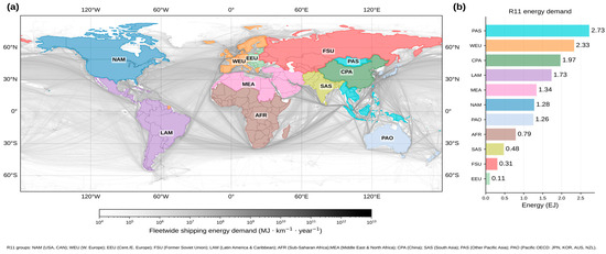
Figure 1.
(a) Geographical distribution of annual average energy consumption (MJ km−2 yr−1) from global shipping from the MariTeam model for 88,000 ships, including merchant and working vessels engaged in domestic and international voyages, based on shipping activity from 2018 to 2021. Darker tracks correspond to higher density of traffic and greater energy demand along major corridors. (b) Annual energy use per 11 regions, as defined by MESSAGEix [64], where energy use is allocated to port of departure per voyage. Bars indicate the aggregated annual shipping energy demand attributable to each region. The MariTeam model shows a total global maritime energy demand of 14 EJ yr−1.
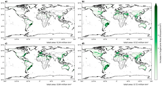
Figure 2.
Candidate sugarcane cultivation areas (thousand km2) in regions with high maritime energy demand. Left panels (a,c) consider coastal-adjacent allocation areas, applying a ≤~400 km shoreline mask to prioritize port-proximate siting; right panels (b,d) depict the regions with high maritime energy demand not limited to coast adjacency.
To estimate the impact of this land use pathway, we link the land use scenario to maritime energy demand and emissions. We simulate a dedicated bioenergy crop scenario in which sugarcane expansion occurs within existing cropland boundaries, thereby avoiding direct deforestation or expansion into natural ecosystems. Sugarcane area was introduced by reallocating land within the existing cropland category in the Shared Socioeconomic Pathway 5-3.4 (SSP5-3.4) scenario, as defined by the Land Use Harmonization version 2 (LUH2) land use inputs to the land component of NorESM2 [52,65,66].
Land availability within the existing cropland area covers a range from 0.24 to 0.84 million km2 in our illustrative cases (Figure 2). Not only does the total area matter but also the location. Expansion is mostly in coastal regions (the two nearest inland grid cells in NorESM-LM) and constrained to MESSAGEix R11 regions with high maritime energy demand (more than 1 EJ yr−1). To test geographically targeted deployment, two scenarios apply an explicit coastal constraint: candidate production sites are restricted to locations within ~400 km of the coast and proximate to major bunkering hubs. This coastal siting prioritizes short overland haulage, minimizes upstream emissions and costs (≤~1–2 g CO2-eq MJ−1 and ≤~EUR 1 GJ−1), and limits additional infrastructure needs for moving feedstock or fuel over long distances. To bound the effect of inland transport, we convert distance-based freight emissions to g CO2-eq MJ−1 using typical emission factors (EF) and methanol lower heating value (LHV) (19.9 GJ t−1). See Appendix B for more discussion on upstream logistics of coastal siting.
Using the NorESM simulation output, we calculate the potential annual production of biomethanol from the added sugarcane yields in selected regions (conversion chain in Appendix B). Regions selected are pre-screened to exclude biodiversity hotspots and protected areas. Based on the above-ground net primary production (AGNPP) of the dedicated bioenergy crop and biomass-to-methanol conversion factors (as explained in Appendix A.2), the annual biomethanol is estimated per simulation year for each case [46,67]. Cultivation areas corresponding to biomethanol energy yields of about 14, 16, 19, and 20 EJ yr−1 are illustrated in Figure 2.
Supplying 14–20 EJ yr−1 would require less than 6% of the current cropland and less than 5% of the projected global cropland area in 2050 in our illustrative scenarios. Reallocating cropland area for bioenergy crop cultivation is typically assessed under assumptions of technological advances, dietary changes, and reductions in food waste. Such shifts can suitably free agricultural land by improving production efficiency and loss management [68,69,70,71]. To underpin this, we embed our scenario in complementary studies on the supply side intensification and on the demand-side land sparing.
Sathyanadh et al. model the increase in sugarcane area, as a C4-photosynthetic pathway crop for bioenergy; the potential is up to 5.2 million km2 by 2100 [66]. Here, we limited this potential area expansion to the land needed to satisfy projected shipping energy demand by Kramel et al. [63] and only within targeted regions of existing cropland, excluding forests, savannas, wetlands, and other natural ecosystems. Such conservative framing aligns with boundary-informed land use optimization studies that show agricultural expansion is compatible with higher food supply and environmental gains if confined to suitable cropland and coupled with pasture contraction, yield improvements, and water safeguards [44,70].
The feasibility of this land reallocation is supported by two general complementary strands of evidence. On the supply side, global modelling indicates that yield gap closure and spatial optimization could reduce the cropland needed to maintain current production by approximately 50% [72]. In parallel, increasing cropping intensity and reallocating crops could raise biomass production by approximately 148% without expanding cropland [73], while multiple cropping could expand harvested area by 7–35% in suitable regions (enhancing production without increasing physical cropland extent) [74]. These results indicate a substantial land buffer embedded within current agricultural systems.
On the demand side, waste reduction and dietary changes further reduce the land required for food production. Roughly 23% of global cropland currently supports food that is never consumed; halving these losses could free 9% of agricultural land [68,75]. Dietary shifts could reduce the land needed for food production by 16–55% globally, depending on the extent and type of change [68]. These measures also reduce GHG emissions and improve resource efficiency [71,76].
The combined land-sparing potential of these strategies exceeds the cropland reallocation (approximately 5%) assumed in our LUC cases, providing a credible land buffer for sustainable bioenergy crop deployment without disregarding food production or natural ecosystems. We acknowledge three main sources of uncertainty. First, the adoption of dietary change and food waste reduction depends on socio-economic and policy contexts, which vary widely by regions. Second, yield gap closure, cropping intensification, and spatial reallocation are constrained by agronomic, infrastructural, and environmental conditions that may limit their implementation potential. Third, interactions among these interventions may generate trade-offs or rebound effects, such as input intensification pressures or market-mediated land expansion. Despite these uncertainties, the combined land-sparing potential remains considerably larger than the 5% cropland reallocation assumed in our illustrative cases, supporting the robustness of the argument.
To avoid displacing food production, we assume a balanced package of yield increases from improved management practices, moderate diet shifts away from the most land-intensive calories (e.g., ruminant meat), and food-loss/waste reductions. Reallocating cropland to bioenergy is feasible only under safeguards that protect nutrition, biodiversity, and water. Recent studies find that halving food loss and moderating consumption of land-intensive animal products can increase available calories by more than one third, expanding the feasible space for additional land-based uses [70,75,77]. Our diet assumptions are illustrative not prescriptive: they represent one practical path to free land without converting natural ecosystems, following previous studies like Muri (2018) [78] and Sathyanadh et al. (under review) [66].
We compared lifecycle (well-to-wake) GHG emissions of sugarcane-based biomethanol with those of marine fossil fuels (heavy fuel oil and marine gas oil) using the representative literature emission factors [3,39,42,45,51]. The biomethanol inventory includes tank-to-wake combustion and land use related emissions from NorESM (i.e., changes in soil and vegetation carbon stocks).
The mean interannual changes in combined soil and vegetation carbon stocks shows that reallocating existing cropland to sugarcane results in a terrestrial carbon source ranging from 0.04 to 0.08 GtC yr−1. Biogenic CO2 is re-emitted at combustion and re-assimilated over the cropping cycle; net WTW results hinge on LUC carbon stock changes and time profiles. Whereas in the case of marine fossil fuels, upstream (well-to-tank) CO2-eq emissions account for an additional 15–25% beyond combustion emissions [43].
Our simulations quantify direct land use change within NorESM2 CLM5; they do not endogenously represent indirect land use change (iLUC) driven by market responses when cropland is reallocated. iLUC may displace food or feed production into new locations, with knock-on effects for forests, pasture, biodiversity, and water stress. The sign and magnitude are model- and context-dependent and reflect assumptions about baselines, yields, trade, and policy [27]. Some current regulatory practices incorporate iLUC using economic model ensembles, acknowledging the need for an iLUC term while also reflecting the uncertainty in its value [79]. For transparency, we report quantitative iLUC sensitivities (+5/+10/+20 g CO2-eq MJ−1) in Appendix B. Credible mitigation requires enforceable no-deforestation criteria, traceable supply chains, and jurisdictional land use controls consistent with low-iLUC-risk approaches. Because climate change can influence yields and trade patterns and land competition, future assessments should endogenize iLUC by coupling land models with economic land use models and testing multiple climate scenarios.
The production phase of biomethanol, excluding land use change, has varying emissions depending on the feedstock and conversion pathway [43,80,81]. We consider an additional 10 g CO2-eq MJ−1 added to land use change emissions, as derived from this discussion’s simulation cases, which contribute an additional 10.5, 10.3, 15.8, and 10.4 g CO2-eq MJ−1 for the 14, 16, 19, and 20 EJ yr−1 supply cases, respectively. A Monte Carlo analysis using 10,000 draws based on these inputs indicates case medians for total biomethanol intensity spanning ~20–26 g CO2-eq MJ−1, with a 5th to 95th percentile envelope of 13.7 to 33.8 g CO2-eq MJ−1 across the cases (see Appendix B Figure A1, Table A2 and Table A3). For comparison, the lifecycle GHG emissions of conventional marine fuels such as HFO or MGO are typically in the range of 85–95 g CO2-eq MJ−1, when including both combustion and upstream emissions [42,45,51,82]. Thus, the simulations yield roughly 71–77% (no iLUC), with a 5th to 95th percentile envelope of about a 62–85%, reduction in CO2-eq emissions relative to conventional fossil fuels in a full lifecycle Perspective on an energy equivalent basis. For more details on methods and assumptions, see Appendix B.
It should be noted that these reductions are sensitive to land use change assumptions, regional yield factors, and biophysical feedback. Regions with minimal soil carbon loss and high biomass productivity could offer higher GHG savings. Longterm analyses are required to capture interannual yield variability, market-driven indirect land use changes, and process-specific emissions.
Combined modelling outputs indicate that sugarcane-based biomethanol can substantially contribute to maritime decarbonisation if cultivated on suitable croplands. As yields and LUC emissions vary by region and agricultural practices, sustainable outcomes depend on minimizing LUC emissions and ensure high yields. Integrating high-resolution spatial analysis with economic modelling will be essential for policy and investment decisions.
4. Future Directions
Decarbonising international shipping from a well-to-wake Perspective by mid-century remains urgent, with the majority of the fleet still reliant on petroleum fuels. Recent cost–benefit comparisons show that methanol, especially when synthesized sustainably, can reduce SOx and particulate matter (PM) to almost zero. When produced with near-zero-carbon inputs (e.g., e-methanol), methanol can approach ~90–95% WTW CO2 reductions, and sustainably sourced biomethanol typically achieves lower (70–80%) but still substantial reductions. TTW NOx emission reductions are typically 10s or up to 80% relative to heavy fuel oil if after-treatment is used [47], though cost parity with fossil fuels remains policy-dependent (e.g., carbon pricing, mandates) [39,83].
Sugarcane offers a high yield C feedstock that can leverage mature (e.g., Brazil) agro-industrial systems, potentially supplying maritime demand without the new conversion of natural ecosystems if constrained to existing cropland and robust safeguards. This is consistent with integrated assessments showing that reallocating cropland within planetary boundary limits is feasible if coupled with reducing food waste and higher nutrient-use efficiency diets, which together reduce the pressure on the land and biodiversity [77].
Building on the insights presented in this Perspective, we identify several key priorities: richer system-wide modelling is needed to capture cross-sectoral indirect effects on food security, local ecosystems, and climate, highlighting the need for more studies like this combining agricultural land use and climate modelling with bottom-up engineering-based shipping models rather than treating each independently. Well-to-wake system boundaries needs to be defined and applied: treatment of biogenic CO2, land use emissions, co-products, and blend accounting. Embedding environmental Monitoring, Reporting and Verification (eMRV) is needed to quantify non-GHG impacts (biodiversity, water, and air quality), as well as alignment with established certification schemes and standards (e.g., International Sustainability and Carbon Certification (ISCC), the European Union’s Renewable Energy Directive (RED and RED II) [14,20]) that require feedstock traceability and no-deforestation criteria. And, in practice, reallocating cropland would require standards and monitoring (traceable, no-deforestation feedstock; water/biodiversity “no-go” zones) and just transition measures for farmers (tenure, income, and benefit sharing).
Another key area is the need for robust techno-economic analyses that reflect spatial and operational realities. Assessments at country or port level under varying carbon pricing and subsidy regimes, combined with the exploration of modular, decentralized refineries co-located with sugar mills or ports, can address spatial and scale-dependent cost dynamics of sugarcane-derived biomethanol. Here, digital twin models can support techno-economic analysis by enabling the scenario-based assessment of learning curves, economies of scale, and policy measures. Given likely competing claims from aviation and chemicals, port-paired production bunkering corridors concentrate early volumes where traceability, certification, and enforcement are strongest, while minimizing transport losses and costs.
Recent analyses suggest sector-wide switching to biomethanol only becomes cost-effective above current Emissions Trading System (ETS) and at carbon prices of roughly EUR 100–150 t−1 CO2. Harahap et al. report thresholds above ~EUR 100 t−1 CO2; Kanchiralla et al. report abatement costs near ~EUR 100 t−1 CO2 for biomethanol; and Flodén et al. show that at EUR 90–100 t−1 CO2, switching is viable for only a small share of voyages, whereas above EUR 150 t−1 CO2, it becomes competitive across ship types. Using a well-to-wake carbon intensity (CI) gap of ~60–80 kg CO2-eq GJ−1, a carbon price of EUR 100–150 t−1 CO2 yields a carbon credit of ~EUR 6–EUR 10.5 GJ−1, leaving a residual carbon CfD requirement of ~EUR 0–EUR 3.6 GJ−1 across our cases (see Appendix B Table A4). These highlight a remaining policy gap and imply that supplementary instruments (e.g., targeted mandates, innovation funds) are required alongside the ETS and European Union (EU) FuelEU to achieve material uptake [35,84,85,86].
Recent analyses highlight the potential of CfDs as a mechanism to encourage early low-carbon investments by guaranteeing a stable carbon price and enabling bankable projects in hard-to-abate sectors [87]. Conventional CfDs protect investors only from downside risk but do not capture surplus revenues when prices rise. Hence, a two-sided, indexed CfD could deliver more efficiency and equitability in mature carbon markets [88,89]. The contract would link payments to (i) a carbon price index, (ii) biomass or feedstock cost indices, and (iii) a marine fuel benchmark. An optional price collar and staged volumes could limit budget risks [87,88,90]. Although such multi-indexed designs have yet to be applied in maritime contexts, the principle extends naturally from the power and hydrogen sectors and merits pilot implementation under close regulatory oversight [88,91,92].
Launching case studies and pilot projects is important for empirical validation, converting vessels to biomethanol, and generating real-world data on fuel performance, engine efficiency, and infrastructure needs. Investment in biomethanol infrastructure and vessel adaptation is hindered by the lack of operational data and demonstrated demand, while real-world data and demand cannot materialize without initial deployment. Upfront grants to build the first plants and convert existing ships should therefore be prioritized. A phased approach can support this process: pilots can be initiated in 2025–2030 on a few priority routes where ports and governments agree to act together. These pilots should coincide with early regulatory incentives such as the EU Emissions Trading System (EU ETS, effective 2024) and the FuelEU Maritime regulation (2025), which reward low-GHG fuels [14,86]. Given the cost thresholds above, these instruments can catalyze pilots.
Signing cooperation deals between port pairs guarantees buyers for the new fuel and provides insurance and risk-sharing so investors feel confident to build. Building on these efforts, early scaling from 2030 to 2035 can target clusters of strategic ports. Broader deployment post-2035 should be contingent on sustainability safeguards, including verified lifecycle GHG reductions, robust land use governance, and credible certification.
Such a phased, spatially targeted demonstration project could turn a “chicken or egg” dilemma in sustainable biofuel use in maritime transport into learning loops that will continue feeding data back into models, improve technology readiness, and inform evidence-based policy. Policy incentives, robust land management, and coordinated action among the industry, policymakers, and researchers are essential to overcome economic and logistical barriers, ensuring that maritime decarbonisation aligns with global sustainability goals.
5. Conclusions
This Perspective argues that sugarcane-derived biomethanol can provide a viable and climate-effective marine fuel within sustainable land use guardrails. Under illustrative cases that reallocate existing cropland (no encroachment into forests or other natural ecosystems), we estimate that the shipping sector’s projected mid-century energy demand of 14–20 EJyr−1 could technically be supplied with lifecycle GHG reductions of roughly 70–78% relative to marine fossil fuels, not accounting for iLUC. ILUC could reduce this climate benefit to ~60–66% under a +10 g CO2-eq MJ−1 iLUC penalty. These outcomes are conditioned on high-yield regions, careful water management, and minimized losses of soil and vegetation carbon. Sustainability is therefore not guaranteed; iLUC risks, biodiversity impacts, and water stress can erode climate benefits; and sustainable biomass is finite amidst rising demand from other hard-to-abate sectors. LUC dynamics are expected to dominate uncertainty, underscoring the need for high-resolution spatial siting and end-to-end eMRV.
A key advantage of biomethanol lies in the readiness for near-term adoption through its compatibility with existing engines and bunkering infrastructure. Regulatory drivers such as EU ETS and FuelEU Maritime can accelerate uptake. Yet, infrastructure investment and supportive policies are essential to bridge the cost gap with fossil fuels. We therefore recommend (i) the adoption of robust certification and land governance safeguards; (ii) port-paired pilot projects (near-term: 2025–2030) with transparent eMRV; (iii) techno-economic assessments at the port/corridor level under carbon pricing and mandate scenarios; and (iv) integration of iLUC-enabled land energy economic modelling to capture cross-sector competition.
In summary, sugarcane-derived biomethanol is not a stand-alone solution but a technically feasible, immediately deployable pathway that can provide meaningful emission reductions when combined with efficiency improvements, demand-side measures, supportive economic policies, and strong regulatory safeguards. Continued interdisciplinary research and multi-stakeholder collaboration are crucial to optimize this biofuel strategy and align maritime decarbonisation with global climate and sustainability goals.
Author Contributions
Conceptualization; methodology, H.E. and H.M.; software; formal analysis; data curation; validation, H.E., H.M. and D.K.; resources; supervision; funding acquisition, H.M.; writing—original draft preparation, H.E.; writing—review and editing, H.M. and D.K.; visualization, H.E. and D.K. All authors have read and agreed to the published version of the manuscript.
Funding
This research was funded by The Research Council of Norway projects Bio4-7Seas (grant number 302276), and CLIMMS (grant number 294771); Nord_H2ub project (Rally to the Valley: Establishing Hydrogen Value Chains for the Nordics) funded by Nordic Energy Research; European Union’s Horizon 2020 research and innovation programme under grant agreement No. 869357 (OceanNETs), and under grant agreement No. 101037428 (ENERGICA). The simulations were performed on resources provided by Sigma2—the National Infrastructure for High-Performance Computing and Data Storage in Norway under projects NN9576K, NS9576K, and NS9083K.
Data Availability Statement
The original contributions presented in this study are included in the article. Further inquiries can be directed to the corresponding author.
Conflicts of Interest
The authors declare no conflicts of interest.
Appendix A
Appendix A.1. An Overview of Biomethanol as a Marine Fuel

Table A1.
Summary of advantages and disadvantages of biomethanol as a marine fuel.
Table A1.
Summary of advantages and disadvantages of biomethanol as a marine fuel.
| Aspect | Advantages | Disadvantages | Example References |
|---|---|---|---|
| GHG emissions | Significant WTW CO2 reductions (up to 70–80%) compared to fossil marine fuels when produced from sustainable feedstocks with no iLUC. | GHG benefits sensitive to LUC and feedstock source; iLUC could offset savings. | [35,43] |
| Air pollutant emissions | No SOx, lower particulate matter, and lower NOx emissions compared to HFO; no methane slip. | Still emits CO2 on combustion; NOx control may be required (e.g., Selective Catalytic Reduction (SCR) or Exhaust Gas Recirculation (EGR)). | [42,47] |
| Water and land impacts | High-yield crops like sugarcane can produce large volumes of feedstock on relatively small land area if managed well. | Water-intensive crops may strain local resources; large-scale monocultures can reduce biodiversity and degrade soils; and can add pressure to planetary boundaries for land, water, and nutrients flows if scaled. | [28,29,93] |
| Technical compatibility | Liquid at ambient temperature and pressure; can be stored in modified existing tanks and bunkering infrastructure relatively easy to adapt; simplifies drop-in transition relative to cryogenic fuels. | Lower volumetric energy density (~50% of HFO) requiring larger tanks or more frequent refuelling; corrosive to some materials; and materials compatibility upgrades may be needed. | [37,39,45] |
| Safety | Lower toxicity and handling risks than ammonia; easier storage than cryogenic hydrogen. | Flammable with low flash point/low visibility flame; toxic if ingested; and requires strict handling protocols. | [19,43] |
| Economic factors | Potential cost reductions with scale-up and learning; co-location with existing agro-industrial systems (e.g., Brazilian sugarcane) can reduce logistics costs. | Currently more expensive than fossil fuels; production costs depend on feedstock price, plant efficiency, and policy incentives. | [19,43,45] |
| Scalability and supply | Multiple production pathways (biomass, e-methanol) allow gradual transition to low/zero-carbon feedstocks. Demand-side changes such as halving food loss and moderate diet shifts can free land for bioenergy without threatening food security. | Sustainable biomass availability is limited; competition with aviation and other sectors could constrain supply. | [11,29,70] |
Appendix A.2. Conversion Pathway Context
In this study, we model a thermochemical lignocellulosic route to methanol (oxygen-blown gasification → syngas clean-up/shift → Cu/ZnO/Al2O3 synthesis → distillation), consistent with peer-reviewed overviews of syngas-to-methanol chemistry and process integration [35,42,46,90,94]. Alternative bio-routes exist but are not quantified here—notably reforming of biogas to methanol and hydrogenation of biogenic CO2 with renewable H2 (bio-e-methanol) [95,96,97,98]. The literature indicates that performance and costs depend strongly on feedstock quality, gas clean-up severity, recycling, and utility integration, and techno-economic analyses (TEAs) report a wide range with feedstock and capital expenditure (CAPEX) as primary drivers [43,46,80,90,99,100]. Our land use-led analysis therefore holds the pathway constant (lignocellulosic gasification) and treats production parameters within literature-consistent ranges.
Appendix B
Appendix B.1. Biomethanol Production from AGNPP
We impose a coastal siting constraint, restricting candidate areas to within ~400 km of the shoreline and proximate to major bunkering hubs. The radius approximates a one-day rail/road haul, reducing upstream logistics emissions, simplifying traceability and (e) MRV, and lowering new infrastructure needs for moving feedstock or fuel long distances. Because experiments were run on the NorESM-LM native grid, we implemented the coastal proximity constraint by selecting the two inland grid cells adjacent to the coastline. As grid-cell size varies with latitude, the effective coastal distance is not uniform across regions. A simple robustness test comparing effective radii of ~250 km and ~400 km yields similar qualitative outcomes (supply potential and hotspot locations), indicating that our main conclusions are insensitive to the precise radius choice. The distance between biomass supply sources and the port matters primarily because it influences logistical costs and emission leakage. Restricting supply partially affects the final cost and emissions as other factors (e.g., mode of transport and its energy source, quantity of the commodity, loading/unloading costs, and regional policies and limits) are also at play [101,102,103]. Coastal siting (≤~400 km to major bunkering hubs) minimizes upstream emissions and costs and strengthens chain-of-custody and eMRV, while the 250–400 km choice has negligible effect on central WTW results.
The potential energy yield of biomethanol was derived by linking modelled aboveground net primary production (AGNPP) to harvestable biomass, methanol mass, and methanol energy. AGNPP as a carbon flux [g C m−2 s−1] aggregated over the study region and averaged across 10 simulation years in each case to derive annual totals. To translate carbon fluxes into dry matter biomass, we adopted the Intergovernmental Panel on Climate Change (IPCC) guidelines’ default carbon fraction of 0.5 in dry biomass [104]. We assumed that 80–85% of AGNPP is harvestable biomass based on the recent literature [105]. Dry biomass was then converted to methanol using yields from gasification production pathways, which range ~0.3–0.65 kg MeOH per kg dry biomass, depending on feedstock and process configuration [43,46,106]. For our central estimate, we adopted the median value. Methanol output was then expressed as energy using the lower heating value, 19.9 GJ t−1, to obtain annual biomethanol energy potential (EJ yr−1):
where Y is number of case’s simulation years (here 10), S second per year, fc carbon fraction of dry biomass, h harvestable share of biomass, yieldMeOH conversion yield of dry biomass to methanol via gasification, LHVMeOH energy per mass of methanol, and the factor 10−15 collects unit conversions g to tonnes and GJ to EJ.
Regional differences in biomass production are represented through the prognostic NorESM-CLM5 simulations, which capture spatial variability in climate, soils, and land use under the chosen SSP scenario. This provides regionally explicit yields that reflect future biophysical conditions.
In contrast, sugarcane-to-fuel conversion parameters (carbon fraction of biomass, harvestable share, and biomass-to-methanol yield) are applied uniformly using the literature values. Incorporating spatial variation in these parameters would require regionally resolved data on technology configurations, management systems, and policy settings, which are not fully represented within the current Earth system modelling framework.
Regionalizing conversion factors would refine absolute energy potential estimates, but because these factors are applied uniformly and multiplicatively, their variation would scale all cases. So, the qualitative findings on supply potential and lifecycle GHG performance are not expected to change.
Appendix B.2. Upstream Logistics for the Suggested Coastal Siting
To bound the effect of inland transport, we convert distance-based freight emissions to g CO2-eq MJ−1 using typical emission factors (EF) and LHV of methanol, 19.9 GJ t−1. The conversion is
where EF is the emission factor, and d is the transport distance.
Illustrative EF values are ~80 g t−1 km−1 for trucking, ~20 for rail, and ~5 for coastal tanker. Thus, trucking 400 km adds about 1.6 g CO2-eq MJ−1 and 250 km adds about 1.0 g CO2-eq MJ−1; the 150 km difference is therefore about 0.6 g CO2-eq MJ−1. Rail or coastal shipping reduces this difference further to ≤~0.15 and ≤~0.04 g CO2-eq MJ−1 respectively.
For cost, EUR 0.05–0.10 t−1 km−1 implies EUR 7.5–15 t−1 for 150 km, equivalent to roughly ~EUR 0.38–0.75 GJ−1. These magnitudes explain why our coastal radius choice (≤~400 km) affects WTW results only marginally, while improving traceability and reducing infrastructure needs [86,107,108].
Appendix B.3. Uncertainty and Sensitivities, Including Monte Carlo
Figure A1 shows the probability distributions of the lifecycle GHG reduction potential for the four supply cases of Figure 2. The histograms illustrate how uncertainty in production, land use change, and fossil reference values translate into a spread of reduction outcomes. All four cases show reductions well above 60%, with the highest probability mass between 70 and 80%.

Figure A1.
Monte Carlo distributions of lifecycle GHG reduction versus fossil marine fuels for sugarcane biomethanol. Panels (a–d) show the 14, 16, 19, and 20 EJ cases. All panels share bins and axes. Results use 10,000 trials with truncated normal draws for production emissions, case-specific land use change, and a fossil well-to-wake comparator.
Table A2.
Well-to-wake carbon intensity of sugarcane-derived biomethanol (g CO2-eq MJ−1): median and 5th–95th percentile values across Monte Carlo simulations for each supply case. Results include direct land use-change (LUC) effects; iLUC penalties are excluded here and reported separately.
Table A2.
Well-to-wake carbon intensity of sugarcane-derived biomethanol (g CO2-eq MJ−1): median and 5th–95th percentile values across Monte Carlo simulations for each supply case. Results include direct land use-change (LUC) effects; iLUC penalties are excluded here and reported separately.
| Case | Median | p05 | p95 |
|---|---|---|---|
| (a) 14 EJ | 20.52 | 13.86 | 27.05 |
| (b) 16 EJ | 20.28 | 13.70 | 26.83 |
| (c) 19 EJ | 25.79 | 17.84 | 33.75 |
| (d) 20 EJ | 20.42 | 13.75 | 27.07 |
Table A3.
Well-to-wake GHG reduction in sugarcane-derived biomethanol relative to fossil marine fuels (%): median and 5th–95th percentile values from Monte Carlo simulations by supply case.
Table A3.
Well-to-wake GHG reduction in sugarcane-derived biomethanol relative to fossil marine fuels (%): median and 5th–95th percentile values from Monte Carlo simulations by supply case.
| Case | Median | p05 | p95 |
|---|---|---|---|
| (a) 14 EJ | 77.19 | 69.76 | 84.66 |
| (b) 16 EJ | 77.50 | 70.07 | 84.83 |
| (c) 19 EJ | 71.35 | 62.25 | 80.30 |
| (d) 20 EJ | 77.35 | 69.78 | 84.74 |
Because indirect land use change (iLUC) is not modelled endogenously, we report a bounding sensitivity by adding an exogenous penalty of +5, +10, and +20 g CO2-eq MJ−1 to the biomethanol well-to-wake intensity, applied uniformly across all scenarios. This span reflects the lower-to-upper literature ranges for low-iLUC sugarcane pathways and approximates displacement effects outside our direct LUC setting [79,109]. Base-case results are reported as direct LUC only (no iLUC). Under a +10 g CO2-eq MJ−1 iLUC penalty, medians decrease by ~11 percentage points to about 66% (14 EJ), 66% (16 EJ), 60% (19 EJ), and 66% (20 EJ); +5 g and +20 g penalties imply ~5–6 percentage points and ~22 percentage points decrease, respectively.
To exemplify the cost parity and contracts-for-difference (CfD), with a lifecycle carbon intensity gap of 70 kg CO2-eq GJ−1 and a carbon price of EUR 125 t−1 CO2, the carbon credit is (0.07 t GJ−1) × (EUR 125 t−1) = EUR 8.75 GJ−1. If today’s delivery-cost gap is ∆C = EUR 10 GJ−1, the residual CfD needed is max [0, ∆C − credit] = EUR 1.25 GJ−1.
At EUR 100–150 t−1 CO2, carbon value covers ~EUR 6–EUR 10.5 GJ−1 for these CI gaps. If today’s fuel cost gap is around EUR 10 GJ−1, the remaining CfD top-up is typically EUR 0–EUR 3.6 GJ−1 (highest in the 19 EJ case due to the smaller CI gap):
where ΔI is WTW carbon intensity gap (kg CO2-eq GJ−1); is carbon price (EUR t−1 CO2); and decomposed into biomass, CAPEX, OPEX, co-products (transparent coefficients). A simple sensitivity shows that biomass ± 20%, CAPEX ± 15% and the fossil price ± 30% shift the residual CfD by roughly ±EUR 1.0 GJ−1, ±EUR 0.5 GJ−1, and ∓EUR 0.6–EUR 1.0 GJ−1, respectively [43,87,88]. Thus, the base support of ~EUR 0–EUR 3.6 GJ−1 widens to approximately EUR -1 to EUR +4.5 GJ−1 across such swings.
Applying this formulation to our four cases gives the following results, summarised in Table A4:
Table A4.
Carbon value of the lifecycle carbon intensity (CI) gap and implied contracts-for-difference (CfD) top-up for biomethanol versus marine fossil fuel across four supply cases. CI gap = fossil WTW intensity—biomethanol WTW intensity (medians; fossil baseline ≈ 90 g CO2-eq MJ−1). The carbon credit at EUR 100–150 t−1 CO2 is calculated as (CI gap/1000) × carbon price and reported in EUR GJ−1. The residual CfD assumes a delivery-cost gap ΔC = EUR 10 GJ−1 and equals max [0, ΔC − carbon credit]. Ranges reflect the carbon-price band; values scale linearly with the assumed CI gap, carbon price, and ΔC.
| Case | CI Gap (kg CO2-eq GJ−1) | Carbon Credit @ EUR 100–150/t (EUR GJ−1) | Residual CfD if ΔC = EUR 10/GJ (EUR GJ−1) |
|---|---|---|---|
| 14 EJ | 69.3 | 6.9–10.4 | 3.1–0.0 |
| 16 EJ | 69.7 | 7.0–10.5 | 3.0–0.0 |
| 19 EJ | 64.3 | 6.4–9.6 | 3.6–0.4 |
| 20 EJ | 69.5 | 7.0–10.4 | 3.0–0.0 |
References
- United Nations Conference on Trade and Development (UNCTAD). Review of Maritime Transport 2024: Navigating Maritime Chokepoints; United Nations Publications: New York, NY, USA, 2024; ISBN 978-92-1-003206-3. [Google Scholar]
- Intergovernmental Panel on Climate Change (IPCC). Transport. In Climate Change 2022—Mitigation of Climate Change: Working Group III Contribution to the Sixth Assessment Report of the Intergovernmental Panel on Climate Change; Cambridge University Press: Cambridge, UK, 2023; pp. 1049–1160. ISBN 978-1-009-15792-6. [Google Scholar]
- Faber, J.; Hanayama, S.; Zhang, S.; Pereda, P.; Comer, B.; Hauerhof, E.; Schim van der Loeff, W.; Smith, T.; Zhang, Y.; Kosaka, H.; et al. Fourth IMO Greenhouse Gas Study 2020; International Maritime Organization (IMO): London, UK, 2021; ISBN 978-92-801-1732-3. [Google Scholar]
- Lindstad, H.E.; Rehn, C.F.; Eskeland, G.S. Sulphur Abatement Globally in Maritime Shipping. Transp. Res. Part Transp. Environ. 2017, 57, 303–313. [Google Scholar] [CrossRef]
- Bullock, S.; Mason, J.; Larkin, A. Are the IMO’s New Targets for International Shipping Compatible with the Paris Climate Agreement? Clim. Policy 2024, 24, 963–968. [Google Scholar] [CrossRef]
- Bullock, S.; Larkin, A.; Köhler, J. Beyond Fuel: The Case for a Wider Perspective on Shipping and Climate Change. Clim. Policy 2025, 25, 1326–1334. [Google Scholar] [CrossRef]
- Bullock, S.; Mason, J.; Broderick, J.; Larkin, A. Shipping and the Paris Climate Agreement: A Focus on Committed Emissions. BMC Energy 2020, 2, 5. [Google Scholar] [CrossRef]
- Gettelman, A.; Christensen, M.W.; Diamond, M.S.; Gryspeerdt, E.; Manshausen, P.; Stier, P.; Watson-Parris, D.; Yang, M.; Yoshioka, M.; Yuan, T. Has Reducing Ship Emissions Brought Forward Global Warming? Geophys. Res. Lett. 2024, 51, e2024GL109077. [Google Scholar] [CrossRef]
- Yoshioka, M.; Grosvenor, D.P.; Booth, B.B.B.; Morice, C.P.; Carslaw, K.S. Warming Effects of Reduced Sulfur Emissions from Shipping. Atmos. Chem. Phys. 2024, 24, 13681–13692. [Google Scholar] [CrossRef]
- REN21. Renewables 2024 Global Status Report–Market and Industry Trends|Bioenergy; REN21: Paris, France, 2024; Available online: https://www.ren21.net/gsr-2024/modules/energy_supply/02_market_and_industry_trends/01_bioenergy/ (accessed on 7 September 2025).
- Daioglou, V.; Muratori, M.; Lamers, P.; Fujimori, S.; Kitous, A.; Köberle, A.C.; Bauer, N.; Junginger, M.; Kato, E.; Leblanc, F.; et al. Implications of Climate Change Mitigation Strategies on International Bioenergy Trade. Clim. Change 2020, 163, 1639–1658. [Google Scholar] [CrossRef]
- Hanssen, S.V.; Daioglou, V.; Steinmann, Z.J.N.; Frank, S.; Popp, A.; Brunelle, T.; Lauri, P.; Hasegawa, T.; Huijbregts, M.A.J.; Van Vuuren, D.P. Biomass Residues as Twenty-First Century Bioenergy Feedstock—A Comparison of Eight Integrated Assessment Models. Clim. Change 2020, 163, 1569–1586. [Google Scholar] [CrossRef] [PubMed]
- Bergero, C.; Gosnell, G.; Gielen, D.; Kang, S.; Bazilian, M.; Davis, S.J. Pathways to Net-Zero Emissions from Aviation. Nat. Sustain. 2023, 6, 404–414. [Google Scholar] [CrossRef]
- DNV Biofuels in Shipping–Current Market and Guidance on Use and Reporting; DNV: Oslo, Norway, 2025; Available online: https://www.dnv.com/maritime/publications/biofuels-in-shipping-white-paper-2025-download/ (accessed on 16 January 2025).
- Speizer, S.; Fuhrman, J.; Aldrete Lopez, L.; George, M.; Kyle, P.; Monteith, S.; McJeon, H. Integrated Assessment Modeling of a Zero-Emissions Global Transportation Sector. Nat. Commun. 2024, 15, 4439. [Google Scholar] [CrossRef]
- Sonnleitner, A.; Bacovsky, D. Development and Deployment of Advanced Biofuel Demonstration Facilities; IEA Bioenergy: Paris, France, 2024. [Google Scholar]
- ITF. Managing Competing Sectoral Demands for Energy Resources: Transitioning to Sustainable Transport. ITF Roundtable Reports, No. 143; OECD Publishing: Paris, France, 2024. [Google Scholar]
- IEA. Net Zero Roadmap: A Global Pathway to Keep the 1.5 °C Goal in Reach—2023 Update; IEA Bioenergy (Technology Collaboration Programme): Paris, France, 2023. [Google Scholar]
- Intergovernmental Panel on Climate Change (IPCC). Climate Change 2022: Mitigation of Climate Change. Contribution of Working Group III to the Sixth Assessment Report of the Intergovernmental Panel on Climate Change; Shukla, P.R., Skea, J., Slade, R., Al Khourdajie, A., van Diemen, R., McCollum, D., Pathak, M., Some, S., Vyas, P., Fradera, R., et al., Eds.; Cambridge University Press: Cambridge, UK; New York, NY, USA, 2022. [Google Scholar] [CrossRef]
- Ebadian, M.; Van Dyk, S.; McMillan, J.D.; Saddler, J. Biofuels Policies That Have Encouraged Their Production and Use: An International Perspective. Energy Policy 2020, 147, 111906. [Google Scholar] [CrossRef]
- White, P.M.; Webber, C.L.; Viator, R.P.; Aita, G. Sugarcane Biomass, Dry Matter, and Sucrose Availability and Variability When Grown on a Bioenergy Feedstock Production Cycle. BioEnergy Res. 2019, 12, 55–67. [Google Scholar] [CrossRef]
- Singels, A.; Jones, M.R.; Lumsden, T.G. Potential for Sugarcane Production Under Current and Future Climates in South Africa: Sugar and Ethanol Yields, and Crop Water Use. Sugar Tech 2023, 25, 473–481. [Google Scholar] [CrossRef]
- Kannan, B.; Yarra, R.; Ramkumar, T.R.; Dinesh Babu, K.S. Biotechnological Manipulations in Sugarcane for Bioenergy Applications. In Value Addition and Product Diversification in Sugarcane; Suresha, G.S., Krishnappa, G., Palanichamy, M., Mahadeva Swamy, H.K., Kuppusamy, H., Govindakurup, H., Eds.; Springer Nature: Singapore, 2024; pp. 91–107. ISBN 978-981-97-7227-8. [Google Scholar]
- Lu, G.; Liu, P.; Wu, Q.; Zhang, S.; Zhao, P.; Zhang, Y.; Que, Y. Sugarcane Breeding: A Fantastic Past and Promising Future Driven by Technology and Methods. Front. Plant Sci. 2024, 15, 1375934. [Google Scholar] [CrossRef]
- Diniz, A.L.; Ferreira, S.S.; Ten-Caten, F.; Margarido, G.R.A.; Dos Santos, J.M.; Barbosa, G.V.D.S.; Carneiro, M.S.; Souza, G.M. Genomic Resources for Energy Cane Breeding in the Post Genomics Era. Comput. Struct. Biotechnol. J. 2019, 17, 1404–1414. [Google Scholar] [CrossRef]
- Waclawovsky, A.J.; Sato, P.M.; Lembke, C.G.; Moore, P.H.; Souza, G.M. Sugarcane for Bioenergy Production: An Assessment of Yield and Regulation of Sucrose Content. Plant Biotechnol. J. 2010, 8, 263–276. [Google Scholar] [CrossRef] [PubMed]
- Daioglou, V.; Woltjer, G.; Strengers, B.; Elbersen, B.; Barberena Ibañez, G.; Sánchez Gonzalez, D.; Gil Barno, J.; Van Vuuren, D.P. Progress and Barriers in Understanding and Preventing Indirect Land-use Change. Biofuels Bioprod. Biorefin. 2020, 14, 924–934. [Google Scholar] [CrossRef]
- Heck, V.; Gerten, D.; Lucht, W.; Popp, A. Biomass-Based Negative Emissions Difficult to Reconcile with Planetary Boundaries. Nat. Clim. Change 2018, 8, 151–155. [Google Scholar] [CrossRef]
- Intergovernmental Panel on Climate Change (IPCC). Climate Change and Land: IPCC Special Report on Climate Change, Desertification, Land Degradation, Sustainable Land Management, Food Security, and Greenhouse Gas Fluxes in Terrestrial Ecosystems, 1st ed.; Shukla, P.R., Skeg, J., Buendia, E.C., Masson-Delmotte, V., Pörtner, H.O., Roberts, D.C., Malley, J., Eds.; Cambridge University Press: Cambridge, UK, 2022; ISBN 978-1-009-15798-8. [Google Scholar]
- Jeswani, H.K.; Chilvers, A.; Azapagic, A. Environmental Sustainability of Biofuels: A Review. Proc. R. Soc. A 2020, 476, 20200351. [Google Scholar] [CrossRef] [PubMed]
- Puricelli, S.; Cardellini, G.; Casadei, S.; Faedo, D.; Van Den Oever, A.E.M.; Grosso, M. A Review on Biofuels for Light-Duty Vehicles in Europe. Renew. Sustain. Energy Rev. 2021, 137, 110398. [Google Scholar] [CrossRef]
- Schyns, J.F.; Hoekstra, A.Y.; Booij, M.J.; Hogeboom, R.J.; Mekonnen, M.M. Limits to the World’s Green Water Resources for Food, Feed, Fiber, Timber, and Bioenergy. Proc. Natl. Acad. Sci. USA 2019, 116, 4893–4898. [Google Scholar] [CrossRef]
- Valin, H.; Peters, D.; van den Berg, M.; Frank, S.; Havlik, P.; Forsell, N.; Hamelinck, C.; Pirker, J.; Mosnier, A.; Balkovic, J.; et al. The Land Use Change Impact of Biofuels Consumed in the EU: Quantification of Area and Greenhouse Gas Impacts; International Institute for Applied Systems Analysis (IIASA): Laxenburg, Austria, 2015; Available online: https://pure.iiasa.ac.at/id/eprint/12310/1/Final%20Report_GLOBIOM_publication.pdf (accessed on 27 January 2024).
- Escobar, N.; Valin, H.; Frank, S.; Galperin, D.; Wade, C.M.; Ringwald, L.; Tanner, D.; Hinkel, N.; Havlík, P.; Baker, J.S.; et al. Understanding Uncertainty in Market-Mediated Responses to US Oilseed Biodiesel Demand: Sensitivity of ILUC Emission Estimates to GLOBIOM Parametric Uncertainty. Environ. Sci. Technol. 2025, 59, 302–314. [Google Scholar] [CrossRef] [PubMed]
- Kanchiralla, F.M.; Brynolf, S.; Mjelde, A. Role of Biofuels, Electro-Fuels, and Blue Fuels for Shipping: Environmental and Economic Life Cycle Considerations. Energy Environ. Sci. 2024, 17, 6393–6418. [Google Scholar] [CrossRef]
- Aakko-Saksa, P.T.; Lehtoranta, K.; Kuittinen, N.; Järvinen, A.; Jalkanen, J.-P.; Johnson, K.; Jung, H.; Ntziachristos, L.; Gagné, S.; Takahashi, C.; et al. Reduction in Greenhouse Gas and Other Emissions from Ship Engines: Current Trends and Future Options. Prog. Energy Combust. Sci. 2023, 94, 101055. [Google Scholar] [CrossRef]
- Guo, Z.; Lu, L.; Song, E.; Luo, Y.; Yang, T.; Yao, C.; Xin, Q.; Niu, Z. Real-Time Simulation of Marine Dual-Fuel Engine: Development of 0-D Full-Engine Model for Methanol-Diesel Mixed Combustion. Appl. Therm. Eng. 2025, 279, 127526. [Google Scholar] [CrossRef]
- Roux, M.; Lodato, C.; Laurent, A.; Astrup, T.F. A Review of Life Cycle Assessment Studies of Maritime Fuels: Critical Insights, Gaps, and Recommendations. Sustain. Prod. Consum. 2024, 50, 69–86. [Google Scholar] [CrossRef]
- Solakivi, T.; Paimander, A.; Ojala, L. Cost Competitiveness of Alternative Maritime Fuels in the New Regulatory Framework. Transp. Res. Part Transp. Environ. 2022, 113, 103500. [Google Scholar] [CrossRef]
- Chalaris, I.; Jeong, B.; Jang, H. Application of Parametric Trend Life Cycle Assessment for Investigating the Carbon Footprint of Ammonia as Marine Fuel. Int. J. Life Cycle Assess. 2022, 27, 1145–1163. [Google Scholar] [CrossRef]
- Tian, Z.; Wang, Y.; Zhen, X.; Liu, Z. The Effect of Methanol Production and Application in Internal Combustion Engines on Emissions in the Context of Carbon Neutrality: A Review. Fuel 2022, 320, 123902. [Google Scholar] [CrossRef]
- Brynolf, S.; Fridell, E.; Andersson, K. Environmental Assessment of Marine Fuels: Liquefied Natural Gas, Liquefied Biogas, Methanol and Bio-Methanol. J. Clean. Prod. 2014, 74, 86–95. [Google Scholar] [CrossRef]
- IRENA. Innovation Outlook: Renewable Methanol; International Renewable Energy Agency: Abu Dhabi, United Arab Emirates, 2021. [Google Scholar]
- Heck, V.; Hoff, H.; Wirsenius, S.; Meyer, C.; Kreft, H. Land Use Options for Staying within the Planetary Boundaries—Synergies and Trade-Offs between Global and Local Sustainability Goals. Glob. Environ. Change 2018, 49, 73–84. [Google Scholar] [CrossRef]
- Gray, N.; McDonagh, S.; O’Shea, R.; Smyth, B.; Murphy, J.D. Decarbonising Ships, Planes and Trucks: An Analysis of Suitable Low-Carbon Fuels for the Maritime, Aviation and Haulage Sectors. Adv. Appl. Energy 2021, 1, 100008. [Google Scholar] [CrossRef]
- Deka, T.J.; Osman, A.I.; Baruah, D.C.; Rooney, D.W. Methanol Fuel Production, Utilization, and Techno-Economy: A Review. Environ. Chem. Lett. 2022, 20, 3525–3554. [Google Scholar] [CrossRef]
- Fridell, E.; Salberg, H.; Salo, K. Measurements of Emissions to Air from a Marine Engine Fueled by Methanol. J. Mar. Sci. Appl. 2021, 20, 138–143. [Google Scholar] [CrossRef]
- Lee, H.; Lee, J.; Roh, G.; Lee, S.; Choung, C.; Kang, H. Comparative Life Cycle Assessments and Economic Analyses of Alternative Marine Fuels: Insights for Practical Strategies. Sustainability 2024, 16, 2114. [Google Scholar] [CrossRef]
- Tumuluru, J.S.; Igathinathane, C.; Archer, D.; McCulloch, R. Energy-Based Break-Even Transportation Distance of Biomass Feedstocks. Front. Energy Res. 2024, 12, 1347581. [Google Scholar] [CrossRef]
- Moretti, L.; Milani, M.; Lozza, G.G.; Manzolini, G. A Detailed MILP Formulation for the Optimal Design of Advanced Biofuel Supply Chains. Renew. Energy 2021, 171, 159–175. [Google Scholar] [CrossRef]
- Pavlenko, N.; Comer, B.; Zhou, Y.; Clark, N.; Rutherford, D. The Climate Implications of Using LNG as a Marine Fuel; Swedish Environmental Protection Agency: Stockholm, Sweden, 2020. [Google Scholar]
- Seland, Ø.; Bentsen, M.; Olivié, D.; Toniazzo, T.; Gjermundsen, A.; Graff, L.S.; Debernard, J.B.; Gupta, A.K.; He, Y.-C.; Kirkevåg, A.; et al. Overview of the Norwegian Earth System Model (NorESM2) and Key Climate Response of CMIP6 DECK, Historical, and Scenario Simulations. Geosci. Model. Dev. 2020, 13, 6165–6200. [Google Scholar] [CrossRef]
- Kramel, D.; Muri, H.; Kim, Y.; Lonka, R.; Nielsen, J.B.; Ringvold, A.L.; Bouman, E.A.; Steen, S.; Strømman, A.H. Global Shipping Emissions from a Well-to-Wake Perspective: The MariTEAM Model. Environ. Sci. Technol. 2021, 55, 15040–15050. [Google Scholar] [CrossRef]
- Lawrence, D.M.; Fisher, R.A.; Koven, C.D.; Oleson, K.W.; Swenson, S.C.; Bonan, G.; Collier, N.; Ghimire, B.; Van Kampenhout, L.; Kennedy, D.; et al. The Community Land Model Version 5: Description of New Features, Benchmarking, and Impact of Forcing Uncertainty. J. Adv. Model. Earth Syst. 2019, 11, 4245–4287. [Google Scholar] [CrossRef]
- Val Martin, M.; Blanc-Betes, E.; Fung, K.M.; Kantzas, E.P.; Kantola, I.B.; Chiaravalloti, I.; Taylor, L.L.; Emmons, L.K.; Wieder, W.R.; Planavsky, N.J.; et al. Improving Nitrogen Cycling in a Land Surface Model (CLM5) to Quantify Soil N2O, NO, and NH3 Emissions from Enhanced Rock Weathering with Croplands. Geosci. Model. Dev. 2023, 16, 5783–5801. [Google Scholar] [CrossRef]
- Cherubin, M.R.; Carvalho, J.L.N.; Cerri, C.E.P.; Nogueira, L.A.H.; Souza, G.M.; Cantarella, H. Land Use and Management Effects on Sustainable Sugarcane-Derived Bioenergy. Land 2021, 10, 72. [Google Scholar] [CrossRef]
- Ferchaud, F.; Marsac, S.; Mary, B. Conversion of Arable Land to Perennial Bioenergy Crops Increases Soil Organic Carbon Stocks on the Long Term. Agric. Ecosyst. Environ. 2025, 388, 109637. [Google Scholar] [CrossRef]
- Mello, F.F.C.; Cerri, C.E.P.; Davies, C.A.; Holbrook, N.M.; Paustian, K.; Maia, S.M.F.; Galdos, M.V.; Bernoux, M.; Cerri, C.C. Payback Time for Soil Carbon and Sugar-Cane Ethanol. Nat. Clim. Change 2014, 4, 605–609. [Google Scholar] [CrossRef]
- Qin, Z.; Dunn, J.B.; Kwon, H.; Mueller, S.; Wander, M.M. Soil Carbon Sequestration and Land Use Change Associated with Biofuel Production: Empirical Evidence. GCB Bioenergy 2016, 8, 66–80. [Google Scholar] [CrossRef]
- Crippa, M.; Guizzardi, D.; Pagani, F.; Schiavina, M.; Melchiorri, M.; Pisoni, E.; Graziosi, F.; Muntean, M.; Maes, J.; Dijkstra, L.; et al. Insights into the Spatial Distribution of Global, National, and Subnational Greenhouse Gas Emissions in the Emissions Database for Global Atmospheric Research (EDGAR v8.0). Earth Syst. Sci. Data 2024, 16, 2811–2830. [Google Scholar] [CrossRef]
- Johansson, L.; Jalkanen, J.-P.; Kukkonen, J. Global Assessment of Shipping Emissions in 2015 on a High Spatial and Temporal Resolution. Atmos. Environ. 2017, 167, 403–415. [Google Scholar] [CrossRef]
- Olmer, N.; Comer, B.; Roy, B.; Mao, X.; Rutherford, D. Greenhouse Gas Emissions from Global Shipping, 2013–2015: Detailed Methodology; International Council on Clean Transportation: Washington, DC, USA, 2017. [Google Scholar]
- Kramel, D.; Franz, S.M.; Klenner, J.; Muri, H.; Münster, M.; Strømman, A.H. Advancing SSP-Aligned Scenarios of Shipping toward 2050. Sci. Rep. 2024, 14, 8965. [Google Scholar] [CrossRef] [PubMed]
- Krey, V.; Havlik, P.; Kishimoto, P.; Fricko, O.; Zilliacus, J.; Gidden, M.; Strubegger, M.; Kartasasmita, G.; Ermolieva, T.; Forsell, N.; et al. MESSAGEix-GLOBIOM Documentation—2020 Release; International Institute for Applied Systems Analysis (IIASA): Laxenburg, Austria, 2020. [Google Scholar] [CrossRef]
- Hurtt, G.C.; Chini, L.; Sahajpal, R.; Frolking, S.; Bodirsky, B.L.; Calvin, K.; Doelman, J.C.; Fisk, J.; Fujimori, S.; Klein Goldewijk, K.; et al. Harmonization of Global Land Use Change and Management for the Period 850–2100 (LUH2) for CMIP6. Geosci. Model. Dev. 2020, 13, 5425–5464. [Google Scholar] [CrossRef]
- Sathyanadh, A.; Esfandiari, H.; Bourgeois, T.; Schwinger, J.; Partanen, A.-I.; Debolsky, M.; Seifert, M.; Keller, D.; Muri, H. Efficacy of Individual and Combined Terrestrial and Marine Carbon Dioxide Removal. Environ. Res. Lett. 2025; under review. [Google Scholar]
- Nakagawa, H.; Harada, T.; Ichinose, T.; Takeno, K.; Matsumoto, S.; Kobayashi, M.; Sakai, M. Biomethanol Production and CO2 Emission Reduction from Forage Grasses, Trees, and Crop Residues. Jpn. Agric. Res. Q. JARQ 2007, 41, 173–180. [Google Scholar] [CrossRef]
- Alexander, P.; Brown, C.; Arneth, A.; Dias, C.; Finnigan, J.; Moran, D.; Rounsevell, M.D.A. Could Consumption of Insects, Cultured Meat or Imitation Meat Reduce Global Agricultural Land Use? Glob. Food Secur. 2017, 15, 22–32. [Google Scholar] [CrossRef]
- Alexander, P.; Reddy, A.; Brown, C.; Henry, R.C.; Rounsevell, M.D.A. Transforming Agricultural Land Use through Marginal Gains in the Food System. Glob. Environ. Change 2019, 57, 101932. [Google Scholar] [CrossRef]
- Gerten, D.; Heck, V.; Jägermeyr, J.; Bodirsky, B.L.; Fetzer, I.; Jalava, M.; Kummu, M.; Lucht, W.; Rockström, J.; Schaphoff, S.; et al. Feeding Ten Billion People Is Possible within Four Terrestrial Planetary Boundaries. Nat. Sustain. 2020, 3, 200–208. [Google Scholar] [CrossRef]
- Read, Q.D.; Brown, S.; Cuéllar, A.D.; Finn, S.M.; Gephart, J.A.; Marston, L.T.; Meyer, E.; Weitz, K.A.; Muth, M.K. Assessing the Environmental Impacts of Halving Food Loss and Waste along the Food Supply Chain. Sci. Total Environ. 2020, 712, 136255. [Google Scholar] [CrossRef] [PubMed]
- Folberth, C.; Khabarov, N.; Balkovič, J.; Skalský, R.; Visconti, P.; Ciais, P.; Janssens, I.A.; Peñuelas, J.; Obersteiner, M. The Global Cropland-Sparing Potential of High-Yield Farming. Nat. Sustain. 2020, 3, 281–289. [Google Scholar] [CrossRef]
- Mauser, W.; Klepper, G.; Zabel, F.; Delzeit, R.; Hank, T.; Putzenlechner, B.; Calzadilla, A. Global Biomass Production Potentials Exceed Expected Future Demand without the Need for Cropland Expansion. Nat. Commun. 2015, 6, 8946. [Google Scholar] [CrossRef]
- Waha, K.; Dietrich, J.P.; Portmann, F.T.; Siebert, S.; Thornton, P.K.; Bondeau, A.; Herrero, M. Multiple Cropping Systems of the World and the Potential for Increasing Cropping Intensity. Glob. Environ. Change 2020, 64, 102131. [Google Scholar] [CrossRef]
- Kummu, M.; De Moel, H.; Porkka, M.; Siebert, S.; Varis, O.; Ward, P.J. Lost Food, Wasted Resources: Global Food Supply Chain Losses and Their Impacts on Freshwater, Cropland, and Fertiliser Use. Sci. Total Environ. 2012, 438, 477–489. [Google Scholar] [CrossRef] [PubMed]
- Gatto, A.; Chepeliev, M. Reducing Global Food Loss and Waste Could Improve Air Quality and Lower the Risk of Premature Mortality. Environ. Res. Lett. 2024, 19, 014080. [Google Scholar] [CrossRef]
- Van Vuuren, D.P.; Doelman, J.C.; Schmidt Tagomori, I.; Beusen, A.H.W.; Cornell, S.E.; Röckstrom, J.; Schipper, A.M.; Stehfest, E.; Ambrosio, G.; Van Den Berg, M.; et al. Exploring Pathways for World Development within Planetary Boundaries. Nature 2025, 641, 910–916. [Google Scholar] [CrossRef]
- Muri, H. The Role of Large—Scale BECCS in the Pursuit of the 1.5 °C Target: An Earth System Model Perspective. Environ. Res. Lett. 2018, 13, 044010. [Google Scholar] [CrossRef]
- Malins, C. Understanding the Indirect Land Use Change Analysis for CORSIA; International Civil Aviation Organization (ICAO): Montréal, QC, Canada, 2019. [Google Scholar]
- Douglas, C.M.; Lai, H.; Ostadi, M.; Shin, W.; Bromberg, L.; Zang, G. Techno-Economic Analysis and Life-Cycle Assessment of Methanol Synthesis Plants Using Renewable Hydrogen and Carbon Dioxide Feedstocks. Energy Convers. Manag. 2026, 347, 120374. [Google Scholar] [CrossRef]
- Blaine, M.; Webley, P.; Honnery, D. CO2 e Emissions of Renewable Methanol from Forestry Residues and Conventional Natural Gas-Based Methanol: A Comparative Analysis. Energy Environ. Sci. 2025, 18, 6325–6343. [Google Scholar] [CrossRef]
- Tan, E.C.D.; Hawkins, T.R.; Lee, U.; Tao, L.; Meyer, P.A.; Wang, M.; Thompson, T. Biofuel Options for Marine Applications: Technoeconomic and Life-Cycle Analyses. Environ. Sci. Technol. 2021, 55, 7561–7570. [Google Scholar] [CrossRef]
- Wu, P.-C.; Lin, C.-Y. Feasibility and Cost-Benefit Analysis of Methanol as a Sustainable Alternative Fuel for Ships. J. Mar. Sci. Eng. 2025, 13, 973. [Google Scholar] [CrossRef]
- Harahap, F.; Nurdiawati, A.; Conti, D.; Leduc, S.; Urban, F. Renewable Marine Fuel Production for Decarbonised Maritime Shipping: Pathways, Policy Measures and Transition Dynamics. J. Clean. Prod. 2023, 415, 137906. [Google Scholar] [CrossRef]
- Flodén, J.; Zetterberg, L.; Christodoulou, A.; Parsmo, R.; Fridell, E.; Hansson, J.; Rootzén, J.; Woxenius, J. Shipping in the EU Emissions Trading System: Implications for Mitigation, Costs and Modal Split. Clim. Policy 2024, 24, 969–987. [Google Scholar] [CrossRef]
- FuelEU Maritime: Regulation Insights & Support. Available online: https://www.dnv.com/maritime/insights/topics/fueleu-maritime/ (accessed on 15 October 2025).
- Richstein, J.C.; Neuhoff, K. Carbon Contracts-for-Difference: How to de-Risk Innovative Investments for a Low-Carbon Industry? iScience 2022, 25, 104700. [Google Scholar] [CrossRef]
- Khodadadi, A.; Poudineh, R. Contracts for Difference—CfDs—In the Energy Transition: Balancing Market Efficiency and Risk Mitigation; Oxford Institute for Energy Studies (OIES): Oxford, UK, 2024. [Google Scholar]
- Anisie, A.; Navarro, J.P.J.; Antic, T.; Pasimeni, F.; Blanco, H. Innovation Landscape for Smart Electrification: Decarbonising End-Use Sectors with Renewable Power; International Renewable Energy Agency: Abu Dhabi, United Arab Emirates, 2023. [Google Scholar]
- Lombardelli, G.; Scaccabarozzi, R.; Conversano, A.; Gatti, M. Bio-Methanol with Negative CO2 Emissions from Residual Forestry Biomass Gasification: Modelling and Techno-Economic Assessment of Different Process Configurations. Biomass Bioenergy 2024, 188, 107315. [Google Scholar] [CrossRef]
- Savelli, I.; Hardy, J.; Hepburn, C.; Morstyn, T. Putting Wind and Solar in Their Place: Internalising Congestion and Other System-Wide Costs with Enhanced Contracts for Difference in Great Britain. Energy Econ. 2022, 113, 106218. [Google Scholar] [CrossRef]
- Schlecht, I.; Maurer, C.; Hirth, L. Financial Contracts for Differences: The Problems with Conventional CfDs in Electricity Markets and How Forward Contracts Can Help Solve Them. Energy Policy 2024, 186, 113981. [Google Scholar] [CrossRef]
- Zhao, X.; Mignone, B.K.; Wise, M.A.; McJeon, H.C. Trade-Offs in Land-Based Carbon Removal Measures under 1.5 °C and 2 °C Futures. Nat. Commun. 2024, 15, 2297. [Google Scholar] [CrossRef] [PubMed]
- Artz, J.; Müller, T.E.; Thenert, K.; Kleinekorte, J.; Meys, R.; Sternberg, A.; Bardow, A.; Leitner, W. Sustainable Conversion of Carbon Dioxide: An Integrated Review of Catalysis and Life Cycle Assessment. Chem. Rev. 2018, 118, 434–504. [Google Scholar] [CrossRef]
- Rönsch, S.; Schneider, J.; Matthischke, S.; Schlüter, M.; Götz, M.; Lefebvre, J.; Prabhakaran, P.; Bajohr, S. Review on Methanation —From Fundamentals to Current Projects. Fuel 2016, 166, 276–296. [Google Scholar] [CrossRef]
- Tabibian, S.S.; Sharifzadeh, M. Statistical and Analytical Investigation of Methanol Applications, Production Technologies, Value-Chain and Economy with a Special Focus on Renewable Methanol. Renew. Sustain. Energy Rev. 2023, 179, 113281. [Google Scholar] [CrossRef]
- Lonis, F.; Tola, V.; Cau, G. Assessment of Integrated Energy Systems for the Production and Use of Renewable Methanol by Water Electrolysis and CO2 Hydrogenation. Fuel 2021, 285, 119160. [Google Scholar] [CrossRef]
- Malmgren, E.; Brynolf, S.; Fridell, E.; Grahn, M.; Andersson, K. The Environmental Performance of a Fossil-Free Ship Propulsion System with Onboard Carbon Capture—A Life Cycle Assessment of the HyMethShip Concept. Sustain. Energy Fuels 2021, 5, 2753–2770. [Google Scholar] [CrossRef]
- Svanberg, M.; Ellis, J.; Lundgren, J.; Landälv, I. Renewable Methanol as a Fuel for the Shipping Industry. Renew. Sustain. Energy Rev. 2018, 94, 1217–1228. [Google Scholar] [CrossRef]
- Zang, G.; Sun, P.; Elgowainy, A.A.; Bafana, A.; Wang, M. Performance and Cost Analysis of Liquid Fuel Production from H2 and CO2 Based on the Fischer-Tropsch Process. J. CO2 Util. 2021, 46, 101459. [Google Scholar] [CrossRef]
- Psathas, F.; Georgiou, P.N.; Rentizelas, A. Optimizing the Design of a Biomass-to-Biofuel Supply Chain Network Using a Decentralized Processing Approach. Energies 2022, 15, 5001. [Google Scholar] [CrossRef]
- Xie, F.; Huang, Y.; Eksioglu, S. Integrating Multimodal Transport into Cellulosic Biofuel Supply Chain Design under Feedstock Seasonality with a Case Study Based on California. Bioresour. Technol. 2014, 152, 15–23. [Google Scholar] [CrossRef]
- Zhang, F.; Johnson, D.M.; Wang, J. Integrating Multimodal Transport into Forest-Delivered Biofuel Supply Chain Design. Renew. Energy 2016, 93, 58–67. [Google Scholar] [CrossRef]
- Blanc-Betes, E.; Gomez-Casanovas, N.; Bernacchi, C.J.; Boughton, E.H.; Yang, W.; DeLucia, E.H. The Carbon Budget of Land Conversion: Sugarcane Expansion and Implications for a Sustainable Bioenergy Landscape in Southeastern United States. GCB Bioenergy 2025, 17, e70058. [Google Scholar] [CrossRef]
- Intergovernmental Panel on Climate Change (IPCC). Chapter 5: Cropland. In 2006 IPCC Guidelines for National Greenhouse Gas Inventories. Volume 4: Agriculture, Forestry and Other Land Use; Eggleston, H.S., Buendia, L., Miwa, K., Ngara, T., Tanabe, K., Eds.; Institute for Global Environmental Strategies (IGES): Hayama, Japan, 2006. [Google Scholar]
- Hamelinck, C.N.; Faaij, A.P.C. Outlook for Advanced Biofuels. Energy Policy 2006, 34, 3268–3283. [Google Scholar] [CrossRef]
- Ming, L.; Chen, L.; Jasmine, L.S.L.; Yin, S.J.; Kiong, K.E.; Mengyao, Y.; Xueni, G. Methanol as a Marine Fuel—Availability and Sea Trial Considerations; Nanyang Technological University: Singapore, 2021. [Google Scholar]
- Greenhouse Gas Reporting: Conversion Factors. 2024. Available online: https://www.gov.uk/government/publications/greenhouse-gas-reporting-conversion-factors-2024 (accessed on 15 October 2025).
- Moreira, J.R.; Pacca, S.A.; Goldemberg, J. The Reduction of CO2e Emissions in the Transportation Sector: Plug-in Electric Vehicles and Biofuels. Renew. Sustain. Energy Transit. 2022, 2, 100032. [Google Scholar] [CrossRef]
Disclaimer/Publisher’s Note: The statements, opinions and data contained in all publications are solely those of the individual author(s) and contributor(s) and not of MDPI and/or the editor(s). MDPI and/or the editor(s) disclaim responsibility for any injury to people or property resulting from any ideas, methods, instructions or products referred to in the content. |
© 2025 by the authors. Licensee MDPI, Basel, Switzerland. This article is an open access article distributed under the terms and conditions of the Creative Commons Attribution (CC BY) license (https://creativecommons.org/licenses/by/4.0/).