Abstract
This paper presents a comparative study of a clean technology based on a DSF (double skin facade) used in winter conditions in the occupied buildings comfort improvement, namely the thermal comfort and air quality. The performance of a solar DSF system, the building’s thermal response, the internal thermal comfort and the internal air quality are evaluated. In this study, a DSF system, an air transport system and a HVAC (heating, ventilating and air conditioning) system based on mixing ventilation are used. The study considers a virtual chamber occupied by eight persons and equipped, in the outside environment, by three DSFs. A new horary pre-programming control methodology is developed and applied when the airflow rate is constant and the number of DSFs to operate is variable, when the airflow rate is variable and the number of DSFs to operate is constant and when the airflow rate is variable and the number of DSFs to operate is variable. This work uses a numerical model that simulates the integral building thermal behavior and an integral human thermal response. The internal air, provided by a mixing ventilating system, is warmed using the DSF system. The air temperature inside the DSF system and the virtual chamber, the thermal comfort level using the PMV index, the internal air quality using the carbon dioxide concentration and the uncomfortable hours are calculated for winter conditions. The results obtained show that the energy produced in the DSF, using solar radiation, guarantees acceptable thermal comfort conditions in the morning and in the afternoon. The indoor air quality obtained at the breathing level is acceptable. It is found that the airflow rate to be used is more decisive than the DSF operating methodology. However, when a solution is chosen that combines a ventilation rate with the number of DSF to operate, both variables throughout the day can obtain simultaneously better results for indoor air quality and thermal comfort according to the standards.
1. Introduction
Double skin facades (DSFs) are constructive elements that can be found more and more in buildings that have surroundings with large glass surfaces. This type of architectural option presents several aspects that brings benefits in terms of sound insulation, visual comfort, thermal comfort and energy savings [1]. In addition, in winter conditions, DSFs make it possible to use solar energy advantageously to heat the air to be introduced into the building’s compartments [2]. On the other hand, in summer conditions, DSFs, through shading devices incorporated in them, allow the overheating of these compartments to be prevented by limiting the incident solar radiation [3].
The DSF is constituted by two panes (“skins”) separated by a ventilated air channel with two openings, at the top and bottom of the facade. These two panes are usually glazed surfaces. The air channel can be equipped with shading devices (usually a Venetian-type blind) or electric power generation systems such as photovoltaic cells. The control of the airflow rate inside the air channel can be done by natural, mechanical or hybrid (using fans) processes [4]. The characteristics of the DSF depend on the facade typology, pane coverage, air ventilation strategies, incorporation of shading devices and use and location of the building, among others [5]. The influence of some of the DSF technical characteristics on building thermal behavior, energy efficiency and daylighting performance can be seen in the study developed by Ghaffarianhoseini et al. [4].
At the project stage, it is important to understand and predict the thermal and energetic performance of the DSF, which is why its numerical study is required. Several of the building energy simulation tools shown in the review study of Lucchino et al. [6] can be applied to the numerical study of the performance of DSF. For example, Xue and Li [7] presented a computational fluid dynamics model used to optimize the design of a naturally ventilated DSF and to evaluate its thermal performance.
The insertion of shading devices within the DSF air channel allows one to guarantee protection against direct solar radiation and some buildings’ sound insulation [8,9]. The thermal and energy savings performance of DSFs are influenced by the DSF cavity air temperature, air velocity and airflow behavior, which in turn are affected by the geometry of the blinds [9,10,11,12]. The blind’s geometry is defined by the air cavity dimensions, orientation and material properties (reflection, absorption and transmission).
The DSF thermal and energy performance are induced by building orientation, glazing type, cavity width and climatic conditions; by the application of photovoltaic cells, phase change materials or Venetian-type blinds; and by the option of an air ventilation strategy [13,14,15,16,17,18]. The application of adequate control strategies for DSFs with internal incorporated blinds can contribute to diminish the building energy consumption and thermal loads, as shown in the work of Kim et al. [19]. The influence of airflow rates and Venetian-type blind blades angles on heat transfer in DSF is shown in the numerical work of Kuznik et al. [20].
The numerical simulations of this work were done using building thermal behavior software developed by the authors over the past two decades. This software has been applied in the study of the thermal responses of buildings with complex topologies that present relevant aspects such as, for example, different orientations [21], internal greenhouses [22], shading devices [23], radiant surfaces [24] and built-in control systems [25,26], among others.
Concerning the study of Fanger [27], two comfort indexes, namely PMV (predicted mean vote) and PPD (predicted percentage of dissatisfied), were experimentally developed and later adopted by the International Standards ISO 7730 [28] and ASHRAE Standard 55 [29] to specify the requirements of thermal comfort for occupied rooms equipped with heating, ventilation and air conditioning (HVAC) systems. These standards define three indoor thermal comfort categories: category A (−0.2 ≤ PMV ≤ +0.2), category B (−0.5 ≤ PMV ≤ +0.5) and category C (−0.7 ≤ PMV ≤ +0.7).
The measurements of indoor carbon dioxide (CO2) concentrations can be used to evaluate indoor air quality and ventilation system performance [30,31,32]. The relationship between CO2 concentration and the airflow rate, under steady-state conditions, is presented in ASHRAE Standard 62.1 [33]. The acceptable level of indoor air quality referred by this standard is given by a value of CO2 concentration below 1800 mg/m3 [33].
In the works developed by Olesen and Parsons [34] and Van der Linden et al. [35] were presented the concepts of cold and warm uncomfortable hours. These parameters allowed for comparison of indoor compartments of the same building or different buildings with distinct long-term thermal comfort conditions over a long period of occupation time, which are presented in the ISO 7730 standard [28]. In the work of Conceição et al. [23] were introduced the concepts of air quality uncomfortable hours and total uncomfortable hours due to thermal and air quality conditions. This long-term integral model is given by the sum of the warm uncomfortable hours, the cold uncomfortable hours and the uncomfortable hours due to indoor air quality. It can be used to obtain the optimal airflow rate that allows for the guarantee, in an occupied space, acceptable indoor air quality and thermal comfort levels at the same time.
In this work, a DSF system used to produce thermal energy and a new horary pre-programming control methodology is developed. The first objective is analyzed considering the influence of the energy production in the DSF system in the following:
- Internal occupant thermal comfort, namely the PMV and PPD evaluation and cold uncomfortable hours determination;
- Indoor air quality, namely the carbon dioxide concentration released by the occupants, evaluation and the air quality uncomfortable hours determination.
The second objective is analyzed considering a new horary pre-programming control developed and applied when
- The airflow rate is constant and the number of DSF to operate is variable;
- The airflow rate is variable and the number of DSF to operate is constant;
- The airflow rate is variable and the number of DSF to operate is variable.
2. Numerical Model
The numerical model applied in this work and used to evaluate the building thermal response is presented in the works of Conceição et al. [36] and Conceição and Lúcio [24,37]. The building thermal response numerical model, which works in transient conditions, considers the following:
- Energy balance integral equations used in the temperature evaluation of:
- ▪
- The venetian blind, both indoor and outdoor glazed surfaces of the DSF, the DSF surrounding structure and the air inside the ventilated DSF;
- ▪
- The opaque bodies (as doors, walls and ceiling), indoor bodies (as seat and desks) and internal air of the virtual chamber;
- Mass balance integral equations, used in the mass field evaluation of:
- ▪
- The concentration of water vapor and contaminants (as the carbon dioxide concentration) inside the DSF;
- ▪
- The concentration of water vapor and contaminants (as the carbon dioxide concentration) inside the virtual chamber.
The energy balance integral equations and the mass balance integral equations system, of first order integral equations, is solved using the Runge–Kutta–Felberg method with error control. The energy balance integral equations consider the following:
- The convection phenomenon. The heat transfer by convection is calculated by natural, forced and mixed convection, through the use of dimensionless coefficients;
- The conduction phenomenon. The heat transfer by conduction is considered inside the opaque bodies layers;
- The radiation phenomenon. The incident solar radiation, the solar radiation absorbed by glasses and Venetian-type blinds and the solar radiation transmitted through the glass are considered in the radiative exchanges.
The mass balance integral equations consider the following:
- The convection phenomenon. The mass transfer by convection is calculated by natural, forced and mixed convection, through the use of dimensionless coefficients;
- The diffusion phenomenon. The mass transfer by diffusion phenomenon is calculated by Fick’s law.
The energy balance integral equations (please, see Equation (1)) are developed for the following:
- The air inside the several compartments and ducts system;
- The different glass in each of the windows;
- The interior bodies located inside the several spaces;
- The different layers of the building main bodies and ducts system.
In Equation (1), the first term is associated with the accumulated sensible heat, and the second term represents the heat flux due to conduction, convection, radiation, evaporation and others. In this equation, m represents the mass, Cp represents the specific heat, T represents the temperature, t represents the time and represents the heat flux.
The mass balance integral equations (please, see Equation (2)) are developed for the following:
- The water vapor inside the different spaces, duct system and in the interior surfaces;
- The air contaminants inside the different spaces and duct system.
In Equation (2), the first term is associated with the accumulated mass, and the second term represents the mass flux due to the convection, diffusion and others. In this equation, m represents the mass, t represents the time and represents the mass flux.
This numerical model that simulates the building thermal response also allows one to calculate, among other variables, the PMV and PPD indexes inside the virtual chamber. These indexes can be used to evaluate the thermal comfort level to which the occupants are subjected. The application of these indexes are described in more detail in Conceição et al. [22,23,26].
3. Numerical Methodology
The studied virtual chamber (see Figure 1, Figure 2 and Figure 3) was equipped with three windows turned to south and one door turned to west. In front of each window was placed one DSF system. The virtual chamber was subjected to solar radiation during the entire day. The main idea of the DSF system is to heat the virtual chamber so that the occupants are thermally comfortable with an acceptable internal air quality level.
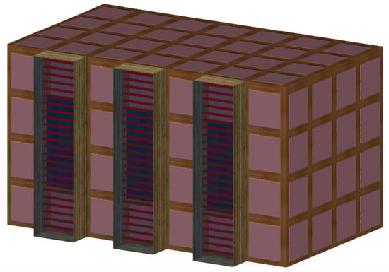
Figure 1.
Compartment, double skin facade (DSF) structure, DSF glasses and Venetian-type blinds.
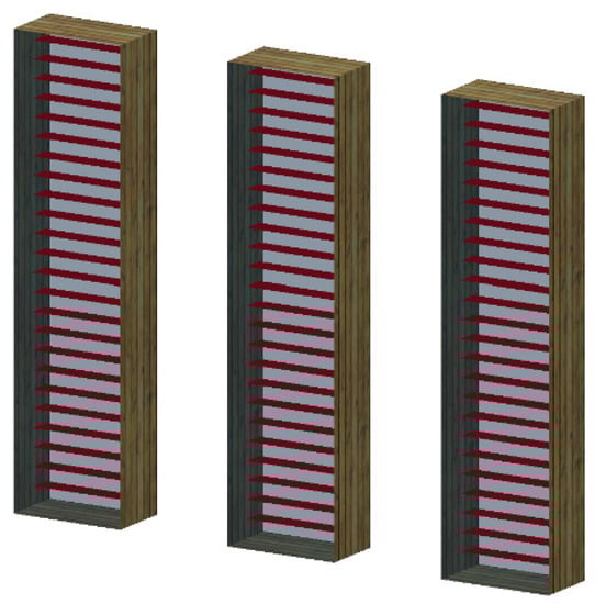
Figure 2.
DSF structure, DSF glasses and Venetian-type blind.

Figure 3.
Venetian-type blind.
The study was done for typical winter day conditions considering an average number of 8 occupants. The occupation cycle of the virtual chamber is the following:
- 08:00 a.m. to 12:00 p.m., during the morning time, is occupied by 8 persons;
- 12:00 p.m. to 14:00 (2:00 p.m.) is not occupied (lunch time);
- 14:00 (2:00 p.m.) to 18:00 (6:00 p.m.), during the afternoon time, is occupied by 8 persons.
The metabolic rate of 1.2 Met (70 W/m2) and the clothing insulation level of 1 clo were used in this work [28].
The DSF system and the virtual chamber were subjected to the airflow rates presented in Table 1. The airflow rate during the night and during the lunch time considers one air change rate between the space and the outdoors (out). In the morning and in the afternoon time, when the virtual chamber is occupied, the considered airflow rates, which come from the outside environment to the DSF system, then to the virtual camera and from there to the outside environment, are the following:

Table 1.
Airflow rate used in each case studied.
- 4Q (0.0389 m3/s), airflow rate in accordance to the standards acceptable for four occupants;
- 6Q (0.0583 m3/s), airflow rate in accordance to the standards acceptable for six occupants;
- 8Q (0.0778 m3/s), airflow rate in accordance to the standards acceptable for eight occupants.
In this study a pre-programming horary control was implemented. This methodology considers ten case studies divided in three methodologies (see Figure 4, Figure 5 and Figure 6 and Table 2):
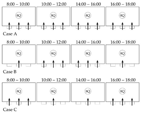
Figure 4.
Scheme of the pre-programming horary control of the DSF system, when the airflow rate is constant and the number of DSF to operate is variable.
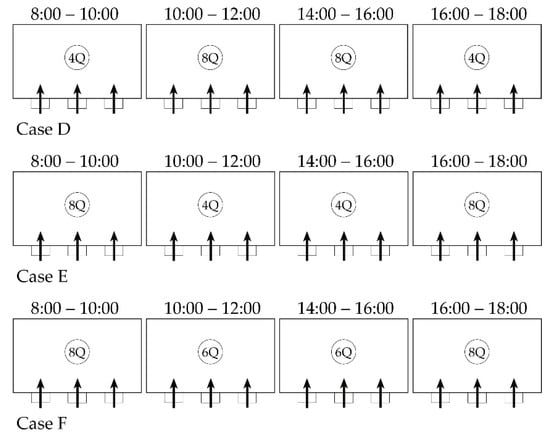
Figure 5.
Scheme of the pre-programming horary control of the DSF system, when the airflow rate is variable and the number of DSF to operate is constant.
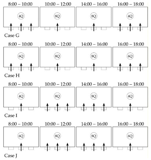
Figure 6.
Scheme of the pre-programming horary control of the DSF system, when the airflow rate is variable and the number of DSF to operate is variable.
Table 2.
DSF used in each case study.
In the numerical simulation, input and output data were considered. The input data were as follows:
- The buildings geometry (introduced in a three-dimensional design software using a computational aided design (CAD) methodology);
- The boundary conditions (evolution of external environmental variables during the day);
- The thermal properties of the materials of the opaque, transparent and interior bodies;
- The geographical conditions (location of the building on the earth’s surface);
- The initial conditions. In order to consider the building thermal capacity and, consequently, the temperature distribution similar to a real building in similar conditions, the previous days are also considered in the numerical simulation, and the initial conditions are similar to the external environment conditions; the process stops when the temperature in the day final field is similar to the day initial field;
- The occupation cycle (using the distribution of people during the day in each space);
- The occupant’s clothing and activity levels;
- The air ventilation topologies (using the distribution of airflow during the day in each space);
- Other conditions.
The output data are as follows:
- The several heat and mass coefficients;
- The solar radiation received by each surface of the building envelope;
- The mass and temperature fields;
- The thermal comfort evaluated by the PMV/PPD indexes;
- The indoor air quality evaluated by the carbon dioxide concentration;
- The energy consumption level;
- Others variables.
4. Results and Discussion
In this section, the indoor air quality, the thermal comfort and the uncomfortable hours are presented. In this study, ten case studies, divided into three groups, were analyzed as follows:
- pre-programming horary control of the DSF system, when the airflow rate is constant and the number of DSF to operate is variable;
- pre-programming horary control of the DSF system, when the airflow rate is variable and the number of DSF to operate is constant;
- pre-programming horary control of the DSF system, when the airflow rate is variable and the number of DSF to operate is variable.
4.1. Indoor Air Quality
In this section, the indoor air quality was evaluated. In these studied cases, the mixing ventilation was applied and the carbon dioxide concentration, used as indicator of the indoor air quality, was applied.
According to the mass balance integral equation (carbon dioxide concentration and water vapor) presented earlier, this numerical simulation takes into account the inlet mass from the outdoor environment to the indoor environment, the outlet mass from the indoor environment to the outdoor environment and the mass generation in the human breathing process to the indoor environment. The mass inlet and the mass generation are well mixing in the occupied space. When the mass inlet is higher than the mass outlet, the mass in the space increases, and when the opposite is verified, the mass in the space decreases. The inlet airflow, equal to the outlet airflow, is responsible for the evolution of the mass. Thus, when the airflow rate increases or the mass generation decreases, the mass decreases, and when the airflow rate decreases or the mass generation increases, the mass increases.
From Figure 7, Figure 8, Figure 9, Figure 10 and Figure 11, the evolution of the carbon dioxide concentration is presented for, respectively, the ten cases studied.
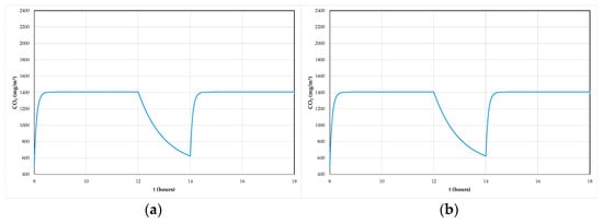
Figure 7.
Evaluation of carbon dioxide (CO2) concentration for Case A (a) and Case B (b).
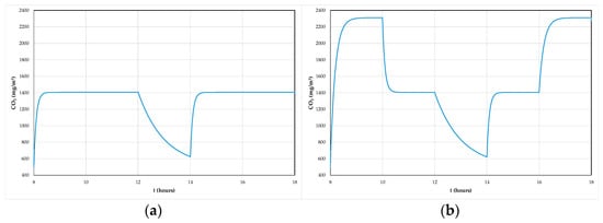
Figure 8.
Evaluation of carbon dioxide (CO2) concentration for Case C (a) and Case D (b).
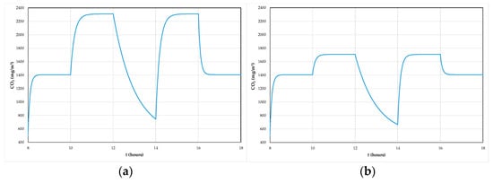
Figure 9.
Evaluation of carbon dioxide (CO2) concentration for Case E (a) and Case F (b).
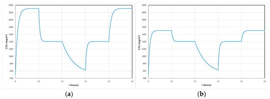
Figure 10.
Evaluation of carbon dioxide (CO2) concentration for Case G (a) and Case H (b).
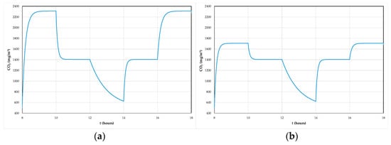
Figure 11.
Evaluation of carbon dioxide (CO2) concentration, for Case I (a) and Case J (b).
The indoor air quality was acceptable, according to ASHRAE 62.1 standard [33], for Cases A, B, C, F, H and J.
In Cases D, E, G and I the indoor air quality was not acceptable according to the ASHRAE 62.1 standard [33] as follows:
- In Cases D, G and I, it was only not acceptable in the first period of the morning and in the second period of the afternoon;
- In Case E only, it was not acceptable in the second period of the morning and in the first period of the afternoon.
However, the carbon dioxide concentration, in the non-acceptable periods, was near the acceptable value. Non-acceptable indoor air quality levels were verified for the lowest airflow rate.
4.2. Thermal Comfort
In this section the transmitted solar radiation and the virtual chamber, DSF system surfaces and indoor air temperatures were evaluated. The mean radiant temperate, calculated using the surrounding surfaces, the air velocity, the air temperature and relative humidity inside the virtual chamber were evaluated. This information, with the activity and clothing levels, was used to evaluate the thermal comfort level to which the occupants were subjected.
In Figure 12, the evaluation of transmitted solar radiation of the glazed surface for one DSF module is presented.
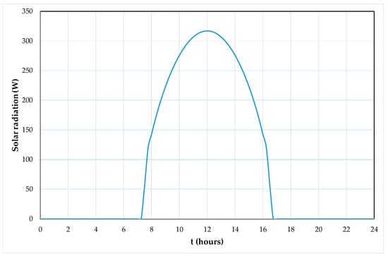
Figure 12.
Evaluation of transmitted solar radiation of the glazed surface of a DSF module.
In Figure 13, Figure 14, Figure 15, Figure 16, Figure 17, Figure 18, Figure 19, Figure 20, Figure 21 and Figure 22, the evolution of the air temperature of the outdoor environment, the indoor virtual chamber and the indoor DSF system are presented.
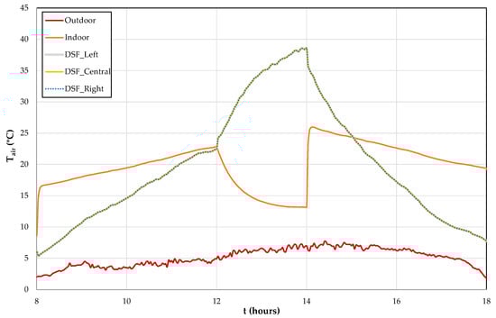
Figure 13.
Evaluation of air temperature (Tair) of the outdoor environment, indoor virtual chamber and indoor left, central and right DSF system, when the airflow rate is constant and the number of DSFs to operate is variable, for the Case A.
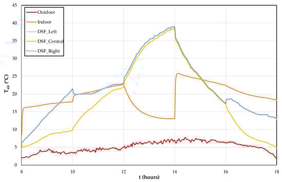
Figure 14.
Evaluation of air temperature (Tair) of the outdoor environment, indoor virtual chamber and indoor left, central and right DSF system, when the airflow rate is constant and the number of DSFs to operate is variable, for the Case B.
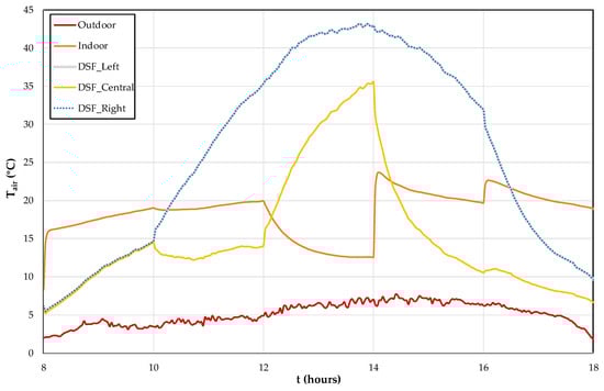
Figure 15.
Evaluation of air temperature (Tair) of the outdoor environment, indoor virtual chamber and indoor left, central and right DSF system, when the airflow rate is constant and the number of DSFs to operate is variable, for the Case C.
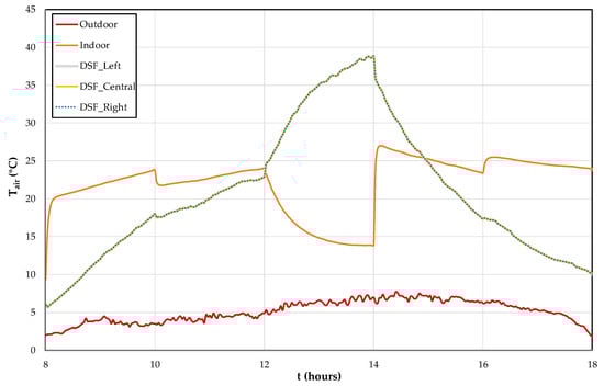
Figure 16.
Evaluation of air temperature (Tair) of the outdoor environment, indoor virtual chamber and indoor left, central and right DSF system, when the airflow rate is variable and the number of DSFs to operate is constant, for the Case D.
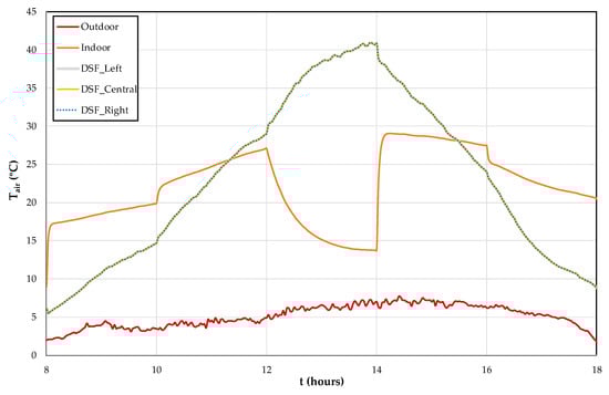
Figure 17.
Evaluation of air temperature (Tair) of the outdoor environment, indoor virtual chamber and indoor left, central and right DSF system, when the airflow rate is variable and the number of DSFs to operate is constant, for the Case E.
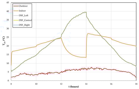
Figure 18.
Evaluation of air temperature (Tair) of the outdoor environment, indoor virtual chamber and indoor left, central and right DSF system, when the airflow rate is variable and the number of DSFs to operate is constant, for the Case F.
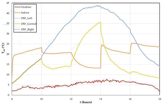
Figure 19.
Evaluation of air temperature (Tair) of the outdoor environment, indoor virtual chamber and indoor left, central and right DSF system, when the airflow rate is variable and the number of DSFs to operate is variable, for the Case G.
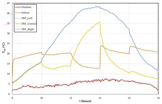
Figure 20.
Evaluation of air temperature (Tair) of the outdoor environment, indoor virtual chamber and indoor left, central and right DSF system, when the airflow rate is variable and the number of DSFs to operate is variable, for the Case H.
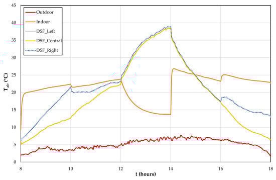
Figure 21.
Evaluation of air temperature (Tair) of the outdoor environment, indoor virtual chamber and indoor left, central and right DSF system, when the airflow rate is variable and the number of DSFs to operate is variable, for the Case I.
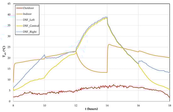
Figure 22.
Evaluation of air temperature (Tair) of the outdoor environment, indoor virtual chamber and indoor left, central and right DSF system, when the airflow rate is variable and the number of DSFs to operate is variable, for the Case J.
The outdoor air temperature, which varied between zero and eight degrees, presented the lowest value of air temperature. The air temperature inside the DSF system presented the highest values, mainly at noon. In the beginning of the morning and in the end of the afternoon, the air temperature inside the DSF system presented values near the outside air temperature. The air temperature inside the virtual chamber presented, in general, a more constant value as follows:
- In the morning there was an increase, due to the increase of energy transferred from the DSF system, associated with the increase of the incident solar radiation in the DSF system;
- At noon there was a decrease, due to the air change rate from the external environment;
- In the afternoon, there was a sudden increase and then a decrease during the afternoon, due to the decrease of energy transferred from the DSF system, associated with the decrease of the incident solar radiation in the DSF system.
In this work, the air temperature inside the right DSF was always equal to the left DSF. However, the air temperature inside the central DSF only was equal to the other two DSFs when all DSFs were used simultaneously, with similar conditions throughout the day.
The Cases A, B and C were verified when the airflow rate was constant and the number of DSF to operate was variable.
Case A (see Figure 13) was used as reference. The three DSF systems were working during the morning and afternoon with a maximum airflow rate. Thus, the DSF internal air temperature was equal for the three DSF systems.
When working only one central DSF system in the beginning of the morning, Case B, the internal DSF air temperature of the lateral DSF was higher than the air temperature of the central DSF, in the morning and in the final period of the afternoon. However, when working three DSF systems in the beginning of the morning and in second period of the afternoon, Case C, the internal DSF air temperature of the lateral DSF was lower than the air temperature of the central DSF during the second period of the morning, at noon and all afternoon.
The Cases D, E and F were verified when the airflow rate was variable and the number of DSFs to operate was constant.
When the airflow rate decreased, more energy was transported from the DSF system to the virtual chamber. Thus, when the airflow rate decreased, the internal air DSF temperature increased and the internal air of the virtual chamber temperature increased.
In these Cases, the evolution of internal air DSF temperature of the lateral DSF was equal to the central DSF. However, the slope of the internal air temperature evolution inside the DSF system was higher for the lowest airflow rate.
Finally, the Cases G, H, I and J were verified when the airflow rate was variable and the number of DSF to operate was variable. In these Cases, the results were a combination of the results presented before. Thus, in accordance with the obtained results:
- When working only one central DSF system the internal DSF air temperature of the lateral DSF is higher than the air temperature of the central DSF;
- When working three DSF systems, the internal DSF air temperature of the lateral DSF is lower than the air temperature of the central DSF;
- When the airflow rate decreases, the internal air DSF temperature increases, and the internal air virtual chamber temperature increases;
- The slope of the internal air temperature evolution inside the DSF system is higher for the lowest airflow rate.
The evolution of the virtual chamber internal air temperature is influenced by the DSF internal air temperature. This influence is detailed in Figure 23, where all evolutions of the virtual chamber internal air temperatures are compared.
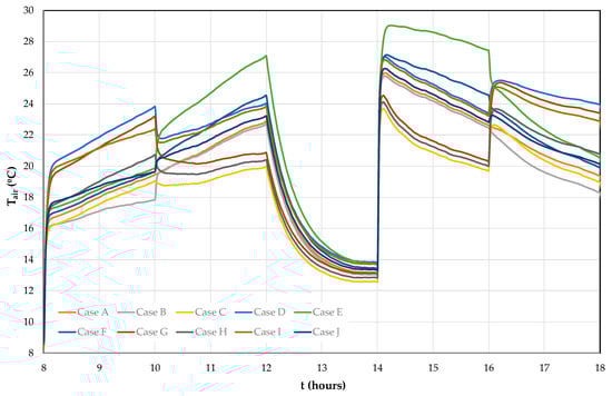
Figure 23.
Evaluation of virtual chamber air temperature (Tair) for all cases.
Figure 23 shows that Case E presented the highest value of the virtual chamber internal air temperature in the second period of the morning and in the first period of the afternoon. Case D presented the highest value of the virtual chamber internal air temperature in the first period of the morning and in the second period of the afternoon. Case C presented the smallest value of the virtual chamber internal air temperature in the second period of the morning and in the first period of the afternoon. Case B presented the highest value of the virtual chamber internal air temperature in the first period of the morning and in the second period of the afternoon. In order to promote the best thermal comfort conditions, it is necessary to increase the indoor air temperature during the entire day. However, this fact is analyzed in detail through the cold uncomfortable hours in the next section.
From Figure 24, Figure 25, Figure 26, Figure 27 and Figure 28 the evolution of the predicted mean vote index for the ten cases analyzed is presented.
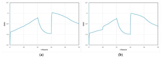
Figure 24.
Evaluation of predicted mean vote (PMV) index for the Case A (a) and Case B (b).
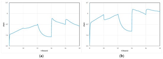
Figure 25.
Evaluation of predicted mean vote (PMV) index for the Case C (a) and Case D (b).
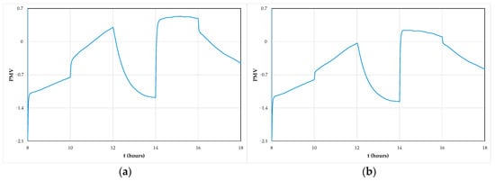
Figure 26.
Evaluation of predicted mean vote (PMV) index for the Case E (a) and Case F (b).
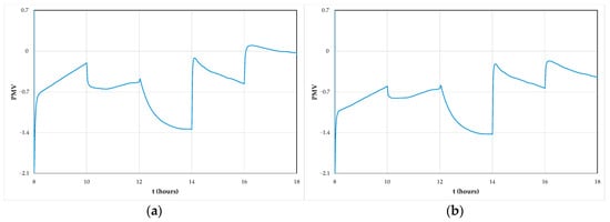
Figure 27.
Evaluation of predicted mean vote (PMV) index for the Case G (a) and Case H (b).
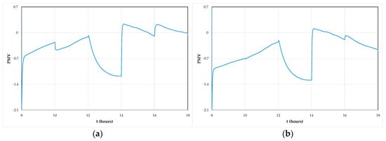
Figure 28.
Evaluation of predicted mean vote (PMV) index for the Case I (a) and Case J (b).
The thermal comfort level, evaluated by the PMV index, are functions of the mean air temperature, mean air relative humidity, mean radiant temperature, mean indoor air velocity, clothing level and activity level to which the occupants are subjected.
In general, during the second period of the morning and in the first period of the afternoon, the acceptable thermal comfort conditions were guaranteed. Cases D, G and I presented, in general, acceptable thermal comfort conditions, according to category C of ISO 7730 [28], during occupancy.
In general, the thermal comfort level was obtained by negative PMV values. Only in a few cases did the PMV index present positive values, although with PMV index values lower than 0.7.
4.3. Uncomfortable Hours
In Table 3 and Table 4 are presented, respectively, the air quality uncomfortable hours (AQUH) and the cold uncomfortable hours (CUH). In Table 5 is presented the total of uncomfortable hours given by the sum of AQUH and CUH. The percentage of variation of total uncomfortable hours in relation to Case A (reference) of the other nine cases studied is presented in Table 6.
Table 3.
Air quality uncomfortable hours in each case studied.
Table 4.
Cold uncomfortable hours in each case studied.
Table 5.
Air quality uncomfortable hours (AQUH) and cold uncomfortable hours (CUH) in each case study.
Table 6.
Percentage of variation of total of uncomfortable hours of the others nine cases relative to Case A (Reference Case).
The obtained results show that the air quality uncomfortable hours was highest for cases D, E, G and I. In these cases, associated with low airflow rate, the cold uncomfortable hours presented the lowest values. Case J presented the lowest uncomfortable hours. However, Cases A, D, F, G, H and I presented uncomfortable hours lower than 5 h. The influence of the airflow rate in the uncomfortable hours was more important than the influence of the DSF operating methodology. However, the simultaneous influence of the two variables showed that the uncomfortable hours presented the best results associated with the best levels of thermal comfort and indoor air quality. Thus, the following statements can be made:
- When the number of DSFs to operate decreases in the first period of the morning and in the second period of the afternoon, Cases A and B, the uncomfortable hours increase;
- When the number of DSFs to operate decreases in the second period of the morning and in the first period of the afternoon, Cases A and C, the uncomfortable hours increase. However, the decrease in the second period of the morning and in the first period of the afternoon presents higher uncomfortable hours than the decrease in the first period of the morning and in the second period of the afternoon;
- When the airflow rate decreases 50% in the first period of the morning and in the second period of the afternoon, Cases A and D, the uncomfortable hours decrease;
- When the airflow rate decreases 50% in the second period of the morning and in the first period of the afternoon, Cases A and E, the uncomfortable hours increase;
- When the airflow rate decreases 25% in the second period of the morning and in the first period of the afternoon, Cases A and F, the uncomfortable hours decrease. This decrease is more significant, because the air quality uncomfortable hours also decrease;
- When the airflow rate decreases 25% in the first period of the morning and in the second period of the afternoon, Cases B and I, the uncomfortable hours decrease;
- When the airflow rate decreases 25% in the first period of the morning and in the second period of the afternoon, Cases B and J, the uncomfortable hours decrease significantly;
- When the airflow rate decreases 50% in the first period of the morning and in the second period of the afternoon, Cases C and G, the uncomfortable Hours decrease. However, the decrease of the uncomfortable hours in the Case I is higher than in the Case G;
- When the airflow rate decreases 25% in the first period of the morning and in the second period of the afternoon, Cases C and H, the uncomfortable hours decrease significantly. However, the decrease of the uncomfortable hours for Case J is higher than for Case H;
- When the airflow rate decreases 25% in the first period of the morning and in the second period of the afternoon, Cases D and E, the uncomfortable hours are lower than when the airflow rate decreases 50% in the second period of the morning and in the first period of the afternoon;
- When the number of DSF to operate decreases in the first period of the morning and in the second period of the afternoon, Cases D and I, the uncomfortable hours increase slightly;
- When the airflow rate increases from 0.0389 m3/s (4Q) to 0.0583 m3/s (6Q) in the second period of the morning and in the first period of the afternoon, Cases E and F, the uncomfortable hours decrease;
- When the number of DSFs to operate decreases in the second period of the morning and in the first period of the afternoon, Cases G, H, I and J, the uncomfortable hours are higher than when the number of DSFs to operate decreases in the second period of the morning and in the first period of the afternoon.
According to the results in Table 6, it appears that Cases B, C and E showed a large increase in total of uncomfortable hours (45.4%, 72.4% and 62.1%, respectively), especially in Cases B and C due to increased cold uncomfortable hours and, in Case E, due to increased uncomfortable indoor air quality hours. Cases F and J had the greatest decrease in total of uncomfortable hours, respectively, of −21.6% and −37.2%, due to the decrease in cold uncomfortable hours. Compared to Case A (reference), Case J presented the best result regarding total uncomfortable hours.
In this work, the comfort, the indoor thermal comfort and the indoor air quality were evaluated in mixing ventilation conditions. Here, the mean value of comfort conditions was obtained. In future works, using the coupling of the computational fluid dynamics and human thermal response numerical models, the evaluation of the comfort conditions to which each occupant is subjected, for different ventilations systems, will be evaluated.
5. Conclusions
A comparative study of a clean technology based on DSF used in winter conditions in the occupied buildings comfort improvement is presented in this study. A virtual chamber occupied with eight persons and equipped with a system of three DSF, in the outdoor environment, and a mixing ventilation system, in the indoor environment, is used on a winter day. A pre-programming horary control methodology is developed and applied when the airflow rate is constant and the number of DSFs to operate is variable, when the airflow rate is variable and the number of DSFs to operate is constant and when the airflow rate is variable and the number of DSFs to operate is variable. The indoor air quality, the thermal comfort and the uncomfortable hours are evaluated.
In general, the indoor air quality is acceptable. Non-acceptable values, however, near the acceptable values, are verified only for the lowest airflow rate.
In general, the air temperature inside the DSF system increases during the morning period, then increases significantly during noon and finally decreases during the afternoon period. The increase is due to the solar radiation and the extra increase during noon is due to lack of ventilation.
When the pre-programing horary control of the DSF to operate and the airflow rate are variable, as in Cases E and D, the air temperature of the virtual chamber presents higher values than when the DSF to operate is variable and the airflow rate is constant, as in Cases B and C.
The decrease of the number of DSFs to operate implies that the uncomfortable hours increase. The decrease of the number of DSFs to operate in the second period of the morning and in the first period of the afternoon implies higher uncomfortable hours than the decrease of the number of DSFs to operate in the first period of the morning and in the second period of the afternoon.
The 50% decrease in the airflow rate, mainly in the first period of the morning and in the second period of the afternoon, implies the decrease of the uncomfortable hours. However, the 25% decrease in the airflow rate implies a significant decrease of the uncomfortable hours.
Case J presents the greatest reduction in total uncomfortable hours, namely −37.5% compared to Case A (reference), essentially due to the reduction in cold uncomfortable hours. This Case represents the best compromise that is obtained, in this work, with a pre-programming horary control of the airflow rate variation and the DSF to operate throughout the day.
Author Contributions
All authors contributed equally in the preparation of this manuscript. All authors have read and agreed to the published version of the manuscript.
Funding
The authors would like to acknowledge the project (SAICT-ALG/39586/2018) from Algarve Regional Operational Program (CRESC Algarve 2020), under the PORTUGAL 2020 Partnership Agreement, through the European Regional Development Fund (ERDF) and the National Science and Technology Foundation (FCT).
Institutional Review Board Statement
Not applicable.
Informed Consent Statement
Not applicable.
Data Availability Statement
Data sharing not applicable.
Conflicts of Interest
The authors declare no conflict of interest.
References
- Shameri, M.; Alghoul, M.; Sopian, K.; Zain, M.; Elayeb, O. Perspectives of double skin façade systems in buildings and energy saving. Renew. Sustain. Energ. Rev. 2011, 15, 1468–1475. [Google Scholar] [CrossRef]
- Carlos, J.; Corvacho, H.; Silva, P.; Castro-Gomes, J. Modelling and simulation of a ventilated double window. Appl. Therm. Eng. 2011, 31, 93–102. [Google Scholar] [CrossRef]
- Hashemi, N.; Fayaz, R.; Sarshar, M. Thermal behaviour of a ventilated double skin façade in hot arid climate. Energy Build. 2010, 42, 1823–1832. [Google Scholar] [CrossRef]
- Ghaffarianhoseini, A.; Ghaffarianhoseini, A.; Berardi, U.; Tookey, J.; Li, D.; Kariminia, S. Exploring the advantages and challenges of double-skin façades (DSFs). Renew. Sustain. Energy Rev. 2016, 60, 1052–1065. [Google Scholar] [CrossRef]
- Poirazis, H. Double Skin Façades for Office Buildings–Literature Review; Report EBD-R–04/3; Department of Construction and Architecture, Lund University: Lund, Sweden, 2004. [Google Scholar]
- Lucchino, E.; Goia, F.; Lobaccaro, G.; Chaudhary, G. Modelling of double skin facades in whole-building energy simulation tools: A review of current practices and possibilities for future developments. Build. Simul. 2019, 12, 3–27. [Google Scholar] [CrossRef]
- Xue, F.; Li, X. A fast assessment method for thermal performance of naturally ventilated double-skin façades during cooling season. Sol. Energy 2015, 114, 303–313. [Google Scholar] [CrossRef]
- Hazem, A.; Ameghchouche, M.; Bougriou, C. A numerical analysis of the air ventilation management and assessment of the behavior of double skin facades. Energy Build. 2015, 102, 225–236. [Google Scholar] [CrossRef]
- Lee, J.; Chang, D. Influence on vertical shading device orientation and thickness on the natural ventilation and acoustical performance of a double skin façade. Procedia Eng. 2015, 118, 304–309. [Google Scholar] [CrossRef]
- Lee, J.; Alshayeb, M.; Chang, D. A study of shading device configuration on the natural ventilation efficiency and energy performance of a double skin façade. Procedia Eng. 2015, 118, 310–317. [Google Scholar] [CrossRef]
- Parra, J.; Guardo, A.; Egusquiza, E.; Alavedra, P. Thermal performance of ventilated double skin façades with venetian blinds. Energies 2015, 8, 4882–4898. [Google Scholar] [CrossRef]
- Li, Y.; Darkwa, J.; Su, W. Investigation on thermal performance of an integrated phase change material blind system for double skin façade buildings. Energy Procedia 2019, 158, 5116–5123. [Google Scholar] [CrossRef]
- Ziasistani, N.; Fazelpour, F. Comparative study of DSF, PV-DSF and PV-DSF/PCM building energy performance considering multiple parameters. Sol. Energy 2019, 187, 115–128. [Google Scholar] [CrossRef]
- Fazelpour, F.; Soltani, N.; Markarian, E.; Khezerloo, H. Impact of multiple parameters on energy performance of PV-DSF buildings. Proceedings 2018, 2, 1487. [Google Scholar] [CrossRef]
- Fatnassi, S.; Abidi-Saad, A.; Maad, R.; Polidori, G. Numerical study of spacing and alternation effects of parietal heat sources on natural convection flow in a DSF-channel: application to BIPV. Int. J. Heat Mass Trans. 2018, 54, 3617–3629. [Google Scholar] [CrossRef]
- Wang, Y.; Chen, Y.; Li, C. Airflow modeling based on zonal method for natural ventilated double skin façade with Venetian blinds. Energy Build. 2019, 191, 211–223. [Google Scholar] [CrossRef]
- Zhang, T.; Yang, H. Flow and heat transfer characteristics of natural convection in vertical air channels of double-skin solar façades. Appl. Energy 2019, 242, 107–120. [Google Scholar] [CrossRef]
- Blanco, J.; Arriaga, P.; Rojí, E.; Cuadrado, J. Investigating the thermal behavior of double-skin perforated sheet façades: Part A: Model characterization and validation procedure. Build. Environ. 2014, 82, 50–62. [Google Scholar] [CrossRef]
- Kim, D.; Cox, S.; Cho, H.; Yoon, J. Comparative investigation on building energy performance of double skin façade (DSF) with interior or exterior slab blinds. J. Build. Eng. 2018, 20, 411–423. [Google Scholar] [CrossRef]
- Kuznik, F.; Catalina, T.; Gauzere, L.; Woloszyn, M.; Roux, J.-J. Numerical modelling of combined heat transfers in a double skin façade – Full-scale laboratory experiment validation. Appl. Therm. Eng. 2011, 31, 3043–3054. [Google Scholar] [CrossRef][Green Version]
- Conceição, E.; Lúcio, M. Numerical study of the thermal efficiency of a school building with complex topology for different orientations. Indoor Built Environ. 2008, 18, 41–51. [Google Scholar] [CrossRef]
- Conceição, E.; Lúcio, M.; Lopes, M. Application of an indoor greenhouse in the energy and thermal comfort performance in a kindergarten school building in the south of Portugal in winter conditions. WSEAS Trans. Environ. Dev. 2008, 4, 644–654. [Google Scholar]
- Conceição, E.; Gomes, J.; Awbi, H. Influence of the airflow in a solar passive building on the indoor air quality and thermal comfort levels. Atmosphere 2019, 10, 766. [Google Scholar] [CrossRef]
- Conceição, E.; Lúcio, M. Numerical simulation of the application of solar radiant systems, internal airflow and occupants’ presence in the improvement of comfort in winter conditions. Buildings 2016, 6, 38. [Google Scholar] [CrossRef]
- Conceição, E.; Lúcio, M.; Ruano, A.; Crispim, E. Development of a temperature control model used in HVAC systems in school spaces in Mediterranean climate. Build. Environ. 2009, 44, 871–877. [Google Scholar] [CrossRef]
- Conceição, E.; Gomes, J.; Ruano, A. Application of HVAC systems with control based on PMV index in university buildings with complex topology. IFAC PapersOnLine. 2018, 51, 20–25. [Google Scholar] [CrossRef]
- Fanger, P. Thermal Comfort: Analysis and Applications in Environmental Engineering; Danish Technical Press: Copenhagen, Denmark, 1970. [Google Scholar]
- ISO 7730. Ergonomics of the Thermal Environments—Analytical Determination and Interpretation of Thermal Comfort Using Calculation of the PMV and PPD Indices and Local Thermal Comfort Criteria; International Standard Organization: Geneva, Switzerland, 2005. [Google Scholar]
- ANSI/ASHRAE Standard 55. Thermal Environmental Conditions for Human Occupancy; American Society of Heating, Refrigerating and Air-Conditioning Engineers: Atlanta, GA, USA, 2013. [Google Scholar]
- Asif, A.; Zeeshan, M.; Jahanzaib, M. Indoor temperature, relative humidity and CO2 levels assessment in academic buildings with different heating, ventilation and air-conditioning systems. Build. Environ. 2018, 133, 83–90. [Google Scholar] [CrossRef]
- Laverge, J.; Van Den Bossche, N.; Heijmans, N.; Janssens, A. Energy saving potential and repercussions on indoor air quality of demand controlled residential ventilation strategies. Build. Environ. 2011, 46, 1497–1503. [Google Scholar] [CrossRef]
- Conceição, E.Z.; Lúcio, M.J.; Vicente, V.D.; Rosão, V.C. Evaluation of Local Thermal Discomfort in a Classroom Equipped with Crossed Ventilation. Int. J. Vent. 2008, 7, 267–277. [Google Scholar]
- ANSI/ASHRAE Standard 62-1. Ventilation for Acceptable Indoor Air Quality; American Society of Heating, Refrigerating and Air-Conditioning Engineers: Atlanta, GA, USA, 2016. [Google Scholar]
- Olesen, B.; Parsons, K. Introduction to thermal comfort standards and to the proposed new version of EN ISO 7730. Energy Build. 2002, 34, 537–548. [Google Scholar] [CrossRef]
- Van der Linden, K.; Boerstra, A.; Raue, A.; Kurvers, S. Thermal indoor climate building performance characterized by human comfort response. Energy Build. 2002, 34, 737–744. [Google Scholar] [CrossRef]
- Conceição, E.; Lúcio, M.; Awbi, H. Comfort and airflow evaluation in spaces equipped with mixing ventilation and cold radiant floor. Build. Simul. 2013, 6, 51–67. [Google Scholar] [CrossRef]
- Conceição, E.; Lúcio, M. Numerical simulation of passive and active solar strategies in buildings with complex topology. Build. Simul. 2010, 3, 245–261. [Google Scholar] [CrossRef]
Publisher’s Note: MDPI stays neutral with regard to jurisdictional claims in published maps and institutional affiliations. |
© 2021 by the authors. Licensee MDPI, Basel, Switzerland. This article is an open access article distributed under the terms and conditions of the Creative Commons Attribution (CC BY) license (http://creativecommons.org/licenses/by/4.0/).