On the Stability of the Euler–Poisson Dark-Fluid Model

Abstract

We present a stability analysis of a dark-fluid model described as a non-relativistic, rotating, non-viscous, self-gravitating fluid. We assume there is spherical symmetry and model the matter using a polytropic equation of state. The resulting coupled nonlinear partial differential equation system is solved using a self-similar ansatz known from the Guderley–Landau–Stanyukovich problem. We find that three of the four Lyapunov exponents are negative, while only one is positive. This indicates the existence of one unstable direction and three contracting directions in phase space. The single positive exponent is relatively small, suggesting that the self-similar solution is only weakly unstable and remains dynamically robust over the investigated interval.

1. Introduction

By employing various symmetries, one can successfully solve a wide variety of dynamical systems described by nonlinear partial differential equations (PDEs). One particularly common and useful type of symmetry is self-similarity. Numerous physically relevant self-similar solutions have been found since Gottfried Guderley’s famous discovery of spherically symmetric self-similar solutions for an imploding gas collapsing toward the center [1]. In this paper, we use the self-similar solutions introduced independently by Leonid Ivanovich Sedov and Sir Geoffrey Ingram Taylor during the 1940s [2,3].

Although such models have been well known for decades, they continue to attract considerable attention. This ansatz has already been applied successfully in several contexts, including heat conduction [4], the three-dimensional Navier–Stokes and Euler equations [5], and star formation [6]. The concept of self-similarity also has a wide range of applications in general relativity. Homothetic solutions were first introduced by Cahill and Taub [7] and have been studied extensively in connection with gravitational collapse [8] and asymptotic cosmological solutions [9].

This perspective is particularly relevant in astrophysical and cosmological settings, where some of the most fundamental open problems concern the dark sector. One possible approach is the dark-fluid concept, which seeks to describe both dark matter and dark energy within a single continuous classical medium [10]. In our previous studies, we developed and investigated a cosmological model based on hydrodynamics [11]. The dynamics of the dark-fluid-like medium are governed by a coupled nonlinear system of partial differential equations. In our model, we studied one of the simplest dark-fluid materials described by a linear equation of state (EoS). The Euler equation governs fluid dynamics, whereas the associated gravitational field is determined through the Poisson equation. We found time-dependent scaling solutions for the velocity, density, and gravitational fields that could serve as candidates for describing the evolution of gravitationally coupled dust-like dark matter within a Newtonian cosmological framework. Our present goal is to provide a stability analysis of our model and derive the Lyapunov exponents.

2. The Model

We consider a set of coupled non-linear partial differential equations, which describe the non-relativistic dynamics of a compressible, self-gravitating, rotating fluid with zero thermal conductivity and zero viscosity, in radial spherical coordinates.

The first governing equation is the continuity equation. The second is the Euler equation, which includes the pressure term derived from the EoS, the radial component of the external force density, and an effective rotational term on the right-hand side. Here, $\omega$ is a dimensionless parameter describing the magnitude of rotation, and $\theta$ is the polar angle. We assume that the rotation is slow enough that a spherically symmetric leading-order description remains applicable; i.e., the rotational energy is negligible compared with the gravitational energy. The third equation is the Poisson equation for the gravitational field.

$$\begin{array}{cc}\hfill {\partial }_t\rho +\left({\partial }_r\rho \right)u+\left({\partial }_{r}u\right)\rho +{\displaystyle \frac{2u\rho }{r}}& =0,\hfill \end{array}$$

(1a)

$$\begin{array}{cc}\hfill {\partial }_{t}u+\left(u{\partial }_r\right)u& =-{\displaystyle \frac{1}{\rho }}{\partial }_{r}P-{\partial }_r\mathsf{\Phi }+{\displaystyle \frac{\sin \theta {\omega }^{2}r}{t^2}},\hfill \end{array}$$

(1b)

$$\begin{array}{cc}\hfill 2{\partial }_r\mathsf{\Phi }+r{\partial }_{rr}\mathsf{\Phi }& =4\pi Gr\rho .\hfill \end{array}$$

(1c)

Here, the dynamical variables are $\rho =\rho (r,t)$, $u=u(r,t)$, $\mathsf{\Phi }=\mathsf{\Phi }(r,t)$, and $P=P(r,t)$, denoting the density, radial velocity, gravitational potential, and pressure, respectively. We apply the linear EoS

$$P\left(\rho \right)=w{\rho }^n,n=1.$$

(2)

More information about the model can be found in [12]. Several forms of the EoS are available in astrophysics, and polytropic ones have been used successfully in the past; see, for example, Emden’s classical book [13]. Equations of state with negative pressure of this type are widely used in dark-fluid cosmology, most notably in the Chaplygin and generalized Chaplygin gas models [14,15,16]. In Equation (2), the parameter w may vary depending on the type of matter governing the system’s evolution. Traditionally, $w=0$ corresponds to the EoS of ordinary non-relativistic matter or cold dust. In this paper, we choose $w=-1$ as a simple phenomenological case within the present dark-fluid framework. The adiabatic speed of sound can be evaluated from Equation (2), and it is straightforward to show that it is constant. Note that, in the calculations below, the geometrized unit system ($c=1$, $G=1$) is used.

One can find semi-analytic solutions to the equations by applying the long-established self-similar ansatz developed by Sedov and Taylor [2,3], which can be expressed in the following form:

$$\begin{array}{c}u(r,t)=t^{-\alpha }f\left({\displaystyle \frac{r}{t^{\beta }}}\right),\end{array}$$

(3a)

$$\begin{array}{c}\rho (r,t)=t^{-\gamma }g\left({\displaystyle \frac{r}{t^{\beta }}}\right),\end{array}$$

(3b)

$$\begin{array}{c}\mathsf{\Phi }(r,t)=t^{-\delta }h\left({\displaystyle \frac{r}{t^{\beta }}}\right),\end{array}$$

(3c)

where t denotes time and r the radial coordinate. One can see that all shape functions $(f,g,h)$ depend only on the combination $r{t}^{-\beta }$; therefore, we introduce the self-similarity variable $\zeta$. The variable $\zeta$ is dimensionless in geometrized units. The exponents $\alpha$, $\beta$, $\gamma$, and $\delta$ are called similarity exponents and have clear physical meanings. In particular, $\beta$ characterizes the temporal spreading of the spatial profile when $\beta >0$, or contraction when $\beta <0$. The remaining exponents describe the temporal scaling of the amplitudes of the corresponding fields. The similarity density profile $g\left(\eta \right)$ is restricted by the physical admissibility condition $g\left(\eta \right)\ge 0$.

A general description of the properties of these types of scaling solutions can be found in our previous publication [11]. Thus, we have calculated the relevant time and space derivatives of the shape functions and substituted them into the equations in Equation (1). We obtained the following numerical value for the exponents $\alpha =0$, $\beta =1$, $\gamma =2$, and $\delta =0$ for both the non-rotating and the rotating cases. These exponent values indicate a spreading spatial profile for the relevant dynamical variables. In this sense, the self-similar behavior may be interpreted as expansion-like at large astrophysical or cosmological scales.

By substituting the obtained numerical values of the similarity exponents, we have reduced the induced PDE system into an ordinary differential equation (ODE) system that depends only on the $\zeta$ independent variable. We found that the obtained equation system has the following form:

$$\begin{array}{cc}\hfill \zeta {\left[f\left(\zeta \right)g\left(\zeta \right)\right]}^{\prime }+2f\left(\zeta \right)g\left(\zeta \right)& =2g\left(\zeta \right)+{\zeta }^2{g}^{\prime }\left(\zeta \right),\hfill \end{array}$$

(4a)

$$\begin{array}{cc}\hfill -\zeta f^{\prime }\left(\zeta \right)+f^{\prime }\left(\zeta \right)f\left(\zeta \right)& =-{\displaystyle \frac{w{g}^{\prime }\left(\zeta \right)}{g\left(\zeta \right)}}-h^{\prime }\left(\zeta \right)+\zeta {\omega }^2\sin \theta ,\hfill \end{array}$$

(4b)

$$\begin{array}{cc}\hfill 2h^{\prime }\left(\zeta \right)+h^{″}\left(\zeta \right)\zeta & =4\pi g\left(\zeta \right)\zeta .\hfill \end{array}$$

(4c)

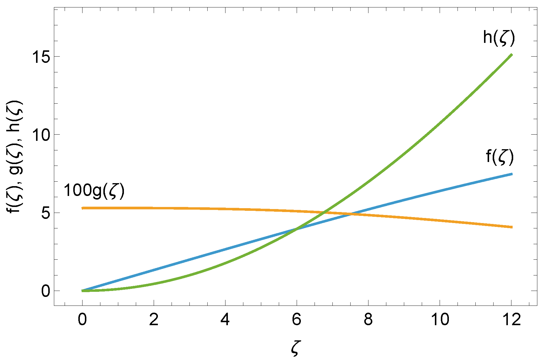
Unfortunately, the presented ordinary differential equation system Equation (4) cannot be solved analytically. For linearized non-autonomous ordinary differential equation systems, the stationary point of the phase space can be found, and one can say something about the general asymptotic behavior of the solutions [17]. Nonetheless, there is no generally known method for non-linearized non-autonomous differential equation systems. Local existence for the Euler–Poisson Cauchy problem has been studied in the mathematical literature, including density profiles without compact support [18]. Here, we restrict our attention to a self-similar solution class, defined for the time interval where the similarity ansatz is regular. Therefore, it is a reasonable approach to solve the obtained ordinary differential equation system, Equation (4), numerically for a large number of parameter sets (based on physical considerations) to explore the behavior of the solution to the system with different boundary and initial conditions. One example of the numerical solution is shown in Figure 1.

Here, with respect to a specific parameter set and initial conditions, the velocity shape function $f\left(\zeta \right)$ is nearly linear after a short initial decrease. The function $g\left(\zeta \right)$ becomes asymptotically flat after a rapid rise, which is consistent with matter conservation. The final shape function, $h\left(\zeta \right)$, exhibits an increasing polynomial trend associated with the gravitational potential. To obtain sufficiently smooth numerical solutions, we solved the ODE system using the adaptive numerical integrator provided by Wolfram Mathematica 13.1 [19]. For all calculations, the integration limits were ${\zeta }_0=0.001$ and ${\zeta }_{\max }=40$, as in Ref. [12]. We considered the following ranges of initial conditions: $f\left({\zeta }_0\right)=0.005$–$0.5$ and $g\left({\zeta }_0\right)=0.001$–$0.1$, together with $h\left({\zeta }_0\right)=0$ and $h^{\prime }\left({\zeta }_0\right)=1$.

This choice of initial conditions reflects the physically reasonable assumption that the density profile satisfies $\mathcal{R}\left(g\right)\subset {\mathbb{R}}^{+}$ and remains finite. Some recent work suggests that dark fluid may have negative mass [20]. However, in the present model, this choice leads to singular solutions. Likewise, $\mathcal{R}\left(f\right)\subset {\mathbb{R}}^{+}$ corresponds to an initially radially expanding fluid. We observed numerically that if the initial values of $f\left(\zeta \right)$ and $g\left(\zeta \right)$ are chosen outside the ranges given above, the solution becomes singular. We also found that varying the initial condition associated with the gravitational potential does not qualitatively affect the time evolution of the system but instead only produces vertical shifts. Therefore, we set its initial value to zero.

3. The Stability of the Self-Similar Solution

The Sedov–von Neumann–Taylor self-similar ansatz for the Euler–Poisson system provides a powerful framework for analyzing non-linear gravitating fluid dynamics. By introducing an appropriate similarity variable, the original partial differential equations governing velocity, density, and gravitational potential can be reduced to a coupled system of ordinary differential equations. Even though this reduction substantially simplifies the mathematical structure of the original problem, it typically leads to a dynamical system that is explicitly dependent on the similarity variable, rendering it inherently non-autonomous.

The non-autonomous nature of Sedov-type self-similar Euler–Poisson equations has important consequences for stability analysis. Classical approaches based on autonomous fixed-point theory [21] or asymptotic Lyapunov [22] exponents rely on infinite-time limits and time-translation invariance, assumptions that are generally violated in self-similar configurations. In particular, the evolution variable in the reduced system does not represent physical time, and the dynamics often terminate at finite values corresponding to singularity formation, shock emergence, or loss of self-similarity [23]. As a result, stability must be understood in a finite-interval sense, along dynamically evolving solutions.

In this context, finite-time Lyapunov methods offer a natural and mathematically consistent approach to stability analysis. By quantifying the growth or decay of infinitesimal perturbations along a reference self-similar trajectory over a prescribed interval of the similarity variable, finite-time Lyapunov exponents capture transient instabilities and local sensitivity that are intrinsic to non-autonomous gravitational flows. This trajectory-based perspective is particularly well-suited to self-similar Euler–Poisson dynamics.

Motivated by these considerations, the stability properties of the self-similar Euler–Poisson system studied in this work are analyzed using finite-time Lyapunov exponents computed along the obtained reference solutions. This framework provides a quantitative measure of dynamical stability that remains valid in the absence of an autonomous structure, allowing for a systematic investigation of transient growth phenomena relevant to gravitational collapse and self-similar flow evolution. Thus, one should consider a general non-autonomous dynamical system of the form

$${\displaystyle \frac{\mathrm{d}\mathbf{x}}{\mathrm{d}\zeta }}=\mathbf{F}(\mathbf{x},\zeta ),\mathbf{x}\in {\mathbb{R}}^n\mathrm{and}\zeta \in {\mathbb{R}}^{+},$$

(5)

where $\mathbf{F}:{\mathbb{R}}^n\times \mathbb{R}\to {\mathbb{R}}^n$ is assumed to be sufficiently smooth to ensure the existence and uniqueness of solutions [24]. Let $\mathbf{x}(\zeta ;{\zeta }_0,{\mathbf{x}}_0)$ denote the solution satisfying the initial condition $\mathbf{x}\left({\zeta }_0\right)={\mathbf{x}}_0$. The corresponding flow, $\phi$, is defined as follows:

$${\phi }_{{\zeta }_0}^{\zeta }\left({\mathbf{x}}_0\right)=\mathbf{x}(\zeta ;{\zeta }_0,{\mathbf{x}}_0).$$

(6)

For non-autonomous systems, the flow satisfies, for any intermediate point $\tau$,

$${\phi }_{{\zeta }_0}^{\zeta }(\zeta ;{\zeta }_0,{\mathbf{x}}_0)={\phi }_{\tau }^{\zeta }(\zeta ;\tau ,{\phi }_{{\zeta }_0}^{\tau }(\tau ;{\zeta }_0,{\mathbf{x}}_0)).$$

(7)

Throughout this analysis, a single reference trajectory is selected by specifying ${\mathbf{x}}_0$ and integrating the system over a finite interval $[{\zeta }_0,{\zeta }_f]$. Let us consider a small perturbation $\delta \left(\zeta \right)$ from the reference trajectory $\mathbf{x}\left(\zeta \right)$, such as

$$\mathbf{x}\left(\zeta \right)\to \mathbf{x}\left(\zeta \right)+\delta \mathbf{x}\left(\zeta \right).$$

(8)

The evolution of the perturbation is governed by the variational equation

$${\displaystyle \frac{\mathrm{d}}{\mathrm{d}\zeta }}\delta \mathbf{x}=D_{\mathbf{x}}\mathbf{F}\left(\mathbf{x}\left(\zeta \right),\zeta \right)\delta \mathbf{x},$$

(9)

where $D_{\mathbf{x}}\mathbf{F}$ denotes the Jacobian matrix of the vector field evaluated along the reference solution. The solution to the differential equation, defined in Equation (9), can be expressed in terms of the fundamental matrix

$$\mathsf{\Phi }({\zeta }_0,\zeta )=D{\phi }_{{\zeta }_0}^{\zeta }(\zeta ;{\zeta }_0,{\mathbf{x}}_0),$$

(10)

which maps initial perturbations to their evolved values,

$$\delta \mathbf{x}\left(\zeta \right)=\mathsf{\Phi }(\zeta ,{\zeta }_0)\delta \mathbf{x}\left({\zeta }_0\right),$$

(11)

with the following properties

$$\begin{array}{cc}\hfill \mathsf{\Phi }(\zeta ,\tau )\mathsf{\Phi }(\tau ,{\zeta }_0)& =\mathsf{\Phi }(\zeta ,{\zeta }_0),\hfill \end{array}$$

(12)

$$\begin{array}{cc}\hfill \mathsf{\Phi }(\zeta ,\tau )& ={\mathsf{\Phi }}^{-1}(\tau ,\zeta ),\hfill \end{array}$$

(13)

$$\begin{array}{cc}\hfill \mathsf{\Phi }(\tau ,\tau )& =\widehat{I}.\hfill \end{array}$$

(14)

For a given initial perturbation direction $\delta {\mathbf{x}}_0$, the finite-time Lyapunov exponent can be defined as

$$\lambda (\zeta ,{\zeta }_0,\delta {\mathbf{x}}_0)={\displaystyle \frac{1}{\zeta -{\zeta }_0}}\ln {\displaystyle \frac{\parallel \mathsf{\Phi }(\zeta ,{\zeta }_0)\delta {\mathbf{x}}_0\parallel }{\parallel \delta {\mathbf{x}}_0\parallel }},$$

(15)

over the interval $[{\zeta }_0,{\zeta }_f]$, where $\parallel ·\parallel$ is the $L^2$-norm. Yet, Equation (9) cannot be solved analytically for most real-world physical systems. In numerical implementations, it is often advantageous to avoid the explicit construction of $\mathsf{\Phi }({\zeta }_0,{\zeta }_f)$. Instead, the finite-time Lyapunov exponents can be obtained via the algorithm developed by Benettin et al. [25].

Benettin–Galgani–Giorgilli–Strelcyn Algorithm

The algorithm divides the total integration range $[{\zeta }_0,{\zeta }_f]$ into N subintervals of length $\delta \zeta =({\zeta }_f-{\zeta }_0)/N$. The validity of this partition of intervals is the direct consequence of the semigroup property (cf. Equation (12)) of the fundamental matrix [25], such as

$$\mathsf{\Phi }({\zeta }_f,{\zeta }_0)=\mathsf{\Phi }({\zeta }_N,{\zeta }_{N-1})\mathsf{\Phi }({\zeta }_{N-1},{\zeta }_{N-2})\cdots \mathsf{\Phi }({\zeta }_1,{\zeta }_0).$$

(16)

In every step, the algorithm employs a periodic Gram–Schmidt re-orthonormalization to prevent numerical overflow and maintain linear independence of perturbation vectors [26,27]. We implemented this re-orthonormalization step here via the QR decomposition [28],

$$Y^{\left(k\right)}={\mathbf{Q}}^{\left(k\right)}{\mathbf{R}}^{\left(k\right)},$$

(17)

which is equivalent to Gram–Schmidt orthogonalization in a numerically robust matrix formulation. The $Q^{\left(k\right)}$ is an orthogonal matrix, and $R^{\left(k\right)}$ is an upper triangular matrix with positive diagonal entries. Here, $Y^{\left(k\right)}$ denotes the matrix whose columns are the evolved perturbation vectors over the k-th integration interval.

The diagonal entries $R_{ii}^{\left(k\right)}$ measure the stretching of the i-th reorthonormalized perturbation vector during this interval. They are therefore local growth factors generated by the QR reorthonormalization procedure. Consequently, in the Benettin–Galgani–Giorgilli–Strelcyn algorithm, the Lyapunov characteristic exponents are estimated from the accumulated logarithmic QR growth factors:

$${\lambda }_i^{\mathrm{QR}}={\displaystyle \frac{1}{{\zeta }_f-{\zeta }_0}}{\displaystyle \sum _{k=1}^N}\ln \left|R_{ii}^{\left(k\right)}\right|.$$

(18)

These quantities are QR-based finite-interval estimates associated with the chosen reference trajectory and reorthonormalization procedure. They should be distinguished from finite-time Lyapunov exponents defined directly through the singular values of the full fundamental matrix:

$${\lambda }_i^{\mathrm{FTLE}}={\displaystyle \frac{1}{{\zeta }_f-{\zeta }_0}}\ln {\sigma }_i\left(\mathsf{\Phi }({\zeta }_f,{\zeta }_0)\right).$$

(19)

In the asymptotic limit, under the usual convergence assumptions, the QR-based Benettin estimates converge to the Lyapunov spectrum.

4. Results

To analyze the stability properties of the obtained solution, the spherically symmetric Euler–Poisson equations (cf. Equation (4)) must be transformed into the form defined in Equation (5). Consequently, we introduce a new auxiliary function $k\left(\zeta \right)=h^{\prime }\left(\zeta \right)$, and the relevant ODE system reduces to the first order, as follows:

$$\begin{array}{cc}\hfill f^{\prime }\left(\zeta \right)& ={\displaystyle \frac{\left(\zeta -f\left(\zeta \right)\right)\left(2w-\zeta k\left(\zeta \right)+{\zeta }^2{\omega }^2\sin \theta \right)}{\zeta \left[{\left(f\left(\zeta \right)-\zeta \right)}^2-w\right]}},\hfill \end{array}$$

(20a)

$$\begin{array}{cc}\hfill g^{\prime }\left(\zeta \right)& =g\left(\zeta \right){\displaystyle \frac{-2{\left(f\left(\zeta \right)-\zeta \right)}^2+\zeta \left(k\left(\zeta \right)-{\omega }^2\sin \theta \right)}{\zeta \left[{\left(f\left(\zeta \right)-\zeta \right)}^2-w\right]}},\hfill \end{array}$$

(20b)

$$\begin{array}{cc}\hfill k^{\prime }\left(\zeta \right)& =4\pi g\left(\zeta \right)-2k\left(\zeta \right){\zeta }^{-1},\hfill \end{array}$$

(20c)

$$\begin{array}{cc}\hfill h^{\prime }\left(\zeta \right)& =k\left(\zeta \right).\hfill \end{array}$$

(20d)

with the effective rotational term. The vector field $\mathbf{F}$, whose components are defined as the r.h.s. of Equation (20), exhibits singularities where the denominators vanish. Thus, the initial conditions established in Ref. [12] were used for the finite-interval stability analysis. To avoid numerical instabilities from numerical differentiation, the Jacobian (cf. Equation (9)) is obtained symbolically, as follows:

$$D_{\mathbf{x}}\mathbf{F}(\mathbf{x}\left(\zeta \right),\zeta )=\left(\begin{array}{cccc}{J}_{11}& 0& J_{13}& 0\\ J_{21}& J_{22}& J_{23}& 0\\ 0& 4\pi & -{\displaystyle \frac{2}{\zeta }}& 0\\ 0& 0& 1& 0\end{array}\right),$$

(21)

$$\begin{array}{cc}\hfill J_{11}& ={\displaystyle \frac{1}{\zeta }}{\displaystyle \frac{{\left[{\left(f\left(\zeta \right)-\zeta \right)}^2+w\right]}^2}{{\left[{\left(f\left(\zeta \right)-\zeta \right)}^2-w\right]}^2}}\left[2w-\zeta k\left(\zeta \right)+{\zeta }^2{\omega }^2\right],\hfill \\ \hfill J_{13}& ={\displaystyle \frac{f\left(\zeta \right)-\zeta }{\left[{\left(f\left(\zeta \right)-\zeta \right)}^2-w\right]}},\hfill \\ \hfill J_{21}& ={\displaystyle \frac{g\left(\zeta \right)}{{\zeta }^2}}{\displaystyle \frac{2{\left(f\left(\zeta \right)-\zeta \right)}^2\left[2{\left(f\left(\zeta \right)-\zeta \right)}^2+3w\right]-\left[\zeta k\left(\zeta \right)-{\zeta }^2{\omega }^2\right]\left[3{\zeta }^2+3f^2\left(\zeta \right)-2\zeta f\left(\zeta \right))+w\right]}{{\left[{\left(f\left(\zeta \right)-\zeta \right)}^2-w\right]}^3}}\left[\zeta k\left(\zeta \right)+{\zeta }^2{\omega }^2-2w\right],\hfill \\ \hfill J_{22}& ={\displaystyle \frac{1}{{\zeta }^2}}{\displaystyle \frac{\left(f\left(\zeta \right)-\zeta \right)\left[2{\left(f\left(\zeta \right)-\zeta \right)}^2-\zeta k\left(\zeta \right)+{\zeta }^2{\omega }^2\right]}{{\left[{\left(f\left(\zeta \right)-\zeta \right)}^2-w\right]}^2}}\left[\zeta k\left(\zeta \right)-{\zeta }^2{\omega }^2-2w\right],\hfill \\ \hfill J_{23}& =2{\displaystyle \frac{g\left(\zeta \right)}{\zeta }}{\displaystyle \frac{\left(f\left(\zeta \right)-\zeta \right)}{{\left[{\left(f\left(\zeta \right)-\zeta \right)}^2-w\right]}^2}}\left[{\left(f\left(\zeta \right)-\zeta \right)}^2-\zeta k\left(\zeta \right)+{\zeta }^2{\omega }^2+w\right],\hfill \end{array}$$

where $\sin \theta =1$. One can explicitly state the numerical iteration. The interval $[{\zeta }_0,{\zeta }_f]$ is divided into N subintervals,

$${\zeta }_k={\zeta }_0+k\Delta \zeta ,\Delta \zeta ={\displaystyle \frac{{\zeta }_f-{\zeta }_0}{N}},k=0,\dots ,N.$$

(22)

The initial perturbation basis is chosen as $Q_0=I_n$. On the k-th subinterval, the variational equation

$${\displaystyle \frac{d{Y}_k}{d\zeta }}=D_{x}F\left(x\left(\zeta \right),\zeta \right)Y_k,Y_k\left({\zeta }_{k-1}\right)=Q_{k-1},$$

(23)

is integrated simultaneously with the reference trajectory, using the Jacobian defined in Equation (21). At ${\zeta }_k$, the evolved perturbation matrix is factorized as

$$Y_k\left({\zeta }_k\right)=Q_k{R}_k,$$

(24)

where $Q_k$ is orthogonal and $R_k$ is upper triangular. The matrix $Q_k$ is used as the initial perturbation basis on the next subinterval, while the logarithmic stretching factors

$$S_{i,k}=S_{i,k-1}+\ln \left|{\left(R_k\right)}_{ii}\right|.$$

(25)

are accumulated from the diagonal elements of $R_k$. The resulting QR-based finite-interval Lyapunov estimates are defined in Equation (18), which can be written as a function of $S_{i,k}$:

$${\lambda }_i^{\mathrm{QR}}={\displaystyle \frac{S_{i,N}}{{\zeta }_f-{\zeta }_0}}.$$

(26)

The finite-interval Lyapunov exponents are obtained as follows:

$${\lambda }_1=0.241,{\lambda }_2=-0.649,{\lambda }_3=-1.241,{\lambda }_4=-2.701.$$

(27)

If a small rotational term is added to the system defined in Equation (20) and the Jacobian in Equation (21) is modified accordingly, the Lyapunov exponents vary to

$${\lambda }_1=0.278,{\lambda }_2=-0.757,{\lambda }_3=-1.418,{\lambda }_4=-3.19.$$

(28)

Both spectra exhibit a single positive Lyapunov exponent, indicating the existence of one unstable mode. The remaining three negative exponents indicate contraction along three directions of the local tangent dynamics over the investigated interval. Consequently, the obtained solution may be interpreted as a weakly unstable self-similar solution that remains dynamically robust in a local finite-interval sense, although it requires fine-tuning of one parameter to satisfy the physical matching conditions.

5. Conclusions and Outlook

In this work, we investigated the stability of self-similar solutions to the Euler–Poisson dark-fluid model. By applying a Sedov–Taylor-type self-similar ansatz, we reduced the original nonlinear partial differential equation system to a set of ordinary differential equations. These equations were solved numerically, and the resulting solutions were analyzed using finite-time Lyapunov exponents.

We found that, for the parameter ranges considered, three of the four Lyapunov exponents are negative, while one is positive. This indicates that the self-similar solution possesses a single unstable mode and three contracting directions in phase space. The same qualitative behavior remains present when a small rotational term is included. These results suggest that the model admits a weakly unstable but dynamically robust self-similar solution.

References

Guderley, K.G. Starke kugelige und zylindrische verdichtungsstosse in der nahe des kugelmitterpunktes bnw. der zylinderachse. Luftfahrtforschung1942, 19, 302. [Google Scholar]
Sedov, L.I. Similarity and Dimensional Methods in Mechanics; CRC Press: Boca Raton, FL, USA, 1993. [Google Scholar]
Taylor, G.I. The formation of a blast wave by a very intense explosion.-II. The atomic explosion of 1945. Proc. R. Soc. Lond. A Math. Phys. Sci.1950, 201, 175–186. [Google Scholar] [CrossRef] [Scilit]
Barna, I.F.; Kersner, R. Heat conduction: A telegraph-type model with self-similar behavior of solutions. J. Phys. A Math. Theor.2010, 43, 375210. [Google Scholar] [CrossRef] [Scilit]
Barna, I.F.; Mátyás, L. Analytic solutions for the three-dimensional compressible Navier-Stokes equation. Fluid Dyn. Res.2014, 46, 055508. [Google Scholar] [CrossRef] [Scilit]
Guo, Y.; Hadžić, M.; Jang, J.; Schrecker, M. Gravitational Collapse for Polytropic Gaseous Stars: Self-Similar Solutions. Arch. Ration. Mech. Anal.2022, 246, 957–1066. [Google Scholar] [CrossRef] [Scilit]
Cahill, M.E.; Taub, A.H. Spherically symmetric similarity solutions of the Einstein field equations for a perfect fluid. Commun. Math. Phys.1971, 21, 1–40. [Google Scholar] [CrossRef] [Scilit]
Gundlach, C.; Martín-García, J.M. Critical Phenomena in Gravitational Collapse. Living Rev. Relativ.2007, 10, 5. [Google Scholar] [CrossRef] [Scilit] [PubMed]
Arbey, A. Dark fluid: A complex scalar field to unify dark energy and dark matter. Phys. Rev. D2006, 74, 043516. [Google Scholar] [CrossRef] [Scilit]
Barna, I.F.; Pocsai, M.A.; Barnaföldi, G.G. Self-Similar Solutions of a Gravitating Dark Fluid. Mathematics2022, 10, 3220. [Google Scholar] [CrossRef] [Scilit]
Szigeti, B.E.; Barna, I.F.; Barnaföldi, G.G. The Formulation of Scaling Expansion in an Euler-Poisson Dark-Fluid Model. Universe2023, 9, 431. [Google Scholar] [CrossRef] [Scilit]
Emden, R. Gaskugeln: Anwendungen der Mechanischen Wärmetheorie auf Kosmologische und Meteorologische Probleme; B. G. Teubner: Leipzig, Germany; Berlin, Germany, 1907. [Google Scholar]
Kamenshchik, A.Y.; Moschella, U.; Pasquier, V. An Alternative to Quintessence. Phys. Lett. B2001, 511, 265–268. [Google Scholar] [CrossRef] [Scilit]
Gorini, V.; Kamenshchik, A.; Moschella, U.; Pasquier, V. Can the Chaplygin Gas Be a Plausible Model for Dark Energy? Phys. Rev. D2003, 67, 063509. [Google Scholar] [CrossRef] [Scilit]
Brauer, U.; Karp, L. Local existence of solutions to the Euler–Poisson system, including densities without compact support. J. Differ. Equ.2018, 264, 755–785. [Google Scholar] [CrossRef] [Scilit]
Wolfram Research, Inc. Mathematica, 13.0; Wolfram Research, Inc.: Champaign, IL, USA, 2022.
Farnes, J.S. A unifying theory of dark energy and dark matter: Negative masses and matter creation within a modified Λ CDM framework. Astron. Astrophys.2018, 620, A92. [Google Scholar] [CrossRef] [Scilit]
Agarwal, R.P.; Meehan, M.; O’Regan, D. Fixed Point Theory and Applications; Cambridge Tracts in Mathematics; Cambridge University Press: Cambridge, UK, 2001. [Google Scholar] [CrossRef] [Scilit]
Lyapunov, A.M. The general problem of the stability of motion. Int. J. Control1992, 55, 531–534. [Google Scholar] [CrossRef] [Scilit]
Barenblatt, G.I. Scaling, Self-similarity, and Intermediate Asymptotics: Dimensional Analysis and Intermediate Asymptotics; Cambridge Texts in Applied Mathematics; Cambridge University Press: Cambridge, UK, 1996. [Google Scholar] [CrossRef] [Scilit]
Coddington, E.A.; Levinson, N. Theory of Ordinary Differential Equations; McGraw-Hill: New York, NY, USA, 1955. [Google Scholar]
Benettin, G.; Galgani, L.; Giorgilli, A.; Strelcyn, J.M. Lyapunov Characteristic Exponents for smooth dynamical systems and for hamiltonian systems; a method for computing all of them. Part 1: Theory. Meccanica1980, 15, 9–20. [Google Scholar] [CrossRef] [Scilit]
Gram, J. Ueber die Entwickelung reeller Functionen in Reihen mittelst der Methode der kleinsten Quadrate. J. Die Reine Angew. Math.1883, 1883, 41–73. [Google Scholar] [CrossRef] [Scilit]
Schmidt, E. Zur Theorie der linearen und nichtlinearen Integralgleichungen. Math. Ann.1907, 63, 433–476. [Google Scholar] [CrossRef] [Scilit]
Francis, J.G.F. The QR Transformation A Unitary Analogue to the LR Transformation—Part 1. Comput. J.1961, 4, 265–271. [Google Scholar] [CrossRef] [Scilit]
Figure 1.
Numerical solutions to the shape functions (spherical symmetric case, linear EoS). The integration was started at , and the following initial conditions were used: , , , and . To increase visibility, the function was scaled up by a factor of 100. The values are expressed in geometrized units.
Disclaimer/Publisher’s Note: The statements, opinions and data contained in all publications are solely those of the individual author(s) and contributor(s) and not of MDPI and/or the editor(s). MDPI and/or the editor(s) disclaim responsibility for any injury to people or property resulting from any ideas, methods, instructions or products referred to in the content.
Szigeti, B.E.; Barna, I.F.; Barnaföldi, G.G.