Quantum Theory of a Single Photon in an Arbitrary Medium

Abstract

The quantum motion of a photon in an arbitrary medium was considered within the framework of the gauge symmetry group $SU\left(2\right)\otimes U\left(1\right)$ using the Yang–Mills (Y-M) equations for Abelian fields. A system of second-order partial differential equations (PDEs) for the vector wave function of a photon is derived using the first-order Y-M equations as identities. The full wave function of a photon was defined as the arithmetic mean of the components of the wave function. In a particular case, an equation is obtained for its full wave function, taking into account the structure of space-time in a plane perpendicular to the direction of propagation of the photon. The quantum state of a photon in a nanowaveguide was investigated, and it is shown that under certain conditions, it is reduced to the problem of two coupled 1D quantum harmonic oscillators (QHO) with variable frequencies. An explicit expression is obtained for the wave function of a photon, which is characterized by two vibrational quantum numbers. A quantum theory of a photon for a dissipative medium has been developed taking into account the processes of absorption and emission of photons. The mathematical expectation (ME) of the photon wave function is constructed as the product of two 2D integral representations in which the integrand is the solution of a system of two coupled second-order PDEs. The ME of the probability amplitude of the transition of a single-photon state into one of the two-photon entangled Bell states is constructed. Finally, it was proven that, in addition to frequency, spin, momentum and polarization, the photon also has a spatial structure responsible for the cross sections of processes in which this massless fundamental particle participates.

1. Introduction

Until now, the quantum theory of single photons has not been sufficiently developed; moreover, the introduction of a wave function for it is often considered a controversial concept, see, for example, ref. [1]. Recall that for the photon, there is only the quantum theory of electromagnetic radiation, which, except for the frequency or wavelength, does not provide any other information about the spacetime structure and other properties of this massless particle [2]. The main reason for the difficulties is that photons are never non-relativistic and can be freely emitted and absorbed. The latter circumstance violates the law of conservation of the number of photons, making their description within the framework of the traditional paradigm of quantum mechanics, if not impossible, then very problematic.

Meanwhile, theoretical attempts to determine the wave functions of the photon have a rich history and date back to the time of the formation of quantum mechanics itself [3,4,5,6]. It should be noted that quantum mechanics, which seeks to describe the most important physical phenomena of nature, must have not only a qualitative but also a quantitative description of the wave function of such a fundamental physical particle as the elementary particle of the electromagnetic field—the photon. A number of recent papers have studied single-photon wave packets that are more or less localized in spacetime using the standard representation of quantum field theory (QFT) [7,8,9]. However, in QFT, the photon is associated with a classical solution of the 4-vector potential, which contains singularities that are not physical, since a change in gauge does not result in any change in physical properties. It is obvious that within the framework of the secondary quantization formalism with creation and annihilation operators, it is impossible to obtain complete information about a photon and even more so to describe the wave state. In addition, when studying elementary atomic–molecular and nuclear processes with the emission or absorption of photons, it is necessary to be able to describe the wave state of the photon for the correct calculation of the cross sections of the processes under consideration and, ultimately, for their control.

The approaches outlined above make the definition of the photon wave function very vague and difficult to explain, which does not allow us to describe with satisfactory accuracy phenomena, in particular those occurring with the participation of ultra-short light pulses or other spatially complex phenomena with wave functions, the superposition of which leads to interference phenomena. In this connection, Dirac wrote (see [3]): “The essential point is the connection between each of the translational states of the photon and one of the wave functions of ordinary wave optics”, but he, unfortunately, was unable to formulate this connection. He also put forward another important idea, namely: “each photon interferes only with itself”, which, in other words, implies the strict stability of the photon and the existence of its wave functions, the superposition of which leads to interference phenomena.

It should be noted that the generally accepted and long-used concept of the corpuscular-wave duality of light in a number of cases does not agree well with the subtle quantum phenomena. The example of the “observer effect” in Young’s experiment on the diffraction of light by two slits, where a photon “recognizes” that it is being observed and changes its “behavior”, turning from a wave into a particle, is one of the most difficult to understand in quantum mechanics [3,10]. This raises a key question: can an electromagnetic wave be considered to consist of particles called photons, or should it be considered a field, and the number of photons simply a parameter we attribute to the quantum states of the electromagnetic field [11]?

Following the seminal experiments of Freedman and Clauser [12], Aspect et al. [13,14], Bouwmeester et al. [15], and Haroche and Kleppner [16] on photon entanglement and the violation of Bell inequalities, the number of experiments studying single photons has grown rapidly (see, for example, [17,18,19]). Clearly, the single photon is now a physical reality, possessing a region of spatiotemporal localization and precisely described only in terms of quantum mechanics. Moreover, the use of single photons in quantum metrology [20], biology and the fundamentals of quantum physics [21] is today the forefront of scientific and technological development [22,23].

As is well-known, the impetus for the emergence of quantum mechanics was the study of the spectral distribution of black body radiation. However, the study of the quantum properties of photons and photon gases in thermal equilibrium with matter remains in demand today, both for practical applications and for deepening our understanding of the quantum foundations of nature, see for example [24,25].

It is worth noting that the above-mentioned concepts and applications, along with quantum computing, quantum metrology, quantum microscopy and other technologies, rightfully make the current era the era of the “second quantum revolution”.

The main goal of this paper is to demonstrate the possibility of constructing a closed, consistent quantum theory of a single photon, allowing one to study the full set of its characteristics under various conditions, taking into account its spin and spacetime structure, which plays an important role in processes involving the photon. Another important goal of this work is to study the probability of the transition of a single photon into an entangled two-photon state as a result of multiple random scattering of a photon on two-level quantum dots with absorption and emission in a nanowaveguide [26], which is of key importance for the organization of quantum communication.

We start our study with the basic first-order partial differential equation for the spin-1 Bose-particle wave function, which has been developed over the last three decades [1,17,27,28,29], and we generalize it in various aspects.

In Section 1, we briefly outline the problem of describing a photon using terms of quantum mechanics, i.e., a wave function and a wave equation taking into account its spin.

In Section 2, we present the problem statement and derive a system of second-order PDEs describing the three-component wave function of a single photon in 4D Minkowski spacetime with fabric. Using the components of the vector wave function, the total wave function of an single photon is defined. Taking into account the homogeneity of space along the direction of photon propagation, a certain generalized wave equation of the Klein–Gordon–Fock type is derived for the full wave function of a single photon.

Section 3 examines the quantum motion of a single photon in a nanowaveguide. In particular, it has been proven that under certain conditions, the quantum motion of a photon in a nanowaveguide is reduced to the problem of a 2D quantum harmonic oscillator (QHO) with time-dependent frequencies.

In Section 4, we consider the problem of quantum motion of a photon in a nanowaveguide, in which elastic and inelastic processes with absorption and emission of photons continuously occur. The problem is investigated within the framework of a stochastic differential equation (SDE) of the Langevin–Schrödinger (L-Sch) type. In particular, using a low-dimensional system of stochastic differential equations (SDEs) of the Langevin type, we separate the variables in the original L-Sch equation and obtain the wave function describing orthogonal probabilistic process on the extended space. Using a Langevin-type SDE system, in the limit of statistical equilibrium, we derive a Fokker–Planck-type equation for environmental fields. The geometric and topological features of the arising additional subspace on which the distribution density of the environment fields is specified are analyzed.

In Section 5, the Fokker–Planck measure of the functional space is constructed, which allows, through functional integration, construction of the mathematical expectation (ME) of various random parameters “photon+environment” of the joint system (JS). In particular, using the ME definition, the first four quantized states of a photon in a nanowaveguide were constructed as two-fold integral representations, where the integrand is the solution of the system of two second-order PDEs. In this section, we also construct the MEs of the first four elements of the reduced density matrix (RDM) in the form of double integral representations, where, however, the integrand is the solution of one second-order PDE.

In Section 6, the quantum entropy of a ground-state photon propagating in a nanowaveguide is studied. First, using the element of the reduced density matrix for the ground state, the standard von Neumann quantum entropy is constructed. In this section, we also calculate the quantum entropy of the photon subsystem of the inseparable self-consistent “photon + environment” JS, taking into account the formation of a quantized small environment (SE). Analyzing both expressions for quantum entropies, we are convinced that when two photons are formed as a result of inelastic processes accompanied by the absorption and emission of photons in the medium, they become entangled through the entropies of individual photons.

In Section 7, using the ME of the wave function of a single photon in a nanowaveguide, the elements of the $\mathrm{S}$-matrix of transitions to different Bell states are constructed. For a particular model of the photon wave function, the elements of the transition S-matrix are calculated and represented as four-fold integral representations.

In Section 8, we define the Neumann initial-boundary value problem for solving the second-order PDE and for the system of two second-order PDEs needed to construct the ME of the photon wave function scattered by two-level quantum dots randomly located in a nanowaveguide.

In Section 9, a mathematical algorithm for numerical modeling of a system of partial differential equations is developed, which makes it possible to calculate and visualize the probability density of the distribution of electromagnetic field energy in three-dimensional space for various quantum states and thereby prove the existence of structure and the possibility of structuring a photon. Calculations and visualizations of various elements of the reduced density matrix are presented, and, most importantly, it is shown that under certain initial conditions, the developed representation describes the continuous evolution of the quantum state of a photon from the moment of absorption of the particle by the environment and its subsequent transition to a free state, i.e., emission.

In Section 10, we discuss the obtained theoretical and numerical results and outline directions for future research.

Appendix A, in which we calculate the elements of the transition matrix $\mathrm{S}$ to Bell states using a Gaussian model of the distribution of electromagnetic fields in two single photons.

2. Photon in 4$\mathit{D}$ Spacetime with Fabrics

2.1. Quantum Equations for the Wave Function of a Single Photon

As is known, a photon has electromagnetic energy, which at any given moment in time is localized in space. Based on this, Byalynitsky–Birulya [1,27,28] and Sipe [29] considered it appropriate to describe the distribution of the photon energy density using a wave function. The equation satisfied by this mean-energy density wave function is usually called the photon’s equation of motion—the Byalynitsky–Birulya–Siepe (BBS) wave equation. As shown, this equation can be derived by parallel reasoning using Dirac’s approach to determining the wave equation for a single electron, a spin-1/2 particle, from Einstein kinematics [30], and it agrees with the equation obtained by the authors [1,27,28,29].

Exactly the same three-component vector BBS equation for a massless spin-1 Bose particle can be obtained from the Yang–Mills equation within the $SU\left(2\right)\otimes U\left(1\right)$ gauge symmetry group for Abelian fields (i.e., nonlinear terms in the Yang–Mills equation are discarded) [31], which is equivalent to Maxwell’s equations for several independent free fields:

$${\partial }_t{\mathrm{\Psi }}_{\pm }(\mathbf{r},t)\pm c\left(\mathbf{r}\right)\left(\mathbf{S}·\nabla \right){\mathrm{\Psi }}_{\pm }(\mathbf{r},t)=0,{\partial }_t\equiv \partial /\partial t,\mathbf{r}=\mathbf{r}(x,y,z),$$

(1)

where $c\left(\mathbf{r}\right)$ denotes the speed of light in an in-homogeneous medium, the symbol $\nabla =\left\{\partial /\partial x;\partial /\partial y;\partial /\partial z\right\}$ denotes a vector differential operator. As for ${\mathrm{\Psi }}_{+}(\mathbf{r},t)$ and ${\mathrm{\Psi }}_{-}(\mathbf{r},t)$, they denote the vector wave functions of photons of both helicities, corresponding to left and right polarizations, which can be represented as a three-component wave function:

$${\mathrm{\Psi }}_{\pm }(\mathbf{r},t)=\left(\begin{array}{c}{\psi }_{\pm }^x(\mathbf{r},t)\\ {\psi }_{\pm }^y(\mathbf{r},t)\\ {\psi }_{\pm }^z(\mathbf{r},t)\end{array}\right),$$

(2)

where ${\psi }_{\pm }^x(\mathbf{r},t),{\psi }_{\pm }^y(\mathbf{r},t)$ and ${\psi }_{\pm }^z(\mathbf{r},t)$ are partial wave functions of the photon. In the future, Equations (1) and (2) can be interpreted as the motion of a quantum particle–photon in four-dimensional Minkowski spacetime with fabrics. Note that by the term ’Minkowski space with fabrics’, we refer to flat Minkowski spacetime in which the speed of light is no longer strictly constant but shows dispersion—it depends on the frequency of the light wave. This situation is analogous to light propagating through a material medium (such as a gas or plasma), even if we formally consider the space to be a vacuum. Alternatively, it can mimic the effects of a weakly curved spacetime.

The set of matrices $\mathbf{S}=(S_x,S_y,S_z)$ in Equation (1) describes the infinitesimal rotation of a massless spin-1 particle, which can be represented as follows:

$$S_x=\left(\begin{array}{ccc}0& 0& 0\\ 0& 0& -i\\ 0& i& 0\end{array}\right),S_y=\left(\begin{array}{ccc}0& 0& i\\ 0& 0& 0\\ -i& 0& 0\end{array}\right),S_z=\left(\begin{array}{ccc}0& -i& 0\\ i& 0& 0\\ 0& 0& 0\end{array}\right).$$

Note that when restricting the analysis to two-dimensional photon motion and using the master Equation (1), the appropriate generators are the anti-Hermitian generators of the $\mathit{S}\mathit{U}\left(\mathbf{2}\right)$ group. However, the general case of 3$\mathit{D}$ photon motion is described by a three-component state vector. In this setting, the corresponding transformation matrices are $\mathbf{3}\times \mathbf{3}$, as presented above in the text. These matrices properly generalize the formalism beyond the 2$\mathit{D}$ case.

Our main goal now will be to derive the wave equation for a single photon from the vector Equation (1). It is important to note that when moving from a system of first-order PDEs (1) to a system of second-order PDEs (3), we usually obtain a wider class of solutions, including those that may not satisfy the original system of equations. Nevertheless, this approach is often used in the theory of electromagnetism, quantum mechanics and other areas of physics where the wave properties of matter are studied. This is justified by the fact that the solution of the second-order equation becomes more diverse, and its description requires much more information. The derivation of the second-order Klein–Gordon–Fock equation from the first-order Dirac equation is in this sense a benchmark example (see for example [18]).

Theorem 1. 

Let the photon velocity have dispersion in 3$\mathit{D}$ space, i.e., $\mathit{c}(\mathit{x},\mathit{y},\mathit{z})<{\mathit{c}}_{\mathbf{0}}$. Then, its quantum state will be described by a three-component vector wave function (2) satisfying a system of second-order PDEs of the following form:

$$\begin{array}{c}\hfill {\displaystyle \frac{\mathbf{1}}{{\mathit{c}}^{\mathbf{2}}}}{\displaystyle \frac{{\partial }^{\mathbf{2}}{\mathit{\psi }}_{\pm }^{\mathit{x}}}{\partial {\mathit{t}}^{\mathbf{2}}}}+\left\{{\displaystyle \frac{\partial }{\partial \mathit{x}}}\left({\displaystyle \frac{\partial {\mathit{\psi }}_{\pm }^{\mathit{y}}}{\partial \mathit{y}}}+{\displaystyle \frac{\partial {\mathit{\psi }}_{\pm }^{\mathit{z}}}{\partial \mathit{z}}}\right)-\left({\displaystyle \frac{{\partial }^{\mathbf{2}}{\mathit{\psi }}_{\pm }^{\mathit{x}}}{\partial {\mathit{y}}^{\mathbf{2}}}}+{\displaystyle \frac{{\partial }^{\mathbf{2}}{\mathit{\psi }}_{\pm }^{\mathit{x}}}{\partial {\mathit{z}}^{\mathbf{2}}}}\right)\right\}-{\displaystyle \frac{{\mathit{c}}_{\mathit{x}}}{\mathit{c}}}\left\{{\displaystyle \frac{\partial {\mathit{\psi }}_{\pm }^{\mathit{x}}}{\partial \mathit{y}}}+{\displaystyle \frac{\partial {\mathit{\psi }}_{\pm }^{\mathit{x}}}{\partial \mathit{z}}}\right\}=\mathbf{0},\\ \hfill {\displaystyle \frac{\mathbf{1}}{{\mathit{c}}^{\mathbf{2}}}}{\displaystyle \frac{{\partial }^{\mathbf{2}}{\mathit{\psi }}_{\pm }^{\mathit{y}}}{\partial {\mathit{t}}^{\mathbf{2}}}}+\left\{{\displaystyle \frac{\partial }{\partial \mathit{y}}}\left({\displaystyle \frac{\partial {\mathit{\psi }}_{\pm }^{\mathit{x}}}{\partial \mathit{x}}}+{\displaystyle \frac{\partial {\mathit{\psi }}_{\pm }^{\mathit{z}}}{\partial \mathit{z}}}\right)-\left({\displaystyle \frac{{\partial }^{\mathbf{2}}{\mathit{\psi }}_{\pm }^{\mathit{y}}}{\partial {\mathit{x}}^{\mathbf{2}}}}+{\displaystyle \frac{{\partial }^{\mathbf{2}}{\mathit{\psi }}_{\pm }^{\mathit{y}}}{\partial {\mathit{z}}^{\mathbf{2}}}}\right)\right\}-{\displaystyle \frac{{\mathit{c}}_{\mathit{y}}}{\mathit{c}}}\left\{{\displaystyle \frac{\partial {\mathit{\psi }}_{\pm }^{\mathit{y}}}{\partial \mathit{x}}}+{\displaystyle \frac{\partial {\mathit{\psi }}_{\pm }^{\mathit{y}}}{\partial \mathit{z}}}\right\}=\mathbf{0},\\ \hfill {\displaystyle \frac{\mathbf{1}}{{\mathit{c}}^{\mathbf{2}}}}{\displaystyle \frac{{\partial }^{\mathbf{2}}{\mathit{\psi }}_{\pm }^{\mathit{z}}}{\partial {\mathit{t}}^{\mathbf{2}}}}+\left\{{\displaystyle \frac{\partial }{\partial \mathit{z}}}\left({\displaystyle \frac{\partial {\mathit{\psi }}_{\pm }^{\mathit{x}}}{\partial \mathit{x}}}+{\displaystyle \frac{\partial {\mathrm{\Psi }}_{\pm }^{\mathit{y}}}{\partial \mathit{y}}}\right)-\left({\displaystyle \frac{{\partial }^{\mathbf{2}}{\mathit{\psi }}_{\pm }^{\mathit{z}}}{\partial {\mathit{x}}^{\mathbf{2}}}}+{\displaystyle \frac{{\partial }^{\mathbf{2}}{\mathit{\psi }}_{\pm }^{\mathit{z}}}{\partial {\mathit{y}}^{\mathbf{2}}}}\right)\right\}-{\displaystyle \frac{{\mathit{c}}_{\mathit{z}}}{\mathit{c}}}\left\{{\displaystyle \frac{\partial {\mathit{\psi }}_{\pm }^{\mathit{z}}}{\partial \mathit{y}}}+{\displaystyle \frac{\partial {\mathit{\psi }}_{\pm }^{\mathit{z}}}{\partial \mathit{x}}}\right\}=\mathbf{0},\end{array}$$

(3)

where ${\mathit{c}}_{\mathbf{0}}=\mathit{const}$ is the speed of light in vacuum, and ${\mathit{c}}_{\mathit{\eta }}={\partial }_{\mathit{\eta }}\mathit{c}(\mathit{x},\mathit{y},\mathit{z})$ denote the first-order derivatives of the speed of light with respect to the coordinates $\mathit{\eta }=\mathit{x},\mathit{y},\mathit{z}$, respectively.

Proof. 

Using the following identity:

$$(\mathbf{S}·\nabla )\mathbf{F}=\mathit{i}\mathbf{\nabla }\times \mathbf{F},$$

(4)

we can rewrite the Equation (1) as follows:

$$\mathit{i}{\partial }_{\mathit{t}}{\mathbf{\Psi }}_{\pm }(\mathbf{r},\mathit{t})\mp \mathit{c}\left(\mathbf{r}\right)\nabla \times {\mathbf{\Psi }}_{\pm }(\mathbf{r},\mathit{t})=\mathbf{0}.$$

(5)

Now, differentiating the Equation (5) with respect to time, we find:

$$\mathit{i}{\partial }_{\mathit{t}}^{\mathbf{2}}{\mathbf{\Psi }}_{\pm }(\mathbf{r},\mathit{t})\mp \mathit{c}\left(\mathbf{r}\right)\nabla \times {\partial }_{\mathit{t}}{\mathbf{\Psi }}_{\pm }(\mathbf{r},\mathit{t})=\mathbf{0}.$$

(6)

Substituting the value of the derivative ${\partial }_{\mathit{t}}{\mathbf{\Psi }}_{\pm }(\mathbf{r},\mathit{t})$ from (5), we can write Equation (6) as:

$${\partial }_{\mathit{t}}^{\mathbf{2}}{\mathbf{\Psi }}_{\pm }(\mathbf{r},\mathit{t})+\mathit{c}\left(\mathbf{r}\right)\nabla \times \left[\mathit{c}\left(\mathbf{r}\right)\nabla \times {\mathbf{\Psi }}_{\pm }(\mathbf{r},\mathit{t})\right]=\mathbf{0}.$$

(7)

By opening the vector product of type $\mathit{a}\times [\mathit{b}\times \mathit{c}]$ in Equation (7), it can be written as:

$${\partial }_{\mathit{t}}^{\mathbf{2}}{\mathbf{\Psi }}_{\pm }(\mathbf{r},\mathit{t})+\mathit{c}\left(\mathbf{r}\right)\left\{\nabla 〈\mathit{c}\left(\mathbf{r}\right)\nabla ,{\mathbf{\Psi }}_{\pm }(\mathbf{r},\mathit{t})〉-〈\nabla ,\mathit{c}\left(\mathbf{r}\right)\nabla 〉{\mathbf{\Psi }}_{\pm }(\mathbf{r},\mathit{t})\right\}=\mathbf{0},$$

(8)

where $\langle ,\rangle$ denotes the scalar product.

Finally, by performing simple calculations from Equation (8), one can obtain a system of three coupled second-order PDEs (3) that describe the quantum motion of single photons of both left- and right-handed helicity. Considering that when deriving the system of second-order Equation (3), only the original system of first-order Equation (1) is used, i.e., the identity, it can be considered proven that the Equation (1) implies the system of Equation (3) and, accordingly, its solutions are contained in the solutions of the system of Equation (3). □

Definition 1. 

The sum of the partial wave functions will be called the total wave function of the photon:

$${\mathit{\psi }}_{\pm }(\mathit{r},\mathit{t})={\displaystyle \frac{\mathbf{1}}{\mathbf{3}}}\left\{{\mathit{\psi }}_{\pm }^{\mathit{x}}(\mathit{r},\mathit{t})+{\mathit{\psi }}_{\pm }^{\mathit{y}}(\mathit{r},\mathit{t})+{\mathit{\psi }}_{\pm }^{\mathit{z}}(\mathit{r},\mathit{t})\right\}.$$

(9)

Recall that the square of the modulus of the wave function ${\mathit{\psi }}_{\pm }(\mathbf{r},\mathit{t})$ determines the region of space of localization of the electromagnetic energy of a photon, the integral of which is a conserved quantity and can be normalized to unity.

It is now important to clarify the question of the physical meaning of the individual components of the vector wave function (2). As is easy to see, each component of the triplet (2) describes the quantum state of a photon along a certain coordinate by which the speed of light experiences dispersion.

Since the system of Equation (3) is invariant with respect to the change of the sign of helicity, then in what follows it will be convenient to write the photon wave function in the form of the Riemann–Silberstein vector representation [32,33]:

$${\mathcal{A}}_{\pm }(\mathbf{r},\mathit{t})={\displaystyle \frac{\mathbf{1}}{\sqrt{\mathbf{2}}}}\left\{{\displaystyle \frac{\mathbf{D}(\mathbf{r},\mathit{t})}{\sqrt{\mathit{\epsilon }}}}\pm \mathit{i}{\displaystyle \frac{\mathbf{B}(\mathbf{r},\mathit{t})}{\sqrt{\mathit{\mu }}}}\right\},$$

(10)

where ${\mathcal{A}}_{\pm }(\mathbf{r},\mathit{t})$ denotes the wave function of a photon, $\mathbf{D}(\mathbf{r},\mathit{t})$ and $\mathbf{B}(\mathbf{r},\mathit{t})$ are the vectors denoting the displacement field and the magnetic field, respectively. In addition, $\mathit{\epsilon }$ and $\mathit{\mu }$ determine the magnetic and electrical permeability or refractive indices of the medium. Obviously, if we take the square of the absolute value of the wave function ${\mathcal{A}}_{\pm }(\mathbf{r},\mathit{t})$, then $|\mathbf{D}(\mathbf{r},\mathit{t})/\sqrt{\mathit{\epsilon }}{|}^{\mathbf{2}}$ and $|\mathbf{B}(\mathbf{r},\mathit{t})/\sqrt{\mathit{\mu }}{|}^{\mathbf{2}}$ will denote the distribution densities of electric and magnetic energy, respectively.

2.2. Motion of a Photon Under the Condition of Homogeneity of the Medium Along the $\mathit{z}$-Axis

Now let us assume that the medium along the $\mathit{z}$ axis is homogeneous; that is, the derivative of the photon velocity with respect to the $\mathit{z}$ coordinate is equal to zero ${\mathit{c}}_{\mathit{z}}\left(\mathbf{r}\right)=\mathbf{0}$. In this case, the $\mathit{z}$-component of the wave function can be set equal to zero ${\mathit{\psi }}_{\pm }^{\mathit{z}}=\mathbf{0}$. In addition, in order for third equation in (3) to be identically equal to zero, the condition:

$${\partial }_{\mathit{x}}{\mathit{\psi }}_{\pm }^{\mathit{x}}(\mathbf{r},\mathit{t})=-{\partial }_{\mathit{y}}{\mathit{\psi }}_{\pm }^{\mathit{y}}(\mathbf{r},\mathit{t}),$$

(11)

must be met.

In other words, in the case under consideration, when the medium is homogeneous along the $\mathit{z}$ axis, the state of the photon is described by a singlet wave function:

$${\mathit{\Psi }}_{\pm }^{\mathit{II}}(\mathbf{r},\mathit{t})=\left(\begin{array}{c}{\mathit{\psi }}_{\pm }^{\mathit{x}}(\mathbf{r},\mathit{t})\\ {\mathit{\psi }}_{\pm }^{\mathit{y}}(\mathbf{r},\mathit{t})\end{array}\right).$$

(12)

Now, assuming that the properties of the medium along the $\mathit{x}$ and $\mathit{y}$ coordinates are the same, taking into account Condition (11), from the system of PDEs (3), we can obtain a system of two second-order PDEs describing the motion of a photon of both helicities:

$$\begin{array}{c}\hfill {\displaystyle \frac{{\partial }^{\mathbf{2}}{\mathit{\psi }}_{\pm }^{\mathit{x}}}{\partial {\mathit{t}}^{\mathbf{2}}}}-{\mathit{c}}^{\mathbf{2}}\left\{{\displaystyle \frac{{\partial }^{\mathbf{2}}{\mathit{\psi }}_{\pm }^{\mathit{x}}}{\partial {\mathit{x}}^{\mathbf{2}}}}+{\displaystyle \frac{{\partial }^{\mathbf{2}}{\mathit{\psi }}_{\pm }^{\mathit{x}}}{\partial {\mathit{y}}^{\mathbf{2}}}}+{\displaystyle \frac{{\partial }^{\mathbf{2}}{\mathit{\psi }}_{\pm }^{\mathit{x}}}{\partial {\mathit{z}}^{\mathbf{2}}}}\right\}-{\mathit{cc}}_{\mathbf{x}}\left\{{\displaystyle \frac{\partial {\mathit{\psi }}_{\pm }^{\mathit{x}}}{\partial \mathit{y}}}+{\displaystyle \frac{\partial {\mathit{\psi }}_{\pm }^{\mathit{x}}}{\partial \mathit{z}}}\right\}=\mathbf{0},\\ \hfill {\displaystyle \frac{{\partial }^{\mathbf{2}}{\mathit{\psi }}_{\pm }^{\mathit{y}}}{\partial {\mathit{t}}^{\mathbf{2}}}}-{\mathit{c}}^{\mathbf{2}}\left\{{\displaystyle \frac{{\partial }^{\mathbf{2}}{\mathit{\psi }}_{\pm }^{\mathit{y}}}{\partial {\mathit{x}}^{\mathbf{2}}}}+{\displaystyle \frac{{\partial }^{\mathbf{2}}{\mathit{\psi }}_{\pm }^{\mathit{y}}}{\partial {\mathit{y}}^{\mathbf{2}}}}+{\displaystyle \frac{{\partial }^{\mathbf{2}}{\mathit{\psi }}_{\pm }^{\mathit{y}}}{\partial {\mathit{z}}^{\mathbf{2}}}}\right\}-{\mathit{cc}}_{\mathit{y}}\left\{{\displaystyle \frac{\partial {\mathit{\psi }}_{\pm }^{\mathit{y}}}{\partial \mathit{x}}}+{\displaystyle \frac{\partial {\mathit{\psi }}_{\pm }^{\mathit{y}}}{\partial \mathit{z}}}\right\}=\mathbf{0}.\end{array}$$

(13)

It is worth noting that, despite the apparent independence of the PDEs in (13), they are connected by Condition (11) and therefore they can only be considered as separate conditionally.

As we can see, the equations in (13) are similar in structure and the only difference is that the first equation describes the motion of a photon with variable speed along the “$\mathit{x}$” coordinate, while in the second the speed is variable along the “$\mathit{y}$” coordinate. For a consistent study of the problem, it is important to derive a general equation for the photon, taking into account the dispersion of the photon velocity in both coordinates. In this connection, a natural question arises, namely: what additional condition must be imposed on the partial wave functions ${\mathit{\psi }}_{\pm }^{\mathit{x}}$ and ${\mathit{\psi }}_{\pm }^{\mathit{y}}$ in order to obtain from (13) one independent equation for the general wave function of the photon, which can be represented in the form: ${\mathbf{\Phi }}_{\pm }(\mathbf{r},\mathit{t})={\displaystyle \frac{\mathbf{1}}{\mathbf{2}}}\left[{\mathit{\psi }}_{\pm }^{\mathit{x}}(\mathbf{r},\mathit{t})+{\mathit{\psi }}_{\pm }^{\mathit{y}}(\mathbf{r},\mathit{t})\right]$?

Below, we will omit the symbol “±” that denotes the polarization of the photon, since we have verified that Equation (13) is invariant with respect to sign reversal.

Theorem 2. 

Let the components ${\mathit{\psi }}^{\mathit{x}}(\mathbf{r},\mathit{t})$ and ${\mathit{\psi }}^{\mathit{y}}(\mathbf{r},\mathit{t})$ of a singlet wave function ${\mathit{\psi }}_{\pm }^{\mathit{II}}(\mathbf{r},\mathit{t})$ satisfy the condition:

$$\begin{array}{c}\hfill {\mathit{c}}_{\mathit{x}}\left\{{\partial }_{\mathit{y}}+{\partial }_{\mathit{z}}\right\}{\mathit{\psi }}^{\mathit{x}}+{\mathit{c}}_{\mathit{y}}\left\{{\partial }_{\mathit{x}}+{\partial }_{\mathit{z}}\right\}{\mathit{\psi }}^{\mathit{y}}=\mathbf{0},\end{array}$$

(14)

then the total wave function of the photon $\mathbf{\Phi }(\mathit{r},\mathit{t})$ will be the solution of the following second-order PDE, which will be called the generalized Klein–Gordon–Fock equation:

$$\square \mathbf{\Phi }=\widehat{\mathcal{L}}\mathbf{\Phi },$$

(15)

where $\square ={\mathit{c}}^{-\mathbf{2}}{\partial }_{\mathit{t}}^{\mathbf{2}}-{\nabla }^{\mathbf{2}}$ is the d’Alembert operator and $\widehat{\mathcal{L}}={\mathit{c}}_{\mathit{x}}{\mathit{c}}^{-\mathbf{1}}\left\{{\partial }_{\mathit{y}}+{\partial }_{\mathit{z}}\right\}+{\mathit{c}}_{\mathit{y}}{\mathit{c}}^{-\mathbf{1}}\left\{{\partial }_{\mathit{x}}+{\partial }_{\mathit{z}}\right\}$ will be further called the dispersion operator of the speed of light.

Proof. 

If we add the two wave equations of System (13), we can find the following equation:

$$\square \mathbf{\Phi }-{\displaystyle \frac{{\mathit{c}}_{\mathit{x}}}{\sqrt{\mathbf{2}}\mathit{c}}}\left\{{\displaystyle \frac{\partial }{\partial \mathit{y}}}+{\displaystyle \frac{\partial }{\partial \mathit{z}}}\right\}{\mathit{\psi }}^{\mathit{x}}-{\displaystyle \frac{{\mathit{c}}_{\mathit{y}}}{\sqrt{\mathbf{2}}\mathit{c}}}\left\{{\displaystyle \frac{\partial }{\partial \mathit{x}}}+{\displaystyle \frac{\partial }{\partial \mathit{z}}}\right\}{\mathit{\psi }}^{\mathit{y}}=\mathbf{0}.$$

(16)

Equation (16) can be rewritten as:

$$\begin{array}{c}\hfill \square \mathbf{\Phi }-\left[{\displaystyle \frac{{\mathit{c}}_{\mathit{x}}}{\mathit{c}}}\left\{{\displaystyle \frac{\partial }{\partial \mathit{y}}}+{\displaystyle \frac{\partial }{\partial \mathit{z}}}\right\}+{\displaystyle \frac{{\mathit{c}}_{\mathit{y}}}{\mathit{c}}}\left\{{\displaystyle \frac{\partial }{\partial \mathit{x}}}+{\displaystyle \frac{\partial }{\partial \mathit{z}}}\right\}\right]\mathbf{\Phi }+\\ \hfill {\displaystyle \frac{{\mathit{c}}_{\mathit{x}}}{\sqrt{\mathbf{2}}\mathit{c}}}\left\{{\displaystyle \frac{\partial }{\partial \mathit{y}}}+{\displaystyle \frac{\partial }{\partial \mathit{z}}}\right\}{\mathit{\psi }}^{\mathit{x}}+{\displaystyle \frac{{\mathit{c}}_{\mathit{y}}}{\sqrt{\mathbf{2}}\mathit{c}}}\left\{{\displaystyle \frac{\partial }{\partial \mathit{x}}}+{\displaystyle \frac{\partial }{\partial \mathit{z}}}\right\}{\mathit{\psi }}^{\mathit{y}}=\mathbf{0}.\end{array}$$

(17)

Now, taking into account Condition (14) relating the partial wave functions, we obtain a closed Equation (15) for the general wave function of the photon $\mathbf{\Phi }(\mathbf{r},\mathit{t})$. □

In the special case when in the $\{\mathit{x},\mathit{y}\}$ plane the structure of space is such that $\widehat{\mathcal{L}}\equiv \mathbf{0}$, the quantum motion of an individual photon is described by the Klein–Gordon–Fock equation:

$$\square \mathbf{\Phi }=\mathbf{0}.$$

(18)

Recall that the Klein–Gordon–Fock equation describes particles with spin 0; however, taking into account the representation of the wave function (10), we can say that the equation also allows us to describe particles with projections of spins 1 and −1.

Finally, we note that when we consider the case ${\mathit{c}}_{\mathit{x}}={\mathit{c}}_{\mathit{y}}=\mathbf{0}$ or, what is the same, $\widehat{\mathcal{L}}\equiv \mathbf{0}$, this does not mean that the speed of light is constant throughout space.

3. A Photon Moving in a Nanowaveguide

Let the photon propagate freely along the coordinate “$\mathit{z}$”. Then, the solution of Equation (18) can be represented as:

$$\mathbf{\Phi }(\mathbf{r},\mathit{t})={\mathit{e}}^{\mathit{i}{\mathit{\omega }}_{\mathbf{0}}\mathit{t}+{\mathit{ik}}_{\mathbf{0}}\mathit{z}}\mathit{F}\left(\mathbf{r}\right),$$

(19)

where ${\mathit{\omega }}_{\mathbf{0}}$ and ${\mathit{k}}_{\mathbf{0}}$ denote the frequency and momentum of a photon in a free vacuum with the speed of light ${\mathit{c}}_{\mathbf{0}}$.

Substituting (19) into (18), we can find the following equation:

$$\left\{{\mathit{ik}}_{\mathbf{0}}{\displaystyle \frac{\partial }{\partial \mathit{z}}}+{\displaystyle \frac{\mathbf{1}}{\mathbf{2}}}\left({\displaystyle \frac{{\partial }^{\mathbf{2}}}{\partial {\mathit{x}}^{\mathbf{2}}}}+{\displaystyle \frac{{\partial }^{\mathbf{2}}}{\partial {\mathit{y}}^{\mathbf{2}}}}+{\displaystyle \frac{{\partial }^{\mathbf{2}}}{\partial {\mathit{z}}^{\mathbf{2}}}}\right)+{\displaystyle \frac{\mathbf{1}}{\mathbf{2}}}\left({\displaystyle \frac{{\mathit{\omega }}_{\mathbf{0}}^{\mathbf{2}}}{{\mathit{c}}^{\mathbf{2}}}}-{\mathit{k}}_{\mathbf{0}}^{\mathbf{2}}\right)\right\}\mathit{F}=\mathbf{0}.$$

(20)

Let us assume that the wave function $\mathit{F}\left(\mathbf{r}\right)$ along the direction of propagation $\mathit{z}$ changes smoothly enough so that:

$$∥{\displaystyle \frac{\partial \mathit{F}}{\partial \mathit{z}}}∥\gg ∥{\displaystyle \frac{{\partial }^{\mathbf{2}}\mathit{F}}{\partial {\mathit{z}}^{\mathbf{2}}}}∥.$$

(21)

Note that the approximation (21) is a typical eikonal approximation, well-known in quantum mechanics.

Taking into account the estimate (21), Equation (20) can be simplified by expanding the term $\mathbf{1}/{\mathit{c}}^{\mathbf{2}}(\mathit{x},\mathit{y},\mathit{z})$ in a Taylor series in the coordinates $\mathit{x}$ and $\mathit{y}$ and retaining the quadratic terms:

$$\mathit{i}{\displaystyle \frac{\partial \mathcal{F}}{\partial \mathit{\tau }}}+{\displaystyle \frac{\mathbf{1}}{\mathbf{2}}}\left\{{\displaystyle \frac{{\partial }^{\mathbf{2}}\mathcal{F}}{\partial {\mathit{x}}^{\mathbf{2}}}}+{\displaystyle \frac{{\partial }^{\mathbf{2}}\mathcal{F}}{\partial {\mathit{y}}^{\mathbf{2}}}}\right\}-{\displaystyle \frac{\mathbf{1}}{\mathbf{2}}}\left\{{\mathit{A}}_{\mathbf{1}}\left(\mathbf{\tau }\right){\mathit{x}}^{\mathbf{2}}+{\mathit{A}}_{\mathbf{2}}\left(\mathit{\tau }\right){\mathit{y}}^{\mathbf{2}}+\mathbf{2}{\mathit{A}}_{\mathbf{3}}\left(\mathit{\tau }\right)\mathit{xy}\right\}\mathcal{F}=\mathbf{0},$$

(22)

where $\mathit{\tau }=\mathit{z}/{\mathit{k}}_{\mathbf{0}}$ is a new chronologizing parameter and $\mathcal{F}(\mathit{x},\mathit{y},\mathit{\tau })\approx \mathit{F}(\mathit{x},\mathit{y},\mathit{z})$. As can be easily seen, using approximation (21), we manage to reduce the original hyperbolic Equation (18) to a parabolic form (22).

Note that in deriving the Equation (22) the equality ${({\mathit{\omega }}_{\mathbf{0}}/{\mathit{c}}_{\mathbf{0}})}^{\mathbf{2}}-{\mathit{k}}_{\mathbf{0}}^{\mathbf{2}}=\mathbf{0}$ was used and, in addition, the following notations were made:

$${\mathit{A}}_{\mathbf{1}}\left(\mathit{\tau }\right)=\mathbf{2}{\displaystyle \frac{{\mathit{\omega }}_{\mathbf{0}}^{\mathbf{2}}}{{\mathit{c}}_{\mathbf{0}}^{\mathbf{3}}}}{\mathit{c}}_{\mathit{xx}}(\mathbf{0},\mathbf{0},\mathit{z}),{\mathit{A}}_{\mathbf{2}}\left(\mathit{\tau }\right)=\mathbf{2}{\displaystyle \frac{{\mathit{\omega }}_{\mathbf{0}}^{\mathbf{2}}}{{\mathit{c}}_{\mathbf{0}}^{\mathbf{3}}}}{\mathit{c}}_{\mathit{yy}}(\mathbf{0},\mathbf{0},\mathit{z}),{\mathit{A}}_{\mathbf{3}}\left(\mathit{\tau }\right)=\mathbf{2}{\displaystyle \frac{{\mathit{\omega }}_{\mathbf{0}}^{\mathbf{2}}}{{\mathit{c}}_{\mathbf{0}}^{\mathbf{3}}}}{\mathit{c}}_{\mathit{xy}}(\mathbf{0},\mathbf{0},\mathit{z}),$$

where ${\partial }_{\mathit{\eta }}^{\mathbf{2}}\mathit{c}(\mathbf{0},\mathbf{0},\mathit{z})={\mathit{c}}_{\mathit{\eta }\mathit{\eta }}(\mathbf{0},\mathbf{0},\mathit{z})$, and the coefficients ${\mathit{A}}_{\mathit{i}}\left(\mathit{\tau }\right),(\mathit{i}=\mathbf{1},\mathbf{2},\mathbf{3})$ arise when expanding the function $\mathbf{1}/{\mathit{c}}^{\mathbf{2}}\left(\mathbf{r}\right)$ into a Taylor series including terms of the second degree, taking into account that ${\mathit{c}}_{\mathit{x}}(\mathit{z},\mathbf{0},\mathbf{0})={\mathit{c}}_{\mathit{y}}(\mathit{z},\mathbf{0},\mathbf{0})=\mathbf{0}$. If we now assume that the second derivatives of the speed of light are positive, that is:

$${\mathit{c}}_{\mathit{xx}}(\mathbf{0},\mathbf{0},\mathit{z})>\mathbf{0},{\mathit{c}}_{\mathit{yy}}(\mathbf{0},\mathbf{0},\mathit{z})>\mathbf{0},{\mathit{c}}_{\mathit{xy}}(\mathbf{0},\mathbf{0},\mathit{z})>\mathbf{0},$$

then the functions $\{{\mathit{A}}_{\mathbf{1}}\left(\mathit{\tau }\right),{\mathit{A}}_{\mathbf{2}}\left(\mathit{\tau }\right),{\mathit{A}}_{\mathbf{3}}\left(\mathit{\tau }\right)\}>\mathbf{0}$ will also be positive, which will allow us to interpret them as squares of frequencies and reduce the problem of photon evolution in the $\{\mathit{x},\mathit{y}\}$ plane to the model of a 2$\mathit{D}$ quantum oscillator with a time-dependent frequency.

Thus, the state of a photon in the $\{\mathit{x},\mathit{y}\}$ plane will be described by a two-dimensional partial differential equation:

$$\mathit{i}{\partial }_{\mathit{\tau }}\mathcal{F}=\widehat{\mathbf{H}}({\mathit{x}}_{\mathbf{1}},{\mathit{x}}_{\mathbf{2}},\mathit{\tau })\mathcal{F},$$

(23)

where the following notations are made: $\mathit{x}={\mathit{x}}_{\mathbf{1}}$ and $\mathit{y}={\mathit{x}}_{\mathbf{2}}$. In addition, $\widehat{\mathit{H}}$ denotes the Hamiltonian of the quantum system:

$$\widehat{\mathbf{H}}({\mathit{x}}_{\mathit{1}},{\mathit{x}}_{\mathbf{2}},\mathit{\tau })={\displaystyle \frac{\mathbf{1}}{\mathbf{2}}}{\displaystyle \sum _{\mathit{l}=\mathbf{1}}^{\mathbf{2}}}\left[-{\displaystyle \frac{{\partial }^{\mathbf{2}}}{\partial {\mathit{x}}_{\mathit{l}}^{\mathbf{2}}}}+{\mathbf{\Omega }}_{\mathit{l}}^{\mathbf{2}}\left(\mathit{\tau }\right){\mathit{x}}_{\mathit{l}}^{\mathbf{2}}\right]+\mathbf{\Theta }\left(\mathit{\tau }\right){\mathit{x}}_{\mathbf{1}}{\mathit{x}}_{\mathbf{2}},$$

(24)

In addition, ${\mathbf{\Omega }}_{\mathit{l}}^{\mathbf{2}}\left(\mathit{\tau }\right)=\mathbf{2}{\mathit{\omega }}_{\mathbf{0}}^{\mathbf{2}}{\mathit{c}}_{\mathbf{0}}^{-\mathbf{3}}{\mathit{c}}_{{\mathit{x}}_{\mathit{l}}{\mathit{x}}_{\mathit{l}}}(\mathbf{0},\mathbf{0},\mathit{z})$ and ${\mathbf{\Theta }}_{\mathit{l}}\left(\mathit{\tau }\right)=\mathbf{2}{\mathit{\omega }}_{\mathbf{0}}^{\mathbf{2}}{\mathit{c}}_{\mathbf{0}}^{-\mathbf{3}}{\mathit{c}}_{{\mathit{x}}_{\mathbf{1}}{\mathit{x}}_{\mathbf{2}}}(\mathbf{0},\mathbf{0},\mathit{z})$.

Further, for the sake of certainty, we will consider the case when the oscillator frequencies along different axes are equal, i.e., ${\mathbf{\Omega }}_{\mathbf{1}}\left(\mathit{\tau }\right)={\mathbf{\Omega }}_{\mathbf{2}}\left(\mathit{\tau }\right)=\mathbf{\Omega }\left(\mathit{\tau }\right)$. The latter circumstance allows us to implement the following coordinate transformations in the Equations (23) and (24):

$${\mathit{q}}_{\mathbf{1}}={\displaystyle \frac{{\mathit{x}}_{\mathbf{1}}-{\mathit{x}}_{\mathbf{2}}}{\sqrt{\mathbf{2}}}},{\mathit{q}}_{\mathbf{2}}={\displaystyle \frac{{\mathit{x}}_{\mathbf{1}}+{\mathit{x}}_{\mathbf{2}}}{\sqrt{\mathbf{2}}}},$$

(25)

which ultimately reduces the Hamiltonian of the problem to a diagonal form:

$$\widehat{\mathcal{H}}({\mathit{q}}_{\mathbf{1}},{\mathit{q}}_{\mathbf{2}},\mathit{\tau })={\displaystyle \frac{\mathbf{1}}{\mathbf{2}}}{\displaystyle \sum _{\mathit{l}=\mathbf{1}}^{\mathbf{2}}}\left[-{\displaystyle \frac{{\partial }^{\mathbf{2}}}{\partial {\mathit{q}}_{\mathit{l}}^{\mathbf{2}}}}+{\mathit{\omega }}_{\mathit{l}}^{\mathbf{2}}\left(\mathit{\tau }\right){\mathit{q}}_{\mathit{l}}^{\mathbf{2}}\right].$$

(26)

Recall that ${\mathit{\omega }}_{\mathit{l}}\left(\mathit{\tau }\right)$ denotes the new effective frequency of the 1$\mathit{D}$ quantum harmonic oscillator (QHO), which is determined by the following formula:

$${\mathit{\omega }}_{\mathit{l}}^{\mathbf{2}}\left(\mathit{\tau }\right)={\mathbf{\Omega }}^{\mathbf{2}}\left(\mathit{\tau }\right)-{(-\mathbf{1})}^{\mathit{l}}\mathbf{\Theta }\left(\mathit{\tau }\right),\mathit{l}=\mathbf{1},\mathbf{2}.$$

(27)

Note that below, we will consider the most general case when:

$$\underset{\mathit{\tau }\to \pm \infty }{\mathbf{lim}}{\mathit{\omega }}_{\mathit{l}}\left(\mathit{\tau }\right)={\mathit{\omega }}_{\mathit{l}}^{\pm },$$

(28)

where ${\mathit{\omega }}_{\mathbf{1}}^{\pm }$ and ${\mathit{\omega }}_{\mathbf{2}}^{\pm }$ are constants. In addition, in the future, we will understand $-\infty$ as the starting point and replace it with 0, i.e., $\mathit{\tau }\to \mathbf{0}$.

The solution of the Schrödinger Equation (23) with the Hamiltonian (26) can obviously be represented in factorized form:

$$\mathcal{F}\left(\mathbf{n}\right|{\mathit{q}}_{\mathbf{1}},{\mathit{q}}_{\mathbf{2}},\mathit{\tau })={\displaystyle \prod _{\mathit{l}=\mathbf{1}}^{\mathbf{2}}}{\mathcal{F}}_{\mathit{l}}\left({\mathit{n}}_{\mathit{l}}\right|{\mathit{q}}_{\mathit{l}},\mathit{\tau }),\mathbf{n}=({\mathit{n}}_{\mathbf{1}},{\mathit{n}}_{\mathbf{2}}),$$

(29)

where ${\mathit{n}}_{\mathbf{1}}$ and ${\mathit{n}}_{\mathbf{2}}$ denote vibrational quantum numbers, the wave function ${\mathcal{F}}_{\mathit{l}}\left({\mathit{n}}_{\mathit{l}}\right|{\mathit{q}}_{\mathit{l}},\mathit{\tau })$ is a solution of $\mathbf{1}\mathit{D}$ QHO with an arbitrary non-stationary frequency, which has the following form [34]:

$$\begin{array}{c}\hfill {\mathcal{F}}_{\mathit{l}}\left({\mathit{n}}_{\mathit{l}}\right|{\mathit{q}}_{\mathit{l}},\mathit{\tau })=\sqrt{{\displaystyle \frac{{\mathit{g}}_{\mathit{l}}}{{\mathbf{2}}^{{\mathit{n}}_{\mathit{l}}}{\mathit{n}}_{\mathit{l}}!{\mathit{\sigma }}_{\mathit{l}}}}}\mathbf{exp}\left\{-\mathit{i}\left({\mathit{n}}_{\mathit{l}}+{\displaystyle \frac{\mathbf{1}}{\mathbf{2}}}\right){\mathbf{\omega }}_{\mathit{l}}^{-}{\int }_{\mathbf{0}}^{\mathit{\tau }}{\displaystyle \frac{\mathit{d}{\mathit{\tau }}^{\prime }}{{\mathit{\sigma }}_{\mathit{l}}^{\mathbf{2}}}}+{\displaystyle \frac{\mathbf{1}}{\mathbf{2}}}\left(\mathit{i}{\displaystyle \frac{\dot{{\mathit{\sigma }}_{\mathit{l}}}}{{\mathit{\sigma }}_{\mathit{l}}}}-{\displaystyle \frac{{\mathit{\omega }}_{\mathit{l}}^{-}}{{\mathit{\sigma }}_{\mathit{l}}^{\mathbf{2}}}}\right){\mathit{q}}_{\mathit{l}}^{\mathbf{2}}\right\}\times \\ \hfill {\mathit{H}}_{{\mathit{n}}_{\mathit{l}}}\left(\sqrt{{\mathit{\omega }}_{\mathit{l}}^{-}}{\displaystyle \frac{{\mathit{q}}_{\mathit{l}}}{{\mathit{\sigma }}_{\mathit{l}}}}\right),{\mathit{g}}_{\mathit{l}}=\sqrt{{\mathit{\omega }}_{\mathit{l}}^{-}/\mathit{\pi }},{\mathit{\omega }}_{\mathit{l}}^{-}=\underset{\mathit{\tau }\to \mathbf{0}}{\mathbf{lim}}{\mathit{\omega }}_{\mathit{l}}\left(\mathit{\tau }\right).\end{array}$$

(30)

Recall that ${\mathit{n}}_{\mathit{l}}=\mathbf{0},\mathbf{1}\dots$ denotes the vibrational quantum number and ${\mathit{\omega }}_{\mathit{l}}^{-}$ is the frequency of the oscillator in the initial state, i.e., at the beginning of the evolution process. In addition, the function ${\mathit{\sigma }}_{\mathit{l}}\left(\mathit{\tau }\right)$ is a solution to the classical oscillator equation, which we will call the reference equation:

$$\ddot{\mathit{\xi }}+{\mathit{\omega }}_{\mathit{l}}^{\mathbf{2}}\left(\mathit{\tau }\right)\mathit{\xi }=\mathbf{0},$$

(31)

where

$${\mathit{\xi }}_{\mathit{l}}\left(\mathit{\tau }\right)={\mathit{\sigma }}_{\mathit{l}}\left(\mathit{\tau }\right){\mathit{e}}^{\mathit{i}{\mathit{\gamma }}_{\mathit{l}}\left(\mathit{\tau }\right)},{\mathit{\gamma }}_{\mathit{l}}\left(\mathit{\tau }\right)={\mathit{\omega }}_{\mathit{l}}^{-}{\int }_{\mathbf{0}}^{\mathit{\tau }}{\displaystyle \frac{\mathit{d}{\mathit{\tau }}^{\prime }}{{\mathit{\sigma }}_{\mathit{l}}^{\mathbf{2}}\left({\mathit{\tau }}^{\prime }\right)}}.$$

The wave function (30) in the limit $\mathit{\tau }\to -\infty$, i.e., in the channel $\left(\mathit{in}\right)$ goes into the asymptotic state:

$${\mathbf{\Phi }}_{\left(\mathit{in}\right)}\left(\mathbf{n}\right|\mathbf{q},\mathit{\tau })={\displaystyle \prod _{\mathit{l}=\mathbf{1}}^{\mathbf{2}}}{\mathit{e}}^{-\mathit{i}({\mathit{n}}_{\mathit{l}}+\mathbf{1}/\mathbf{2}){\mathit{\omega }}_{\mathit{l}}^{-}\mathit{\tau }}{\mathbf{\Phi }}_{{\mathit{n}}_{\mathit{l}}}\left({\mathit{q}}_{\mathit{l}}\right),\mathbf{q}\equiv ({\mathit{q}}_{\mathbf{1}},{\mathit{q}}_{\mathbf{2}}),$$

(32)

in addition:

$$\mathbf{\Phi }\left({\mathit{n}}_{\mathit{l}}\right|{\mathit{q}}_{\mathit{l}})={\left({\displaystyle \frac{\sqrt{{\mathit{\omega }}_{\mathit{l}}^{-}/\mathit{\pi }}}{{\mathbf{2}}^{{\mathit{n}}_{\mathit{l}}}{\mathit{n}}_{\mathit{l}}!}}\right)}^{\mathbf{1}/\mathbf{2}}{\mathit{e}}^{-{\mathit{\omega }}_{\mathit{l}}^{-}{\mathit{q}}_{\mathit{l}}^{\mathbf{2}}/\mathbf{2}}{\mathit{H}}_{{\mathit{n}}_{\mathit{l}}}\left(\sqrt{{\mathit{\omega }}_{\mathit{l}}^{-}}{\mathit{q}}_{\mathit{l}}\right),{\mathit{n}}_{\mathit{l}}=\mathbf{0},\mathbf{1},\dots$$

(33)

where ${\mathbf{\Phi }}_{{\mathit{n}}_{\mathit{l}}}\left({\mathit{q}}_{\mathit{l}}\right)$ denotes an one particle bosonic Fock state and the function ${\mathit{H}}_{{\mathit{n}}_{\mathit{l}}}\left({\mathit{q}}_{\mathit{l}}\right)$ is a Hermitian polynomial. The set of functions ${\mathbf{\Phi }}_{\left(\mathit{in}\right)\left(\mathbf{n}\right|\mathbf{q},\mathbf{\tau })}$ form orthonormal bases in the Hilbert space.

Finally, it is important to note that the wave function ${\mathcal{F}}_{\mathit{l}}\left({\mathit{n}}_{\mathit{l}}\right|{\mathit{q}}_{\mathit{l}},\mathit{\tau })$ in the Hilbert space forms an orthonormal basis:

$${\int }_{-\infty }^{+\infty }{\mathcal{F}}_{\mathit{l}}\left({\mathit{n}}_{\mathit{l}}\right|{\mathit{q}}_{\mathit{l}},\mathit{\tau }){\mathcal{F}}_{{\mathit{l}}^{\prime }}^{*}\left({\mathit{n}}_{\mathit{l}}^{\prime }\right|{\mathit{q}}_{\mathit{l}},\mathit{\tau }){\mathit{dq}}_{\mathit{l}}={\mathit{\delta }}_{{\mathit{n}}_{\mathit{l}}{\mathit{n}}_{\mathit{l}}^{\prime }},$$

(34)

where the sign “$*$” over the wave function denotes the complex conjugate, and ${\mathit{\delta }}_{{\mathit{n}}_{\mathit{l}}{\mathit{n}}_{\mathit{l}}^{\prime }}$ is the Kronecker delta function. It is obvious that the full wave function (29) also satisfies the orthogonality condition.

4. The Wave Function of a Photon at Its Random Motion in a Nanowaveguide

4.1. Description of the Quantum State of a Photon in a Random Environment

Let us now assume that a photon, moving in a nanowaveguide, experiences random elastic and inelastic interactions with the surrounding medium. Recall that by inelastic collisions, we mean the possibility of the photon being absorbed by the medium. Then, taking into account Equations (23) and (24), the motion of the photon will be described by a stochastic differential equation (SDE) of the Langevin–Shcrödinger type:

$$\mathit{i}{\partial }_{\mathit{\tau }}\mathit{F}=\widehat{\mathbf{H}}({\mathit{x}}_{\mathbf{1}},{\mathit{x}}_{\mathbf{2}},\mathit{\tau };\left\{\mathit{f}\right\})\mathit{F},-\infty <{\mathit{x}}_{\mathbf{1}},{\mathit{x}}_{\mathbf{2}}<+\infty ,$$

(35)

where $\left\{\mathit{f}\right\}=\{{\mathit{f}}^{\left(\mathit{r}\right)}\left(\mathit{\tau }\right),{\mathit{f}}^{\left(\mathit{i}\right)}\left(\mathit{\tau }\right)\}$ denotes a complex random process consisting of real ${\mathit{f}}^{\left(\mathit{r}\right)}\left(\mathit{\tau }\right)$ and imaginary ${\mathit{f}}^{\left(\mathit{i}\right)}\left(\mathit{\tau }\right)$ parts, the forms of which will be defined below. Note that ${\mathit{f}}^{\left(\mathit{r}\right)}\left(\mathit{\tau }\right)$ and ${\mathit{f}}^{\left(\mathit{i}\right)}\left(\mathit{\tau }\right)$ characterize, respectively, elastic and inelastic scattering of a photon in a medium.

In (35), the evolution operator $\widehat{\mathbf{H}}$ characterizes the Hamiltonian of a photon and its environment and has the following form:

$$\begin{array}{c}\hfill \widehat{\mathbf{H}}({\mathit{x}}_{\mathbf{1}},{\mathit{x}}_{\mathbf{2}},\mathit{\tau };\left\{\mathit{f}\right\})={\displaystyle \frac{\mathbf{1}}{\mathbf{2}}}{\displaystyle \sum _{\mathit{l}=\mathbf{1}}^{\mathbf{2}}}\left[-{\displaystyle \frac{{\partial }^{\mathbf{2}}}{\partial {\mathit{x}}_{\mathit{l}}^{\mathbf{2}}}}+{\mathbf{\Omega }}^{\mathbf{2}}(\mathit{\tau };\left\{\mathit{f}\right\}){\mathit{x}}_{\mathit{l}}^{\mathbf{2}}\right]+\mathbf{\Theta }(\mathit{\tau };\left\{\mathit{f}\right\}){\mathit{x}}_{\mathbf{1}}{\mathit{x}}_{\mathbf{2}},\end{array}$$

(36)

where ${\mathbf{\Omega }}^{\mathbf{2}}(\mathit{\tau };\left\{\mathit{f}\right\})$ and $\mathbf{\Theta }(\mathit{\tau };\{\mathit{f}\left\}\right)$ are random functions.

By performing similar transformations and calculations as in Section 3, we can find the photon wave function $\mathit{F}({\mathit{x}}_{\mathbf{1}},{\mathit{x}}_{\mathbf{2}},\mathit{\tau };\left\{\mathit{f}\right\})\to \mathcal{F}({\mathit{q}}_{\mathbf{1}},{\mathit{q}}_{\mathbf{2}},\mathit{\tau };\left\{\mathit{f}\right\})$, which now represents a random complex probabilistic process (see for example [35]). Note that this wave function can be formally found from the regular photon wave function $\mathcal{F}({\mathit{q}}_{\mathbf{1}},{\mathit{q}}_{\mathbf{2}},\mathit{\tau })$ by replacing ${\mathit{\sigma }}_{\mathit{l}}\left(\mathit{\tau }\right)\to {\mathit{\sigma }}_{\mathit{l}}(\mathit{\tau };\left\{\mathit{f}\right\})$ in the expression for the wave function of the 1$\mathit{D}$ harmonic quantum oscillator ${\mathcal{F}}_{\mathit{l}}({\mathit{q}}_{\mathit{l}},\mathit{\tau })$ (see Equations (29) and (30)). Recall that the random function ${\mathit{\sigma }}_{\mathit{l}}(\mathit{\tau };\left\{\mathit{f}\right\})=\left|\mathit{\xi }\left(\mathit{\tau }\right)\right|$, where $\mathit{\xi }\left(\mathit{\tau }\right)$ is a complex probabilistic process satisfying the following SDE:

$$\ddot{\mathit{\xi }}+{\mathit{\omega }}_{\mathit{l}}^{\mathbf{2}}(\mathit{\tau };\left\{\mathit{f}\right\})\mathit{\xi }=\mathbf{0}.$$

(37)

Note that the reference low-dimensional SDE (i.e., 1$\mathit{D}$) (37), which is obtained from Equation (31) by replacing $\mathit{\omega }\left(\mathit{\tau }\right)\to \mathit{\omega }(\mathit{\tau };\{\mathit{f}\left\}\right)$, still needs to be defined, since the canonical SDE must be first order. It is easy to verify that the wave function ${\mathcal{F}}_{\mathit{l}}\left({\mathit{n}}_{\mathit{l}}\right|{\mathit{q}}_{\mathit{l}},\mathit{\tau };\left\{\mathit{f}\right\})$ in the $\left(\mathit{in}\right)$ channel goes into an asymptotic state ${\mathbf{\Phi }}_{\left(\mathit{in}\right)}\left(\mathbf{n}\right|\mathbf{q},\mathit{\tau })$ (see (32)).

Finally, it is important to note that, despite the fact that the wave function of the photon in this case is random complex probabilistic process, it nevertheless constitutes an orthonormal basis in the Hilbert space and satisfies the condition:

$$\int \int \mathcal{F}\left(\mathbf{n}\right|\mathbf{q},\mathit{\tau };\left\{\mathbf{f}\right\}){\mathcal{F}}^{*}\left(\mathbf{m}\right|\mathbf{q},\mathit{\tau };\left\{\mathit{f}\right\})\mathit{d}\mathbf{q}={\displaystyle \prod _{\mathit{l}=\mathbf{1}}^{\mathbf{2}}}{\mathit{\delta }}_{{\mathit{n}}_{\mathit{l}}{\mathit{m}}_{\mathit{l}}},$$

(38)

where $\mathbf{n}=({\mathit{n}}_{\mathbf{1}},{\mathit{n}}_{\mathbf{2}})$ denote vibrational quantum numbers.

Note that the wave function $\mathcal{F}\left(\mathbf{n}\right|\mathbf{q},\mathit{\tau };\left\{\mathit{f}\right\})\in {\mathit{L}}_{\mathbf{2}}\left(\mathbf{\Xi }\right)$. In addition, $\mathbf{\Xi }\cong {\mathbb{R}}^{\mathbf{2}}\otimes {\mathbf{\Xi }}_{\left\{\mathit{\xi }\right(\mathit{\tau }\left)\right\}}$ is an extended space, where ${\mathbb{R}}^{\mathbf{2}}$ and ${\mathbf{\Xi }}_{\left\{\mathit{\xi }\right(\mathit{\tau }\left)\right\}}$ denote 2$\mathit{D}$ Euclidean and uncountable-dimensional functional spaces, respectively. Since the functional space ${\mathbf{\Xi }}_{\left\{\mathit{\xi }\right(\mathit{\tau }\left)\right\}}$ will play an important role in subsequent constructions of the theory, it will be very important to construct its exact measure.

4.2. Distribution of Environmental Fields in the Limit of Statistical Equilibrium

To correctly determine the SDE (37), it is first necessary to determine the form of the random function ${\mathit{\omega }}_{\mathit{l}}(\mathit{\tau };\left\{\mathit{f}\right\})$ included in this equation. For simplicity, we will represent the effective frequency as the sum of two functions:

$${\mathit{\omega }}_{\mathit{l}}^{\mathbf{2}}(\mathit{\tau };\left\{\mathit{f}\right\})={\mathit{\omega }}_{\mathit{l}}^{\mathit{2}}\left(\mathit{\tau }\right)+{\mathit{f}}_{\mathit{l}}\left(\mathit{\tau }\right),{\mathit{f}}_{\mathit{l}}\left(\mathit{\tau }\right)={\mathit{f}}_{\mathit{l}}^{\left(\mathit{r}\right)}\left(\mathit{\tau }\right)+{\mathit{if}}_{\mathit{l}}^{\left(\mathit{i}\right)}\left(\mathit{\tau }\right),$$

where ${\mathit{\omega }}_{\mathit{l}}\left(\mathit{\tau }\right)>\mathbf{0}$ is a regular function, for which we will further use the following analytical representation:

$$\begin{array}{c}\hfill {\mathit{\omega }}_{\mathit{l}}\left(\mathit{\tau }\right)={\mathit{a}}_{\mathit{l}}+{\displaystyle \frac{\mathbf{1}}{{\mathit{\gamma }}_{\mathit{l}}}}\left({\mathit{b}}_{\mathit{l}}+\mathbf{tanh}\left({\mathit{\nu }}_{\mathit{l}}\mathit{\tau }\right)\right),\end{array}$$

(39)

where ${\mathit{a}}_{\mathit{l}},{\mathit{b}}_{\mathit{l}},{\mathit{\gamma }}_{\mathit{l}},{\mathit{\nu }}_{\mathit{l}}>\mathbf{0}$ are some constants, the values of which are selected based on the conditions of the problem. As for ${\mathit{f}}_{\mathit{l}}^{\left(\mathit{\upsilon }\right)}\left(\mathbf{\tau }\right),(\mathit{\upsilon }=\mathit{r},\mathit{i})$, they define the random influence of the environment on a 1$\mathit{D}$ QHO. We will assume that above defined functions satisfy the following conditions:

$$\begin{array}{c}\hfill \underset{\mathit{\tau }\to \mp \infty }{\mathbf{lim}}{\mathit{\omega }}_{\mathit{l}}(\mathit{\tau };{\mathit{f}}_{\mathit{l}})={\mathit{\omega }}_{\mathit{l}}^{\mp }>\mathbf{0},\underset{\mathit{\tau }\to -\infty }{\mathbf{lim}}{\mathit{f}}_{\mathit{l}}\left(\mathit{\tau }\right)=\mathbf{0}.\end{array}$$

(40)

We will suppose that ${\mathit{f}}_{\mathit{l}}^{\left(\mathit{\upsilon }\right)}\left(\mathit{\tau }\right)$ is an independent Gauss–Markov process with zero mean and delta-shaped correlation function:

$$〈{\mathit{f}}_{\mathit{l}}^{\left(\mathit{\upsilon }\right)}〉=\mathbf{0},〈{\mathit{f}}_{\mathit{l}}^{\left(\mathit{\upsilon }\right)}\left(\mathit{\tau }\right){\mathit{f}}_{\mathit{l}}^{\left(\mathit{\upsilon }\right)}\left({\mathit{\tau }}^{\prime }\right)〉=\mathbf{2}{\mathit{ϵ}}_{\mathit{l}}^{\left(\mathit{\upsilon }\right)}\mathit{\delta }(\mathit{\tau }-{\mathit{\tau }}^{\prime }),$$

(41)

where ${\mathit{ϵ}}_{\mathit{l}}^{\left(\mathit{\upsilon }\right)}$ denotes the fluctuations power.

The solution of the SDE (37) can be represented as:

$${\mathit{\xi }}_{\mathit{l}}\left(\mathit{\tau }\right)=\{\begin{array}{c}\mathbf{exp}\left(\mathit{i}{\mathit{\omega }}_{\mathit{l}}^{-}\mathit{\tau }\right),\mathit{\tau }\le {\mathit{\tau }}_{\mathit{0}},\hfill \\ {\mathit{\xi }}_{\mathit{l}}\left({\mathit{\tau }}_{\mathbf{0}}\right)\mathbf{exp}\left\{{\mathbf{\Pi }}_{\mathit{l}}\left(\mathit{\tau }\right)\right\},\mathit{\tau }>{\mathit{\tau }}_{\mathbf{0}},\hfill \end{array}$$

(42)

where ${\mathbf{\Pi }}_{\mathit{l}}\left(\mathit{\tau }\right)={\int }_{\mathit{0}}^{\mathit{\tau }}{\mathit{\chi }}_{\mathit{l}}\left({\mathit{\tau }}^{\prime }\right)\mathit{d}{\mathit{\tau }}^{\prime }$ and $\mathit{\tau }={\mathit{\tau }}_{\mathbf{0}}=\mathbf{0}$ denotes the moment of switching on the random environment or the initial moment.

Substituting (42) into (37), we find the following nonlinear complex SDE:

$$\dot{{\mathit{\chi }}_{\mathit{l}}}+{\mathit{\chi }}_{\mathit{l}}^{\mathbf{2}}+{\mathit{\omega }}_{\mathit{l}}^{\mathbf{2}}\left(\mathit{\tau }\right)+{\mathit{f}}_{\mathit{l}}\left(\mathit{\tau }\right)=\mathbf{0},$$

(43)

where $\dot{{\mathit{\chi }}_{\mathit{l}}}=\mathit{d}{\mathit{\chi }}_{\mathit{l}}/\mathit{d}\mathit{\tau }$ and ${\mathit{\chi }}_{\mathit{l}}\left(\mathbf{0}\right)=\mathit{i}{\mathit{\omega }}_{\mathit{l}}^{-}$.

Let us represent the complex function ${\mathit{\chi }}_{\mathit{l}}\left(\mathit{\tau }\right)$ in the form of the sum of a real and imaginary parts:

$${\mathit{\chi }}_{\mathit{l}}\left(\mathit{\tau }\right)={\mathit{u}}_{\mathbf{1}}^{\left(\mathit{l}\right)}\left(\mathit{\tau }\right)+\mathit{i}{\mathit{u}}_{\mathbf{2}}^{\left(\mathit{l}\right)}\left(\mathit{\tau }\right),$$

(44)

where ${\mathit{u}}_{\mathbf{1}}^{\left(\mathit{l}\right)}\left(\mathit{\tau }\right)\in (-\infty ,+\infty )$ and ${\mathit{u}}_{\mathbf{2}}^{\left(\mathit{l}\right)}\left(\mathit{\tau }\right)\in (\mathbf{0},+\infty ).$

Taking into account Expressions (43) and (44), we can find the following system of nonlinear SDEs [35]:

$$\{\begin{array}{c}{\dot{\mathit{u}}}_{\mathbf{1}}^{\left(\mathit{l}\right)}={\left[{\mathit{u}}_{\mathbf{2}}^{\left(\mathit{l}\right)}\right]}^{\mathbf{2}}-{\left[{\mathit{u}}_{\mathbf{1}}^{\left(\mathit{l}\right)}\right]}^{\mathbf{2}}-{\mathit{\omega }}_{\mathit{l}}^{\mathbf{2}}\left(\mathbf{\tau }\right)-{\mathit{f}}_{\mathit{l}}^{\left(\mathit{r}\right)}\left(\mathit{\tau }\right),\hfill \\ {\dot{\mathit{u}}}_{\mathbf{2}}^{\left(\mathit{l}\right)}=-\mathbf{2}{\mathit{u}}_{\mathbf{1}}^{\left(\mathit{l}\right)}{\mathit{u}}_{\mathbf{2}}^{\left(\mathit{l}\right)}+{\mathit{f}}_{\mathit{l}}^{\left(\mathit{i}\right)}\left(\mathit{\tau }\right),\hfill \end{array}$$

(45)

where fields satisfy the asymptotic conditions:

$${\dot{\mathit{u}}}_{\mathbf{1}}^{\left(\mathit{l}\right)}\left(\mathbf{0}\right)=\mathit{Re}[{\dot{\mathbf{\xi }}}_{\mathit{l}}\left(\mathbf{0}\right)/{\mathit{\xi }}_{\mathit{l}}\left(\mathbf{0}\right)]=\mathbf{0},{\dot{\mathit{u}}}_{\mathbf{2}}^{\left(\mathit{l}\right)}\left(\mathbf{0}\right)=\mathit{Im}[{\dot{\mathit{\xi }}}_{\mathit{l}}\left(\mathbf{0}\right)/{\mathit{\xi }}_{\mathit{l}}\left(\mathbf{0}\right)]={\mathit{\omega }}_{\mathit{l}}^{-}.$$

Note that depending on the character of random forces ${\mathit{f}}_{\mathit{1}}\left(\mathit{\tau }\right)$ and ${\mathit{f}}_{\mathbf{2}}\left(\mathit{\tau }\right)$ the probabilistic processes ${\mathit{\chi }}_{\mathbf{1}}\left(\mathit{\tau }\right)$ and ${\mathit{\chi }}_{\mathbf{2}}\left(\mathit{\tau }\right)$ can be realized by way of two different scenarios.

At first, we will consider the scenario when random forces are independent. It follows that the distribution of environmental fields under conditions of statistical equilibrium can be represented as follows:

$$\mathit{P}(\mathbf{u},\mathit{\tau }|{\mathbf{u}}_{\mathbf{0}},{\mathit{\tau }}_{\mathbf{0}})={\displaystyle \prod _{\mathit{l}=\mathbf{1}}^{\mathbf{2}}}{\mathit{P}}_{\mathit{l}}\left({\mathit{u}}_{\mathbf{1}}^{\left(\mathit{l}\right)},{\mathit{u}}_{\mathbf{2}}^{\left(\mathit{l}\right)},\mathit{\tau }\right)={\displaystyle \prod _{\mathit{l}=\mathbf{1}}^{\mathbf{2}}}〈{\displaystyle \prod _{\mathit{j}=\mathbf{1}}^{\mathbf{2}}}\mathit{\delta }\left({\mathit{u}}_{\mathit{j}}^{\left(\mathit{l}\right)}\left(\mathit{\tau }\right)-{\mathit{u}}_{\mathbf{0}\mathit{j}}^{\left(\mathit{l}\right)}\right)〉,$$

where ${\mathit{u}}_{\mathbf{0}\mathit{j}}^{\left(\mathit{l}\right)}={\mathit{u}}_{\mathit{j}}^{\left(\mathit{l}\right)}\left(\mathbf{0}\right)$ is the component of the field in the asymptotic ($\mathit{in}$) state; in addition: $\mathbf{u}\equiv \left\{{\mathbf{u}}^{\left(\mathbf{1}\right)}=({\mathit{u}}_{\mathbf{1}}^{\left(\mathbf{1}\right)},{\mathit{u}}_{\mathbf{2}}^{\left(\mathbf{1}\right)});{\mathbf{u}}^{\left(\mathbf{2}\right)}=({\mathit{u}}_{\mathbf{1}}^{\left(\mathbf{2}\right)},{\mathit{u}}_{\mathbf{2}}^{\left(\mathbf{2}\right)})\right\}$. For the simplification of notations in equations below, upper indexes of random fields will be omitted.

Using SDEs (45) for the probability distribution, we can find the Fokker–Planck-type equation (see [35,36]):

$${\partial }_{\mathit{\tau }}{\mathit{P}}_{\mathit{l}}={\widehat{\mathit{L}}}_{\mathit{l}}\left({\mathit{\omega }}_{\mathit{l}}^{-},{\mathit{ϵ}}_{\mathit{l}}^{\left(\mathit{i}\right)},{\mathit{ϵ}}_{\mathit{l}}^{\left(\mathit{r}\right)}|{\mathit{u}}_{\mathbf{1}}^{\left(\mathit{l}\right)},{\mathit{u}}_{\mathbf{2}}^{\left(\mathit{l}\right)},\mathit{\tau }\right){\mathit{P}}_{\mathit{l}}.$$

(46)

Recall that the partial evolution operator ${\widehat{\mathit{L}}}_{\mathit{l}}$ has the following form:

$${\widehat{\mathit{L}}}_{\mathit{l}}={\mathit{ϵ}}_{\mathit{l}}^{\left(\mathit{r}\right)}{\left\{{\displaystyle \frac{\partial }{\partial {\mathit{u}}_{\mathbf{1}}^{\left(\mathit{l}\right)}}}\right\}}^{\mathbf{2}}+{\mathit{ϵ}}_{\mathit{l}}^{\left(\mathit{i}\right)}{\left\{{\displaystyle \frac{\partial }{\partial {\mathit{u}}_{\mathbf{2}}^{\left(\mathit{l}\right)}}}\right\}}^{\mathbf{2}}+{\mathit{k}}_{\mathbf{1}}{\displaystyle \frac{\partial }{\partial {\mathit{u}}_{\mathbf{1}}^{\left(\mathit{l}\right)}}}+{\mathit{k}}_{\mathbf{2}}{\displaystyle \frac{\partial }{\partial {\mathit{u}}_{\mathbf{2}}^{\left(\mathit{l}\right)}}}+\mathbf{4}{\mathit{u}}_{\mathbf{1}}^{\left(\mathit{l}\right)}$$

(47)

where

$${\mathit{k}}_{\mathbf{1}}\left({\mathit{u}}_{\mathbf{1}}^{\left(\mathbf{1}\right)},{\mathit{u}}_{\mathbf{2}}^{\left(\mathbf{1}\right)},\mathit{\tau }\right)={\left[{\mathit{u}}_{\mathbf{1}}^{\left(\mathit{l}\right)}\right]}^{\mathbf{2}}-{\left[{\mathit{u}}_{\mathbf{2}}^{\left(\mathit{l}\right)}\right]}^{\mathbf{2}}+{\mathit{\omega }}_{\mathit{l}}^{\mathbf{2}}\left(\mathit{\tau }\right),{\mathit{k}}_{\mathbf{2}}\left({\mathit{u}}_{\mathbf{1}}^{\left(\mathbf{1}\right)},{\mathit{u}}_{\mathbf{2}}^{\left(\mathbf{1}\right)},\mathit{\tau }\right)=\mathbf{2}{\mathit{u}}_{\mathbf{1}}^{\left(\mathit{l}\right)}{\mathit{u}}_{\mathbf{2}}^{\left(\mathit{l}\right)}.$$

It is quite natural to assume that the solution of Equation (46) satisfies the initial conditions:

$$\begin{array}{c}\hfill {\mathit{P}}_{\mathit{l}}({\mathit{u}}_{\mathbf{1}}^{\left(\mathit{l}\right)},{\mathit{u}}_{\mathbf{2}}^{\left(\mathit{l}\right)},{\mathit{\tau }}_{\mathbf{0}})={\displaystyle \prod _{\mathit{j}=\mathbf{1}}^{\mathbf{2}}}\mathit{\delta }({\mathit{u}}_{\mathit{j}}^{\left(\mathit{l}\right)}-{\mathit{u}}_{\mathbf{0}\mathit{j}}^{\left(\mathit{l}\right)}),{\mathit{P}}_{\mathit{l}}({\mathit{u}}_{\mathit{1}}^{\left(\mathit{l}\right)},{\mathit{u}}_{\mathbf{2}}^{\left(\mathit{l}\right)},\mathit{\tau }){|}_{\parallel {\mathbf{u}}^{\left(\mathit{l}\right)}\parallel \to \infty }\to \mathbf{0},\end{array}$$

(48)

where $∥{\mathbf{u}}^{\left(\mathit{l}\right)}∥=\sqrt{{\left({\mathit{u}}_{\mathbf{1}}^{\left(\mathit{l}\right)}\right)}^{\mathbf{2}}+{\left({\mathit{u}}_{\mathbf{2}}^{\left(\mathit{l}\right)}\right)}^{\mathbf{2}}}$.

Upon realization of the second scenario, the source of the random forces is the same one, and respectively, the distribution of fields obviously is defined in the following form:

$$\mathcal{P}(\mathbf{u},\mathit{\tau }|{\mathbf{u}}_{\mathbf{0}},{\mathit{\tau }}_{\mathbf{0}})=〈{\displaystyle \prod _{\mathit{l}=\mathbf{1}}^{\mathbf{2}}}{\displaystyle \prod _{\mathit{j}=\mathbf{1}}^{\mathbf{2}}}\mathit{\delta }\left({\mathit{u}}_{\mathit{j}}^{\left(\mathit{l}\right)}\left(\mathit{\tau }\right)-{\mathit{u}}_{\mathbf{0}\mathit{j}}^{\left(\mathit{l}\right)}\right)〉,$$

(49)

which is the solution of the following equation:

$${\partial }_{\mathit{\tau }}\mathcal{P}={\displaystyle \sum _{\mathit{l}=\mathbf{1}}^{\mathbf{2}}}{\widehat{\mathit{L}}}_{\mathit{l}}\left({\mathit{\omega }}_{\mathit{l}},{\mathit{ϵ}}_{\mathit{l}}^{\left(\mathit{i}\right)},{\mathit{ϵ}}_{\mathit{l}}^{\left(\mathit{r}\right)}|{\mathit{u}}_{\mathit{1}}^{\left(\mathit{l}\right)},{\mathit{u}}_{\mathbf{2}}^{\left(\mathit{l}\right)},\mathit{\tau }\right)\mathcal{P}.$$

(50)

Equation (50) can be solved with the initial conditions type (48). Since there is only one source of fluctuations in this case, it should be assumed that: ${\mathit{ϵ}}_{\mathbf{1}}^{\left(\mathit{i}\right)}={\mathit{ϵ}}_{\mathbf{2}}^{\left(\mathit{i}\right)}={\mathit{ϵ}}^{\left(\mathit{i}\right)}$ and ${\mathit{ϵ}}_{\mathbf{1}}^{\left(\mathit{r}\right)}={\mathit{ϵ}}_{\mathbf{2}}^{\left(\mathit{r}\right)}={\mathit{ϵ}}^{\left(\mathit{r}\right)}.$

If the fluctuation powers are small, i.e., $\{{\mathit{ϵ}}^{\left(\mathit{r}\right)},{\mathit{ϵ}}^{\left(\mathit{i}\right)}\}\ll \mathbf{1}$, then we can assume that the Fokker–Planck Equation (46) is defined in an additional subspace ${\mathbb{R}}_{\{{\mathbf{u}}^{\left(\mathit{l}\right)},\mathit{\tau }\}}^{\mathbf{2}}$, which is described by Euclidean geometry, and the coordinates are accordingly specified within the following limits:

$${\mathbf{u}}^{\left(\mathit{l}\right)}=\left\{{\mathit{u}}_{\mathbf{1}}^{\left(\mathit{l}\right)},{\mathit{u}}_{\mathbf{2}}^{\left(\mathit{l}\right)}\right\}\in {\mathbb{R}}_{\{{\mathbf{u}}^{\left(\mathit{l}\right)},\mathit{\tau }\}}^{\mathbf{2}}\cong (-\infty ,+\infty )\times (\mathbf{0},+\infty ).$$

In a similar way, we can define the domain of coordinate variation for Equation (50):

$$\mathbf{u}=\left\{{\mathit{u}}_{\mathbf{1}}^{\left(\mathbf{1}\right)},{\mathit{u}}_{\mathbf{2}}^{\left(\mathbf{1}\right)};{\mathit{u}}_{\mathbf{1}}^{\left(\mathbf{2}\right)},{\mathit{u}}_{\mathbf{2}}^{\left(\mathbf{2}\right)}\right\}\in {\mathbb{R}}_{\{\mathbf{u},\mathit{\tau }\}}^{\mathbf{4}}\cong (-\infty ,+\infty )\times (\mathbf{0},+\infty )\times (-\infty ,+\infty )\times (\mathbf{0},+\infty ).$$

In the case where the fluctuation amplitudes are large $\{{\mathit{ϵ}}^{\left(\mathit{r}\right)},{\mathit{ϵ}}^{\left(\mathit{i}\right)}\}\ge \mathbf{1}$, it is necessary to analyze in detail and determine the properties of the generating additional subspace in which the equation for the distribution of the fields of Environments (46) and (50) is determined.

Finally, it is important to note that Equations (46) and (50) describe the distributions of the fields of the environment in the limit of statistical equilibrium. In particular, upon realization of the first scenario, the environment fields are generated by two independent random forces, while upon realization of the second scenario, these random forces have a common nature. Below, we will explore the problem associated with the second scenario.

4.3. Geometric and Topological Features of the Compactified Subspace

To determine the geometric and topological features of the additional subspace formed in the limit of statistical equilibrium, Equation (50) can be conveniently represented in tensor form:

$${\partial }_{\mathit{t}}\mathcal{P}={\nabla }^{\mathbf{2}}\mathcal{P}+{\mathit{K}}_{\mathbf{0}}({\mathit{v}}_{\mathbf{1}},{\mathit{v}}_{\mathbf{3}})\mathcal{P},{\nabla }^{\mathbf{2}}={\displaystyle \frac{\mathbf{1}}{\sqrt{\parallel \mathit{g}\parallel }}}{\displaystyle \sum _{\mathit{i},\mathit{j}=\mathbf{1}}^{\mathbf{4}}}{\displaystyle \frac{\partial }{\partial {\mathit{v}}^{\mathit{i}}}}\left(\sqrt{\parallel \mathit{g}\parallel }{\mathit{g}}^{\mathit{ij}}{\displaystyle \frac{\partial }{\partial {\mathit{v}}^{\mathit{j}}}}\right),$$

(51)

where the following notations are made: the free term of the equation ${\mathit{K}}_{\mathbf{0}}({\mathit{v}}_{\mathbf{1}},{\mathit{v}}_{\mathbf{3}})=\mathbf{4}({\mathit{v}}_{\mathbf{1}}+{\mathit{v}}_{\mathbf{3}})$. In addition:

$${\mathit{u}}_{\mathbf{1}}^{\left(\mathbf{1}\right)}={\mathit{v}}^{\mathbf{1}}={\mathit{v}}_{\mathbf{1}},{\mathit{u}}_{\mathbf{2}}^{\left(\mathbf{1}\right)}={\mathit{v}}^{\mathbf{2}}={\mathit{v}}_{\mathbf{2}},{\mathit{u}}_{\mathbf{1}}^{\left(\mathbf{2}\right)}={\mathit{v}}^{\mathbf{3}}={\mathit{v}}_{\mathbf{3}},{\mathit{u}}_{\mathbf{2}}^{\left(\mathbf{2}\right)}={\mathit{v}}^{\mathbf{4}}={\mathit{v}}_{\mathbf{4}}.$$

In addition, $\mathbf{u}\equiv \mathbf{v}=\{{\mathit{v}}_{\mathbf{1}},{\mathit{v}}_{\mathbf{2}},{\mathit{v}}_{\mathbf{3}},{\mathit{v}}_{\mathbf{4}}\}$ and ${\mathit{g}}^{\mathit{ij}}(\mathbf{v},\mathit{\tau })$ denotes a fourth-rank tensor.

By comparing Equations (50) and (51) and equating the corresponding coefficients, one can write the following explicit form for the Laplace–Beltrami operator ${\nabla }^{\mathbf{2}}$:

$$\begin{array}{c}\hfill {\nabla }^{\mathbf{2}}={\mathit{g}}^{\mathbf{11}}{\displaystyle \frac{{\partial }^{\mathbf{2}}}{\partial {\mathit{v}}_{\mathbf{1}}^{\mathbf{2}}}}+{\displaystyle \frac{\mathbf{1}}{\sqrt{\parallel \mathbf{g}\parallel }}}\left[{\displaystyle \frac{\partial }{\partial {\mathit{v}}_{\mathbf{1}}}}\left(\sqrt{\parallel \mathit{g}\parallel }{\mathit{g}}^{\mathbf{11}}\right)+{\displaystyle \frac{\partial }{\partial {\mathit{v}}_{\mathbf{2}}}}\left(\sqrt{\parallel \mathit{g}\parallel }{\mathit{g}}^{\mathbf{21}}\right)\right]{\displaystyle \frac{\partial }{\partial {\mathit{v}}_{\mathbf{1}}}}+{\mathit{g}}^{\mathbf{12}}{\displaystyle \frac{{\partial }^{\mathbf{2}}}{\partial {\mathit{v}}_{\mathbf{1}}\partial {\mathit{v}}_{\mathbf{2}}}}\\ \hfill +{\mathit{g}}^{\mathbf{22}}{\displaystyle \frac{{\partial }^{\mathbf{2}}}{\partial {\mathit{v}}_{\mathbf{2}}^{\mathbf{2}}}}+{\displaystyle \frac{\mathbf{1}}{\sqrt{\parallel \mathit{g}\parallel }}}\left[{\displaystyle \frac{\partial }{\partial {\mathit{v}}_{\mathbf{2}}}}\left(\sqrt{\parallel \mathit{g}\parallel }{\mathit{g}}^{\mathbf{22}}\right)+{\displaystyle \frac{\partial }{\partial {\mathit{v}}_{\mathbf{1}}}}\left(\sqrt{\parallel \mathit{g}\parallel }{\mathit{g}}^{\mathbf{12}}\right)\right]{\displaystyle \frac{\partial }{\partial {\mathit{v}}_{\mathbf{2}}}}+{\mathit{g}}^{\mathbf{21}}{\displaystyle \frac{{\partial }^{\mathbf{2}}}{\partial {\mathit{v}}_{\mathbf{2}}\partial {\mathit{v}}_{\mathbf{1}}}}\\ \hfill +{\mathit{g}}^{\mathbf{33}}{\displaystyle \frac{{\partial }^{\mathbf{2}}}{\partial {\mathit{v}}_{\mathbf{3}}^{\mathbf{2}}}}+{\displaystyle \frac{\mathbf{1}}{\sqrt{\parallel \mathit{g}\parallel }}}\left[{\displaystyle \frac{\partial }{\partial {\mathit{v}}_{\mathbf{3}}}}\left(\sqrt{\parallel \mathit{g}\parallel }{\mathit{g}}^{\mathbf{33}}\right)+{\displaystyle \frac{\partial }{\partial {\mathit{v}}_{\mathbf{4}}}}\left(\sqrt{\parallel \mathit{g}\parallel }{\mathit{g}}^{\mathbf{43}}\right)\right]{\displaystyle \frac{\partial }{\partial {\mathit{v}}_{\mathbf{3}}}}+{\mathit{g}}^{\mathbf{34}}{\displaystyle \frac{{\partial }^{\mathbf{2}}}{\partial {\mathit{v}}_{\mathbf{3}}\partial {\mathit{v}}_{\mathbf{4}}}}\\ \hfill +{\mathit{g}}^{\mathbf{44}}{\displaystyle \frac{{\partial }^{\mathbf{2}}}{\partial {\mathit{v}}_{\mathbf{4}}^{\mathbf{2}}}}+{\displaystyle \frac{\mathbf{1}}{\sqrt{\parallel \mathit{g}\parallel }}}\left[{\displaystyle \frac{\partial }{\partial {\mathit{v}}_{\mathbf{4}}}}\left(\sqrt{\parallel \mathit{g}\parallel }{\mathit{g}}^{\mathbf{44}}\right)+{\displaystyle \frac{\partial }{\partial {\mathit{v}}_{\mathbf{3}}}}\left(\sqrt{\parallel \mathit{g}\parallel }{\mathit{g}}^{\mathbf{34}}\right)\right]{\displaystyle \frac{\partial }{\partial {\mathit{v}}_{\mathbf{4}}}}+{\mathit{g}}^{\mathbf{43}}{\displaystyle \frac{{\partial }^{\mathbf{2}}}{\partial {\mathit{v}}_{\mathbf{4}}\partial {\mathit{v}}_{\mathbf{3}}}},\end{array}$$

(52)

where ${\mathit{g}}^{\mathbf{31}}={\mathit{g}}^{\mathbf{41}}={\mathit{g}}^{\mathbf{32}}={\mathit{g}}^{\mathbf{42}}={\mathit{g}}^{\mathbf{13}}={\mathit{g}}^{\mathbf{14}}={\mathit{g}}^{\mathbf{23}}={\mathit{g}}^{\mathbf{24}}=\mathbf{0}$, in addition;

$${\mathit{g}}^{\mathbf{11}}={\mathit{g}}^{\mathbf{33}}={\mathit{ϵ}}^{\left(\mathit{r}\right)},{\mathit{g}}^{\mathbf{22}}={\mathit{g}}^{\mathbf{44}}={\mathit{ϵ}}^{\left(\mathit{i}\right)},\mathit{g}=({\mathit{g}}^{\mathbf{11}}{\mathit{g}}^{\mathbf{22}}-{\mathit{g}}^{\mathbf{12}}{\mathit{g}}^{\mathbf{21}})({\mathit{g}}^{\mathbf{33}}{\mathit{g}}^{\mathbf{44}}-{\mathit{g}}^{\mathbf{34}}{\mathit{g}}^{\mathbf{43}}).$$

(53)

Comparing Equations (50) and (51), it is easy to see that the following equalities must hold: ${\mathit{g}}^{\mathbf{12}}=-{\mathit{g}}^{\mathbf{21}}$ and ${\mathit{g}}^{\mathbf{34}}=-{\mathit{g}}^{\mathbf{43}}$. The latter is equivalent to the fact that the additional 4$\mathit{D}$-subspace (manifold) ${\mathbf{\Xi }}_{\{\mathbf{v},\mathit{\tau }\}}^{\left(\mathbf{4}\right)}$, arising after the relaxation of the photon+medium system, has the properties of non-commutative geometry.

In the case under consideration, the metric of the space ${\mathit{g}}^{\mathit{ij}}(\mathbf{u},\mathit{\tau })$ has the form:

$${\mathit{g}}^{\mathit{ij}}(\mathbf{u},\mathit{\tau })\equiv {\mathit{g}}^{\mathit{ij}}(\mathbf{v},\mathit{\tau })=\left(\begin{array}{cccc}{\mathbf{g}}^{\mathit{11}}& {\mathit{g}}^{\mathbf{12}}& \mathbf{0}& \mathbf{0}\\ {\mathbf{g}}^{\mathbf{21}}& {\mathit{g}}^{\mathbf{22}}& \mathbf{0}& \mathbf{0}\\ \mathbf{0}& \mathbf{0}& {\mathit{g}}^{\mathbf{33}}& {\mathit{g}}^{\mathbf{34}}\\ \mathbf{0}& \mathbf{0}& {\mathit{g}}^{\mathbf{43}}& {\mathit{g}}^{\mathbf{44}}\end{array}\right).$$

(54)

Taking into account the form of the metric tensor ${\mathit{g}}^{\mathit{ij}}(\mathbf{u},\mathit{\tau })$, we can represent the solution of Equation (50) in factored form:

$$\mathcal{P}(\mathbf{v},\mathit{\tau })=\mathcal{P}(\mathbf{u},\mathit{\tau })={\displaystyle \prod _{\mathit{l}=\mathbf{1}}^{\mathbf{2}}}{\mathit{P}}_{\mathit{l}}({\mathbf{u}}^{\left(\mathit{l}\right)},\mathit{\tau }),$$

(55)

where ${\mathit{P}}_{\mathit{l}}({\mathbf{u}}^{\left(\mathit{l}\right)},\mathit{\tau })$ is a solution to Equation (50).

From the above, it follows that the additional 4$\mathit{D}$ manifold can be represented as a direct product of two 2$\mathit{D}$ submanifolds:

$${\mathbf{\Xi }}_{\{\mathbf{v},\mathit{\tau }\}}^{\left(\mathbf{4}\right)}\equiv {\mathbf{\Xi }}_{\{\mathbf{u},\mathit{\tau }\}}^{\left(\mathbf{4}\right)}\cong {\mathbf{\Xi }}_{\{{\mathbf{u}}^{\left(\mathbf{1}\right)},\mathit{\tau }\}}^{\left(\mathbf{2}\right)}⨂{\mathbf{\Xi }}_{\{{\mathbf{u}}^{\left(\mathbf{2}\right)},\mathit{\tau }\}}^{\left(\mathbf{2}\right)}.$$

Since Equation (46) for the probability distribution ${\mathit{P}}_{\mathit{l}}({\mathbf{u}}^{\left(\mathit{l}\right)},\mathit{\tau })$ is defined on the manifold ${\mathbf{\Xi }}_{\{{\mathbf{u}}^{\left(\mathit{l}\right)},\mathit{\tau }\}}^{\left(\mathbf{2}\right)}$, the main task now will be to determine its geometric and topological properties. In other words, we need to derive an equation to determine the antisymmetric element of the metric tensor ${\mathit{y}}^{\left(\mathbf{1}\right)}={\mathit{g}}^{\mathbf{12}}({\mathbf{u}}^{\left(\mathbf{1}\right)},\mathit{\tau })\equiv {\mathit{g}}^{\mathbf{12}}({\mathit{u}}_{\mathbf{1}}^{\left(\mathbf{1}\right)},{\mathit{u}}_{\mathbf{2}}^{\left(\mathbf{1}\right)},\mathit{\tau })$. Note that the equation for ${\mathit{y}}^{\left(\mathbf{2}\right)}={\mathit{g}}^{\mathbf{34}}({\mathbf{u}}^{\left(\mathbf{2}\right)},\mathit{\tau })\equiv {\mathit{g}}^{\mathbf{34}}({\mathit{u}}_{\mathbf{1}}^{\left(\mathbf{2}\right)},{\mathit{u}}_{\mathbf{2}}^{\left(\mathbf{2}\right)},\mathit{\tau })$ will be derived in a similar manner.

Following ref. [37], we can compare Operators (47) and (52) and write the following two partial differential equations for the definition of $\mathit{y}={\mathit{y}}^{\left(\mathbf{1}\right)}$ (the index in round brackets is omitted everywhere):

$$\begin{array}{c}\hfill {\mathit{ϵ}}^{\left(\mathit{r}\right)}\mathit{\chi }{\displaystyle \frac{\partial \mathit{y}}{\partial {\mathit{u}}_{\mathbf{1}}}}-\left(\mathbf{1}+\mathit{y}\mathit{\chi }\right){\displaystyle \frac{\partial \mathit{y}}{\partial {\mathit{u}}_{\mathbf{2}}}}={\mathit{k}}_{\mathbf{1}}({\mathit{u}}_{\mathbf{1}},{\mathit{u}}_{\mathbf{2}},\mathit{\tau }),\\ \hfill {\mathit{ϵ}}^{\left(\mathit{i}\right)}\mathit{\chi }{\displaystyle \frac{\partial \mathit{y}}{\partial {\mathit{u}}_{\mathbf{2}}}}+\left(\mathbf{1}+\mathit{y}\mathit{\chi }\right){\displaystyle \frac{\partial \mathit{y}}{\partial {\mathit{u}}_{\mathbf{1}}}}={\mathit{k}}_{\mathbf{2}}({\mathit{u}}_{\mathbf{1}},{\mathit{u}}_{\mathbf{2}},\mathit{\tau }),\end{array}$$

(56)

where $\mathit{\chi }=\mathit{y}/(\mathit{a}+{\mathit{y}}^{\mathbf{2}})$ and $\mathit{a}={\mathit{ϵ}}^{\left(\mathit{i}\right)}{\mathit{ϵ}}^{\left(\mathit{r}\right)}$.

As follows from (56), the system of equations is overdetermined with respect to the sought function “$\mathit{y}$”. In connection with this, a reasonable question arises: under what conditions are these equations equivalent?

Using (56), it is easy to find expressions for two different derivatives of the off-diagonal component of the metric tensor:

$${\mathit{y}}_{\mathbf{1}}={\displaystyle \frac{\partial \mathit{y}}{\partial {\mathit{u}}_{\mathbf{1}}}}={\displaystyle \frac{{\mathit{ϵ}}^{\left(\mathit{i}\right)}{\mathit{k}}_{\mathbf{1}}\mathit{\chi }+{\mathit{k}}_{\mathbf{2}}(\mathbf{1}+\mathit{y}\mathit{\chi })}{\mathit{a}{\mathit{\chi }}^{\mathbf{2}}+{(\mathbf{1}+\mathit{y}\mathit{\chi })}^{\mathbf{2}}}},{\mathit{y}}_{\mathbf{2}}={\displaystyle \frac{\partial \mathit{y}}{\partial {\mathit{u}}_{\mathbf{2}}}}={\displaystyle \frac{{\mathit{ϵ}}^{\left(\mathit{r}\right)}{\mathit{k}}_{\mathbf{2}}\mathit{\chi }-{\mathit{k}}_{\mathbf{1}}(\mathbf{1}+\mathit{y}\mathit{\chi })}{\mathit{a}{\mathit{\chi }}^{\mathbf{2}}+{(\mathbf{1}+\mathit{y}\mathit{\chi })}^{\mathbf{2}}}}.$$

(57)

Now, we can calculate expressions for the mixed second derivatives of an off-diagonal element of the metric tensor using the following expressions (57):

$$\begin{array}{c}\hfill {\mathit{y}}_{\mathbf{12}}={\displaystyle \frac{{\partial }^{\mathbf{2}}\mathit{y}}{\partial {\mathit{u}}_{\mathbf{2}}\partial {\mathit{u}}_{\mathbf{1}}}}={\displaystyle \frac{{\mathit{ϵ}}^{\left(\mathit{i}\right)}({\mathit{k}}_{\mathbf{1};\mathbf{2}}\mathit{\chi }+{\mathit{k}}_{\mathbf{1}}{\mathit{\chi }}_{;\mathbf{2}})+{\mathit{k}}_{\mathbf{2};\mathbf{2}}(\mathbf{1}+\mathit{y}\mathit{\chi })+{\mathit{k}}_{\mathbf{2}}({\mathit{y}}_{\mathbf{2}}\mathit{\chi }+\mathit{y}{\mathit{\chi }}_{;\mathbf{2}})}{\mathit{a}{\mathit{\chi }}^{\mathbf{2}}+{(\mathbf{1}+\mathit{y}\mathit{\chi })}^{\mathbf{2}}}}\\ \hfill -\mathbf{2}{\displaystyle \frac{{\mathit{ϵ}}^{\left(\mathit{i}\right)}{\mathit{k}}_{\mathbf{1}}\mathit{\chi }+{\mathit{k}}_{\mathbf{2}}(\mathbf{1}+\mathit{y}\mathit{\chi })}{{[\mathit{a}{\mathit{\chi }}^{\mathbf{2}}+{(\mathbf{1}+\mathit{y}\mathit{\chi })}^{\mathbf{2}}]}^{\mathbf{2}}}}\left[\mathit{a}\mathit{\chi }{\mathit{\chi }}_{;\mathbf{2}}+(\mathbf{1}+\mathit{y}\mathit{\chi })({\mathit{y}}_{\mathbf{2}}\mathit{\chi }+\mathit{y}{\mathit{\chi }}_{;\mathbf{2}})\right],\\ \hfill {\mathit{y}}_{\mathbf{21}}={\displaystyle \frac{{\partial }^{\mathbf{2}}\mathit{y}}{\partial {\mathit{u}}_{\mathbf{1}}\partial {\mathit{u}}_{\mathbf{2}}}}={\displaystyle \frac{{\mathit{ϵ}}^{\left(\mathit{r}\right)}({\mathit{k}}_{\mathbf{2};\mathbf{1}}\mathit{\chi }+{\mathit{k}}_{\mathbf{2}}{\mathit{\chi }}_{;\mathbf{1}})-{\mathit{k}}_{\mathbf{1};\mathbf{1}}(\mathbf{1}+\mathit{y}\mathit{\chi })-{\mathit{k}}_{\mathbf{1}}({\mathit{y}}_{\mathbf{1}}\mathit{\chi }+\mathit{y}{\mathit{\chi }}_{;\mathbf{1}})}{\mathit{a}{\mathit{\chi }}^{\mathbf{2}}+{(\mathbf{1}+\mathit{y}\mathit{\chi })}^{\mathbf{2}}}}\\ \hfill -\mathbf{2}{\displaystyle \frac{{\mathit{ϵ}}^{\left(\mathit{r}\right)}{\mathit{k}}_{\mathbf{2}}\mathit{\chi }-{\mathit{k}}_{\mathbf{1}}(\mathbf{1}+\mathit{y}\mathit{\chi })}{{[\mathit{a}{\mathit{\chi }}^{\mathbf{2}}+{(\mathbf{1}+\mathit{y}\mathit{\chi })}^{\mathbf{2}}]}^{\mathbf{2}}}}\left[\mathit{a}\mathit{\chi }{\mathit{\chi }}_{;\mathbf{1}}+(\mathbf{1}+\mathit{y}\mathit{\chi })({\mathit{y}}_{\mathbf{1}}\mathit{\chi }+\mathit{y}{\mathit{\chi }}_{;\mathbf{1}})\right],\end{array}$$

(58)

where ${\mathit{\chi }}_{;\mathit{\nu }}=\partial \mathit{\chi }/\partial {\mathit{u}}_{\mathit{\nu }}$ and ${\mathit{k}}_{\mathit{\nu };\mathit{\mu }}=\partial {\mathbf{k}}_{\mathbf{\nu }}/\partial {\mathit{u}}_{\mathit{\mu }},(\mathit{\nu },\mathit{\mu }=\mathbf{1},\mathbf{2}).$

Based on the basic requirement of mathematical analysis, for an analytic function, there must be symmetry of mixed second derivatives (Schwarz’s theorem, see [38]):

$${\mathit{y}}_{\mathbf{12}}={\displaystyle \frac{{\partial }^{\mathbf{2}}\mathit{y}}{\partial {\mathit{u}}_{\mathbf{1}}\partial {\mathit{u}}_{\mathbf{2}}}}={\mathit{y}}_{\mathbf{21}}={\displaystyle \frac{{\partial }^{\mathbf{2}}\mathit{y}}{\partial {\mathit{u}}_{\mathbf{2}}\partial {\mathit{u}}_{\mathbf{1}}}},$$

(59)

which is a necessary condition for a twice continuously differentiable function. In the context of partial differential equations, it is called the Schwarz integrability condition. Now, if we write this equality (59) explicitly, taking into account the expressions (58), it will look like this:

$$\mathbf{2}{\displaystyle \frac{{\mathit{ϵ}}^{\left(\mathit{r}\right)}{\mathit{k}}_{\mathbf{2}}\mathit{\chi }-{\mathit{k}}_{\mathbf{1}}(\mathbf{1}+\mathit{y}\mathit{\chi })}{\mathit{a}{\mathit{\chi }}^{\mathbf{2}}+{(\mathbf{1}+\mathit{y}\mathit{\chi })}^{\mathbf{2}}}}\left[\mathit{a}\mathit{\chi }{\mathit{\chi }}_{;\mathbf{1}}+(\mathbf{1}+\mathit{y}\mathit{\chi })({\mathit{y}}_{\mathbf{1}}\mathit{\chi }+\mathit{y}{\mathit{\chi }}_{;\mathbf{1}})\right]+({\mathit{k}}_{\mathbf{1}}+{\mathit{k}}_{\mathbf{2}}\mathit{y}){\mathit{\chi }}_{;\mathbf{2}}=$$

$$\mathbf{2}{\displaystyle \frac{{\mathit{ϵ}}^{\left(\mathit{i}\right)}{\mathit{k}}_{\mathbf{1}}\mathbf{\chi }+{\mathit{k}}_{\mathbf{2}}(\mathbf{1}+\mathit{y}\mathit{\chi })}{\mathit{a}{\mathbf{\chi }}^{\mathbf{2}}+{(\mathbf{1}+\mathit{y}\mathit{\chi })}^{\mathbf{2}}}}\left[\mathit{a}\mathit{\chi }{\mathit{\chi }}_{;\mathbf{2}}+(\mathbf{1}+\mathit{y}\mathit{\chi })({\mathit{y}}_{\mathbf{2}}\mathit{\chi }+\mathit{y}{\mathit{\chi }}_{;\mathbf{2}})\right]+({\mathit{k}}_{\mathbf{2}}-{\mathit{k}}_{\mathbf{1}}\mathit{y}){\mathit{\chi }}_{;\mathbf{1}}$$

$$-({\mathit{k}}_{\mathbf{1};\mathbf{1}}+{\mathit{k}}_{\mathbf{2};\mathbf{2}})(\mathbf{1}+\mathit{y}\mathit{\chi })-({\mathit{k}}_{\mathbf{1}}{\mathit{y}}_{\mathbf{1}}+{\mathit{k}}_{\mathbf{2}}{\mathit{y}}_{\mathbf{2}}+({\mathit{ϵ}}^{\left(\mathit{i}\right)}{\mathit{k}}_{\mathbf{1};\mathbf{2}}-{\mathit{ϵ}}^{\left(\mathit{r}\right)}{\mathit{k}}_{\mathbf{2};\mathbf{1}})\mathit{\chi }=\mathbf{0}.$$

(60)

Finally, taking into account Expressions (57) from Equation (60), we obtain the following algebraic equation of the 4th degree with coefficients depending on the coordinates of the additional subspace:

$${\displaystyle \sum _{\mathit{n}=\mathbf{0}}^{\mathbf{4}}}{\mathit{A}}_{\mathit{n}}({\mathit{u}}_{\mathbf{1}},{\mathit{u}}_{\mathbf{2}},\mathit{\tau }){\mathit{y}}^{\mathit{n}}=\mathbf{0},$$

(61)

where the coefficients of the algebraic equation ${\mathit{A}}_{\mathit{n}}({\mathit{u}}_{\mathbf{1}},{\mathit{u}}_{\mathbf{2}},\mathit{\tau })$ are defined by the following expressions:

$$\begin{array}{c}\hfill {\mathit{A}}_{\mathbf{0}}=\mathit{a}\left[\mathbf{4}{\mathit{au}}_{\mathbf{1}}-\mathbf{4}{\mathit{ϵ}}^{\left(\mathit{r}\right)}{\mathit{u}}_{\mathbf{1}}^{\mathbf{2}}{\mathit{u}}_{\mathbf{2}}^{\mathbf{2}}-\mathcal{X}({\mathit{u}}_{\mathbf{1}},{\mathit{u}}_{\mathbf{2}},\mathit{\tau })\right],{\mathit{A}}_{\mathbf{1}}=-\mathbf{2}{\mathit{au}}_{\mathbf{2}}\left[{\mathit{ϵ}}^{\left(\mathit{r}\right)}+{\mathit{ϵ}}^{\left(\mathit{i}\right)}\right],\\ \hfill {\mathit{A}}_{\mathbf{2}}=\left[\mathbf{24}{\mathit{au}}_{\mathbf{1}}+\mathbf{8}{\mathit{ϵ}}^{\left(\mathit{r}\right)}{\mathit{u}}_{\mathbf{1}}^{\mathbf{2}}{\mathit{u}}_{\mathbf{2}}^{\mathbf{2}}+\mathbf{2}\mathcal{X}({\mathit{u}}_{\mathbf{1}},{\mathit{u}}_{\mathbf{2}},\mathit{\tau })\right],{\mathit{A}}_{\mathbf{3}}=\mathbf{4}{\mathit{A}}_{\mathbf{1}},{\mathit{A}}_{\mathbf{4}}=\mathbf{32}{\mathit{u}}_{\mathbf{1}},\end{array}$$

(62)

where $\mathcal{X}({\mathit{u}}_{\mathbf{1}},{\mathit{u}}_{\mathbf{2}},\mathit{\tau })={\mathit{ϵ}}^{\left(\mathit{i}\right)}{\left[{\mathit{u}}_{\mathbf{1}}^{\mathbf{2}}-{\mathit{u}}_{\mathbf{2}}^{\mathbf{2}}+{\mathit{\omega }}_{\mathbf{1}}^{\mathbf{2}}\left(\mathit{\tau }\right)\right]}^{\mathbf{2}}$.

It should be noted that a similar algebraic equation for determining the off-diagonal term is also obtained for the case of the manifold ${\mathbf{\Xi }}_{\{{\mathbf{u}}^{\left(\mathbf{2}\right)},\mathit{\tau }\}}^{\left(\mathbf{2}\right)}$, with the only difference being that in the coefficients of Equation (62), instead of the frequency ${\mathit{\omega }}_{\mathbf{1}}\left(\mathit{\tau }\right)$, the frequency ${\mathit{\omega }}_{\mathbf{2}}\left(\mathit{\tau }\right)$ appears.

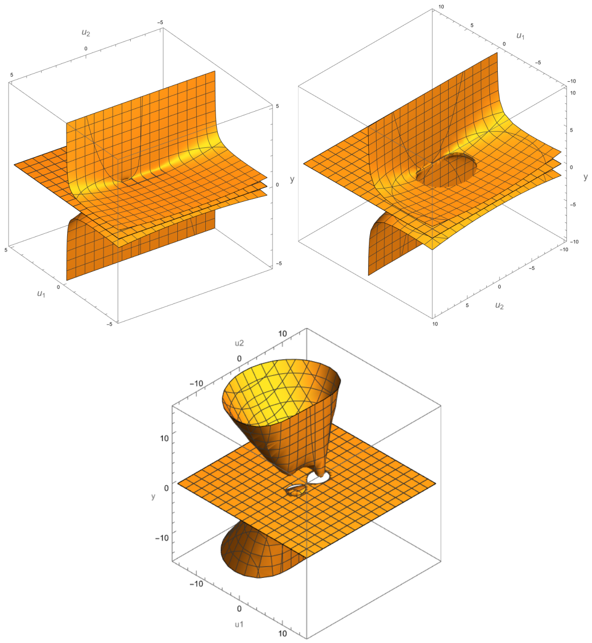
Now, if we specify the necessary parameters ${\mathit{ϵ}}^{\left(\mathit{r}\right)},{\mathit{ϵ}}^{\left(\mathit{i}\right)}$ and ${\mathit{\omega }}_{\mathit{l}}\left(\mathit{\tau }\right)$ included in the algebraic Equation (61), this will allow us to explicitly solve the equation and visualize it as a 2$\mathit{D}$-surface (submanifold ${\mathbf{\Xi }}_{\left\{{\mathbf{u}}^{\left(\mathit{l}\right)}\right\}}^{\left(\mathbf{2}\right)})$. As the calculations performed show (see Figure 1), depending on the set of problem parameters, these submanifolds can possess nontrivial geometric and topological properties. In particular, they can have different Betti numbers, which characterize topological invariants, representing the rank of their, in this case, 2$\mathit{D}$ homology group, and counting the number of 2$\mathit{D}$ “holes”.

5. The Mathematical Expectation of the Wave Function of a Single Photon

5.1. The Measure of the Functional Space

To continue the analytical constructions of the theory, it is necessary to determine the distance between functions in the space ${\mathbf{\Xi }}_{\left\{\mathbf{u}\right(\mathit{\tau }\left)\right\}}$, or more precisely, to determine the measure of the functional space (see [35,37]).

Let the conditional probability $\mathit{P}(\mathbf{u},\mathit{\tau }|{\mathbf{u}}^{\prime },{\mathit{\tau }}^{\prime })$ satisfy the following limiting condition:

$$\begin{array}{c}\hfill \underset{\mathit{\tau }\to {\mathit{\tau }}^{\prime }}{\mathbf{lim}}\mathit{P}(\mathbf{u},\mathit{\tau }|{\mathbf{u}}^{\prime },{\mathit{\tau }}^{\prime })=\mathit{\delta }(\mathbf{u}-{\mathbf{u}}^{\prime }),\mathit{\tau }={\mathit{\tau }}^{\prime }+\mathbf{\Delta }\mathit{\tau }.\end{array}$$

(63)

The latter means that for small intervals, i.e., for $\mathbf{\Delta }\mathit{\tau }=\mathit{\tau }-{\mathit{\tau }}^{\prime }\ll \mathbf{1}$, we can represent the solution of Equations (46) and (47) in the following form:

$$\mathit{P}(\mathbf{u},\mathit{\tau }|{\mathbf{u}}^{\prime },{\mathit{\tau }}^{\prime })={\displaystyle \frac{\mathbf{1}}{\mathbf{2}\mathit{\pi }\sqrt{\left|\mathbf{det}\mathbf{{\rm Y}}\right|}\mathbf{\Delta }\mathit{\tau }}}\mathbf{exp}\left\{-{\displaystyle \frac{{\left[\mathbf{u}-{\mathbf{u}}^{\prime }-\mathbf{K}(\mathbf{u},\mathit{\tau })\mathbf{\Delta }\mathbf{\tau }\right]}^{\mathit{T}}{\mathbf{{\rm Y}}}^{-\mathbf{1}}\left[\mathbf{u}-{\mathbf{u}}^{\prime }-\mathbf{K}(\mathbf{u},\mathit{\tau })\mathbf{\Delta }\mathit{\tau }\right]}{\mathbf{2}\mathbf{\Delta }\mathit{\tau }}}\right\},$$

(64)

where $\mathbf{{\rm Y}}$ is the second-rank matrix with elements; ${\mathit{ϵ}}_{\mathbf{11}}={\mathit{ϵ}}^{\left(\mathit{r}\right)},{\mathit{ϵ}}_{\mathbf{22}}={\mathit{ϵ}}^{\left(\mathit{i}\right)}$ and ${\mathit{ϵ}}_{\mathbf{12}}={\mathit{ϵ}}_{\mathbf{21}}=\mathbf{0}$, while ${[\cdots ]}^{\mathit{T}}$ denotes a vector transposition.

Using (64), we can write an explicit expression for the probability distribution of the transition between two very close points:

$$\begin{array}{c}\hfill \mathit{P}({\mathit{u}}_{\mathbf{1}},{\mathit{u}}_{\mathbf{2}},\mathit{\tau }|{\mathit{u}}_{\mathbf{1}}^{\prime },{\mathit{u}}_{\mathbf{2}}^{\prime },{\mathit{\tau }}^{\prime })={\displaystyle \frac{\mathbf{1}}{\mathbf{2}\mathit{\pi }\sqrt{{\mathit{ϵ}}^{\left(\mathit{r}\right)}{\mathit{ϵ}}^{\left(\mathit{i}\right)}}\mathbf{\Delta }\mathit{\tau }}}\times \\ \hfill \mathbf{exp}\left\{-{\displaystyle \frac{{\left[{\mathit{u}}_{\mathbf{1}}-{\mathit{u}}_{\mathbf{1}}^{\prime }-{\mathit{k}}_{\mathbf{1}}({\mathit{u}}_{\mathbf{1}},{\mathit{u}}_{\mathbf{2}},\mathit{\tau })\mathbf{\Delta }\mathit{\tau }\right]}^{\mathbf{2}}}{\mathbf{2}{\mathit{ϵ}}^{\left(\mathit{r}\right)}\mathbf{\Delta }\mathit{\tau }}}-{\displaystyle \frac{{\left[{\mathit{u}}_{\mathbf{2}}-{\mathit{u}}_{\mathbf{2}}^{\prime }-{\mathit{k}}_{\mathbf{2}}({\mathit{u}}_{\mathbf{1}},{\mathit{u}}_{\mathbf{2}})\mathbf{\Delta }\mathit{\tau }\right]}^{\mathbf{2}}}{\mathbf{2}{\mathit{ϵ}}^{\left(\mathbf{i}\right)}\mathbf{\Delta }\mathit{\tau }}}\right\},\end{array}$$

(65)

where the coefficients ${\mathit{k}}_{\mathbf{1}}$ and ${\mathit{k}}_{\mathbf{2}}$ are defined from Expression (46).

In the case where dissipation in the medium is absent or extremely small, for example, when light passes through a vacuum, it is necessary to set ${\mathit{ϵ}}^{\left(\mathit{i}\right)}=\mathbf{0}$. Accordingly, Distribution (65) takes the following form:

$$\begin{array}{c}\hfill \mathit{P}({\mathit{u}}_{\mathbf{1}},{\mathit{u}}_{\mathbf{2}},\mathit{\tau }|{\mathit{u}}_{\mathbf{1}}^{\prime },{\mathit{u}}_{\mathbf{2}}^{\prime },{\mathit{\tau }}^{\prime })={\displaystyle \frac{\mathbf{1}}{\mathbf{2}\mathit{\pi }\sqrt{{\mathit{ϵ}}^{\left(\mathit{r}\right)}\mathbf{\Delta }\mathit{\tau }}}}\times \\ \hfill \mathbf{exp}\left\{-{\displaystyle \frac{{\left[{\mathit{u}}_{\mathbf{1}}-{\mathit{u}}_{\mathbf{1}}^{\prime }-{\mathit{k}}_{\mathbf{1}}({\mathit{u}}_{\mathbf{1}},{\mathit{u}}_{\mathbf{2}},\mathit{\tau })\mathbf{\Delta }\mathit{\tau }\right]}^{\mathbf{2}}}{\mathbf{2}{\mathit{ϵ}}^{\left(\mathit{r}\right)}\mathbf{\Delta }\mathit{\tau }}}\right\}\mathit{\delta }\left[{\mathit{u}}_{\mathbf{2}}-{\mathit{u}}_{\mathbf{2}}^{\prime }+{\mathit{k}}_{\mathbf{2}}({\mathit{u}}_{\mathbf{1}},{\mathit{u}}_{\mathbf{2}})\right].\end{array}$$

(66)

Finally, taking into account the above, we can write down the probability of transition between any two points along any predetermined trajectory in the functional space ${\mathbf{\Xi }}_{\left\{\mathit{u}\right(\mathit{\tau }\left)\right\}}$:

$$\begin{array}{c}\hfill \mathit{D}\mathit{\mu }\left(\mathbf{u}\right)=\mathit{d}\mathit{\mu }\left({\mathbf{u}}_{\mathbf{0}}\right)\underset{\mathit{N}\to \infty }{\mathbf{lim}}\left\{{\left({\displaystyle \frac{\mathbf{1}}{\mathbf{2}\mathit{\pi }}}{\displaystyle \frac{\mathit{N}/\mathit{\tau }}{\sqrt{{\mathit{ϵ}}^{\left(\mathit{r}\right)}{\mathit{ϵ}}^{\left(\mathit{i}\right)}}}}\right)}^{\mathit{N}}{\displaystyle \prod _{\mathit{l}=\mathbf{0}}^{\mathit{N}}}{\mathit{du}}_{\mathbf{1}(\mathit{l}+\mathbf{1})}{\mathit{du}}_{\mathbf{2}(\mathit{l}+\mathbf{1})}\mathbf{exp}\right[-{\displaystyle \frac{\mathit{N}/\mathit{\tau }}{\mathbf{2}{\mathit{ϵ}}^{\left(\mathit{r}\right)}}}\times \\ \hfill {\left({\mathit{u}}_{\mathbf{1}(\mathit{l}+\mathbf{1})}-{\mathit{u}}_{\mathbf{1}\left(\mathit{l}\right)}-{\mathit{k}}_{\mathbf{1}(\mathit{l}+\mathbf{1})}{\displaystyle \frac{{\mathit{\tau }}_{\mathit{l}+\mathbf{1}}}{\mathit{N}}}\right)}^{\mathbf{2}}-{\displaystyle \frac{\mathit{N}/\mathit{\tau }}{\mathbf{2}{\mathit{ϵ}}^{\left(\mathit{i}\right)}}}{\left({\mathit{u}}_{\mathbf{2}(\mathit{l}+\mathbf{1})}-{\mathit{u}}_{\mathbf{2}\left(\mathit{l}\right)}-{\mathit{k}}_{\mathbf{2}(\mathit{l}+\mathbf{1})}{\displaystyle \frac{{\mathit{\tau }}_{\mathit{l}+\mathbf{1}}}{\mathit{N}}}\right)}^{\mathbf{2}}\left]\right\},\end{array}$$

(67)

where $\mathit{d}\mathit{\mu }\left({\mathbf{u}}_{\mathbf{0}}\right)=\mathit{\delta }({\mathit{u}}_{\mathbf{1}}-{\mathit{u}}_{\mathbf{1}\left(\mathbf{0}\right)})\mathit{\delta }({\mathit{u}}_{\mathbf{2}}-{\mathit{u}}_{\mathbf{2}\left(\mathbf{0}\right)}){\mathit{du}}_{\mathbf{1}}{\mathit{du}}_{\mathbf{2}}$ denotes the measure of the initial distribution; in addition, the following notations are made:

$${\mathit{u}}_{\mathbf{1}\left(\mathit{l}\right)}={\mathit{u}}_{\mathbf{1}}\left({\mathit{\tau }}_{\mathit{l}}\right),{\mathit{u}}_{\mathbf{2}\left(\mathit{l}\right)}={\mathit{u}}_{\mathbf{2}}\left({\mathit{\tau }}_{\mathit{l}}\right),{\mathit{k}}_{\mathbf{1}\left(\mathit{l}\right)}={\mathit{k}}_{\mathbf{1}}({\mathit{u}}_{\mathbf{1}\left(\mathit{l}\right)},{\mathit{u}}_{\mathbf{2}\left(\mathit{l}\right)},{\mathit{\tau }}_{\mathit{l}}),{\mathit{k}}_{\mathbf{2}\left(\mathit{l}\right)}={\mathit{k}}_{\mathbf{2}}({\mathit{u}}_{\mathbf{1}\left(\mathit{l}\right)},{\mathit{u}}_{\mathbf{2}\left(\mathit{l}\right)},{\mathit{\tau }}_{\mathit{l}}).$$

Note that Expression (67) is essentially the Fokker–Planck measure of the functional space ${\mathbf{\Xi }}_{\left\{\mathbf{u}\right(\mathit{\tau }\left)\right\}}$, both in the case when the fluctuation powers are small and when they are large and the corresponding geometry in the limit of statistical equilibrium is non-commutative. Recall that in the limit of statistical equilibrium, the functional space ${\mathbf{\Xi }}_{\left\{\mathbf{u}\right(\mathit{\tau }\left)\right\}}$ is compactified into 4$\mathit{D}$ additional subspace ${\mathbb{R}}_{\left\{\mathbf{u}\right\}}^{\mathbf{4}}$ or ${\mathbf{\Xi }}_{\left\{\mathbf{u}\right\}}^{\left(\mathbf{4}\right)}\left(\mathit{\tau }\right)$, respectively, depending on the values of the fluctuation powers ${\mathit{ϵ}}^{\left(\mathit{r}\right)}$ and ${\mathit{ϵ}}^{\left(\mathit{i}\right)}$.

5.2. The Wave Function of a Single Photon in the Limit of Statistical Equilibrium

Now that we have constructed the Fokker–Planck measure of the functional space (67), in the limit of statistical equilibrium, it is easy to calculate the mathematical expectation of the photon wave function in the plane perpendicular to the direction of photon propagation.

Definition 2. 

The mathematical expectation of a random variable will be determined by the following integral over the functional space ${\mathbf{\Xi }}_{\left\{\mathit{u}\right(\mathit{\tau }\left)\right\}}$:

$$\mathbb{E}\left[\mathcal{G}({\mathit{q}}_{\mathbf{1}},{\mathit{q}}_{\mathbf{2}},\mathit{\tau };\left\{\mathit{f}\right\})\right]={\int }_{{\mathbf{\Xi }}_{\left\{\mathit{u}\right(\mathit{\tau }\left)\right\}}}\mathcal{G}({\mathit{q}}_{\mathbf{1}},{\mathit{q}}_{\mathbf{2}},\mathit{\tau };\left\{\mathit{f}\right\})\mathit{D}\mathit{\mu }\left(\mathit{u}\right).$$

(68)

where $\mathcal{G}({\mathit{q}}_{\mathbf{1}},{\mathit{q}}_{\mathbf{2}},\mathit{\tau };\left\{\mathit{f}\right\})$ is a random variable, and $\mathbb{E}\left[\cdots \right]$ denotes the mathematical expectation.

The solution of the Langevin–Schrödinger Equation (35) for a photon moving in a nanowaveguide with random influences can be represented as follows:

$$\mathcal{F}\left(\mathbf{n}\right|\mathbf{q},\mathit{\tau };\left\{\mathit{f}\right\})={\displaystyle \prod _{\mathit{l}=\mathbf{1}}^{\mathbf{2}}}{\mathcal{F}}_{\mathit{l}}\left({\mathit{n}}_{\mathit{l}}\right|{\mathit{q}}_{\mathit{l}},\mathit{\tau };\left\{{\mathit{f}}_{\mathit{l}}\right\}).$$

(69)

Taking into account (68) and the fact that the additional subspace in general is reduced to the direct product of two 2$\mathit{D}$ subspaces (see Section 4.2 and Section 4.3), it is easy to prove that the mathematical expectation of the photon wave function can be written in factorized form:

$$\mathbb{E}\left[\mathcal{F}\left(\mathbf{n}\right|\mathbf{q},\mathit{\tau };\left\{\mathit{f}\right\})\right]={\displaystyle \prod _{\mathit{l}=\mathbf{1}}^{\mathbf{2}}}\mathbb{E}\left[{\mathcal{F}}_{\mathit{l}}\left({\mathit{n}}_{\mathit{l}}\right|{\mathit{q}}_{\mathit{l}},\mathit{\tau };\left\{{\mathit{f}}_{\mathit{l}}\right\})\right],$$

(70)

where

$$\mathbb{E}\left[{\mathcal{F}}_{\mathit{l}}\left({\mathit{n}}_{\mathit{l}}\right|{\mathit{q}}_{\mathit{l}},\mathit{\tau };\left\{{\mathit{f}}_{\mathit{l}}\right\})\right]={\int }_{{\mathbf{\Xi }}_{\left\{{\mathbf{u}}^{\left(\mathit{l}\right)}\left(\mathit{\tau }\right)\right\}}}{\mathcal{F}}_{\mathit{l}}\left({\mathit{n}}_{\mathit{l}}\right|{\mathit{q}}_{\mathit{l}},\mathit{\tau };\left\{{\mathit{f}}_{\mathit{l}}\right\})\mathit{D}\mathit{\mu }\left({\mathbf{u}}^{\left(\mathit{l}\right)}\right).$$

(71)

Before we start calculating the functional integral (71), it is important to write down the explicit form of the photon random wave function for an arbitrary quantum state. In particular, taking into account (42) and (44), we can write:

$${\mathcal{F}}_{\mathit{l}}\left({\mathit{n}}_{\mathit{l}}\right|{\mathit{q}}_{\mathit{l}},\mathit{\tau };\left\{{\mathit{f}}_{\mathit{l}}\right\})=\sqrt{{\displaystyle \frac{\mathbf{1}}{{\mathbf{2}}^{{\mathit{n}}_{\mathit{l}}}{\mathit{n}}_{\mathit{l}}!\sqrt{\mathit{\pi }}}}}\mathbf{exp}\left\{{\displaystyle \frac{\mathbf{1}}{\mathbf{2}}}\left[\mathit{i}{\mathbf{\Pi }}^{\prime }\left(\mathit{\tau }\right){\mathit{q}}_{\mathit{l}}^{\mathbf{2}}-\mathbf{\Pi }\left(\mathit{\tau }\right)\right]\right\}{\mathit{H}}_{{\mathit{n}}_{\mathit{l}}}\left({\mathit{q}}_{\mathit{l}}{\mathit{e}}^{-{\mathit{n}}_{\mathit{l}}\mathbf{\Pi }\left(\mathit{\tau }\right)}\right).$$

(72)

where ${\mathbf{\Pi }}_{\mathit{l}}\left(\mathit{\tau }\right)={\int }_{\mathbf{0}}^{\mathit{\tau }}\left[{\mathit{u}}_{\mathbf{1}}^{\left(\mathit{l}\right)}\left({\mathit{\tau }}^{\prime }\right)+{\mathit{iu}}_{\mathbf{2}}^{\left(\mathit{l}\right)}\left({\mathit{\tau }}^{\prime }\right)\right]\mathit{d}{\mathit{\tau }}^{\prime }$ (see (42), definition of the function $\mathbf{\Pi }\left(\mathit{\tau }\right)$), in addition, ${\mathbf{\Pi }}^{\prime }\left(\mathit{\tau }\right)=\mathit{d}\mathbf{\Pi }\left(\mathit{\tau }\right)/\mathit{d}\mathit{\tau }$. Below, to simplify notation, the index “$\mathit{l}$” above the variables ${\mathit{u}}_{\mathbf{1}}$ and ${\mathit{u}}_{\mathbf{2}}$ will be omitted.

From Expression (72), it is easy to find the wave functions of the first two quantum states:

$$\begin{array}{c}\hfill {\mathcal{F}}_{\mathit{l}}\left(\mathbf{0}\right|{\mathit{q}}_{\mathit{l}},\mathit{\tau };\left\{{\mathit{f}}_{\mathit{l}}\right\})=\sqrt{{\displaystyle \frac{\mathbf{1}}{\sqrt{\mathit{\pi }}}}}\mathbf{exp}\left\{-{\displaystyle \frac{\mathbf{1}}{\mathbf{2}}}{\displaystyle \underset{\mathbf{0}}{\overset{\mathit{\tau }}{\int }}}\right({\mathit{u}}_{\mathbf{1}}\left({\mathit{\tau }}^{\prime }\right)+{\mathit{iu}}_{\mathbf{2}}\left({\mathit{\tau }}^{\prime }\right))\mathit{d}{\mathit{\tau }}^{\prime }+{\displaystyle \frac{\mathbf{1}}{\mathbf{2}}}({\mathit{iu}}_{\mathbf{1}}-{\mathit{u}}_{\mathbf{2}}){\mathit{q}}_{\mathit{l}}^{\mathbf{2}}\},\\ \hfill {\mathcal{F}}_{\mathit{l}}\left(\mathbf{1}\right|{\mathit{q}}_{\mathit{l}},\mathit{\tau };\left\{{\mathit{f}}_{\mathit{l}}\right\})={\mathit{q}}_{\mathit{l}}\sqrt{{\displaystyle \frac{\mathbf{1}}{\mathbf{2}\sqrt{\mathit{\pi }}}}}\mathbf{exp}\left\{-{\displaystyle \frac{\mathbf{3}}{\mathbf{2}}}{\displaystyle \underset{\mathbf{0}}{\overset{\mathit{\tau }}{\int }}}\left({\mathit{u}}_{\mathbf{1}}\left({\mathit{\tau }}^{\prime }\right)+{\mathit{iu}}_{\mathbf{2}}\left({\mathit{\tau }}^{\prime }\right)\right)\mathit{d}{\mathit{\tau }}^{\prime }+{\displaystyle \frac{\mathbf{1}}{\mathbf{2}}}({\mathit{iu}}_{\mathbf{1}}-{\mathit{u}}_{\mathbf{2}}){\mathit{q}}_{\mathit{l}}^{\mathbf{2}}\right\}.\end{array}$$

(73)

Substituting (73) into (71) and using the generalized Feynman–Kac theorem [39], we can calculate the corresponding functional integrals and find the ME of the photon wave function in various quantum states, representing them as double integrals:

$$\begin{array}{c}\hfill {\overline{\mathcal{F}}}_{\mathit{l}}\left(\mathbf{0}\right|{\mathit{q}}_{\mathit{l}},\mathit{\tau };\left\{{\mathit{f}}_{\mathit{l}}\right\})=\sqrt{{\displaystyle \frac{\mathbf{1}}{\sqrt{\mathit{\pi }}}}}{\displaystyle \underset{-\infty }{\overset{+\infty }{\int }}}{\mathit{du}}_{\mathit{1}}{\displaystyle \underset{\mathbf{0}}{\overset{+\infty }{\int }}}{\mathit{du}}_{\mathbf{2}}{\mathit{Q}}_{\mathit{l}}(\mathbf{0};{\mathit{u}}_{\mathbf{1}},{\mathit{u}}_{\mathbf{2}},\mathit{\tau }){\mathit{e}}^{{\mathcal{A}}_{\mathit{l}}({\mathit{u}}_{\mathbf{1}},{\mathit{u}}_{\mathbf{2}};{\mathit{q}}_{\mathit{l}})},\\ \hfill {\overline{\mathcal{F}}}_{\mathit{l}}\left(\mathbf{1}\right|{\mathit{q}}_{\mathit{l}},\mathit{\tau };\left\{{\mathit{f}}_{\mathit{l}}\right\})={\mathit{q}}_{\mathit{l}}\sqrt{{\displaystyle \frac{\mathbf{1}}{\mathbf{2}\sqrt{\mathit{\pi }}}}}{\displaystyle \underset{-\infty }{\overset{+\infty }{\int }}}{\mathit{du}}_{\mathit{1}}{\displaystyle \underset{\mathbf{0}}{\overset{+\infty }{\int }}}{\mathit{du}}_{\mathbf{2}}{\mathit{Q}}_{\mathit{l}}(\mathbf{1};{\mathit{u}}_{\mathbf{1}},{\mathit{u}}_{\mathbf{2}},\mathit{\tau }){\mathit{e}}^{{\mathcal{A}}_{\mathit{l}}({\mathit{u}}_{\mathbf{1}},{\mathit{u}}_{\mathbf{2}};{\mathit{q}}_{\mathit{l}})},\end{array}$$

(74)

where ${\mathcal{A}}_{\mathit{l}}({\mathit{u}}_{\mathbf{1}},{\mathit{u}}_{\mathbf{2}};{\mathit{q}}_{\mathit{l}})=({\mathit{iu}}_{\mathbf{1}}-{\mathit{u}}_{\mathbf{2}}){\mathit{q}}_{\mathit{l}}^{\mathbf{2}}/\mathbf{2}$ and ${\overline{\mathcal{F}}}_{\mathit{l}}\left(\mathit{n}\right|{\mathit{q}}_{\mathit{l}},\mathit{\tau };\left\{{\mathit{f}}_{\mathit{l}}\right\})=\mathbb{E}\left[{\mathcal{F}}_{\mathit{l}}\left(\mathit{n}\right|{\mathit{q}}_{\mathit{l}},\mathit{\tau };\left\{{\mathit{f}}_{\mathit{l}}\right\})\right]$ denotes the ME of the wave function.

As for the integrand ${\mathit{Q}}_{\mathit{l}}(\mathit{n};{\mathit{u}}_{\mathbf{1}},{\mathit{u}}_{\mathbf{2}},\mathit{\tau })$, it is a solution to the following second-order complex PDE:

$${\partial }_{\mathit{\tau }}{\mathit{Q}}_{\mathit{l}}(\mathit{n};{\mathit{u}}_{\mathbf{1}},{\mathit{u}}_{\mathbf{2}},\mathit{\tau })=\left\{{\widehat{\mathit{L}}}_{\mathit{l}}-(\mathit{n}+\mathbf{1}/\mathbf{2})({\mathit{u}}_{\mathbf{1}}+{\mathit{iu}}_{\mathbf{2}})\right\}{\mathit{Q}}_{\mathit{l}}(\mathit{n};{\mathit{u}}_{\mathbf{1}},{\mathit{u}}_{\mathbf{2}},\mathit{\tau }),\mathit{n}=\mathbf{0},\mathbf{1},\mathbf{2},\dots ,$$

(75)

where the operator ${\widehat{\mathit{L}}}_{\mathit{l}}$ is defined by Formula (47).

By representing the solution of Equation (75) as a sum:

$${\mathit{Q}}_{\mathit{l}}(\mathit{n};{\mathit{u}}_{\mathbf{1}},{\mathit{u}}_{\mathbf{2}},\mathit{\tau })={\mathit{Q}}_{\mathit{l}}^{\left(\mathit{r}\right)}(\mathit{n};{\mathit{u}}_{\mathbf{1}},{\mathit{u}}_{\mathbf{2}},\mathit{\tau })+{\mathit{iQ}}_{\mathit{l}}^{\left(\mathit{i}\right)}(\mathit{n};{\mathit{u}}_{\mathbf{1}},{\mathit{u}}_{\mathbf{2}},\mathit{\tau }),$$

(76)

we can obtain the following system of PDEs:

$$\{\begin{array}{c}{\partial }_{\mathit{\tau }}{\mathit{Q}}_{\mathit{l}}^{\left(\mathit{r}\right)}=\left\{{\widehat{\mathit{L}}}_{\mathit{l}}-(\mathit{n}+\mathbf{1}/\mathbf{2}){\mathit{u}}_{\mathbf{1}}\right\}{\mathit{Q}}_{\mathit{l}}^{\left(\mathit{r}\right)}+(\mathit{n}+\mathbf{1}/\mathbf{2}){\mathit{u}}_{\mathbf{2}}{\mathit{Q}}_{\mathit{l}}^{\left(\mathit{i}\right)},\hfill \\ {\partial }_{\mathit{\tau }}{\mathit{Q}}_{\mathit{l}}^{\left(\mathit{i}\right)}=\left\{{\widehat{\mathit{L}}}_{\mathit{l}}-(\mathit{n}+\mathbf{1}/\mathbf{2}){\mathit{u}}_{\mathbf{1}}\right\}{\mathit{Q}}_{\mathit{l}}^{\left(\mathit{i}\right)}-(\mathit{n}+\mathbf{1}/\mathbf{2}){\mathit{u}}_{\mathbf{2}}{\mathit{Q}}_{\mathit{l}}^{\left(\mathit{r}\right)}.\hfill \end{array}$$

(77)

The functions ${\mathit{Q}}_{\mathit{l}}^{\left(\mathit{r}\right)}$ and ${\mathit{Q}}_{\mathit{l}}^{\left(\mathit{i}\right)}$ can be given a probabilistic meaning and normalized to unity. In particular, in what follows we will use the normalized distributions ${\overline{\mathit{Q}}}_{\mathit{l}}^{\left(\mathit{r}\right)}$ and ${\overline{\mathit{Q}}}_{\mathit{l}}^{\left(\mathit{i}\right)}$, which are defined by the following expressions:

$$\begin{array}{c}\hfill {\overline{\mathit{Q}}}_{\mathit{l}}^{\left(\mathit{\upsilon }\right)}(\mathit{n};{\mathit{u}}_{\mathbf{1}},{\mathit{u}}_{\mathbf{2}},\mathit{\tau })={\mathit{Q}}_{\mathit{l}}^{\left(\mathit{\upsilon }\right)}(\mathit{n};{\mathit{u}}_{\mathbf{1}},{\mathit{u}}_{\mathbf{2}},\mathit{\tau })/{\mathit{J}}_{\mathit{l}}(\mathit{n};\mathit{\tau }),\mathit{\upsilon }=\mathit{i},\mathit{r},\end{array}$$

(78)

where ${\mathit{J}}_{\mathit{l}}(\mathit{n};\mathit{\tau })$ is the probability normalization coefficient, determined by the following expression:

$${\mathit{J}}_{\mathit{l}}(\mathit{n};\mathit{\tau })={\int }_{\mathbf{0}}^{+\infty }{\int }_{-\infty }^{+\infty }\left[{\mathit{Q}}_{\mathit{l}}^{\left(\mathit{r}\right)}(\mathit{n};{\mathit{u}}_{\mathit{1}},{\mathit{u}}_{\mathit{2}},\mathit{\tau })+{\mathit{Q}}_{\mathit{l}}^{\left(\mathit{i}\right)}(\mathit{n};{\mathit{u}}_{\mathbf{1}},{\mathit{u}}_{\mathbf{2}},\mathit{\tau })\right]{\mathit{du}}_{\mathbf{1}}{\mathit{du}}_{\mathbf{2}}.$$

It is obvious that after normalization of the distributions ${\overline{\mathit{Q}}}_{\mathit{l}}^{\left(\mathit{r}\right)}({\mathit{u}}_{\mathbf{1}},{\mathit{u}}_{\mathbf{2}},\mathit{\tau })$ and ${\overline{\mathit{Q}}}_{\mathit{l}}^{\left(\mathit{i}\right)}({\mathit{u}}_{\mathbf{1}},{\mathit{u}}_{\mathbf{2}},\mathit{\tau })$, the probability in JS is preserved and, accordingly, the equality is satisfied:

$${\int }_{\mathbf{0}}^{+\infty }{\int }_{-\infty }^{+\infty }\left[{\overline{\mathit{Q}}}_{\mathit{l}}^{\left(\mathit{r}\right)}(\mathit{n};{\mathit{u}}_{\mathit{1}},{\mathit{u}}_{\mathbf{2}},\mathit{\tau })+{\overline{\mathit{Q}}}_{\mathit{l}}^{\left(\mathit{i}\right)}(\mathit{n};{\mathit{u}}_{\mathbf{1}},{\mathit{u}}_{\mathbf{2}},\mathit{\tau })\right]{\mathit{du}}_{\mathbf{1}}{\mathit{du}}_{\mathbf{2}}=\mathbf{1}.$$

(79)

Now, returning to the ME of wave function (74), it is necessary to note that it, in essence, describes a “closed”, self-consistent, JS “photon + environment” and therefore must be normalized to unity. In other words, the normalized ME of the photon’s wave function will be represented as follows:

$${\underline{\overline{\mathcal{F}}}}_{\mathit{l}}\left(\mathit{n}\right|{\mathit{q}}_{\mathit{l}},\mathit{\tau };\left\{{\mathit{f}}_{\mathit{l}}\right\})={\overline{\mathcal{F}}}_{\mathit{l}}\left(\mathit{n}\right|{\mathit{q}}_{\mathit{l}},\mathit{\tau };\left\{{\mathit{f}}_{\mathit{l}}\right\})/{\mathcal{J}}_{\mathit{l}}(\mathit{n},\mathit{\tau }),$$

(80)

where ${\mathcal{J}}_{\mathit{l}}(\mathit{n},\mathit{\tau })={\int }_{-\infty }^{+\infty }{\overline{\mathcal{F}}}_{\mathit{l}}\left(\mathit{n}\right|{\mathit{q}}_{\mathit{l}},\mathit{\tau };\left\{{\mathit{f}}_{\mathit{l}}\right\}){\overline{\mathcal{F}}}_{\mathit{l}}^{*}\left(\mathit{n}\right|{\mathit{q}}_{\mathit{l}},\mathit{\tau };\left\{{\mathit{f}}_{\mathit{l}}\right\}){\mathit{dq}}_{\mathit{l}}$ is the normalization factor.

To solve the SDEs system, it is convenient to formulate the Neumann initial-boundary value problem. In particular, we will represent the initial distributions as the product of two Dirac delta-functions over the perpendicular coordinates ${\mathit{u}}_{\mathbf{1}}$ and ${\mathit{u}}_{\mathbf{2}}$, accordingly:

$${\overline{\mathit{Q}}}_{\mathit{l}}^{\left(\mathit{\upsilon }\right)}(\mathit{n};{\mathit{u}}_{\mathbf{1}},{\mathit{u}}_{\mathbf{2}},\mathit{\tau }){|}_{\mathit{\tau }=\mathbf{0}}={\displaystyle \prod _{\mathit{j}=\mathbf{1}}^{\mathbf{2}}}\mathit{\delta }({\mathit{u}}_{\mathit{j}}-{\mathit{u}}_{\mathbf{0}\mathit{j}}),\mathit{\upsilon }=\mathit{i},\mathit{r}.$$

(81)

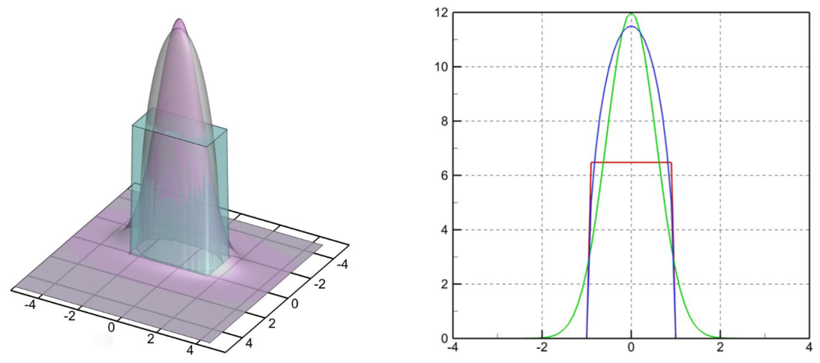
Recall that the product of two Dirac delta-functions should be understood in such a way that when ${\mathit{u}}_{\mathbf{1}}={\mathit{u}}_{\mathbf{01}}$ and ${\mathit{u}}_{\mathbf{2}}={\mathit{u}}_{\mathbf{02}}$, it is infinite, and in all other cases, it is zero. Nevertheless, in a specific numerical solution of the problem, instead of Dirac delta functions, we use Gaussian functions, see Section 8 and Figure 2.

Based on the conditions of the problem under consideration, we can write the normalization condition for the total probability as follows:

$${\int }_{\mathbf{0}}^{+\infty }{\int }_{-\infty }^{+\infty }\left[\mathit{p}{\overline{\mathit{Q}}}_{\mathit{l}}^{\left(\mathit{r}\right)}(\mathit{n};{\mathit{u}}_{\mathbf{1}},{\mathit{u}}_{\mathbf{2}},{\mathit{\tau }}_{\mathbf{0}})+(\mathbf{1}-\mathit{p}){\overline{\mathit{Q}}}_{\mathit{l}}^{\left(\mathit{i}\right)}(\mathit{n};{\mathit{u}}_{\mathbf{1}},{\mathit{u}}_{\mathbf{2}},{\mathit{\tau }}_{\mathbf{0}})\right]{\mathit{du}}_{\mathbf{1}}{\mathit{du}}_{\mathbf{2}}=\mathbf{1}/\mathbf{2},$$

(82)

where $\mathit{p}\in [\mathbf{0},\mathbf{1}]$ denotes the weight of the distribution associated with elastic quantum processes accompanying a photon in the environment, and $(\mathbf{1}-\mathit{p})$ is the weight of the distribution associated with inelastic quantum processes. Thus, the probability distributions ${\overline{\mathit{Q}}}_{\mathit{l}}^{\left(\mathit{r}\right)}(\mathit{n};{\mathit{u}}_{\mathbf{1}},{\mathit{u}}_{\mathbf{2}},\mathit{\tau })$ and ${\overline{\mathit{Q}}}_{\mathit{l}}^{\left(\mathit{i}\right)}(\mathit{n};{\mathit{u}}_{\mathbf{1}},{\mathit{u}}_{\mathbf{2}},\mathit{\tau })$ are combined into a common probability, starting from the initial moment of evolution time ${\mathit{tau}}_{\mathbf{0}}$ for a single photon. If we check the probability normalization condition (82) for the initial time $\mathit{\tau }=\mathbf{0}$, then it is easy to verify that the initial distributions (81) satisfy the normalization to unity, since the integration over the coordinate ${\mathit{u}}_{\mathbf{2}}$ is carried out over the segment of the numerical axis $[\mathbf{0},\infty )$, i.e., ${\int }_{\mathbf{0}}^{\infty }\mathit{\delta }\left({\mathit{u}}_{\mathbf{2}}\right){\mathit{du}}_{\mathbf{2}}=\mathbf{1}/\mathbf{2}.$

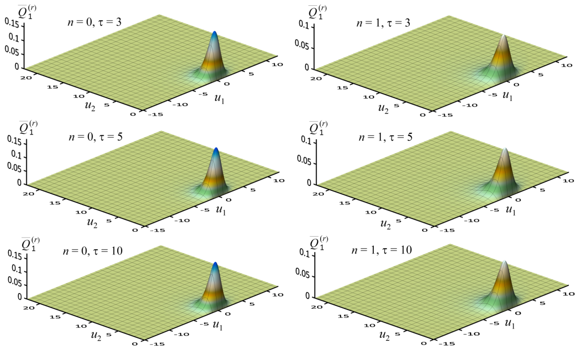
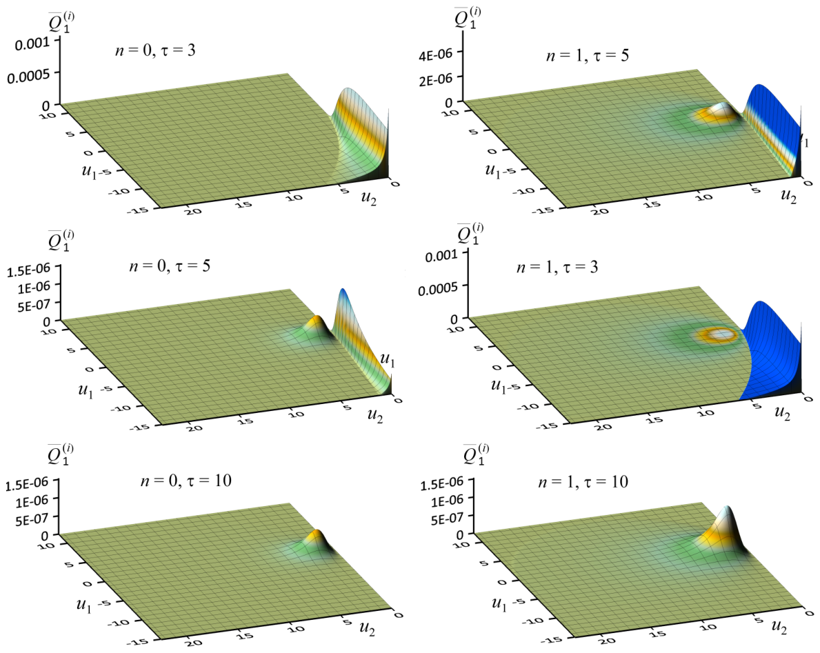
Below are visualizations (see graphs in Figure 3 and Figure 4) of calculations of the evolution of normalized distributions of the environmental fields ${\overline{\mathit{Q}}}_{\mathbf{1}}^{\left(\mathit{r}\right)}$ and ${\overline{\mathit{Q}}}_{\mathbf{1}}^{\left(\mathit{i}\right)}$ in the ground and first excited states. As can be seen from the graphs, in the process of evolution of QS under certain conditions of the problem, a fairly rapid transfer of probability occurs from the distribution ${\overline{\mathit{Q}}}_{\mathbf{1}}^{\left(\mathit{i}\right)}$ to ${\overline{\mathit{Q}}}_{\mathbf{1}}^{\left(\mathit{r}\right)}$.

As for the boundary conditions for solving the system of partial differential Equation (77), they should be specified on the axis ${\mathit{u}}_{\mathbf{1}}$, the natural boundary of the problem, as follows:

$${\displaystyle \frac{\partial {\overline{\mathit{Q}}}_{\mathit{l}}^{\left(\mathit{\upsilon }\right)}(\mathit{n};{\mathit{u}}_{\mathbf{1}},{\mathit{u}}_{\mathbf{2}},\mathit{\tau })}{\partial {\mathit{u}}_{\mathbf{2}}}}{|}_{{\mathit{u}}_{\mathbf{2}}=\mathbf{0}}={\overline{\mathit{Q}}}_{\mathit{l}}^{\left(\mathit{\upsilon }\right)}(\mathit{n};{\mathit{u}}_{\mathbf{1}},\mathbf{0},\mathit{\tau })={\mathbb{Q}}_{\mathit{l}}^{\left(\mathit{\upsilon }\right)}(\mathit{n};{\mathit{u}}_{\mathbf{1}},\mathit{\tau }).$$

(83)

Finally, using Expressions (70) and (74), we can construct the mathematical expectations of the first four quantum states of a photon in a nanowaveguide:

$$\begin{array}{c}\hfill \mathbb{E}\left[\mathcal{F}(\mathbf{0},\mathbf{0}|\mathbf{q},\mathit{\tau };\left\{\mathit{f}\right\})\right]={\overline{\mathcal{F}}}_{\mathbf{1}}\left(\mathbf{0}\right|{\mathit{q}}_{\mathbf{1}},\mathit{\tau };\left\{{\mathit{f}}_{\mathbf{1}}\right\})·{\overline{\mathcal{F}}}_{\mathbf{2}}\left(\mathbf{0}\right|{\mathit{q}}_{\mathbf{2}},\mathit{\tau };\left\{{\mathit{f}}_{\mathbf{2}}\right\}),\\ \hfill \mathbb{E}\left[\mathcal{F}(\mathbf{0},\mathbf{1}|\mathbf{q},\mathit{\tau };\left\{\mathit{f}\right\})\right]={\overline{\mathcal{F}}}_{\mathbf{1}}\left(\mathbf{0}\right|{\mathit{q}}_{\mathit{l}},\mathit{\tau };\left\{{\mathit{f}}_{\mathbf{1}}\right\})·{\overline{\mathcal{F}}}_{\mathbf{2}}\left(\mathbf{1}\right|{\mathit{q}}_{\mathbf{2}},\mathit{\tau };\left\{{\mathit{f}}_{\mathbf{2}}\right\}),\\ \hfill \mathbb{E}\left[\mathcal{F}(\mathbf{1},\mathbf{0}|\mathbf{q},\mathit{\tau };\left\{\mathit{f}\right\})\right]={\overline{\mathcal{F}}}_{\mathbf{1}}\left(\mathbf{1}\right|{\mathit{q}}_{\mathbf{1}},\mathit{\tau };\left\{{\mathit{f}}_{\mathbf{1}}\right\})·{\overline{\mathcal{F}}}_{\mathbf{2}}\left(\mathbf{0}\right|{\mathit{q}}_{\mathbf{2}},\mathit{\tau };\left\{{\mathit{f}}_{\mathbf{2}}\right\}),\\ \hfill \mathbb{E}\left[\mathcal{F}(\mathbf{1},\mathbf{1}|\mathbf{q},\mathit{\tau };\left\{\mathbf{f}\right\})\right]={\overline{\mathcal{F}}}_{\mathbf{1}}\left(\mathbf{1}\right|{\mathit{q}}_{\mathbf{1}},\mathbf{\tau };\left\{{\mathit{f}}_{\mathbf{1}}\right\})·{\overline{\mathcal{F}}}_{\mathbf{2}}\left(\mathbf{1}\right|{\mathit{q}}_{\mathbf{2}},\mathit{\tau };\left\{{\mathit{f}}_{\mathbf{2}}\right\}).\end{array}$$

(84)

Recall that the quantum states of the photon $\mathbb{E}\left[\mathcal{F}(\mathbf{0},\mathbf{1}|\mathbf{q},\mathit{\tau };\left\{\mathit{f}\right\})\right]$ and $\mathbb{E}\left[\mathcal{F}(\mathbf{1},\mathbf{0}|\mathbf{q},\mathit{\tau };\left\{\mathit{f}\right\})\right]$ are, in the general case, obviously different and do not coincide.

Based on the obtained formulas for the mathematical expectation of the wave function of a photon in various quantum states (84), one can write the corresponding distributions of the photon energy density in 3$\mathit{D}$ space as a function of time:

$$\begin{array}{c}\hfill {\mathcal{W}}_{\mathit{nm}}={\left|\mathbb{E}\left[\mathcal{F}(\mathit{n},\mathit{m}|\mathbf{q},\mathit{\tau };\left\{\mathit{f}\right\})\right]\right|}^{\mathbf{2}}={\left|{\overline{\mathcal{F}}}_{\mathbf{1}}\left(\mathit{n}\right|{\mathit{q}}_{\mathbf{1}},\mathit{\tau };\left\{{\mathit{f}}_{\mathbf{1}}\right\})\right|}^{\mathbf{2}}·{\left|{\overline{\mathcal{F}}}_{\mathbf{2}}\left(\mathit{m}\right|{\mathit{q}}_{\mathbf{2}},\mathit{\tau };\left\{{\mathit{f}}_{\mathbf{2}}\right\})\right|}^{\mathbf{2}},\end{array}$$

(85)

where $\mathit{n}$ and $\mathit{m}$ are vibrational quantum numbers. In order for ${\mathcal{W}}_{\mathit{nm}}$ to acquire the meaning of the probability distribution of the energy of electromagnetic fields in a single photon, it is necessary to replace the wave functions in the expressions (85) on normalized functions (80).

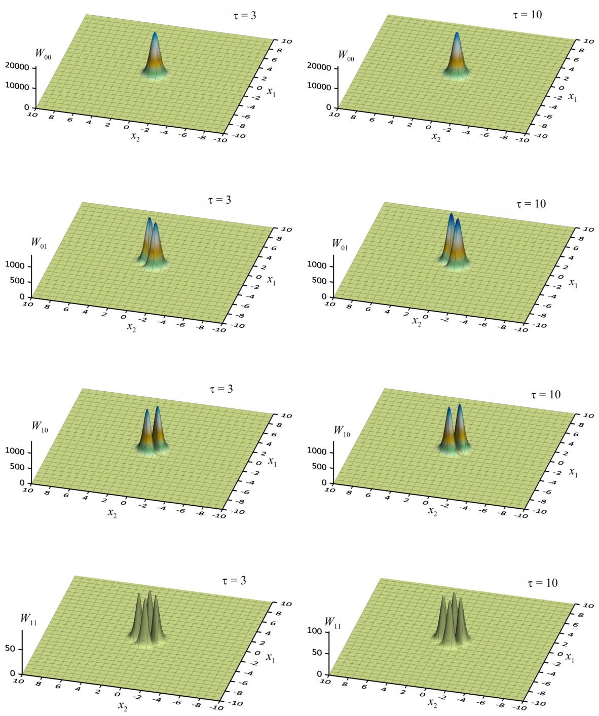
Below, in Section 9.2, for one particular set of initial data, see

Table 1. Parameters of classical oscillators.

	${\mathit{a}}_1$	${\mathit{a}}_2$	${\mathit{b}}_1$	${\mathit{b}}_2$	${\mathit{\gamma }}_1$	${\mathit{\gamma }}_2$	${\mathit{\nu }}_1$	${\mathit{\nu }}_2$
${\mathit{\omega }}_{\mathbf{1}}\left(\mathit{\tau }\right)\to$	{2	-	2	-	2	-	3	-}
${\mathit{\omega }}_{\mathbf{2}}\left(\mathit{\tau }\right)\to$	{-	2	-	2	-	4	-	5}

, the spatial distribution of the electromagnetic fields energy of one photon for the first four quantum states is calculated and visualized, see Figure 5.

5.3. Reduced Density Matrix: Quantized Small Environment

Now, it is important to construct the elements of the reduced density matrix, which play an important role in calculating various QS parameters. Taking into account (72), we can write the following expression for the element of the stochastic density matrix:

$${\mathit{\rho }}_{\mathit{nm}}(\mathbf{q},\mathit{\tau };\left\{\mathit{f}\right\}:{\mathbf{q}}^{\prime },{\mathit{\tau }}^{\prime };\left\{{\mathit{f}}^{\prime }\right\})=\mathcal{F}(\mathit{n},\mathit{m}|\mathbf{q},\mathit{\tau };\left\{\mathit{f}\right\})·{\mathcal{F}}^{*}(\mathit{n},\mathit{m}|{\mathbf{q}}^{\prime },{\mathit{\tau }}^{\prime };\left\{{\mathit{f}}^{\prime }\right\}).$$

Definition 3. 

An element of the reduced density matrix (RDM) ${\mathit{\rho }}_{\mathit{nm}}(\mathit{q},\mathit{\tau })$ will be called the mathematical expectation of an element of a random density matrix ${\mathit{\rho }}_{\mathit{nm}}(\mathit{q},\mathit{\tau };\left\{\mathit{f}\right\}:{\mathit{q}}^{\prime },{\mathit{\tau }}^{\prime };{\left\{\mathit{f}\right\}}^{\prime })$, obtained after functional integration:

$${\mathit{\rho }}_{\mathit{nm}}(\mathit{q},\mathit{\tau })={\mathit{Tr}}_{\left\{\mathit{u}\right(\mathit{\tau }\left)\right\}}\left[{\mathit{\rho }}_{\mathit{nm}}(\mathit{q},\mathit{\tau };\left\{\mathit{f}\right\}:{\mathit{q}}^{\prime },{\mathit{\tau }}^{\prime };\left\{{\mathit{f}}^{\prime }\right\})\right]{|}_{\mathit{q}={\mathit{q}}^{\prime };\mathit{\tau }={\mathit{\tau }}^{\prime }},$$

(86)

where the operation ${\mathit{Tr}}_{\left\{\mathit{u}\right(\mathit{\tau }\left)\right\}}$ denotes the functional integration over the environment fields:

$$\begin{array}{c}\hfill {\mathit{Tr}}_{\left\{\mathit{u}\right(\mathit{\tau }\left)\right\}}\left[\mathit{\rho }(\mathit{q},\mathit{\tau };\left\{\mathit{f}\right\}:{\mathit{q}}^{\prime },{\mathit{\tau }}^{\prime };\left\{{\mathit{f}}^{\prime }\right\})\right]={\int }_{{\mathbf{\Xi }}_{\left\{\mathit{u}\right(\mathit{\tau }\left)\right\}}}\mathit{\rho }(\mathit{q},\mathit{\tau };\left\{\mathit{f}\right\}|{\mathit{q}}^{\prime },{\mathit{\tau }}^{\prime };\left\{{\mathit{f}}^{\prime }\right\})\mathit{D}\left\{\mathit{u}\left(\mathit{\tau }\right)\right\}.\end{array}$$

(87)

By substituting the corresponding random wave function from (72) into Expression (86) and (87) and performing functional integration, one can find the corresponding element of the RDM. In particular, after simple calculations for the first four elements of the RMD, the following expressions can easily be found:

$$\begin{array}{c}\hfill {\mathit{\varrho }}_{\mathbf{00}}(\mathbf{q},\mathit{\tau })={\displaystyle \prod _{\mathit{l}=\mathbf{1}}^{\mathbf{2}}}{\mathit{\varrho }}_{\mathbf{0}}^{\left(\mathit{l}\right)}={\displaystyle \frac{\mathbf{1}}{\mathit{\pi }}}{\displaystyle \prod _{\mathit{l}=\mathbf{1}}^{\mathbf{2}}}{\int }_{-\infty }^{+\infty }{\mathit{du}}_{\mathbf{1}}{\int }_{\mathbf{0}}^{+\infty }{\mathit{du}}_{\mathbf{2}}{\mathcal{P}}_{\mathit{l}}(\mathbf{0};{\mathit{u}}_{\mathbf{1}},{\mathit{u}}_{\mathbf{2}},\mathit{\tau }){\mathit{e}}^{-{\mathit{u}}_{\mathbf{2}}{\mathit{q}}_{\mathit{l}}^{\mathbf{2}}},\\ \hfill {\mathit{\varrho }}_{\mathbf{11}}(\mathbf{q},\mathit{\tau })={\displaystyle \prod _{\mathit{l}=\mathbf{1}}^{\mathbf{2}}}{\mathit{\varrho }}_{\mathbf{1}}^{\left(\mathit{l}\right)}={\displaystyle \frac{{\mathit{q}}_{\mathbf{1}}^{\mathbf{2}}{\mathit{q}}_{\mathbf{2}}^{\mathbf{2}}}{\mathbf{4}\mathit{\pi }}}{\displaystyle \prod _{\mathit{l}=\mathbf{1}}^{\mathbf{2}}}{\int }_{-\infty }^{+\infty }{\mathit{du}}_{\mathbf{1}}{\int }_{\mathbf{0}}^{+\infty }{\mathit{du}}_{\mathbf{2}}{\mathcal{P}}_{\mathit{l}}(\mathbf{1};{\mathit{u}}_{\mathbf{1}},{\mathit{u}}_{\mathbf{2}},\mathit{\tau }){\mathit{e}}^{-{\mathit{u}}_{\mathbf{2}}{\mathit{q}}_{\mathit{l}}^{\mathbf{2}}},\\ \hfill {\mathit{\varrho }}_{\mathbf{01}}(\mathbf{q},\mathit{\tau })={\mathit{\rho }}_{\mathbf{0}}^{\left(\mathbf{1}\right)}{\mathit{\rho }}_{\mathbf{1}}^{\left(\mathbf{2}\right)}={\displaystyle \frac{{\mathit{q}}_{\mathbf{2}}^{\mathbf{2}}}{\mathbf{2}\mathit{\pi }}}{\int }_{-\infty }^{+\infty }{\mathit{du}}_{\mathbf{1}}{\int }_{\mathbf{0}}^{+\infty }{\mathit{du}}_{\mathbf{2}}{\mathcal{P}}_{\mathbf{1}}(\mathbf{0};{\mathit{u}}_{\mathbf{1}},{\mathit{u}}_{\mathbf{2}},\mathit{\tau }){\mathit{e}}^{-{\mathit{u}}_{\mathbf{2}}{\mathit{q}}_{\mathbf{1}}^{\mathbf{2}}}\times \\ \hfill {\int }_{-\infty }^{+\infty }{\mathit{du}}_{\mathbf{1}}{\int }_{\mathbf{0}}^{+\infty }{\mathit{du}}_{\mathbf{2}}{\mathcal{P}}_{\mathbf{2}}(\mathbf{1};{\mathit{u}}_{\mathbf{1}},{\mathit{u}}_{\mathbf{2}},\mathit{\tau }){\mathit{e}}^{-{\mathit{u}}_{\mathbf{2}}{\mathit{q}}_{\mathbf{2}}^{\mathbf{2}}},\\ \hfill {\mathit{\varrho }}_{\mathbf{10}}(\mathbf{q},\mathit{\tau })={\mathit{\rho }}_{\mathbf{1}}^{\left(\mathbf{1}\right)}{\mathit{\rho }}_{\mathbf{0}}^{\left(\mathbf{2}\right)}={\displaystyle \frac{{\mathit{q}}_{\mathbf{1}}^{\mathbf{2}}}{\mathbf{2}\mathit{\pi }}}{\int }_{-\infty }^{+\infty }{\mathit{du}}_{\mathbf{1}}{\int }_{\mathbf{0}}^{+\infty }{\mathit{du}}_{\mathbf{2}}{\mathcal{P}}_{\mathbf{1}}(\mathbf{1};{\mathit{u}}_{\mathbf{1}},{\mathit{u}}_{\mathbf{2}},\mathit{\tau }){\mathit{e}}^{-{\mathit{u}}_{\mathbf{2}}{\mathit{q}}_{\mathbf{1}}^{\mathbf{2}}}\times \\ \hfill {\int }_{-\infty }^{+\infty }{\mathit{du}}_{\mathbf{1}}{\int }_{\mathbf{0}}^{+\infty }{\mathit{du}}_{\mathbf{2}}{\mathcal{P}}_{\mathbf{2}}(\mathbf{0};{\mathit{u}}_{\mathbf{1}},{\mathit{u}}_{\mathbf{2}},\mathit{\tau }){\mathit{e}}^{-{\mathit{u}}_{\mathbf{2}}{\mathit{q}}_{\mathbf{2}}^{\mathbf{2}}}.\end{array}$$

(88)

It is not difficult to verify from (88) that the matrix elements ${\mathit{\varrho }}_{\mathbf{01}}(\mathbf{q},\mathit{\tau })$ and ${\mathit{\varrho }}_{\mathbf{10}}(\mathbf{q},\mathit{\tau })$ are in general asymmetric.

As for the integrand ${\mathcal{P}}_{\mathit{l}}(\mathit{n};{\mathit{u}}_{\mathbf{1}},{\mathit{u}}_{\mathbf{2}},\mathit{\tau })$ in Equation (88), it represents the probability density of the environmental fields after self-organization of JS. It is easy to verify that this function satisfies the following PDE:

$${\partial }_{\mathit{\tau }}{\mathcal{P}}_{\mathit{l}}\left(\mathit{n}\right|{\mathit{u}}_{\mathbf{1}},{\mathit{u}}_{\mathbf{2}},\mathit{\tau })=\left\{{\widehat{\mathit{L}}}_{\mathit{l}}-(\mathbf{2}\mathit{n}+\mathbf{1}){\mathit{u}}_{\mathbf{1}}\right\}{\mathcal{P}}_{\mathit{l}}\left(\mathit{n}\right|{\mathit{u}}_{\mathbf{1}},{\mathit{u}}_{\mathbf{2}},\mathit{\tau }),\mathit{n}=\mathbf{0},\mathbf{1},\mathbf{2}\dots ,$$

(89)

where the operator ${\widehat{\mathit{L}}}_{\mathit{l}}$ has the form (47).

To solve Equation (89), one can formulate the Neumann initial-boundary value problem similarly to Section 5.2, only in this case for one equation:

$${\mathcal{P}}_{\mathit{l}}(\mathit{n};{\mathit{u}}_{\mathbf{1}},{\mathit{u}}_{\mathbf{2}},\mathit{\tau }){|}_{\mathit{\tau }=\mathbf{0}}={\displaystyle \prod _{\mathit{j}=\mathbf{1}}^{\mathbf{2}}}\mathit{\delta }({\mathit{u}}_{\mathit{j}}-{\mathit{u}}_{\mathbf{0}\mathit{j}}),{\displaystyle \frac{\partial {\mathcal{P}}_{\mathit{l}}(\mathit{n};{\mathit{u}}_{\mathbf{1}},{\mathit{u}}_{\mathbf{2}},\mathit{\tau })}{\partial {\mathit{u}}_{\mathbf{2}}}}{|}_{{\mathit{u}}_{\mathbf{2}}=\mathbf{0}}={\mathbb{P}}_{\mathit{l}}(\mathit{n};{\mathit{u}}_{\mathbf{1}},\mathit{\tau }).$$

(90)

Note that the distribution ${\mathcal{P}}_{\mathit{l}}(\mathit{n};{\mathit{u}}_{\mathbf{1}},{\mathit{u}}_{\mathbf{2}},\mathit{\tau })$ finally takes on the meaning of a probability density after normalization:

$${\overline{\mathcal{P}}}_{\mathit{l}}(\mathit{n};{\mathit{u}}_{\mathbf{1}},{\mathit{u}}_{\mathbf{2}},\mathit{\tau })={\mathcal{P}}_{\mathit{l}}(\mathit{n};{\mathit{u}}_{\mathbf{1}},{\mathit{u}}_{\mathbf{2}},\mathbf{\tau })/{\mathcal{J}}_{\mathit{l}}^{\mathbf{0}}(\mathit{n},\mathit{\tau }),$$

where ${\mathcal{J}}_{\mathit{l}}^{\mathbf{0}}(\mathit{n},\mathit{\tau })={\int }_{-\infty }^{+\infty }{\mathit{du}}_{\mathbf{1}}{\int }_{\mathbf{0}}^{+\infty }{\mathit{du}}_{\mathbf{2}}{\mathcal{P}}_{\mathit{l}}(\mathit{n};{\mathit{u}}_{\mathbf{1}},{\mathit{u}}_{\mathbf{2}},\mathit{\tau })$ denotes the normalization coefficient.

Finally, we note a very important fact: as follows from Equation (89), the fields of the environment form the so-called small environment (SE), which, as a result of interaction with the QS, itself becomes quantized.

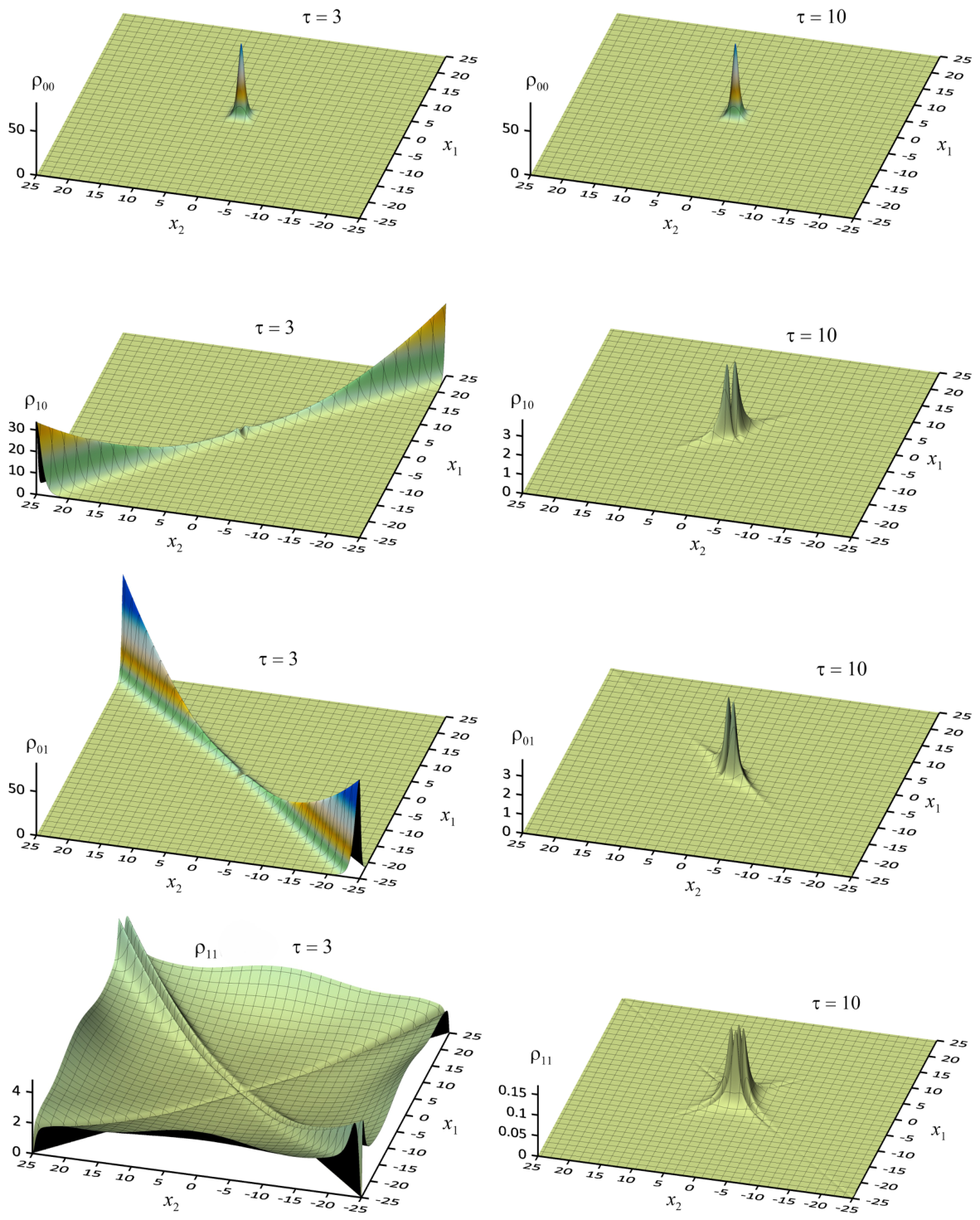
Below in Section 9.3, calculations of the evolution of the elements of the reduced density matrix and their visualization in the form of 3$\mathit{D}$ graphs (see Figure 6).

6. Entropy of a Single Photon Propagating in a Medium

The propagation of a single photon in a nanowaveguide with random influences is a typical irreversible quantum process. Let us recall that such processes are usually studied within the framework of the representation of a non-stationary density matrix, using the Liouville–von Neumann equation [40] or its various generalizations [41,42]. However, there is an important limitation that makes the application of these representations in the case under consideration unsuitable. It should be noted that standard representations of the density matrix take into account the influence of the environment on a quantum system, while the reverse influence, namely the influence on the environment, is not taken into account or is taken into account insufficiently consistently, which in some cases leads to a noticeable loss of information of JS. In other words, these difficulties are insurmountable within the framework of the concept of open quantum systems, since they in any case allow approximate approaches in deriving the master equation.

In the problem under consideration, the photon undergoes multiple scattering, during which it can also be absorbed and emitted by the medium, but in the form of one or two photons with different parameters. In this case, it is obviously necessary to use a representation that takes into account the influence of the quantum system on the environment and does not allow the loss of information about the “QS + environment” joint system (JS).

Following the articles [35,37,39], where the particle and its random environment are considered as a single closed system within the framework of the random matrix method, we can write the form of the stochastic density matrix (SDM):

$$\mathit{\rho }(\mathbf{q},\mathit{\tau };\left\{\mathit{f}\right\}:{\mathbf{q}}^{\prime },{\mathit{\tau }}^{\prime };\left\{{\mathit{f}}^{\prime }\right\})=\sum _{\mathit{n},\mathit{m}}{\mathit{W}}_{\mathit{nm}}{\mathit{\rho }}_{\mathit{nm}}(\mathbf{q},\mathit{\tau };\left\{\mathit{f}\right\}:{\mathbf{q}}^{\prime },{\mathit{\tau }}^{\prime };\left\{{\mathit{f}}^{\prime }\right\}).$$

(91)

In Representation (91), the term ${\mathit{W}}_{\mathit{nm}}$ denotes the population of the levels of two non-interacting quantum harmonic oscillators with energies; ${\mathit{E}}_{\mathit{n}}=(\mathit{n}+\mathbf{1}/\mathbf{2}){\mathit{\omega }}_{\mathbf{1}}^{-}$ and ${\mathit{E}}_{\mathit{m}}=(\mathit{m}+\mathbf{1}/\mathbf{2}){\mathit{\omega }}_{\mathbf{2}}^{-}$. Integrating expression (91) over the coordinates ${\mathit{q}}_{\mathbf{1}},{\mathit{q}}_{\mathbf{2}}\in {\mathbb{R}}^{\mathbf{2}}$, where ${\mathbb{R}}^{\mathbf{2}}$ is a 2$\mathit{D}$ Euclidean subspace, we find the following normalization condition:

$$\sum _{\mathit{n},\mathit{m}}{\mathit{W}}_{\mathit{n},\mathit{m}}=\mathbf{1},{\mathit{W}}_{\mathit{n},\mathit{m}}\ge \mathbf{0}.$$

Using the definition of a random density matrix (91), we can construct a regular reduced density matrix by performing functional integration.

For simplicity, we assume that the population of the quantum levels is such that ${\mathit{W}}_{\mathbf{00}}=\mathbf{1}$ and ${\mathit{W}}_{\mathit{n}\mathit{m}}=\mathbf{0}$, for all integers $\mathit{n},\mathit{m}\ge \mathbf{1}$.

Using the first expression in (88) for the RDM, we can construct the von Neumann entropy, which characterizes the measure of disorder of a QS, i.e., two linearly coupled 1$\mathit{D}$ quantum oscillators in the ground state. Recall that the standard definition of von Neumann entropy is as follows [40]:

$${\mathbf{\Lambda }}_{\mathit{N}}\left(\mathit{\tau }\right)=-{\mathit{Tr}}_{\mathbf{q}}\left\{{\mathit{\rho }}_{\mathbf{00}}(\mathbf{q},\mathit{\tau }:{\mathbf{q}}^{\prime },{\mathit{\tau }}^{\prime })\mathbf{ln}{\mathit{\rho }}_{\mathbf{00}}(\mathbf{q},\mathit{\tau }:{\mathbf{q}}^{\prime },{\mathit{\tau }}^{\prime })\right\}{|}_{{\mathbf{q}}^{\prime }=\mathbf{q};{\mathit{\tau }}^{\prime }=\mathit{\tau }}.$$

(92)

In particular, substituting from (88) first expression for RDM into Equation (92), we can obtain the following expression:

$${\mathbf{\Lambda }}_{\mathit{N}}\left(\mathit{\tau }\right)=-{\mathcal{N}}^{\left(\mathbf{1}\right)}\left(\mathit{\tau }\right){\mathbf{\Lambda }}_{\mathit{N}}^{\left(\mathbf{2}\right)}\left(\mathit{\tau }\right)-{\mathcal{N}}^{\left(\mathbf{2}\right)}\left(\mathit{\tau }\right){\mathbf{\Lambda }}_{\mathit{N}}^{\left(\mathbf{1}\right)}\left(\mathit{\tau }\right),$$

(93)

where ${\mathcal{N}}^{\left(\mathit{l}\right)}\left(\mathit{\tau }\right)$ and ${\mathbf{\Lambda }}_{\mathit{N}}^{\left(\mathit{l}\right)}\left(\mathit{\tau }\right),(\mathit{l}=\mathbf{1},\mathbf{2})$ denote the number of states and the entropy of the $\mathit{l}$-th single oscillator, respectively. Note that the number of states is determined by the following expression:

$$\begin{array}{c}\hfill {\mathcal{N}}^{\left(\mathit{l}\right)}\left(\mathit{\tau }\right)={\int }_{-\infty }^{+\infty }{\mathit{\rho }}_{\mathbf{0}}^{\left(\mathit{l}\right)}({\mathit{q}}_{\mathit{l}},\mathit{\tau }){\mathit{dq}}_{\mathit{j}}={\int }_{-\infty }^{+\infty }{\mathit{du}}_{\mathbf{1}}{\int }_{\mathbf{0}}^{+\infty }{\displaystyle \frac{{\mathit{du}}_{\mathbf{2}}}{\sqrt{{\mathit{u}}_{\mathbf{2}}}}}{\mathcal{P}}_{\mathit{l}}(\mathbf{0};{\mathit{u}}_{\mathbf{1}},{\mathit{u}}_{\mathbf{2}},\mathit{\tau }),\end{array}$$

(94)

where ${\mathit{\rho }}_{\mathbf{0}}^{\left(\mathit{l}\right)}({\mathit{q}}_{\mathit{l}},\mathit{\tau })$ is the RDM of the $\mathit{l}$-th 1$\mathit{D}$-th oscillator, which has the following form:

$${\mathit{\rho }}_{\mathbf{0}}^{\left(\mathit{l}\right)}({\mathit{q}}_{\mathit{l}},\mathit{\tau })={\displaystyle \frac{\mathbf{1}}{\sqrt{\mathit{\pi }}}}{\int }_{-\infty }^{+\infty }{\mathit{du}}_{\mathbf{1}}{\int }_{\mathbf{0}}^{+\infty }{\mathit{du}}_{\mathbf{2}}{\mathcal{P}}_{\mathit{l}}(\mathbf{0};{\mathit{u}}_{\mathbf{1}},{\mathit{u}}_{\mathbf{2}},\mathbf{\tau })\mathbf{exp}\left\{-{\mathit{u}}_{\mathbf{2}}{\mathit{q}}_{\mathit{l}}^{\mathbf{2}}\right\}.$$

As for the entropy of the $\mathit{l}$-th 1$\mathit{D}$-th oscillator, it is determined by the following expression:

$$\begin{array}{c}\hfill {\mathbf{\Lambda }}_{\mathit{N}}^{\left(\mathit{l}\right)}\left(\mathit{\tau }\right)={\int }_{-\infty }^{+\infty }{\mathit{\rho }}_{\mathbf{0}}^{\left(\mathit{l}\right)}({\mathit{q}}_{\mathit{l}},\mathit{\tau })\mathbf{ln}{\mathit{\rho }}_{\mathbf{0}}^{\left(\mathit{l}\right)}({\mathit{q}}_{\mathit{l}},\mathit{\tau }){\mathit{dq}}_{\mathit{l}},\end{array}$$

(95)

As can be seen from Expression (95), the von Neumann entropy has a rather complex form, which does not allow for analytical integration of the expression over the coordinate ${\mathit{q}}_{\mathit{l}}$. However, it should be noted that Definition (95), unlike the standard definition of von Neumann entropy [40], does not fully account for the influence of a QS—in this case, a photon—on its random environment. This is due to the fact that the averaging procedure of a quantum system is carried out only by the distribution ${\mathcal{P}}_{\mathit{l}}(\mathit{n};{\mathit{u}}_{\mathbf{1}},{\mathit{u}}_{\mathbf{2}},\mathit{\tau })$, which does not preserve the full probability in the JS.

Another, more elegant definition of the entropy of a quantum system, where integration over spatial coordinates ${\mathit{q}}_{\mathit{l}}$ can be performed, can be implemented within the framework of the random density matrix method (SDM).

Definition 4. 

The time-dependent entropy of a quantum subsystem immersed in a thermostat can be determined using the mathematical expectation of a random density matrix:

$${\mathbf{\Lambda }}_{\mathit{G}}\left(\mathit{\tau }\right)=-{\mathit{Tr}}_{\mathit{q}}\{{\mathit{Tr}}_{\left\{\mathit{u}\right(\mathit{\tau }\left)\right\}}\left[\mathit{\rho }(\mathit{q},\mathit{\tau };\left\{\mathit{f}\right\}:{\mathit{q}}^{\prime },{\mathit{\tau }}^{\prime };\left\{{\mathit{f}}^{\prime }\right\})\mathbf{ln}\mathit{\rho }(\mathit{q},\mathit{\tau };\left\{\mathit{f}\right\}:{\mathit{q}}^{\prime },{\mathit{\tau }}^{\prime };\left\{{\mathit{f}}^{\prime }\right\})]\right\}.$$

(96)

For definiteness, we will consider the entropy of a photon in the ground state. Given the expression for the random wave function of a single 1$\mathit{D}$ oscillator (73), SDM in the ground state can be written in factorized form:

$$\begin{array}{c}\hfill {\mathit{\rho }}_{\mathbf{00}}(\mathbf{q},\mathit{\tau };\left\{\mathit{f}\right\}:{\mathbf{q}}^{\prime },{\mathit{\tau }}^{\prime };\left\{{\mathit{f}}^{\prime }\right\})={\displaystyle \prod _{\mathit{l}=\mathbf{1}}^{\mathbf{2}}}{\mathit{\rho }}_{\mathbf{0}}^{\left(\mathit{l}\right)}({\mathit{q}}_{\mathit{l}},\mathit{\tau };\left\{\mathit{f}\right\}:{\mathit{q}}_{\mathit{l}}^{\prime },{\mathit{\tau }}^{\prime };\left\{{\mathit{f}}^{\prime }\right\}),\end{array}$$

(97)

where

$${\mathit{\rho }}_{\mathbf{0}}^{\left(\mathit{l}\right)}({\mathit{q}}_{\mathit{l}},\mathit{\tau }:{\mathit{q}}_{\mathit{l}}^{\prime },{\mathit{\tau }}^{\prime })={\displaystyle \frac{\mathbf{1}}{\sqrt{\mathit{\pi }}}}\mathbf{exp}\left\{-{\int }_{\mathbf{0}}^{\mathit{\tau }}{\mathit{u}}_{\mathbf{1}}\left({\mathit{\tau }}^{\prime }\right)\mathit{d}{\mathit{\tau }}^{\prime }-{\displaystyle \frac{\mathbf{1}}{\mathbf{2}}}\left[{\mathit{u}}_{\mathbf{2}}\left(\mathit{\tau }\right){\mathit{q}}_{\mathit{l}}^{\mathbf{2}}+{\mathit{u}}_{\mathbf{2}}\left({\mathit{\tau }}^{\prime }\right){{\mathit{q}}_{\mathit{l}}^{\prime }}^{\mathbf{2}}\right]\right\}.$$

(98)

Substituting (97) into (96) for entropy, we obtain the following expression:

$$\begin{array}{c}\hfill {\mathbf{\Lambda }}_{\mathit{G}}\left(\mathit{\tau }\right)=-{\mathit{Tr}}_{\mathbf{q}}\{{\mathit{Tr}}_{\left\{\mathbf{u}\right(\mathit{\tau }\left)\right\}}\left[{\mathit{\rho }}_{\mathbf{00}}(\mathbf{q},\mathit{\tau };\left\{\mathit{f}\right\}:{\mathbf{q}}^{\prime },{\mathit{\tau }}^{\prime };\left\{{\mathit{f}}^{\prime }\right\})\mathbf{ln}{\mathit{\rho }}_{\mathbf{00}}(\mathbf{q},\mathit{\tau };\left\{\mathit{f}\right\}:{\mathbf{q}}^{\prime },{\mathit{\tau }}^{\prime };\left\{{\mathit{f}}^{\prime }\right\})\right]\\ \hfill =-{\mathit{Tr}}_{\mathbf{q}}\left\{{\mathit{Tr}}_{\left\{\mathbf{u}\right(\mathit{\tau }\left)\right\}}{\mathit{\rho }}_{\mathbf{0}}^{\left(\mathbf{1}\right)}{\mathit{\rho }}_{\mathbf{0}}^{\left(\mathbf{2}\right)}\mathbf{ln}\left[{\mathit{\rho }}_{\mathbf{0}}^{\left(\mathbf{1}\right)}{\mathit{\rho }}_{\mathbf{0}}^{\left(\mathbf{2}\right)}\right]\right\}=-{\mathcal{N}}^{\left(\mathbf{1}\right)}\left(\mathit{\tau }\right){\mathbf{\Lambda }}_{\mathit{G}}^{\left(\mathbf{2}\right)}\left(\mathit{\tau }\right)-{\mathcal{N}}^{\left(\mathbf{2}\right)}\left(\mathit{\tau }\right){\mathbf{\Lambda }}_{\mathit{G}}^{\left(\mathbf{1}\right)}\left(\mathit{\tau }\right),\end{array}$$

(99)

where ${\mathcal{N}}^{\left(\mathit{l}\right)}={\mathit{Tr}}_{{\mathit{q}}_{\mathit{l}}}{\mathit{Tr}}_{\left\{{\mathbf{u}}^{\mathit{l}}\left(\mathit{\tau }\right)\right\}}\left[{\mathit{\rho }}_{\mathbf{0}}^{\left(\mathit{l}\right)}\right]$ and ${\mathbf{\Lambda }}_{\mathit{G}}^{\left(\mathit{l}\right)}={\mathit{Tr}}_{{\mathit{q}}_{\mathit{l}}}{\mathit{Tr}}_{\left\{{\mathbf{u}}^{\mathit{l}}\left(\mathit{\tau }\right)\right\}}\left[{\mathit{\rho }}_{\mathbf{0}}^{\left(\mathit{l}\right)}\mathbf{ln}{\mathit{\rho }}_{\mathbf{0}}^{\left(\mathit{l}\right)}\right]$ are the number of states and the entropy of the $\mathit{l}$-th quantum harmonic oscillator in the ground state, respectively.

In Expression (99), a term of the type ${\mathit{Tr}}_{{\mathit{q}}_{\mathit{l}}}{\mathit{Tr}}_{\left\{{\mathbf{u}}^{\mathit{l}}\left(\mathit{\tau }\right)\right\}}\left[{\mathit{\rho }}_{\mathbf{0}}^{\left(\mathit{l}\right)}\right]$ can be easily calculated. It describes the number of states of 1$\mathit{D}$ QHO in the ground state, which is immersed in a random environment:

$${\mathcal{N}}^{\left(\mathit{l}\right)}\left(\mathit{\tau }\right)={\mathit{Tr}}_{{\mathit{q}}_{\mathit{l}}}\left\{{\mathit{Tr}}_{\left\{{\mathbf{u}}^{\mathit{l}}\left(\mathit{\tau }\right)\right\}}{\mathit{\rho }}_{\mathbf{0}}^{\left(\mathit{l}\right)}\right\}={\int }_{-\infty }^{+\infty }{\mathit{du}}_{\mathbf{1}}{\int }_{\mathbf{0}}^{+\infty }{\mathit{du}}_{\mathbf{2}}{\displaystyle \frac{\mathbf{1}}{\sqrt{{\mathit{u}}_{\mathbf{2}}}}}{\mathcal{P}}_{\mathit{l}}(\mathbf{0};{\mathit{u}}_{\mathbf{1}},{\mathit{u}}_{\mathbf{2}},\mathit{\tau }).$$

(100)

The term of type ${\mathbf{\Lambda }}^{\left(\mathit{l}\right)}\left(\mathit{\tau }\right)={\mathit{Tr}}_{{\mathit{q}}_{\mathit{l}}}\left\{{\mathit{Tr}}_{\left\{{\mathbf{u}}^{\mathit{l}}\left(\mathit{\tau }\right)\right\}}{\mathit{\rho }}_{\mathbf{0}}^{\left(\mathit{l}\right)}\mathbf{ln}{\mathit{\rho }}_{\mathbf{0}}^{\left(\mathit{l}\right)}\right\}$ in Expression (99) represents the entropy of one 1$\mathit{D}$ quantum oscillator, which can be written as follows:

$$\begin{array}{c}\hfill {\mathbf{\Lambda }}^{\left(\mathit{l}\right)}\left(\mathit{\tau }\right)=-{\displaystyle \frac{\mathbf{1}}{\sqrt{\mathit{\pi }}}}{\mathit{Tr}}_{{\mathit{q}}_{\mathit{l}}}{\mathit{Tr}}_{\left\{{\mathbf{u}}^{\mathit{l}}\left(\mathit{\tau }\right)\right\}}\left\{{\mathit{e}}^{-{\int }_{\mathbf{0}}^{\mathit{\tau }}{\mathit{u}}_{\mathbf{1}}\left({\mathit{\tau }}^{\prime }\right)\mathit{d}{\mathit{\tau }}^{\prime }-{\mathit{u}}_{\mathbf{2}}{\mathit{q}}_{\mathit{l}}^{\mathbf{2}}}\left[{\mathit{u}}_{\mathbf{2}}{\mathit{q}}_{\mathit{l}}^{\mathbf{2}}+{\int }_{\mathbf{0}}^{\mathit{\tau }}{\mathit{u}}_{\mathbf{1}}\left({\mathit{\tau }}^{\prime }\right)\mathit{d}{\mathit{\tau }}^{\prime }\right]\right\}\\ \hfill =-{\displaystyle \frac{\mathbf{1}}{\mathbf{2}}}{\mathcal{N}}^{\left(\mathit{l}\right)}\left(\mathit{\tau }\right)-{\displaystyle \frac{\mathbf{1}}{\sqrt{\mathit{\pi }}}}{\mathit{Tr}}_{{\mathit{q}}_{\mathit{l}}}{\mathit{Tr}}_{\left\{{\mathbf{u}}^{\mathit{l}}\left(\mathit{\tau }\right)\right\}}\left\{{\mathit{e}}^{-{\int }_{\mathbf{0}}^{\mathit{\tau }}{\mathit{u}}_{\mathbf{1}}\left({\mathit{\tau }}^{\prime }\right)\mathit{d}{\mathit{\tau }}^{\prime }}\left[{\int }_{\mathbf{0}}^{\mathit{\tau }}{\mathit{u}}_{\mathbf{1}}\left({\mathit{\tau }}^{\prime }\right)\mathit{d}{\mathit{\tau }}^{\prime }\right]\right\}.\end{array}$$

(101)

Now, let us move on to the question of calculating the second term in Expression (101), namely the following function:

$${\mathcal{I}}^{\left(\mathit{l}\right)}\left(\mathit{\tau }\right)={\displaystyle \frac{\mathbf{1}}{\sqrt{\mathit{\pi }}}}{\mathit{Tr}}_{{\mathit{q}}_{\mathit{l}}}{\mathit{Tr}}_{\left\{{\mathbf{u}}^{\mathit{l}}\left(\mathit{\tau }\right)\right\}}\left\{{\mathit{e}}^{-{\int }_{\mathbf{0}}^{\mathit{\tau }}{\mathit{u}}_{\mathbf{1}}\left({\mathit{\tau }}^{\prime }\right)\mathit{d}{\mathit{\tau }}^{\prime }}\left[{\int }_{\mathbf{0}}^{\mathit{\tau }}{\mathit{u}}_{\mathbf{1}}\left({\mathit{\tau }}^{\prime }\right)\mathit{d}{\mathit{\tau }}^{\prime }\right]\right\}.$$

Note that ${\mathcal{I}}^{\left(\mathit{l}\right)}\left(\mathit{\tau }\right)={\partial }_{\mathit{\lambda }}{\mathcal{I}}^{\left(\mathit{l}\right)}(\mathit{\lambda };\mathit{\tau }){|}_{\mathit{\lambda }=\mathbf{0}}$, where ${\mathcal{I}}^{\left(\mathit{l}\right)}(\mathit{\lambda };\mathit{\tau })$ has the form:

$$\begin{array}{c}\hfill {\mathcal{I}}^{\left(\mathit{l}\right)}(\mathit{\lambda };\mathit{\tau })={\displaystyle \frac{\mathbf{1}}{\sqrt{\mathit{\pi }}}}{\mathit{Tr}}_{{\mathit{q}}_{\mathit{l}}}{\mathit{Tr}}_{\left\{{\mathbf{u}}^{\mathit{l}}\left(\mathit{\tau }\right)\right\}}\left\{{\mathit{e}}^{-(\mathbf{1}+\mathit{\lambda }){\int }_{\mathbf{0}}^{\mathit{\tau }}{\mathit{u}}_{\mathbf{1}}\left({\mathit{\tau }}^{\prime }\right)\mathit{d}{\mathit{\tau }}^{\prime }-{\mathit{u}}_{\mathbf{2}}{\mathit{q}}_{\mathit{l}}^{\mathbf{2}}}\right\}.\end{array}$$

(102)

Integrating over the ${\mathit{q}}_{\mathit{l}}$ coordinate into expression (102), we find:

$${\mathcal{I}}^{\left(\mathit{l}\right)}(\mathit{\lambda };\mathit{\tau })={\displaystyle \frac{\mathbf{1}}{\sqrt{{\mathit{u}}_{\mathbf{2}}}}}{\mathit{Tr}}_{\left\{{\mathbf{u}}^{\mathit{l}}\left(\mathit{\tau }\right)\right\}}\left\{{\mathit{e}}^{-(\mathbf{1}+\mathit{\lambda }){\int }_{\mathbf{0}}^{\mathit{\tau }}{\mathit{u}}_{\mathbf{1}}\left({\mathit{\tau }}^{\prime }\right)\mathit{d}{\mathit{\tau }}^{\prime }}\right\}.$$

(103)

Finally, performing functional integration in (103) we obtain:

$${\mathcal{I}}^{\left(\mathit{l}\right)}(\mathit{\lambda };\mathit{\tau })={\int }_{-\infty }^{+\infty }{\mathit{du}}_{\mathbf{1}}{\int }_{\mathbf{0}}^{\infty }{\mathit{du}}_{\mathbf{2}}{\displaystyle \frac{\mathbf{1}}{\sqrt{{\mathit{u}}_{\mathbf{2}}}}}{\mathcal{P}}_{\mathit{l}}(\mathit{\lambda };{\mathit{u}}_{\mathbf{1}},{\mathit{u}}_{\mathbf{2}},\mathit{\tau }),$$

(104)

where the integrand function ${\mathcal{P}}_{\mathit{l}}(\mathit{\lambda };{\mathit{u}}_{\mathbf{1}},{\mathit{u}}_{\mathbf{2}},\mathit{\tau })$ satisfies the following PDE:

$$\left\{{\partial }_{\mathit{\tau }}-{\widehat{\mathit{L}}}_{\mathit{l}}+(\mathbf{1}+\mathit{\lambda }){\mathit{u}}_{\mathbf{1}}\right\}{\mathcal{P}}_{\mathit{l}}(\mathit{\lambda };{\mathit{u}}_{\mathbf{1}},{\mathit{u}}_{\mathbf{2}},\mathit{\tau })=\mathbf{0}.$$

(105)

Taking into account the definition of the function ${\mathcal{I}}^{\left(\mathit{l}\right)}\left(\mathit{\tau }\right)$, we can write:

$${\mathcal{I}}^{\left(\mathit{l}\right)}\left(\mathit{\tau }\right)={\int }_{-\infty }^{+\infty }{\mathit{du}}_{\mathbf{1}}{\int }_{\mathbf{0}}^{\infty }{\mathit{du}}_{\mathbf{2}}{\displaystyle \frac{\mathbf{1}}{\sqrt{{\mathit{u}}_{\mathbf{2}}}}}{\mathcal{D}}_{\mathit{l}}(\mathbf{0};{\mathit{u}}_{\mathbf{1}},{\mathit{u}}_{\mathbf{2}},\mathit{\tau }),$$

(106)

where ${\mathcal{D}}_{\mathit{l}}(\mathbf{0};{\mathit{u}}_{\mathbf{1}},{\mathit{u}}_{\mathbf{2}},\mathit{\tau })={\partial }_{\mathit{\lambda }}{\mathcal{P}}_{\mathit{l}}(\mathit{\lambda };{\mathit{u}}_{\mathbf{1}},{\mathit{u}}_{\mathbf{2}},\mathit{\tau }){|}_{\mathit{\lambda }=\mathbf{0}}.$

Now, taking into account (105), it is easy to prove that the function $\mathcal{D}(\mathbf{0};{\mathit{u}}_{\mathbf{1}},{\mathit{u}}_{\mathbf{2}},\mathit{\tau })$ is a solution to the following non-homogeneous PDE:

$$\{{\partial }_{\mathit{\tau }}-{\widehat{\mathit{L}}}_{\mathit{l}}+{\mathit{u}}_{\mathbf{1}}\}{\mathcal{D}}_{\mathit{l}}(\mathbf{0};{\mathit{u}}_{\mathbf{1}},{\mathit{u}}_{\mathbf{2}},\mathit{\tau })+{\mathit{u}}_{\mathbf{1}}{\mathcal{P}}_{\mathit{l}}(\mathbf{0};{\mathit{u}}_{\mathbf{1}},{\mathit{u}}_{\mathbf{2}},\mathit{\tau })=\mathbf{0}.$$

(107)

As can be easily verified, Equation (107) involves a source ${\mathcal{P}}_{\mathit{l}}(\mathbf{0};{\mathit{u}}_{\mathbf{1}},{\mathit{u}}_{\mathbf{2}},\mathit{\tau })$ that obeys the wave Equation (89), and so to find a solution ${\mathcal{D}}_{\mathit{l}}(\mathbf{0};{\mathit{u}}_{\mathbf{1}},{\mathit{u}}_{\mathbf{2}},\mathit{\tau })$, we need to solve (107) and (89) together, self-consistently. The entropy of the $\mathit{l}$-th 1$\mathit{D}$ quantum harmonic oscillator will have the following form:

$${\mathbf{\Lambda }}^{\left(\mathit{l}\right)}\left(\mathit{\tau }\right)=-{\displaystyle \frac{\mathbf{1}}{\mathbf{2}}}{\mathcal{N}}^{\left(\mathit{l}\right)}-{\mathcal{I}}^{\left(\mathit{l}\right)}\left(\mathit{\tau }\right).$$

(108)

Thus, we have defined two different types of time-dependent entropies for a QS, ${\mathbf{\Lambda }}_{\mathit{N}}\left(\mathit{\tau }\right)$ and ${\mathbf{\Lambda }}_{\mathit{G}}\left(\mathit{\tau }\right)$, which do not take into account the influence of the quantum system on the environment. In other words, these entropies describe open systems and are inaccurate in the case of strong interactions between the QS and its environment. This problem can be solved—that is, the question of conserving total probability in a self-organizing closed system (see definition of JS)—by radically changing the definition of entropy, using the mathematical expectation of the photon’s wave function.

Definition 5. 

The time-dependent entropy of a quantum subsystem self-organizing in a random environment will be denoted by the following expression:

$${\mathbf{\Lambda }}_{\mathit{S}}\left(\mathit{\tau }\right)=-{\mathit{Tr}}_{\mathit{q}}\left\{\mathit{\varrho }\left(\mathit{n}\right|\mathit{q},\mathit{\tau }:{\mathit{q}}^{\prime },{\mathit{\tau }}^{\prime })\mathbf{ln}\mathit{\varrho }\left(\mathit{n}\right|\mathit{q},\mathit{\tau }:{\mathit{q}}^{\prime },{\mathit{\tau }}^{\prime })\right\},$$

(109)

where $\mathit{\varrho }\left(\mathit{n}\right|\mathit{q},\mathit{\tau }:{\mathit{q}}^{\prime },{\mathit{\tau }}^{\prime })$ denotes the mathematical expectation of RDM, which is defined by the following bilinear form (see Expressions (74)–(77)); in addition, $\mathit{n}={\mathit{n}}_{\mathbf{1}},{\mathit{n}}_{\mathbf{2}}$ are quantum numbers:

$$\mathit{\varrho }\left(\mathit{n}\right|\mathit{q},\mathit{\tau }:{\mathit{q}}^{\prime },{\mathit{\tau }}^{\prime }){|}_{\mathit{q}={\mathit{q}}^{\prime };\mathit{\tau }={\mathit{\tau }}^{\prime }}={\displaystyle \prod _{\mathit{l}=\mathbf{1}}^{\mathbf{2}}}{\overline{\mathcal{F}}}_{\mathit{l}}\left({\mathit{n}}_{\mathit{l}}\right|{\mathit{q}}_{\mathit{l}},\mathit{\tau })·{\overline{\mathcal{F}}}_{\mathit{l}}^{*}\left({\mathit{n}}_{\mathit{l}}\right|{\mathit{q}}_{\mathit{l}},\mathit{\tau }).$$

(110)

Below, for definiteness, we will consider the entropy of a single photon in the ground state during the relaxation process in the random environment.

Substituting the representation for RDM (110) into Equation (109), we obtain the following expression for the entropy QS:

$${\mathbf{\Lambda }}_{\mathit{S}}\left(\mathit{\tau }\right)=-{\mathcal{N}}_{\mathit{S}}^{\left(\mathbf{1}\right)}\left(\mathit{\tau }\right){\mathbf{\Lambda }}_{\mathit{S}}^{\left(\mathbf{2}\right)}\left(\mathit{\tau }\right)-{\mathcal{N}}_{\mathit{S}}^{\left(\mathbf{2}\right)}\left(\mathit{\tau }\right){\mathbf{\Lambda }}_{\mathit{S}}^{\left(\mathbf{1}\right)}\left(\mathit{\tau }\right),$$

(111)

where ${\mathcal{N}}_{\mathit{S}}^{\left(\mathit{l}\right)}\left(\mathit{\tau }\right)$ and ${\mathbf{\Lambda }}_{\mathbf{S}}^{\left(\mathit{l}\right)}\left(\mathit{\tau }\right)$ denote, respectively, the density of states and the entropy of the $\mathit{l}$-th 1$\mathit{D}$ QHO, which are defined by following expressions:

$${\mathcal{N}}_{\mathit{S}}^{\left(\mathit{l}\right)}\left(\mathit{\tau }\right)={\displaystyle \underset{-\infty }{\overset{+\infty }{\int }}}{\mathit{dq}}_{\mathit{l}}{\mathit{\varrho }}_{\mathit{l}}\left(\mathbf{0}\right|{\mathit{q}}_{\mathit{l}},\mathit{\tau })={\displaystyle \underset{-\infty }{\overset{+\infty }{\int }}}{\overline{\mathcal{F}}}_{\mathit{l}}\left(\mathbf{0}\right|{\mathit{q}}_{\mathit{l}},\mathit{\tau })·{\overline{\mathcal{F}}}_{\mathit{l}}^{*}\left(\mathbf{0}\right|{\mathit{q}}_{\mathit{l}},\mathit{\tau }){\mathit{dq}}_{\mathit{l}},$$

(112)

and accordingly:

$$\begin{array}{c}\hfill {\mathbf{\Lambda }}_{\mathit{S}}^{\left(\mathit{l}\right)}\left(\mathit{\tau }\right)={\displaystyle \underset{-\infty }{\overset{+\infty }{\int }}}{\mathit{dq}}_{\mathit{l}}{\mathit{\varrho }}_{\mathit{l}}\left(\mathbf{0}\right|{\mathit{q}}_{\mathit{l}},\mathit{\tau })\mathbf{ln}{\mathit{\varrho }}_{\mathit{l}}\left(\mathbf{0}\right|{\mathit{q}}_{\mathit{l}},\mathit{\tau })=\\ \hfill {\displaystyle \underset{-\infty }{\overset{+\infty }{\int }}}{\overline{\mathcal{F}}}_{\mathit{l}}\left(\mathbf{0}\right|{\mathit{q}}_{\mathit{l}},\mathit{\tau })·{\overline{\mathcal{F}}}_{\mathit{l}}^{*}\left(\mathbf{0}\right|{\mathit{q}}_{\mathit{l}},\mathit{\tau })\mathbf{ln}\left\{{\overline{\mathcal{F}}}_{\mathit{l}}\left(\mathbf{0}\right|{\mathit{q}}_{\mathit{l}},\mathit{\tau })·{\overline{\mathcal{F}}}_{\mathit{l}}^{*}\left(\mathbf{0}\right|{\mathit{q}}_{\mathit{l}},\mathit{\tau })\right\}{\mathit{dq}}_{\mathit{l}}.\end{array}$$

(113)

Using the expression for the mathematical expectation of the photon wave function (74), we can calculate the coefficient ${\mathcal{N}}_{\mathit{S}}^{\left(\mathit{l}\right)}\left(\mathit{\tau }\right)$ and represent it as a four-dimensional integral representation:

$$\begin{array}{c}\hfill {\mathcal{N}}_{\mathit{S}}^{\left(\mathit{l}\right)}\left(\mathit{\tau }\right)=\sqrt{\mathbf{2}}{\displaystyle \underset{-\infty }{\overset{+\infty }{\int }}}{\mathit{du}}_{\mathbf{1}}{\displaystyle \underset{\mathbf{0}}{\overset{+\infty }{\int }}}{\mathit{du}}_{\mathbf{2}}{\displaystyle \underset{-\infty }{\overset{+\infty }{\int }}}\mathit{d}{\overline{\mathit{u}}}_{\mathbf{1}}{\displaystyle \underset{\mathbf{0}}{\overset{+\infty }{\int }}}\mathit{d}{\overline{\mathit{u}}}_{\mathbf{2}}{\displaystyle \frac{{\mathit{Q}}_{\mathit{l}}(\mathbf{0};{\mathit{u}}_{\mathbf{1}},{\mathit{u}}_{\mathbf{2}},\mathit{\tau }){\mathit{Q}}_{\mathit{l}}^{*}(\mathbf{0};{\overline{\mathit{u}}}_{\mathbf{1}},{\overline{\mathit{u}}}_{\mathbf{2}},\mathit{\tau })}{\sqrt{({\mathit{u}}_{\mathbf{2}}+{\overline{\mathit{u}}}_{\mathbf{2}})+\mathit{i}({\mathit{u}}_{\mathbf{1}}-{\overline{\mathit{u}}}_{\mathbf{1}})}}},\end{array}$$

(114)

where

$${\mathit{Q}}_{\mathit{l}}(\mathbf{0};{\mathit{u}}_{\mathbf{1}},{\mathit{u}}_{\mathbf{2}},\mathit{\tau }){\mathit{Q}}_{\mathit{l}}^{\left(\mathit{i}\right)}{\mathit{Q}}_{\mathit{l}}^{*}(\mathbf{0};{\overline{\mathit{u}}}_{\mathbf{1}},{\overline{\mathit{u}}}_{\mathbf{2}},\mathit{\tau })=$$

$${\mathit{Q}}_{\mathit{l}}^{\left(\mathit{r}\right)}(\mathbf{0};{\mathit{u}}_{\mathbf{1}},{\mathit{u}}_{\mathbf{2}},\mathit{\tau }){\mathit{Q}}_{\mathit{l}}^{\left(\mathit{r}\right)}(\mathbf{0};{\overline{\mathit{u}}}_{\mathbf{1}},{\overline{\mathit{u}}}_{\mathbf{2}},\mathit{\tau })+{\mathit{Q}}_{\mathit{l}}^{\left(\mathit{i}\right)}(\mathbf{0};{\mathit{u}}_{\mathbf{1}},{\mathit{u}}_{\mathbf{2}},\mathit{\tau }){\mathit{Q}}_{\mathit{l}}^{\left(\mathit{i}\right)}(\mathbf{0};{\overline{\mathit{u}}}_{\mathbf{1}},{\overline{\mathit{u}}}_{\mathbf{2}},\mathit{\tau })-$$

$${\mathit{iQ}}_{\mathit{l}}^{\left(\mathit{r}\right)}(\mathbf{0};{\mathit{u}}_{\mathbf{1}},{\mathit{u}}_{\mathbf{2}},\mathit{\tau }){\mathit{Q}}_{\mathit{l}}^{\left(\mathit{i}\right)}(\mathbf{0};{\overline{\mathit{u}}}_{\mathbf{1}},{\overline{\mathit{u}}}_{\mathbf{2}},\mathit{\tau })+{\mathit{iQ}}_{\mathit{l}}^{\left(\mathit{i}\right)}(\mathbf{0};{\mathit{u}}_{\mathbf{1}},{\mathit{u}}_{\mathbf{2}},\mathit{\tau }){\mathit{Q}}_{\mathit{l}}^{\left(\mathit{r}\right)}(\mathbf{0};{\overline{\mathit{u}}}_{\mathbf{1}},{\overline{\mathit{u}}}_{\mathbf{2}},\mathit{\tau }).$$

Note that Expression (114) defining the density of states is, by definition, a positive real quantity.

Unfortunately, it is not possible to carry out analytical integration of the expression for the entropy of an individual photon (113) over the ${\mathit{q}}_{\mathit{l}}$ coordinate, which greatly complicates its numerical calculation.

Thus, we have constructed the entropy of a system of photons using the standard von Neumann definition (95), the SDM method, and in the framework of the mathematical expectation of the photon wave function (109) and (110). Thus, we have constructed the entropy of a system of photons using the standard von Neumann definition (95), the SDM method, and within the ME method of the photon wave function (109) and (110). Under certain conditions, a single-photon system can decay into two photons, and the state of each individual photon will be described by the wave function of a 1$\mathit{D}$ QHO immersed in a random environment. The difference between these representations is that in the framework of the ME method for the wave function, the influence of the quantum system on the environment is correctly taken into account, which is fundamentally important in the case of strong interaction between the quantum system and its environment.

An important feature of Expressions (95) and (113) is that, as can be seen, if they characterize the evolution of a system of two single photons, then these photons are obviously entangled through the entropies of the individual photons.

7. Transition Probabilities to Bell States

Let us consider a problem where a photon, moving in a nanowaveguide, is scattered by quantum dots randomly located along its trajectory. Clearly, in this case, as a result of inelastic scattering, there is a possibility of the photon being absorbed by the quantum dot, which will eventually emit two entangled photons. For the organization of quantum communications using photons, the degree of their entanglement plays a very important role. In particular, maximum entanglement between photons is achieved using four so-called Bell states (see for example [43,44]).

Mathematically, single-photon states, taking into account their helicity, in a plane perpendicular to the direction of photon propagation, can be represented as two-component vector wave functions of the form:

$$|\mathbf{1}\rangle =\left(\begin{array}{c}{|\mathbf{1}\rangle }_{\uparrow }\\ {|\mathbf{1}\rangle }_{\downarrow }\end{array}\right),|\mathbf{2}\rangle =\left(\begin{array}{c}{|\mathbf{2}\rangle }_{\uparrow }\\ {|\mathbf{2}\rangle }_{\downarrow }\end{array}\right),$$

(115)

where $|\mathbf{1}\rangle =|{\mathbf{r}}_{\mathbf{1}}\rangle$ and $|\mathbf{2}\rangle =|{\mathbf{r}}_{\mathbf{2}}\rangle$ denote the singlet wave functions of the first and second photons, respectively, ${\mathbf{r}}_{\mathbf{1}},{\mathbf{r}}_{\mathbf{2}}\in {\mathbb{R}}^{\mathbf{2}}$ denote the radius vectors of localization of the corresponding photons, ${|\mathit{l}\rangle }_{\uparrow }$ and ${|\mathit{l}\rangle }_{\downarrow }(\mathit{l}=\mathbf{1},\mathbf{2})$ denote photons with right and left polarization, respectively. Taking into account the above, we can write down all four time-like Bell states that describe the maximally entangled state of two qubits and form an orthogonal basis in the Hilbert space:

$$\begin{array}{c}\hfill |{\mathit{\psi }}_{\pm }\rangle ={\displaystyle \frac{\mathbf{1}}{\sqrt{\mathbf{2}}}}\left\{{|\mathbf{1}\rangle }_{\uparrow }\otimes {|\mathbf{2}\rangle }_{\uparrow }\pm {|\mathbf{1}\rangle }_{\downarrow }\otimes {|\mathbf{2}\rangle }_{\downarrow }\right\},\\ \hfill |{\mathit{\varphi }}_{\pm }\rangle ={\displaystyle \frac{\mathbf{1}}{\sqrt{\mathbf{2}}}}\left\{{|\mathbf{1}\rangle }_{\uparrow }\otimes {|\mathbf{2}\rangle }_{\downarrow }\pm {|\mathbf{1}\rangle }_{\downarrow }\otimes {|\mathbf{2}\rangle }_{\uparrow }\right\}.\end{array}$$

(116)

Using the Riemann–Silberstein vector representation [32,33] for two right-handed (left-handed) helicities of photons simultaneously localized in two different spatial positions ${\mathbf{r}}_{\mathbf{1}}={\mathbf{r}}_{\mathbf{1}}({\mathit{x}}_{\mathbf{1}},{\mathit{x}}_{\mathbf{2}})$ and ${\mathbf{r}}_{\mathbf{2}}={\mathbf{r}}_{\mathbf{2}}({\mathit{x}}_{\mathbf{1}},{\mathit{x}}_{\mathbf{2}})$ at time “$\mathit{\tau }$” (see also expression (10)), the wave functions can be written as follows:

$$\begin{array}{c}\hfill {|\mathbf{1}\rangle }_{\uparrow \downarrow }=\left\{{\displaystyle \frac{{\mathbf{D}}_{\mathbf{1}}\left({\mathbf{r}}_{\mathbf{1}}\right)}{\sqrt{\mathit{\epsilon }\left({\mathbf{r}}_{\mathbf{1}}\right)}}}\pm \mathit{i}{\displaystyle \frac{{\mathbf{B}}_{\mathbf{1}}\left({\mathbf{r}}_{\mathbf{1}}\right)}{\sqrt{\mathit{\mu }\left({\mathbf{r}}_{\mathbf{1}}\right)}}}\right\},{|\mathbf{2}\rangle }_{\uparrow \downarrow }=\left\{{\displaystyle \frac{{\mathbf{D}}_{\mathbf{2}}\left({\mathbf{r}}_{\mathbf{2}}\right)}{\sqrt{\mathit{\epsilon }\left({\mathbf{r}}_{\mathbf{2}}\right)}}}\pm \mathbf{i}{\displaystyle \frac{{\mathbf{B}}_{\mathbf{2}}\left({\mathbf{r}}_{\mathbf{2}}\right)}{\sqrt{\mathit{\mu }\left({\mathbf{\rho }}_{\mathbf{2}}\right)}}}\right\}.\end{array}$$

(117)

Using (117), we can easily construct the wave functions of all two-photon states, namely: $\left\{{|\mathbf{1}\rangle }_{\uparrow }\otimes {|\mathbf{2}\rangle }_{\uparrow }{;|\mathbf{1}\rangle }_{\downarrow }\otimes {|\mathbf{2}\rangle }_{\downarrow }{;|\mathbf{1}\rangle }_{\uparrow }\otimes {|\mathbf{2}\rangle }_{\downarrow }{;|\mathbf{1}\rangle }_{\downarrow }\otimes {|\mathbf{2}\rangle }_{\uparrow }\right\}$ and, with their help, the corresponding Bell states (116).

Taking into account above, the Bell states (116) can be rewritten in the following form:

$$\begin{array}{c}\hfill |{\mathit{\psi }}_{+}\rangle =\sqrt{\mathbf{2}}\left\{{\displaystyle \frac{{\mathbf{D}}_{\mathbf{1}}\left({\mathit{\rho }}_{\mathbf{1}}\right)\otimes {\mathbf{D}}_{\mathbf{2}}\left({\mathbf{r}}_{\mathbf{2}}\right)}{\sqrt{\mathit{\epsilon }\left({\mathbf{r}}_{\mathbf{1}}\right)\mathit{\epsilon }\left({\mathbf{r}}_{\mathbf{2}}\right)}}}-{\displaystyle \frac{{\mathbf{B}}_{\mathbf{1}}\left({\mathbf{r}}_{\mathbf{1}}\right)\otimes {\mathbf{B}}_{\mathbf{2}}\left({\mathbf{r}}_{\mathbf{2}}\right)}{\sqrt{\mathit{\mu }\left({\mathbf{r}}_{\mathbf{1}}\right)\mathit{\mu }\left({\mathbf{r}}_{\mathbf{2}}\right)}}}\right\},\\ \hfill |{\mathit{\psi }}_{-}\rangle =\mathit{i}\sqrt{\mathbf{2}}\left\{{\displaystyle \frac{{\mathbf{D}}_{\mathbf{1}}\left({\mathbf{r}}_{\mathbf{1}}\right)\otimes {\mathbf{B}}_{\mathbf{2}}\left({\mathbf{r}}_{\mathbf{2}}\right)}{\sqrt{\mathit{\epsilon }\left({\mathbf{r}}_{\mathbf{1}}\right)\mathit{\mu }\left({\mathbf{r}}_{\mathbf{2}}\right)}}}+{\displaystyle \frac{{\mathbf{B}}_{\mathbf{1}}\left({\mathbf{r}}_{\mathbf{1}}\right)\otimes {\mathbf{D}}_{\mathbf{2}}\left({\mathbf{r}}_{\mathbf{2}}\right)}{\sqrt{\mathit{\epsilon }\left({\mathbf{r}}_{\mathbf{2}}\right)\mathit{\mu }\left({\mathbf{r}}_{\mathbf{1}}\right)}}}\right\},\\ \hfill |{\mathit{\varphi }}_{+}\rangle =\sqrt{\mathbf{2}}\left\{{\displaystyle \frac{{\mathbf{D}}_{\mathbf{1}}\left({\mathbf{r}}_{\mathbf{1}}\right)\otimes {\mathbf{D}}_{\mathbf{2}}\left({\mathbf{r}}_{\mathbf{2}}\right)}{\sqrt{\mathit{\epsilon }\left({\mathbf{r}}_{\mathbf{1}}\right)\mathit{\epsilon }\left({\mathbf{r}}_{\mathbf{2}}\right)}}}+{\displaystyle \frac{{\mathbf{B}}_{\mathbf{1}}\left({\mathbf{r}}_{\mathbf{1}}\right)\otimes {\mathbf{B}}_{\mathbf{2}}\left({\mathbf{r}}_{\mathbf{2}}\right)}{\sqrt{\mathit{\mu }\left({\mathbf{r}}_{\mathbf{1}}\right)\mathit{\mu }\left({\mathbf{r}}_{\mathbf{2}}\right)}}}\right\},\\ \hfill |{\mathit{\psi }}_{-}\rangle =\mathit{i}\sqrt{\mathbf{2}}\left\{{\displaystyle \frac{{\mathbf{D}}_{\mathbf{1}}\left({\mathbf{r}}_{\mathbf{1}}\right)\otimes {\mathbf{B}}_{\mathbf{2}}\left({\mathbf{r}}_{\mathbf{2}}\right)}{\sqrt{\mathit{\epsilon }\left({\mathbf{r}}_{\mathbf{1}}\right)\mathit{\mu }\left({\mathbf{r}}_{\mathbf{2}}\right)}}}-{\displaystyle \frac{{\mathbf{B}}_{\mathbf{1}}\left({\mathbf{r}}_{\mathbf{1}}\right)\otimes {\mathbf{D}}_{\mathbf{2}}\left({\mathbf{r}}_{\mathbf{2}}\right)}{\sqrt{\mathit{\epsilon }\left({\mathbf{r}}_{\mathbf{2}}\right)\mathit{\mu }\left({\mathbf{r}}_{\mathbf{1}}\right)}}}\right\}.\end{array}$$

(118)

The electric and magnetic field strengths of photons can be represented in vector form. In particular, for the first photon, this will look like:

$${\mathbf{D}}_{\mathbf{1}}\left({\mathbf{r}}_{\mathbf{1}}\right)=\left(\begin{array}{c}{\mathit{D}}_{\mathbf{1}}\left({\mathit{x}}_{\mathbf{1}}\right)\\ \mathbf{0}\end{array}\right),{\mathbf{B}}_{\mathbf{1}}\left({\mathbf{r}}_{\mathbf{1}}\right)=\left(\begin{array}{c}{\mathit{B}}_{\mathbf{1}}\left({\mathit{x}}_{\mathbf{1}}\right)\\ \mathbf{0}\end{array}\right),$$

(119)

and for the second photon, respectively:

$${\mathbf{D}}_{\mathbf{2}}\left({\mathbf{r}}_{\mathbf{2}}\right)=\left(\begin{array}{c}{\mathit{D}}_{\mathbf{2}}\left({\mathit{x}}_{\mathbf{2}}\right)\\ \mathbf{0}\end{array}\right),{\mathbf{B}}_{\mathbf{2}}\left({\mathbf{r}}_{\mathbf{2}}\right)=\left(\begin{array}{c}{\mathit{B}}_{\mathbf{2}}\left({\mathit{x}}_{\mathbf{2}}\right)\\ \mathbf{0}\end{array}\right).$$

(120)

Now, using Expressions (119) and (120), Equation (118) can be written explicitly:

$$\begin{array}{c}\hfill |{\mathit{\psi }}_{+}\rangle =\sqrt{\mathbf{2}}\left\{{\displaystyle \frac{{\mathit{D}}_{\mathbf{1}}\left({\mathit{x}}_{\mathbf{1}}\right){\mathit{D}}_{\mathbf{2}}\left({\mathit{x}}_{\mathbf{2}}\right)}{\sqrt{\mathit{\epsilon }\left({\mathit{x}}_{\mathbf{1}}\right)\mathit{\epsilon }\left({\mathit{x}}_{\mathbf{2}}\right)}}}-{\displaystyle \frac{{\mathit{B}}_{\mathbf{1}}\left({\mathit{x}}_{\mathbf{1}}\right){\mathit{B}}_{\mathbf{2}}\left({\mathit{x}}_{\mathbf{2}}\right)}{\sqrt{\mathit{\mu }\left({\mathit{x}}_{\mathbf{1}}\right)\mathit{\mu }\left({\mathit{x}}_{\mathbf{2}}\right)}}}\right\},\\ \hfill |{\mathit{\psi }}_{-}\rangle =\mathit{i}\sqrt{\mathbf{2}}\left\{{\displaystyle \frac{{\mathit{D}}_{\mathbf{1}}\left({\mathit{x}}_{\mathbf{1}}\right){\mathit{B}}_{\mathbf{2}}\left({\mathit{x}}_{\mathbf{2}}\right)}{\sqrt{\mathit{\epsilon }\left({\mathit{x}}_{\mathbf{1}}\right)\mathit{\mu }\left({\mathit{x}}_{\mathbf{2}}\right)}}}+{\displaystyle \frac{{\mathit{B}}_{\mathbf{1}}\left({\mathit{x}}_{\mathbf{1}}\right){\mathit{D}}_{\mathbf{2}}\left({\mathit{x}}_{\mathbf{2}}\right)}{\sqrt{\mathit{\mu }\left({\mathit{x}}_{\mathbf{1}}\right)\mathit{\epsilon }\left({\mathit{x}}_{\mathbf{2}}\right)}}}\right\},\\ \hfill |{\mathit{\varphi }}_{+}\rangle =\sqrt{\mathbf{2}}\left\{{\displaystyle \frac{{\mathit{D}}_{\mathbf{1}}\left({\mathit{x}}_{\mathbf{1}}\right){\mathit{D}}_{\mathbf{2}}\left({\mathit{x}}_{\mathbf{2}}\right)}{\sqrt{\mathit{\epsilon }\left({\mathit{x}}_{\mathbf{1}}\right)\mathit{ϵ}\left({\mathit{x}}_{\mathbf{2}}\right)}}}+{\displaystyle \frac{{\mathit{B}}_{\mathbf{1}}\left({\mathit{x}}_{\mathbf{1}}\right){\mathit{B}}_{\mathbf{2}}\left({\mathit{x}}_{\mathbf{2}}\right)}{\sqrt{\mathit{\mu }\left({\mathit{x}}_{\mathbf{1}}\right)\mathit{\mu }\left({\mathit{x}}_{\mathbf{2}}\right)}}}\right\},\\ \hfill |{\mathit{\varphi }}_{-}\rangle =\mathit{i}\sqrt{\mathbf{2}}\left\{{\displaystyle \frac{{\mathit{D}}_{\mathbf{1}}\left({\mathit{x}}_{\mathbf{1}}\right){\mathit{B}}_{\mathbf{2}}\left({\mathit{x}}_{\mathbf{2}}\right)}{\sqrt{\mathit{\epsilon }\left({\mathit{x}}_{\mathbf{1}}\right)\mathit{\mu }\left({\mathit{x}}_{\mathbf{2}}\right)}}}-{\displaystyle \frac{{\mathit{B}}_{\mathbf{1}}\left({\mathit{x}}_{\mathbf{1}}\right){\mathit{D}}_{\mathbf{2}}\left({\mathit{x}}_{\mathbf{2}}\right)}{\sqrt{\mathit{\mu }\left({\mathit{x}}_{\mathbf{1}}\right)\mathit{\epsilon }\left({\mathit{x}}_{\mathbf{2}}\right)}}}\right\},\end{array}$$

(121)

where ${\mathit{D}}_{\mathbf{1},\mathbf{2}}\left({\mathit{x}}_{\mathbf{1}}\right)$ and ${\mathit{B}}_{\mathbf{1},\mathbf{2}}\left({\mathit{x}}_{\mathbf{2}}\right)$ are the scalar components of the electric and magnetic fields of the corresponding photons.

Now, we can move on to the question of constructing the mathematical expectation of Bell states. For definiteness, let us consider transitions from the ground state (70) and (74) to the maximally entangled Bell states (116). Assuming that the Bell states (118) describe $\left(\mathit{out}\right)$ asymptotic states, we can define the transition $\mathbf{S}$-matrix elements by projecting the evolving full wave function of the single-photon state (70) onto the various Bell states (121):

$$\begin{array}{c}\hfill {\mathbf{S}}_{\mathbb{E}\left[\mathcal{F}\right]\to |{\mathit{\psi }}_{\pm }\rangle }=\underset{\mathit{\tau }\to +\infty }{\mathbf{lim}}{\displaystyle \underset{-\infty }{\overset{+\infty }{\int }}}{\mathit{dx}}_{\mathbf{1}}{\displaystyle \underset{-\infty }{\overset{+\infty }{\int }}}{\mathit{dx}}_{\mathbf{2}}\left\{{\displaystyle \prod _{\mathit{l}=\mathbf{1}}^{\mathbf{2}}}\mathbb{E}\left[{\mathcal{F}}_{\mathit{l}}\left({\mathit{n}}_{\mathit{l}}\right|{\mathit{q}}_{\mathit{l}},\mathit{\tau };\left\{{\mathit{f}}_{\mathit{l}}\right\})\right]\right\}·{|{\mathit{\psi }}_{\pm }\rangle }^{*},\\ \hfill {\mathbf{S}}_{\mathbb{E}\left[\mathcal{F}\right]\to |{\mathit{\varphi }}_{\pm }\rangle }=\underset{\mathit{\tau }\to +\infty }{\mathbf{lim}}{\displaystyle \underset{-\infty }{\overset{+\infty }{\int }}}{\mathit{dx}}_{\mathbf{1}}{\displaystyle \underset{-\infty }{\overset{+\infty }{\int }}}{\mathit{dx}}_{\mathbf{2}}\left\{{\displaystyle \prod _{\mathit{l}=\mathbf{1}}^{\mathbf{2}}}\mathbb{E}\left[{\mathcal{F}}_{\mathit{l}}\left({\mathit{n}}_{\mathit{l}}\right|{\mathit{q}}_{\mathit{l}},\mathit{\tau };\left\{{\mathit{f}}_{\mathit{l}}\right\})\right]\right\}·{|{\mathit{\varphi }}_{\pm }\rangle }^{*},\end{array}$$

(122)

where “$*$” denotes complex conjugation.

For further calculations, it is convenient to represent the dependences of the electric and magnetic fields in the form of Gaussian distributions:

$$\begin{array}{c}\hfill {\mathbb{G}}_{\mathit{l}}\left({\mathit{x}}_{\mathit{l}}\right)={\displaystyle \frac{\mathbf{1}}{\sqrt{\mathbf{2}\mathit{\pi }{\mathit{\sigma }}_{\left(\mathit{h}\right)\mathit{l}}}}}\mathbf{exp}\left\{-{\displaystyle \frac{{({\mathit{x}}_{\mathit{l}}-{\mathit{\mu }}_{\left(\mathit{h}\right)\mathit{l}})}^{\mathbf{2}}}{\mathbf{2}{\mathit{\sigma }}_{\left(\mathit{h}\right)\mathit{l}}^{\mathbf{2}}}}\right\},\mathbb{G}=\mathit{B},\mathit{D},\mathit{h}=\mathit{b},\mathit{d},\end{array}$$

(123)

where ${\mathit{\mu }}_{\left(\mathit{h}\right)\mathit{l}}$ denotes the center of the corresponding distribution, whereas ${\mathit{\sigma }}_{\left(\mathit{h}\right)\mathit{l}}$ is the standard deviation of the distribution.

Now, we can write down explicit forms of all elements of the transition $\mathbf{S}$-matrix, representing them in the form of four-fold integral representations:

$$\begin{array}{c}\hfill {\mathbf{S}}_{\mathbb{E}\left[\mathcal{F}\right]\to \left\{\right|{\mathit{\psi }}_{-}\rangle ;|{\mathit{\varphi }}_{-}\rangle \}}={\displaystyle \frac{\mathbf{1}}{\sqrt{\mathit{\pi }}}}\underset{\mathit{\tau }\to +\infty }{\mathbf{lim}}{\displaystyle \prod _{\mathit{l}=\mathbf{1}}^{\mathbf{2}}}{\int }_{-\infty }^{+\infty }{\mathit{du}}_{\mathbf{1}}^{\left(\mathit{l}\right)}{\int }_{\mathbf{0}}^{+\infty }{\mathit{du}}_{\mathbf{2}}^{\left(\mathit{l}\right)}{\mathit{Q}}_{\mathit{l}}(\mathbf{0};{\mathit{u}}_{\mathbf{1}}^{\left(\mathit{l}\right)},{\mathit{u}}_{\mathbf{2}}^{\left(\mathit{l}\right)},\mathit{\tau })\\ \hfill \times \{{\displaystyle \frac{\mathbf{1}}{\mathit{\epsilon }}}{\left\{{\mathit{\sigma }}_{\left(\mathit{d}\right)\mathbf{1}}{\mathit{\sigma }}_{\left(\mathit{d}\right)\mathbf{2}}\left[{({\mathcal{A}}_{\mathbf{1}}-{\mathcal{A}}_{\mathbf{2}})}^{\mathbf{2}}+{\displaystyle \prod _{\mathit{l}=\mathbf{1}}^{\mathbf{2}}}(\mathbf{2}{\mathit{\sigma }}_{\left(\mathit{d}\right)\mathit{l}}^{-\mathbf{2}}+{\mathcal{A}}_{\mathbf{1}}+{\mathcal{A}}_{\mathbf{2}})\right]\right\}}^{-\mathbf{1}/\mathbf{2}}\\ \hfill -{\displaystyle \frac{\mathbf{1}}{\mathit{\mu }}}{\left\{{\mathit{\sigma }}_{\left(\mathit{b}\right)\mathbf{1}}{\mathit{\sigma }}_{\left(\mathit{b}\right)\mathbf{2}}\left[{({\mathcal{A}}_{\mathbf{1}}-{\mathcal{A}}_{\mathbf{2}})}^{\mathbf{2}}+{\displaystyle \prod _{\mathit{l}=\mathbf{1}}^{\mathbf{2}}}(\mathbf{2}{\mathbf{\sigma }}_{\left(\mathit{b}\right)\mathbf{1}}^{-\mathbf{2}}+{\mathcal{A}}_{\mathbf{1}}+{\mathcal{A}}_{\mathbf{2}})\right]\right\}}^{-\mathbf{1}/\mathbf{2}}\},\\ \hfill {\mathbf{S}}_{\mathbb{E}\left[\mathcal{F}\right]\to \left\{\right|{\mathit{\psi }}_{+}\rangle ;|{\mathit{\varphi }}_{+}\rangle \}}={\displaystyle \frac{-\mathit{i}}{\sqrt{\mathit{\pi }}}}\underset{\mathit{\tau }\to +\infty }{\mathbf{lim}}{\displaystyle \prod _{\mathit{l}=\mathbf{1}}^{\mathbf{2}}}{\int }_{-\infty }^{+\infty }{\mathit{du}}_{\mathbf{1}}^{\left(\mathit{l}\right)}{\int }_{\mathbf{0}}^{+\infty }{\mathit{du}}_{\mathbf{2}}^{\left(\mathit{l}\right)}{\mathit{Q}}_{\mathit{l}}(\mathbf{0};{\mathit{u}}_{\mathbf{1}}^{\left(\mathit{l}\right)},{\mathit{u}}_{\mathbf{2}}^{\left(\mathit{l}\right)},\mathit{\tau })\\ \hfill \times {\displaystyle \frac{\mathbf{1}}{\sqrt{\mathit{\epsilon }\mathit{\mu }}}}\{{\left[{\mathit{\sigma }}_{\left(\mathit{d}\right)\mathit{1}}{\mathit{\sigma }}_{\left(\mathit{b}\right)\mathbf{2}}\left\{{({\mathcal{A}}_{\mathbf{1}}-{\mathcal{A}}_{\mathbf{2}})}^{\mathbf{2}}+(\mathbf{2}{\mathbf{\sigma }}_{\left(\mathit{d}\right)\mathbf{1}}^{-\mathbf{2}}+{\mathcal{A}}_{\mathbf{1}}+{\mathcal{A}}_{\mathbf{2}})\left(\mathbf{2}{\mathit{\sigma }}_{\left(\mathit{b}\right)\mathbf{2}}^{-\mathbf{2}}{\mathcal{A}}_{\mathbf{1}}{\mathcal{A}}_{\mathbf{2}}\right)\right\}\right]}^{-\mathbf{1}/\mathbf{2}}\\ \hfill +{\left[{\mathit{\sigma }}_{\left(\mathit{b}\right)\mathbf{1}}{\mathit{\sigma }}_{\left(\mathit{d}\right)\mathbf{2}}\left\{{({\mathcal{A}}_{\mathbf{1}}-{\mathcal{A}}_{\mathbf{2}})}^{\mathbf{2}}+\left(\mathbf{2}{\mathit{\sigma }}_{\left(\mathit{b}\right)\mathbf{1}}^{-\mathbf{2}}+{\mathcal{A}}_{\mathbf{1}}+{\mathcal{A}}_{\mathbf{2}})\right(\mathbf{2}{\mathit{\sigma }}_{\left(\mathit{d}\right)\mathbf{2}}^{-\mathbf{2}}+{\mathcal{A}}_{\mathbf{1}}+{\mathcal{A}}_{\mathbf{2}})\right\}\right]}^{-\mathbf{1}/\mathbf{2}}\}.\end{array}$$

(124)

where coefficients ${\mathcal{A}}_{\mathbf{1}}$ and ${\mathcal{A}}_{\mathbf{2}}$ are defined by the formula, see (74).

Finally, it should be noted that the probability of transition to a specific Bell state will be determined by the square of the modulus of the transition $\mathbf{S}$-matrix element, i.e.,

$${\mathfrak{W}}_{\mathbb{E}\left[\mathcal{F}\right]\to \left\{\right|{\mathit{\psi }}_{+}\rangle ;|{\mathit{\varphi }}_{+}\rangle \}}={\left|{\mathbf{S}}_{\mathbb{E}\left[\mathcal{F}\right]\to \left\{\right|{\mathit{\psi }}_{+}\rangle ;|{\mathit{\varphi }}_{+}\rangle \}}\right|}^{\mathbf{2}}$$

and

$${\mathfrak{W}}_{\mathbb{E}\left[\mathcal{F}\right]\to \left\{\right|{\mathit{\psi }}_{-}\rangle ;|{\mathit{\varphi }}_{-}\rangle \}}={\left|{\mathbf{S}}_{\mathbb{E}\left[\mathcal{F}\right]\to \left\{\right|{\mathit{\psi }}_{-}\rangle ;|{\mathit{\varphi }}_{-}\rangle \}}\right|}^{\mathbf{2}}.$$

It is important to note that the impossibility of factorizing a fourfold integration over the extended 4$\mathit{D}$ subspace into two twofold integrations reflects the fact that the two photon states are entangled.

8. Initial-Boundary Conditions for a System of Two Second-Order PDEs

To simplify the numerical modeling of the system of PDEs (77), we will define and explicitly formulate the initial-boundary value problem (81)–(83) in 2$\mathit{D}$ Euclidean space:

$${\mathbf{\Xi }}_{\left\{\mathbf{u}\right\}}^{\left(\mathbf{2}\right)}\cong {\mathbb{R}}^{\mathbf{2}}\equiv (-\infty ,+\infty )\times [\mathbf{0},+\infty ),\mathbf{u}=\{{\mathit{u}}_{\mathbf{1}},{\mathit{u}}_{\mathbf{2}}\}.$$

Recall that although the initial conditions of Problem (81) (see also the extended condition of its normalization (82)) are clearly defined, in this form, it is not suitable for numerical calculation. Based on physical considerations, it is more convenient to approximate the 2$\mathit{D}$ Dirac delta-function with a 2$\mathit{D}$ Gaussian function:

$${\mathit{Q}}_{\mathit{l}}^{\left(\mathit{\upsilon }\right)}({\mathit{u}}_{\mathbf{1}},{\mathit{u}}_{\mathbf{2}},\mathit{\tau }){|}_{\mathit{\tau }=\mathbf{0}}\approx {\mathfrak{B}}_{\mathit{l}}\mathbf{exp}\left\{-{\mathfrak{D}}_{\mathit{\upsilon }}\left[{\left({\displaystyle \frac{{\mathit{u}}_{\mathbf{1}}}{{\mathit{a}}_{\mathit{\upsilon }}}}\right)}^{\mathbf{2}}+{\left({\displaystyle \frac{{\mathit{u}}_{\mathbf{2}}}{{\mathit{b}}_{\mathit{\upsilon }}}}\right)}^{\mathbf{2}}\right]\right\},\mathit{\upsilon }=\mathit{i},\mathit{r}.$$

(125)

In particular, for the sake of definiteness, we will use the following set of values of the parameters included in the Gaussian function: ${\mathfrak{B}}_{\mathit{l}}=\mathbf{500},{\mathfrak{D}}_{\mathit{\upsilon }}=\mathbf{\pi }{\mathfrak{B}}_{\mathit{l}}{\mathit{a}}_{\mathit{\upsilon }}^{\mathbf{2}}$ and ${\mathit{a}}_{\mathit{\upsilon }}={\mathit{b}}_{\mathit{\upsilon }}=\mathbf{2}$.

Figure 2. The figure on the left shows a plot of the initial 3$\mathit{D}$ distributions constructed using the function ${\mathbf{\Sigma }}_{\mathit{\upsilon }}={\displaystyle \frac{\mathbf{1}}{\sqrt{\mathbf{2}\mathit{\pi }\mathit{\upsilon }}}}\mathbf{exp}\left\{-{\displaystyle \frac{{\mathit{u}}_{\mathbf{1}}^{\mathbf{2}}+{\mathit{u}}_{\mathbf{2}}^{\mathbf{2}}}{\mathbf{2}\mathit{\upsilon }}}\right\}$ for the value $\mathit{\upsilon }=\mathbf{500}$ (green surface), where ${\mathbf{lim}}_{\mathit{\upsilon }\to +\mathbf{0}}{\mathbf{\Sigma }}_{\mathit{\upsilon }}=\mathit{\delta }\left({\mathit{u}}_{\mathbf{1}}\right)\mathit{\delta }\left({\mathit{u}}_{\mathbf{2}}\right)=\mathit{\delta }\left(\mathit{u}\right)$ is the definition of the Dirac delta-function. In this figure, the blue surface is described by half of a three-dimensional ellipse given by the equation ${\displaystyle \frac{{\mathit{x}}^{\mathbf{2}}}{{\mathit{a}}_{\mathbf{3}}^{\mathbf{2}}}}+{\displaystyle \frac{{\mathit{y}}^{\mathbf{2}}}{{\mathit{b}}_{\mathbf{3}}^{\mathbf{2}}}}+{\displaystyle \frac{{\mathit{z}}^{\mathbf{2}}}{{\mathit{c}}_{\mathbf{3}}^{\mathbf{2}}}}=\mathbf{1},$ which, as the parameters ${\mathit{a}}_{\mathbf{3}},{\mathit{b}}_{\mathbf{3}}$ and ${\mathit{c}}_{\mathbf{3}}$ tend to zero, corresponds to the transition of the delta function. The figure on the right shows a 1$\mathit{D}$ projection of a Gaussian distribution normalized to unity (green curve) and the 1$\mathit{D}$ projection of half of the ellipsoid of rotation (blue curve). In the figure on the right, the vertical axis denotes the magnitude of the probability density distribution, and the horizontal axis ${\mathit{u}}_{\mathit{l}}(\mathit{l}=\mathbf{1},\mathbf{2})$ denotes the coordinate axis. As can be seen, both approximations, with a suitable choice of the parameters included in them, generate very close distributions.

Figure 2. The figure on the left shows a plot of the initial 3$\mathit{D}$ distributions constructed using the function ${\mathbf{\Sigma }}_{\mathit{\upsilon }}={\displaystyle \frac{\mathbf{1}}{\sqrt{\mathbf{2}\mathit{\pi }\mathit{\upsilon }}}}\mathbf{exp}\left\{-{\displaystyle \frac{{\mathit{u}}_{\mathbf{1}}^{\mathbf{2}}+{\mathit{u}}_{\mathbf{2}}^{\mathbf{2}}}{\mathbf{2}\mathit{\upsilon }}}\right\}$ for the value $\mathit{\upsilon }=\mathbf{500}$ (green surface), where ${\mathbf{lim}}_{\mathit{\upsilon }\to +\mathbf{0}}{\mathbf{\Sigma }}_{\mathit{\upsilon }}=\mathit{\delta }\left({\mathit{u}}_{\mathbf{1}}\right)\mathit{\delta }\left({\mathit{u}}_{\mathbf{2}}\right)=\mathit{\delta }\left(\mathit{u}\right)$ is the definition of the Dirac delta-function. In this figure, the blue surface is described by half of a three-dimensional ellipse given by the equation ${\displaystyle \frac{{\mathit{x}}^{\mathbf{2}}}{{\mathit{a}}_{\mathbf{3}}^{\mathbf{2}}}}+{\displaystyle \frac{{\mathit{y}}^{\mathbf{2}}}{{\mathit{b}}_{\mathbf{3}}^{\mathbf{2}}}}+{\displaystyle \frac{{\mathit{z}}^{\mathbf{2}}}{{\mathit{c}}_{\mathbf{3}}^{\mathbf{2}}}}=\mathbf{1},$ which, as the parameters ${\mathit{a}}_{\mathbf{3}},{\mathit{b}}_{\mathbf{3}}$ and ${\mathit{c}}_{\mathbf{3}}$ tend to zero, corresponds to the transition of the delta function. The figure on the right shows a 1$\mathit{D}$ projection of a Gaussian distribution normalized to unity (green curve) and the 1$\mathit{D}$ projection of half of the ellipsoid of rotation (blue curve). In the figure on the right, the vertical axis denotes the magnitude of the probability density distribution, and the horizontal axis ${\mathit{u}}_{\mathit{l}}(\mathit{l}=\mathbf{1},\mathbf{2})$ denotes the coordinate axis. As can be seen, both approximations, with a suitable choice of the parameters included in them, generate very close distributions.

It should be noted that this set of parameter values ensures that each individual 1$\mathit{D}$ Gaussian function is normalized to unity (see Figure 2). Based on the conditions of the problem under consideration, other combinations of parameters can of course be used.

8.1. Boundary Conditions on One Axis

Turning to the question of boundary conditions, let us first consider the behavior of the system of Equation (77) near the axis ${\mathit{u}}_{\mathbf{1}}\in (-\infty ,+\infty )$. In this case, the equations are separated and take the same form, which allows solutions to be sought in the following form:

$${\mathit{Q}}_{\mathit{l}}^{\left(\mathit{\upsilon }\right)}(\mathit{n};{\mathit{u}}_{\mathbf{1}},{\mathit{u}}_{\mathbf{2}},\mathit{\tau }){|}_{{\mathit{u}}_{\mathbf{2}}\sim \mathbf{0}}\approx \left(\mathbf{1}+{\displaystyle \frac{\mathbf{1}}{\mathbf{2}}}{\mathit{\alpha }}_{\mathbf{0}}{\mathit{u}}_{\mathbf{2}}^{\mathbf{2}}\right)\mathbf{exp}\left\{-{\displaystyle \frac{\mathbf{1}}{\mathbf{2}}}{\mathit{\alpha }}_{\mathbf{0}}{\mathit{u}}_{\mathbf{2}}^{\mathbf{2}}\right\}{\mathbb{Q}}_{\mathit{l}}^{\left(\mathit{\upsilon }\right)}(\mathit{n};{\mathit{u}}_{\mathbf{1}},\mathit{\tau }),\mathit{\upsilon }=\mathit{i},\mathit{r},$$

(126)

where ${\mathit{\alpha }}_{\mathbf{0}}>\mathbf{0}$ is a constant that will be determined based on physical considerations, and $\mathit{n}$ is the vibrational quantum number.

From Expression (126), it obviously follows that in the limit of probabilistic equilibrium for the solution ${\mathit{Q}}_{\mathit{l}}^{\left(\mathit{\upsilon }\right)}(\mathit{n};{\mathit{u}}_{\mathbf{1}},{\mathit{u}}_{\mathbf{2}},\mathit{\tau })$, the limit transition is valid: ${\mathbf{lim}}_{{\mathit{u}}_{\mathbf{2}}\to \mathbf{0}}{\mathit{Q}}_{\mathit{l}}^{\left(\mathit{\upsilon }\right)}({\mathit{u}}_{\mathbf{1}},{\mathit{u}}_{\mathbf{2}},\mathit{\tau })={\mathbb{Q}}_{\mathit{l}}^{\left(\mathit{\upsilon }\right)}(\mathit{n};{\mathit{u}}_{\mathit{1}},\mathit{\tau })$ (see also Expression (83), which defines the Neumann boundary condition).

Now, substituting (126) into (77), that is, into the PDE of two variables, we obtain the following second-order PDE, but with one variable:

$${\displaystyle \frac{\partial }{\partial \mathit{\tau }}}{\mathbb{Q}}_{\mathit{l}}^{\left(\mathit{\upsilon }\right)}={\displaystyle \frac{\partial }{\partial {\mathit{u}}_{\mathbf{1}}}}\{{\mathit{ϵ}}^{\left(\mathit{r}\right)}{\displaystyle \frac{\partial }{\partial {\mathit{u}}_{\mathbf{1}}}}{\mathbb{Q}}_{\mathit{l}}^{\left(\mathit{\upsilon }\right)}+\left({\mathit{u}}_{\mathbf{1}}^{\mathbf{2}}+{\mathit{\omega }}_{\mathit{l}}^{\mathbf{2}}\left(\mathit{\tau }\right)\right){\mathbb{Q}}_{\mathit{l}}^{\left(\mathit{\upsilon }\right)}\}-(\mathit{n}-\mathbf{3}/\mathbf{2}){\mathit{u}}_{\mathbf{1}}{\mathbb{Q}}_{\mathit{l}}^{\left(\mathit{\upsilon }\right)}.$$

(127)

Recall that the solution ${\mathbb{Q}}_{\mathit{l}}^{\left(\mathit{\upsilon }\right)}({\mathit{u}}_{\mathbf{1}},\mathit{\tau })$ is a boundary condition for the solution of the system of PDEs (83), which we define on the ${\mathit{u}}_{\mathbf{1}}$ axis. In addition, it is easy to see that the boundary conditions reflect the fact that the environment is quantized.

Note that in a similar way, one can define the Neumann initial-boundary value problem (90) for solving a single PDE (see (89)). In particular, a Gaussian distribution type (125) can be chosen as the initial condition. As for the boundary condition for solving the PDE (89) for the probability distribution ${\mathcal{P}}_{\mathit{l}}(\mathit{n};{\mathit{u}}_{\mathbf{1}},{\mathit{u}}_{\mathbf{2}},\mathit{\tau })$, then, substituting the representation:

$${\mathcal{P}}_{\mathit{l}}(\mathit{n};{\mathit{u}}_{\mathbf{1}},{\mathit{u}}_{\mathbf{2}},\mathit{\tau }){|}_{{\mathit{u}}_{\mathbf{2}}\sim \mathbf{0}}\approx \left(\mathbf{1}+{\displaystyle \frac{\mathbf{1}}{\mathbf{2}}}{\mathit{\alpha }}_{\mathbf{0}}{\mathit{u}}_{\mathbf{2}}^{\mathbf{2}}\right)\mathbf{exp}\left\{-{\displaystyle \frac{\mathbf{1}}{\mathbf{2}}}{\mathit{\alpha }}_{\mathbf{0}}{\mathit{u}}_{\mathbf{2}}^{\mathbf{2}}\right\}{\mathbb{P}}_{\mathit{l}}(\mathit{n};{\mathit{u}}_{\mathbf{1}},\mathit{\tau }),$$

(128)

into Equation (89), in the limit ${\mathit{u}}_{\mathbf{2}}\to \mathbf{0}$ one can find the following PDE of one variable (see also the second condition in (90)):

$${\displaystyle \frac{\partial }{\partial \mathit{\tau }}}{\mathbb{P}}_{\mathit{l}}={\displaystyle \frac{\partial }{\partial {\mathit{u}}_{\mathbf{1}}}}\{{\mathit{ϵ}}^{\left(\mathit{r}\right)}{\displaystyle \frac{\partial }{\partial {\mathit{u}}_{\mathbf{1}}}}{\mathbb{P}}_{\mathit{l}}+\left({\mathit{u}}_{\mathbf{1}}^{\mathbf{2}}+{\mathit{\omega }}_{\mathit{l}}^{\mathbf{2}}\left(\mathit{\tau }\right)\right){\mathbb{P}}_{\mathit{l}}\}-(\mathbf{2}\mathit{n}-\mathbf{1}){\mathit{u}}_{\mathbf{1}}{\mathbb{P}}_{\mathit{l}}.$$

(129)

After normalizing the solution ${\mathbb{P}}_{\mathit{l}}^{\left(\mathit{\upsilon }\right)(\mathit{n};{\mathit{u}}_{\mathbf{1}},\mathit{\tau })}$, it acquires the meaning of a probability density.

It should be noted that this equation is a special case of the well-known continuity equation (see [45,46]), which has an exact solution only for $\mathit{n}=\mathbf{3}/\mathbf{2}$ and at large times. However, in the case under consideration, $\mathit{n}$ is an vibrational quantum number and, accordingly, can only take integer values:

$${\mathbb{Q}}_{\mathit{l}}^{\left(\mathit{\upsilon }\right)}(\mathit{n}=\mathbf{3}/\mathbf{2};{\mathit{u}}_{\mathbf{1}},\infty )={\displaystyle \frac{\mathcal{Z}}{\mathcal{C}\left({\mathcal{E}}_{\mathit{l}}\right)}}\mathbf{exp}\left\{-{\displaystyle \frac{{\mathit{u}}_{\mathbf{1}}^{\mathbf{3}}}{\mathbf{3}\mathcal{Z}}}-{\displaystyle \frac{{\mathcal{E}}_{\mathit{l}}{\mathit{u}}_{\mathbf{1}}}{\mathcal{Z}}}\right\}{\int }_{-\infty }^{{\mathit{u}}_{\mathbf{1}}}\mathbf{exp}\left\{{\displaystyle \frac{{\mathit{t}}^{\mathbf{3}}}{\mathbf{3}\mathcal{Z}}}+{\displaystyle \frac{{\mathcal{E}}_{\mathit{l}}\mathit{t}}{\mathcal{Z}}}\right\}\mathit{dt},$$

(130)

where ${\mathbb{Q}}_{\mathit{l}}^{\left(\mathit{\upsilon }\right)}({\mathit{u}}_{\mathbf{1}},\infty )={\mathbf{lim}}_{\mathit{\tau }\to +\infty }{\mathbb{Q}}_{\mathit{l}}^{\left(\mathit{\upsilon }\right)}({\mathit{u}}_{\mathbf{1}},\mathit{\tau })$, in addition, ${\mathcal{E}}_{\mathit{l}}={\left({\mathit{\omega }}_{\mathit{l}}^{+}\right)}^{\mathbf{2}}$ and $\mathcal{Z}=\mathbf{1}/{\mathit{ϵ}}^{\left(\mathit{r}\right)}$.

As for the normalization constant $\mathcal{C}\left({\mathcal{E}}_{\mathit{l}}\right)$, it is determined from the condition of normalization of the distribution ${\mathbb{Q}}_{\mathit{l}}^{\left(\mathit{\upsilon }\right)}({\mathit{u}}_{\mathbf{1}},\infty )$ by one and has the form:

$${\mathcal{C}}^{-\mathbf{1}}\left({\mathcal{E}}_{\mathit{l}}\right)={\displaystyle \frac{\sqrt{\mathit{\pi }}}{{\mathcal{Z}}^{\mathbf{1}/\mathbf{3}}}}{\int }_{\mathbf{0}}^{\infty }{\mathit{z}}^{-\mathbf{1}/\mathbf{2}}\mathbf{exp}\left\{-{\displaystyle \frac{{\mathit{z}}^{\mathbf{3}}}{\mathbf{12}}}-{\displaystyle \frac{{\mathcal{E}}_{\mathit{l}}\mathit{z}}{{\mathcal{Z}}^{\mathbf{2}/\mathbf{3}}}}\right\}\mathit{dz}.$$

Thus, we have defined natural boundary conditions on the ${\mathit{u}}_{\mathbf{1}}$ axis satisfying Equation (127) (see also condition (83)), which together with the initial conditions (81) defines the Neumann initial-boundary value problem for the system of PDEs (77). As shown above, for the solution of PDE (89), we obtain an initial-boundary conditions similar to (127), only now for the distribution function ${\mathbb{P}}_{\mathit{l}}(\mathit{n};{\mathit{u}}_{\mathbf{1}},\mathit{\tau })$. It is worth noting that the initial and boundary conditions of the problem can be modified depending on the specifics of the problem under consideration. This will allow us to more accurately describe various quantum processes in the environment with involving a photon, including phenomena such as the absorption and emission of photons in the environment.

8.2. Boundary Conditions on Two Perpendicular Axes

Now, let us consider the behavior of the system of PDEs (77) near two perpendicular axes ${\mathit{u}}_{\mathbf{1}}\in (-\infty ,+\infty )$ and ${\mathit{u}}_{\mathbf{2}}\in [\mathbf{0},+\infty )$. As we have seen above, near the ${\mathit{u}}_{\mathbf{1}}$ axis, both equations of System (77) are separated and take the same form, in connection with which the same boundary conditions are considered for them. Below, we will use the solution ${\mathbb{Q}}_{\mathit{l}}^{\left(\mathit{r}\right)}(\mathit{n};{\mathit{u}}_{\mathbf{1}},\mathit{\tau })$ (see Expression (127)) as a boundary condition on the ${\mathit{u}}_{\mathbf{1}}$ axis, but we still need to find a second boundary condition on the ${\mathit{u}}_{\mathbf{2}}$ axis, which we denote by the function ${\mathbb{Q}}_{\mathit{l}}^{\left(\mathit{i}\right)}(\mathit{n};{\mathit{u}}_{\mathbf{2}},\mathit{\tau })$.

Let us consider the solutions ${\mathit{Q}}_{\mathit{l}}^{\left(\mathit{r}\right)}$ and ${\mathit{Q}}_{\mathit{l}}^{\left(\mathit{i}\right)}$, representing them near the ${\mathit{u}}_{\mathbf{2}}$ axis in the following form:

$${\mathit{Q}}_{\mathit{l}}^{\left(\mathit{\upsilon }\right)}(\mathit{n};{\mathit{u}}_{\mathbf{1}},{\mathit{u}}_{\mathbf{2}},\mathit{\tau }){|}_{{\mathit{u}}_{\mathbf{1}}\sim \mathbf{0}}\approx \left(\mathbf{1}+{\displaystyle \frac{\mathbf{1}}{\mathbf{2}}}{\mathit{\beta }}_{\mathbf{0}}{\mathit{u}}_{\mathbf{1}}^{\mathbf{2}}\right)\mathbf{exp}\left\{-{\displaystyle \frac{\mathbf{1}}{\mathbf{2}}}{\mathit{\beta }}_{\mathbf{0}}{\mathit{u}}_{\mathbf{1}}^{\mathbf{2}}\right\}{\mathbb{Q}}_{\mathit{l}}^{\left(\mathit{\upsilon }\right)}(\mathit{n};{\mathit{u}}_{\mathbf{1}},{\mathit{u}}_{\mathbf{2}},\mathit{\tau }),\mathit{\upsilon }=\mathit{i},\mathit{r},$$

(131)

where ${\mathit{\beta }}_{\mathbf{0}}>\mathbf{0}$ is a constant that will be determined based on physical considerations. Substituting Representation (131) into the system of PDEs (77), we obtain:

$$\{\begin{array}{c}{\partial }_{\mathit{\tau }}{\mathbb{Q}}_{\mathit{l}}^{\left(\mathit{r}\right)}={\mathit{ϵ}}^{\left(\mathit{i}\right)}{\partial }_{{\mathit{u}}_{\mathbf{2}}{\mathit{u}}_{\mathbf{2}}}^{\mathbf{2}}{\mathbb{Q}}_{\mathit{l}}^{\left(\mathit{r}\right)}+(\mathit{n}+\mathbf{1}/\mathbf{2}){\mathit{u}}_{\mathbf{2}}{\mathbb{Q}}_{\mathit{l}}^{\left(\mathit{i}\right)},\hfill \\ {\partial }_{\mathit{\tau }}{\mathbb{Q}}_{\mathit{l}}^{\left(\mathit{i}\right)}={\mathit{ϵ}}^{\left(\mathit{i}\right)}{\partial }_{{\mathit{u}}_{\mathbf{2}}{\mathit{u}}_{\mathbf{2}}}^{\mathbf{2}}{\mathbb{Q}}_{\mathit{l}}^{\left(\mathit{i}\right)}-(\mathit{n}+\mathbf{1}/\mathbf{2}){\mathit{u}}_{\mathbf{2}}{\mathbb{Q}}_{\mathit{l}}^{\left(\mathit{r}\right)},\hfill \end{array}$$

(132)

where ${\partial }_{{\mathit{u}}_{\mathbf{2}}{\mathit{u}}_{\mathbf{2}}}^{\mathbf{2}}={(\partial /\partial {\mathit{u}}_{\mathbf{2}})}^{\mathbf{2}}.$

As can be seen from System (132), the equations on the ${\mathit{u}}_{\mathbf{2}}$ axis are not separated and remain connected, despite the obvious property of symmetry. In particular, when replacing the coordinates ${\mathit{u}}_{\mathbf{2}}\to -{\mathit{u}}_{\mathbf{2}}$ in the first equation, we obtain:

$${\partial }_{\mathit{\tau }}{\mathbb{Q}}_{\mathit{l}}^{\left(\mathit{r}\right)}(\mathit{n};-{\mathit{u}}_{\mathbf{2}},\mathit{\tau })={\mathit{ϵ}}^{\left(\mathit{i}\right)}{\displaystyle \frac{{\partial }^{\mathbf{2}}}{\partial {\mathit{u}}_{\mathbf{2}}^{\mathbf{2}}}}{\mathbb{Q}}_{\mathit{l}}^{\left(\mathit{r}\right)}(\mathit{n};-{\mathit{u}}_{\mathbf{2}},\mathit{\tau })-(\mathit{n}+\mathbf{1}/\mathbf{2}){\mathit{u}}_{\mathbf{2}}{\mathbb{Q}}_{\mathit{l}}^{\left(\mathit{i}\right)}(\mathit{n};-{\mathit{u}}_{\mathbf{2}},\mathit{\tau }).$$

Now, if in the equation we make the following substitutions:

$${\mathbb{Q}}_{\mathit{l}}^{\left(\mathit{r}\right)}(\mathit{n};-{\mathit{u}}_{\mathbf{2}},\mathit{\tau })={\mathbb{Q}}_{\mathit{l}}^{\left(\mathit{i}\right)}(\mathit{n};{\mathit{u}}_{\mathbf{2}},\mathit{\tau }),{\mathbb{Q}}_{\mathit{l}}^{\left(\mathit{i}\right)}(\mathit{n};-{\mathit{u}}_{\mathbf{2}},\mathit{\tau })={\mathbb{Q}}_{\mathit{l}}^{\left(\mathit{r}\right)}(\mathit{n};{\mathit{u}}_{\mathbf{2}},\mathit{\tau }),$$

then, obviously, from the first equation of System (132), we obtain the second equation. In other words, the system of Equation (132) can be split into two uncoupled equations of the following form:

$$\{\begin{array}{c}{\partial }_{\mathit{\tau }}{\mathbb{Q}}_{\mathit{l}}^{\left(\mathit{r}\right)}(\mathit{n};{\mathit{u}}_{\mathbf{2}},\mathit{\tau })={\mathit{ϵ}}^{\left(\mathit{i}\right)}{\partial }_{{\mathit{u}}_{\mathbf{2}}{\mathit{u}}_{\mathbf{2}}}^{\mathbf{2}}{\mathbb{Q}}_{\mathit{l}}^{\left(\mathit{r}\right)}(\mathit{n};{\mathit{u}}_{\mathbf{2}},\mathit{\tau })+(\mathit{n}+\mathbf{1}/\mathbf{2}){\mathit{u}}_{\mathbf{2}}{\mathbb{Q}}_{\mathit{l}}^{\left(\mathit{r}\right)}(\mathit{n};-{\mathit{u}}_{\mathbf{2}},\mathit{\tau }),\hfill \\ {\partial }_{\mathit{\tau }}{\mathbb{Q}}_{\mathit{l}}^{\left(\mathit{i}\right)}(\mathit{n};{\mathit{u}}_{\mathbf{2}},\mathit{\tau })={\mathit{ϵ}}^{\left(\mathit{i}\right)}{\partial }_{{\mathit{u}}_{\mathbf{2}}{\mathit{u}}_{\mathbf{2}}}^{\mathbf{2}}{\mathbb{Q}}_{\mathit{l}}^{\left(\mathit{i}\right)}(\mathit{n};{\mathit{u}}_{\mathbf{2}},\mathit{\tau })-(\mathit{n}+\mathbf{1}/\mathbf{2}){\mathit{u}}_{\mathbf{2}}{\mathbb{Q}}_{\mathit{l}}^{\left(\mathit{i}\right)}(\mathit{n};-{\mathit{u}}_{\mathbf{2}},\mathit{\tau }).\hfill \end{array}$$

(133)

It is obvious that these equations cannot be solved separately due to the shift of the argument of the desired function, and therefore, such a separation can be considered conditional. Nevertheless, this representation of the equation allows us to perform additional reasoning to find new, nontrivial solutions.

Now for definiteness, let us assume that the function ${\mathbb{Q}}_{\mathit{l}}^{\left(\mathit{i}\right)}(\mathit{n};-{\mathit{u}}_{\mathbf{2}},\mathit{\tau })$ is even. Then, the second equation in (133) can be written as follows:

$${\partial }_{\mathit{\tau }}{\mathbb{Q}}_{\mathit{l}}^{\left(\mathit{i}\right)}(\mathit{n};{\mathit{u}}_{\mathbf{2}},\mathit{\tau })={\mathit{ϵ}}^{\left(\mathit{i}\right)}{\partial }_{{\mathit{u}}_{\mathbf{2}}{\mathit{u}}_{\mathbf{2}}}^{\mathbf{2}}{\mathbb{Q}}_{\mathit{l}}^{\left(\mathit{i}\right)}(\mathit{n};{\mathit{u}}_{\mathbf{2}},\mathit{\tau })-(\mathit{n}+\mathbf{1}/\mathbf{2}){\mathit{u}}_{\mathbf{2}}{\mathbb{Q}}_{\mathit{l}}^{\left(\mathit{i}\right)}(\mathit{n};{\mathit{u}}_{\mathbf{2}},\mathit{\tau }).$$

(134)

Representing the solution ${\mathbb{Q}}_{\mathit{l}}^{\left(\mathit{i}\right)}(\mathit{n};{\mathit{u}}_{\mathbf{2}},\mathit{\tau })$ in the form:

$${\mathbb{Q}}_{\mathit{l}}^{\left(\mathit{i}\right)}(\mathit{n};{\mathit{u}}_{\mathbf{2}},\mathit{\tau })={\mathit{e}}^{-\mathit{E}\mathit{\tau }}{\tilde{\mathbb{Q}}}_{\mathit{l}}^{\left(\mathit{i}\right)}(\mathit{n};{\mathit{u}}_{\mathbf{2}}),$$

(135)

from (134), it is easy to find the following stationary ordinary differential equation (ODE):

$$\left\{{\mathit{ϵ}}^{\left(\mathit{i}\right)}{\mathit{d}}_{{\mathit{u}}_{\mathbf{2}}{\mathit{u}}_{\mathbf{2}}}^{\mathbf{2}}+\left[\mathit{E}-(\mathit{n}+\mathbf{1}/\mathbf{2}){\mathit{u}}_{\mathbf{2}}\right]\right\}{\tilde{\mathbb{Q}}}_{\mathit{l}}^{\left(\mathit{i}\right)}(\mathit{n};{\mathit{u}}_{\mathbf{2}})=\mathbf{0},$$

(136)

where the coordinate ${\mathit{u}}_{\mathbf{2}}>\mathbf{0}$ and $\mathit{E}$ is a constant like energy.

By requiring the boundary conditions:

$${\tilde{\mathbf{Q}}}_{\mathit{l}}^{\left(\mathit{i}\right)}(\mathit{n};{\mathit{u}}_{\mathbf{2}}){{|}_{{\mathit{u}}_{\mathbf{2}}=\mathbf{0}}=\mathbf{0},{\tilde{\mathbf{Q}}}_{\mathit{l}}^{\left(\mathit{i}\right)}(\mathit{n};{\mathit{u}}_{\mathbf{2}})|}_{{\mathit{u}}_{\mathbf{2}}\to \infty }\to \mathbf{0}$$

(137)

to be satisfied for solving ODE (136), we can obtain the following analytical expression (see for example [47]):

$${\tilde{\mathbb{Q}}}_{\mathit{l}}^{\left(\mathit{i}\right)}(\mathit{n};{\mathit{u}}_{\mathbf{2}})=\mathbf{Ai}\left(\mathit{\zeta }\right)={\displaystyle \frac{\mathbf{1}}{\mathit{\pi }}}\sqrt{{\displaystyle \frac{\mathit{\zeta }}{\mathbf{3}}}}{\mathit{K}}_{\mathbf{1}/\mathbf{3}}\left({\displaystyle \frac{\mathbf{2}}{\mathbf{3}}}\mathit{\zeta }\right),\mathit{\zeta }=\left({\mathit{u}}_{\mathbf{2}}-{\displaystyle \frac{\mathbf{2}\mathit{E}}{\mathbf{2}\mathit{n}+\mathbf{1}}}\right){\left({\displaystyle \frac{\mathbf{2}\mathit{n}+\mathbf{1}}{\mathit{ϵ}}}\right)}^{\mathbf{1}/\mathbf{3}},$$

(138)

where $\mathit{\zeta }>\mathbf{0}$; in addition, $\mathbf{Ai}\left(\mathit{x}\right)$ and ${\mathit{K}}_{\mathbf{1}/\mathbf{3}}\left(\mathit{x}\right)$ are the Airy function and the modified Hankel function, respectively.

For negative values of the variable $\mathit{\zeta }<\mathbf{0}$, the Airy function is represented as a sum (see [48]):

$$\mathbf{Ai}(-\mathit{\zeta })={\displaystyle \frac{\sqrt{\mathit{\zeta }}}{\mathbf{3}}}\left[{\mathit{J}}_{\mathbf{1}/\mathbf{3}}\left({\displaystyle \frac{\mathbf{2}}{\mathbf{3}}}{\mathit{\zeta }}^{\mathbf{3}/\mathbf{2}}\right)+{\mathit{J}}_{-\mathbf{1}/\mathbf{3}}\left({\displaystyle \frac{\mathbf{2}}{\mathbf{3}}}{\mathit{\zeta }}^{\mathbf{3}/\mathbf{2}}\right)\right],\mathit{\zeta }<\mathbf{0},$$

where ${\mathit{J}}_{\mathbf{1}/\mathbf{3}}\left(\mathit{x}\right)$ denotes the Bessel function of the first kind of order $\mathbf{1}/\mathbf{3}.$

Due to the second boundary condition (137), the solution $\mathbf{Ai}(-\mathit{\zeta })$ must vanish at values $\mathit{\zeta }=-\mathbf{2}\mathit{E}{\left[\mathit{ϵ}{(\mathbf{2}\mathit{n}+\mathbf{1})}^{\mathbf{2}}\right]}^{-\mathbf{1}/\mathbf{3}}$ that have an energetic meaning and represent a discrete set.

Finally, we can set the boundary conditions for the solution of problem (77) on two perpendicular axes, namely, ${\mathbb{Q}}_{\mathit{l}}^{\left(\mathit{r}\right)}(\mathit{n};{\mathit{u}}_{\mathbf{1}},\mathit{\tau })$ satisfying PDE (127) on the ${\mathit{u}}_{\mathbf{1}}$ axis and ${\mathbb{Q}}_{\mathit{l}}^{\left(\mathit{i}\right)}(\mathit{n};{\mathit{u}}_{\mathbf{2}},\mathit{\tau })$ being the solution of PDE system (132) on the ${\mathit{u}}_{\mathbf{2}}$ axis. It is easy to see that the new boundary conditions, like the previous ones in Section 8.1, are quantized. As for the initial conditions, they remain unchanged, as defined in Section 8.1, see expression (125).

9. Algorithms and Numerical Methods: Visualization of Numerical Calculations

A complete quantum description of photon motion in a nanowaveguide with randomly located two-level quantum dots inside, at which the photon can be absorbed and then emitted, is mathematically correctly described using integral representations (74), (88) and (124). Recall that in these representations the integrand is a solution of a second-order PDE (89) or a system of two such PDEs (77), which are quantized, i.e., depend on the vibrational quantum numbers ${\mathit{n}}_{\mathbf{1}}$ and ${\mathit{n}}_{\mathbf{2}}$. Further study of the problem reduces to a rather complex computational task, where the above-mentioned parabolic PDEs play a key role.

9.1. Algorithms for Solving PDE and System Consisting of Such Equations

Based on preliminary analysis and test calculations, we found it appropriate to choose an explicit finite-difference scheme for the numerical solution of the problem that is the convection–diffusion type, see for example [49]. Note that its accuracy in coordinates is second-order and its accuracy in time is first-order.

Recall that in [37], we have already considered equations of the same type. In particular, various numerical solution methods using finite-difference schemes were tested. In this paper, we will repeat some of the indicated schemes for the solved PDEs (77) and (89). Note that, despite the apparent simplicity of this method, based on our experience in previous studies, we consider its use to be fully justified in terms of efficiency, accuracy and stability.

• Numerical algorithm for solving PDEs (89):

1.

The continuous domain ${\mathbb{R}}^{\mathbf{2}}$ for Equation (89) is replaced by the computational domain $[{\left({\mathit{u}}_{\mathbf{1}}\right)}_{\mathit{min}},{\left({\mathit{u}}_{\mathbf{1}}\right)}_{\mathbf{max}}]\times [{\left({\mathit{u}}_{\mathbf{2}}\right)}_{\mathbf{min}},{\left({\mathit{u}}_{\mathbf{2}}\right)}_{\mathbf{max}}]\times [\mathbf{0},\mathit{T}]$. In the computational domain, a uniform difference grid is specified over time $\mathit{t}$ and spatial coordinates ${\mathit{u}}_{\mathbf{1}}$ and ${\mathit{u}}_{\mathbf{2}}$:

$$\begin{array}{c}\hfill {\left({\mathit{u}}_{\mathbf{1}}\right)}_{\mathit{j}}=\mathit{j}\mathbf{\Delta }{\mathit{u}}_{\mathbf{1}},\mathit{j}\in [\mathbf{1},\mathit{M}],{\left({\mathit{u}}_{\mathbf{1}}\right)}_{\mathbf{min}}={\left({\mathit{u}}_{\mathbf{1}}\right)}_{\mathit{j}=\mathbf{1}},{\left({\mathit{u}}_{\mathbf{1}}\right)}_{\mathbf{max}}={\left({\mathit{u}}_{\mathbf{1}}\right)}_{\mathit{j}=\mathit{M}},\\ \hfill {\left({\mathit{u}}_{\mathbf{2}}\right)}_{\mathit{k}}=\mathit{k}\mathbf{\Delta }{\mathit{u}}_{\mathbf{2}},\mathit{k}\in [\mathbf{1},\mathit{L}],{\left({\mathit{u}}_{\mathbf{2}}\right)}_{\mathbf{min}}={\left({\mathit{u}}_{\mathbf{2}}\right)}_{\mathit{k}=\mathbf{1}},{\left({\mathit{u}}_{\mathbf{2}}\right)}_{\mathbf{max}}={\left({\mathit{u}}_{\mathbf{2}}\right)}_{\mathit{k}=\mathit{L}},\\ \hfill {\mathit{\tau }}^{\mathit{m}}=\mathbf{\Delta }\mathit{\tau },\mathit{m}=\mathbf{0},\mathbf{1},\mathbf{2},\dots \mathit{T}/\mathbf{\Delta }\mathit{\tau }-\mathbf{1},\end{array}$$

(139)

where $\mathbf{\Delta }{\mathit{u}}_{\mathbf{1}}$ and $\mathbf{\Delta }{\mathit{u}}_{\mathbf{2}}$ denote steps on the spatial coordinates, while $\mathbf{\Delta }\mathit{\tau }$ is the step of time. The function $\mathbf{f}$ on the grid is written as follows: ${\mathit{f}}_{\mathit{j},\mathit{k}}^{\mathit{m}}=\mathit{f}[{\left({\mathit{u}}_{\mathbf{1}}\right)}_{\mathit{j}},{\left({\mathit{u}}_{\mathbf{2}}\right)}_{\mathit{k}},{\mathit{\tau }}^{\mathit{m}}]$, where $\mathit{f}={\mathcal{P}}_{\mathit{l}}^{\left(\mathit{n}\right)}={\mathcal{P}}_{\mathit{l}}(\mathit{n};{\mathit{u}}_{\mathbf{1}},{\mathit{u}}_{\mathbf{2}},\mathit{\tau })$.

In these notations, Equation (89) can be written in the following difference form:

$$\begin{array}{c}\hfill {\left[{\mathcal{P}}_{\mathit{l}}^{\left(\mathit{n}\right)}\right]}_{\mathit{j},\mathit{k}}^{\mathit{m}+\mathit{1}}={\left[{\mathcal{P}}_{\mathit{l}}^{\left(\mathit{n}\right)}\right]}_{\mathit{j},\mathit{k}}^{\mathit{m}}+{\mathit{g}}_{\mathbf{1}}\left\{{\left[{\mathcal{P}}_{\mathit{l}}^{\left(\mathit{n}\right)}\right]}_{\mathit{j}+\mathbf{1},\mathit{k}}^{\mathit{m}}-\mathbf{2}{\left[{\mathcal{P}}_{\mathit{l}}^{\left(\mathit{n}\right)}\right]}_{\mathit{j},\mathit{k}}^{\mathit{m}}+{\left[{\mathcal{P}}_{\mathit{l}}^{\left(\mathit{n}\right)}\right]}_{\mathit{j}-\mathbf{1},\mathit{k}}^{\mathit{m}+\mathbf{1}}\right\}+{\mathit{g}}_{\mathbf{2}}\{{\left[{\mathcal{P}}_{\mathit{l}}^{\left(\mathit{n}\right)}\right]}_{\mathit{j},\mathit{k}+\mathbf{1}}^{\mathit{m}}\\ \hfill -\mathbf{2}{\left[{\mathcal{P}}_{\mathit{l}}^{\left(\mathit{n}\right)}\right]}_{\mathit{j},\mathit{k}}^{\mathit{m}}+{\left[{\mathcal{P}}_{\mathit{l}}^{\left(\mathit{n}\right)}\right]}_{\mathit{j},\mathit{k}-\mathbf{1}}^{\mathit{m}}\}+{\displaystyle \frac{\mathbf{\Delta }\mathit{\tau }}{\mathbf{2}\mathbf{\Delta }{\mathit{u}}_{\mathbf{1}}}}\left[{\left({\mathit{u}}_{\mathbf{1}}^{\mathbf{2}}\right)}_{\mathit{j}}-{\left({\mathit{u}}_{\mathbf{2}}^{\mathbf{2}}\right)}_{\mathit{k}}+{\mathit{\omega }}_{\mathit{l}}^{\mathit{m}}\right]\left\{{\left[{\mathcal{P}}_{\mathit{l}}^{\left(\mathit{n}\right)}\right]}_{\mathit{j}+\mathbf{1},\mathit{k}}^{\mathit{m}}-{\left[{\mathcal{P}}_{\mathit{l}}^{\left(\mathit{n}\right)}\right]}_{\mathit{j}-\mathbf{1},\mathit{k}}^{\mathit{m}}\right\}\\ \hfill +{\displaystyle \frac{\mathbf{\Delta }\mathit{\tau }}{\mathbf{2}\mathbf{\Delta }{\mathit{u}}_{\mathbf{2}}}}{\left({\mathit{u}}_{\mathbf{1}}\right)}_{\mathit{j}}{\left({\mathit{u}}_{\mathbf{2}}\right)}_{\mathit{k}}\left\{{\left[{\mathcal{P}}_{\mathit{l}}^{\left(\mathit{n}\right)}\right]}_{\mathit{j},\mathit{k}+\mathbf{1}}^{\mathit{m}}-{\left[{\mathcal{P}}_{\mathit{l}}^{\left(\mathit{n}\right)}\right]}_{\mathit{j},\mathit{k}-\mathbf{1}}^{\mathit{m}}\right\}+\mathbf{\Delta }\mathit{\tau }[\mathbf{4}-(\mathbf{2}\mathit{n}+\mathbf{1})]{\left({\mathit{u}}_{\mathbf{1}}\right)}_{\mathit{j}}{\left[{\mathcal{P}}_{\mathit{l}}^{\left(\mathit{n}\right)}\right]}_{\mathit{j},\mathit{k}}^{\mathit{m}},\end{array}$$

(140)

where the following notations are made:

$${\mathbf{\omega }}_{\mathit{l}}^{\mathit{m}}={\mathbf{\omega }}_{\mathit{l}}\left({\mathit{\tau }}^{\mathit{m}}\right),{\mathit{g}}_{\mathbf{1}}={\mathit{ϵ}}_{\mathit{l}}^{\left(\mathit{r}\right)}{\displaystyle \frac{\mathbf{\Delta }\mathit{\tau }}{{(\mathbf{\Delta }{\mathit{u}}_{\mathbf{1}})}^{\mathbf{2}}}},{\mathbf{g}}_{\mathbf{2}}={\mathit{ϵ}}_{\mathit{l}}^{\left(\mathit{i}\right)}{\displaystyle \frac{\mathbf{\Delta }\mathit{\tau }}{{(\mathbf{\Delta }{\mathit{u}}_{\mathbf{2}})}^{\mathbf{2}}}}.$$

2.

Instead of the Dirac delta-function, the Gaussian distribution is used as the initial condition in this work, see Section 8, expression (125).

3.

To calculate PDE (89), it is necessary to set a boundary condition in the form of difference equation on the coordinate axis ${\mathbf{u}}_{\mathbf{1}}$, which can be easily found by approximating Equation (89), see Section 8, expression (129). Note that these difference equations must be solved taking into account the Dirichlet boundary condition; ${\mathbb{P}}_{\mathit{l}}{|}_{{\mathit{u}}_{\mathbf{1}}=\pm \left|{\mathit{\lambda }}_{\mathbf{0}}\right|}=\mathbf{0},\left(\right|{\mathit{\lambda }}_{\mathbf{0}}|>>\mathbf{1},\mathit{l}=\mathbf{1},\mathbf{2}).$

• Numerical algorithm for solving the system of PDEs (77):

1.

The continuous region ${\mathbb{R}}^{\mathbf{2}}$ for the system of PDEs (77) is replaced by a discrete grid, as described in list above (Numerical algorithm for solving PDEs (89)). Similarly, using (77), we can write the difference equations for this system of PDEs:

$$\begin{array}{c}\hfill {\left[{\mathit{Q}}_{\mathit{l}}^{\left(\mathit{r}\right)}\right]}_{\mathit{j},\mathit{k}}^{\mathit{m}+\mathbf{1}}={\left[{\mathit{Q}}_{\mathit{l}}^{\left(\mathit{r}\right)}\right]}_{\mathit{j},\mathit{k}}^{\mathit{m}}+{\mathit{g}}_{\mathbf{1}}\left\{{\left[{\mathit{Q}}_{\mathit{l}}^{\left(\mathit{r}\right)}\right]}_{\mathit{j}+\mathbf{1},\mathit{k}}^{\mathit{m}}-\mathbf{2}{\left[{\mathit{Q}}_{\mathit{l}}^{\left(\mathit{r}\right)}\right]}_{\mathit{j},\mathit{k}}^{\mathit{m}}+{\left[{\mathit{Q}}_{\mathit{l}}^{\left(\mathit{r}\right)}\right]}_{\mathit{j}-\mathbf{1},\mathit{k}}^{\mathit{m}+\mathbf{1}}\right\}+{\mathit{g}}_{\mathbf{2}}\{{\left[{\mathit{Q}}_{\mathit{l}}^{\left(\mathit{r}\right)}\right]}_{\mathit{j},\mathit{k}+\mathbf{1}}^{\mathit{m}}\\ \hfill -\mathbf{2}{\left[{\mathit{Q}}_{\mathit{l}}^{\left(\mathit{r}\right)}\right]}_{\mathit{j},\mathit{k}}^{\mathit{m}}+{\left[{\mathit{Q}}_{\mathit{l}}^{\left(\mathit{r}\right)}\right]}_{\mathit{j},\mathit{k}-\mathbf{1}}^{\mathit{m}}\}+{\displaystyle \frac{\mathbf{\Delta }\mathit{\tau }}{\mathbf{2}\mathbf{\Delta }{\mathit{u}}_{\mathbf{1}}}}\left[{\left({\mathit{u}}_{\mathbf{1}}^{\mathbf{2}}\right)}_{\mathit{j}}-{\left({\mathit{u}}_{\mathbf{2}}^{\mathbf{2}}\right)}_{\mathit{k}}+{\mathbf{\omega }}_{\mathit{l}}^{\mathit{m}}\right]\left\{{\left[{\mathit{Q}}_{\mathit{l}}^{\left(\mathit{r}\right)}\right]}_{\mathit{j}+\mathbf{1},\mathit{k}}^{\mathit{m}}-{\left[{\mathit{Q}}_{\mathit{l}}^{\left(\mathit{r}\right)}\right]}_{\mathit{j}-\mathbf{1},\mathit{k}}^{\mathit{m}}\right\}\\ \hfill +{\displaystyle \frac{\mathbf{\Delta }\mathit{\tau }}{\mathbf{2}\mathbf{\Delta }{\mathit{u}}_{\mathbf{2}}}}{\left({\mathit{u}}_{\mathbf{1}}\right)}_{\mathit{j}}{\left({\mathit{u}}_{\mathbf{2}}\right)}_{\mathbf{k}}\left\{{\left[{\mathit{Q}}_{\mathit{l}}^{\left(\mathit{r}\right)}\right]}_{\mathit{j},\mathit{k}+\mathbf{1}}^{\mathit{m}}-{\left[{\mathit{Q}}_{\mathit{l}}^{\left(\mathit{r}\right)}\right]}_{\mathit{j},\mathit{k}-\mathbf{1}}^{\mathit{m}}\right\}-\mathbf{\Delta }\mathbf{\tau }(\mathit{n}-\mathbf{7}/\mathbf{2}){\left({\mathbf{u}}_{\mathbf{1}}\right)}_{\mathbf{j}}{\left[{\mathit{Q}}_{\mathit{l}}^{\left(\mathit{r}\right)}\right]}_{\mathit{j},\mathit{k}}^{\mathit{m}}+\\ \hfill \mathbf{\Delta }\mathit{\tau }(\mathit{n}+\mathbf{1}/\mathbf{2}){\left({\mathit{u}}_{\mathbf{2}}\right)}_{\mathit{k}}{\left[{\mathit{Q}}_{\mathit{l}}^{\left(\mathit{i}\right)}\right]}_{\mathit{j},\mathit{k}}^{\mathit{m}},\end{array}$$

(141)

and, accordingly:

$$\begin{array}{c}\hfill {\left[{\mathit{Q}}_{\mathit{l}}^{\left(\mathit{i}\right)}\right]}_{\mathit{j},\mathit{k}}^{\mathit{m}+\mathbf{1}}={\left[{\mathit{Q}}_{\mathit{l}}^{\left(\mathit{i}\right)}\right]}_{\mathit{j},\mathit{k}}^{\mathit{m}}+{\mathit{g}}_{\mathbf{1}}\left\{{\left[{\mathit{Q}}_{\mathit{l}}^{\left(\mathit{i}\right)}\right]}_{\mathit{j}+\mathbf{1},\mathit{k}}^{\mathit{m}}-\mathbf{2}{\left[{\mathit{Q}}_{\mathit{l}}^{\left(\mathit{i}\right)}\right]}_{\mathit{j},\mathit{k}}^{\mathit{m}}+{\left[{\mathit{Q}}_{\mathit{l}}^{\left(\mathit{i}\right)}\right]}_{\mathit{j}-\mathbf{1},\mathit{k}}^{\mathit{m}+\mathbf{1}}\right\}+{\mathit{g}}_{\mathbf{2}}\left\{{\left[{\mathit{Q}}_{\mathit{l}}^{\left(\mathit{i}\right)}\right]}_{\mathit{j},\mathit{k}+\mathit{1}}^{\mathit{m}}\right.\\ \hfill \left.-\mathbf{2}{\left[{\mathit{Q}}_{\mathit{l}}^{\left(\mathit{i}\right)}\right]}_{\mathit{j},\mathit{k}}^{\mathit{m}}+{\left[{\mathit{Q}}_{\mathit{l}}^{\left(\mathit{i}\right)}\right]}_{\mathit{j},\mathit{k}-\mathbf{1}}^{\mathit{m}}\right\}+{\displaystyle \frac{\mathbf{\Delta }\mathit{\tau }}{\mathbf{2}\mathbf{\Delta }{\mathit{u}}_{\mathbf{1}}}}\left[{\left({\mathit{u}}_{\mathbf{1}}^{\mathbf{2}}\right)}_{\mathit{j}}-{\left({\mathit{u}}_{\mathbf{2}}^{\mathbf{2}}\right)}_{\mathit{k}}+{\mathbf{\omega }}_{\mathit{l}}^{\mathit{m}}\right]\left\{{\left[{\mathit{Q}}_{\mathit{l}}^{\left(\mathit{i}\right)}\right]}_{\mathit{j}+\mathbf{1},\mathit{k}}^{\mathit{m}}-{\left[{\mathit{Q}}_{\mathit{l}}^{\left(\mathit{i}\right)}\right]}_{\mathit{j}-\mathbf{1},\mathit{k}}^{\mathit{m}}\right\}\\ \hfill +{\displaystyle \frac{\mathbf{\Delta }\mathit{\tau }}{\mathbf{2}\mathbf{\Delta }{\mathit{u}}_{\mathbf{2}}}}{\left({\mathit{u}}_{\mathbf{1}}\right)}_{\mathit{j}}{\left({\mathit{u}}_{\mathbf{2}}\right)}_{\mathit{k}}\left\{{\left[{\mathit{Q}}_{\mathit{l}}^{\left(\mathit{i}\right)}\right]}_{\mathit{j},\mathit{k}+\mathbf{1}}^{\mathit{m}}-{\left[{\mathit{Q}}_{\mathit{l}}^{\left(\mathit{i}\right)}\right]}_{\mathit{j},\mathit{k}-\mathbf{1}}^{\mathit{m}}\right\}-\mathbf{\Delta }\mathit{\tau }(\mathit{n}-\mathbf{7}/\mathbf{2}){\left({\mathit{u}}_{\mathbf{1}}\right)}_{\mathit{j}}{\left[{\mathit{Q}}_{\mathit{l}}^{\left(\mathit{i}\right)}\right]}_{\mathit{j},\mathit{k}}^{\mathit{m}}-\\ \hfill \mathbf{\Delta }\mathit{\tau }(\mathit{n}+\mathbf{1}/\mathbf{2}){\left({\mathit{u}}_{\mathbf{2}}\right)}_{\mathit{k}}{\left[{\mathit{Q}}_{\mathit{l}}^{\left(\mathit{r}\right)}\right]}_{\mathit{j},\mathit{k}}^{\mathit{m}}.\end{array}$$

(142)

Note that similarly for the functions ${\mathbb{P}}_{\mathit{l}}^{\left(\mathit{n}\right)},{\mathbb{Q}}_{\mathit{l}}^{\left(\mathit{r}\right)}$ and ${\mathbb{Q}}_{\mathit{l}}^{\left(\mathit{i}\right)}$ describing the boundary conditions, the corresponding PDEs on the coordinate axis ${\mathit{u}}_{\mathbf{1}}$ (see Section 8 are derived).

2.

An important property of the probability densities ${\mathit{Q}}_{\mathit{l}}^{\left(\mathit{r}\right)}({\mathit{u}}_{\mathbf{1}},{\mathit{u}}_{\mathbf{2}},\mathit{\tau })$ and ${\mathit{Q}}_{\mathit{l}}^{\left(\mathit{i}\right)}({\mathit{u}}_{\mathbf{1}},{\mathit{u}}_{\mathbf{2}},\mathit{\tau })$, which is very important in numerical calculations, is that at the center of the coordinate axes they must satisfy the following conditions, namely:

$${\mathit{Q}}_{\mathit{l}}^{\left(\mathit{r}\right)}({\mathit{u}}_{\mathbf{1}},{\mathit{u}}_{\mathbf{2}}=\mathbf{0},\mathit{\tau }){|}_{{\mathit{u}}_{\mathbf{1}}=\mathbf{0}}={\mathit{Q}}_{\mathit{l}}^{\left(\mathit{r}\right)}({\mathit{u}}_{\mathbf{1}}=\mathbf{0},{\mathit{u}}_{\mathbf{2}},\mathit{\tau }){|}_{{\mathit{u}}_{\mathbf{2}}=\mathbf{0}},$$

$${\mathit{Q}}_{\mathit{l}}^{\left(\mathit{i}\right)}({\mathit{u}}_{\mathbf{1}},{\mathit{u}}_{\mathbf{2}}=\mathbf{0},\mathit{\tau }){|}_{{\mathit{u}}_{\mathbf{1}}=\mathbf{0}}={\mathit{Q}}_{\mathit{l}}^{\left(\mathit{i}\right)}({\mathit{u}}_{\mathbf{1}}=\mathbf{0},{\mathit{u}}_{\mathbf{2}},\mathit{\tau }){|}_{{\mathit{u}}_{\mathbf{2}}=\mathbf{0}}.$$

3.

In addition, we will proceed from the assumption that at the boundary of the computational domain, solutions are subject to the following conditions:

$${\mathit{Q}}_{\mathit{l}}^{\left(\mathit{r}\right)}({\mathit{u}}_{\mathbf{1}},{\mathit{u}}_{\mathbf{2}},\mathit{\tau }){|}_{\partial \mathbf{\Omega }}=\mathbf{0},{\mathit{Q}}_{\mathit{l}}^{\left(\mathit{i}\right)}({\mathit{u}}_{\mathbf{1}},{\mathit{u}}_{\mathbf{2}},\mathit{\tau }){|}_{\partial \mathbf{\Omega }}=\mathbf{0},$$

where $\partial \mathbf{\Omega }$ denotes the boundaries of the computational domain.

4.

As the initial condition for solving the system of PDEs (77), a Gaussian distribution with parameters as in list above (Numerical algorithm for solving PDEs (89)) is chosen for both functions ${\mathit{Q}}_{\mathit{l}}^{\left(\mathit{r}\right)}({\mathit{u}}_{\mathbf{1}},{\mathit{u}}_{\mathbf{2}},\mathit{\tau })$ and ${\mathit{Q}}_{\mathit{l}}^{\left(\mathit{i}\right)}({\mathit{u}}_{\mathbf{1}},{\mathit{u}}_{\mathbf{2}},\mathit{\tau })$.

Finally, we note that the calculation was carried out for the integration region ${\mathbb{R}}^{\mathbf{2}}\cong (-\infty ,+\infty )\times [\mathbf{0},+\infty )$ on a grid of $\mathbf{1100}\times \mathbf{900}$ nodes for ${\mathit{u}}_{\mathbf{1}}\times {\mathit{u}}_{\mathbf{2}}$, respectively, steps in space: $\mathbf{\Delta }{\mathbf{u}}_{\mathbf{1}}=\mathbf{\Delta }{\mathit{u}}_{\mathbf{2}}=\mathbf{0.025}$, time step $\mathbf{\Delta }\mathit{\tau }={\mathbf{10}}^{-\mathbf{5}}$.

9.2. Numerical Modeling of Photon’s Parameters and Their Visualization

As we have seen above, for constructing mathematical expectations of different parameters of a photon, the key role is played by the distributions of the fields of the photon’s environment in the limit of statistical equilibrium described by the system of PDEs (77).

To numerically solve the system of PDEs (77), the following values of frequencies and diffusion powers parameters were used. Specifically, to determine the frequencies (see Equation (39)), we selected the parameters listed in Table 1.

As for the powers of fluctuations, for definitency, we carried out calculations for specific values ${\mathit{ϵ}}^{\left(\mathit{r}\right)}={\mathit{ϵ}}^{\left(\mathit{i}\right)}=\mathbf{1}$.

Figure 3. The figure in the left column shows the evolution of the 3$\mathit{D}$ distribution of the real part of the environmental fields of 1$\mathit{D}$ QHO in the “ground state” ${\overline{\mathit{Q}}}_{\mathbf{1}}^{\left(\mathit{r}\right)}(\mathbf{0};{\mathit{u}}_{\mathbf{1}},{\mathit{u}}_{\mathbf{2}},\mathit{\tau })$, and the figure in the left column shows the evolution of the 3$\mathit{D}$ distribution of the real the real environmental field when the QHO is in the first excited state ${\overline{\mathit{Q}}}_{\mathbf{1}}^{\left(\mathit{r}\right)}(\mathbf{1};{\mathit{u}}_{\mathbf{1}},{\mathit{u}}_{\mathbf{2}},\mathit{\tau })$. As can be seen from the graphs, the distribution volume in both cases changes very slowly and insignificantly over time. It should be noted that the evolution of the distributions of the environmental fields for the second 1$\mathit{D}$ QHO, ${\overline{\mathit{Q}}}_{\mathbf{2}}^{\left(\mathit{r}\right)}(\mathbf{0};{\mathit{u}}_{\mathbf{1}},{\mathit{u}}_{\mathbf{2}},\mathit{\tau })$ and ${\overline{\mathit{Q}}}_{\mathbf{2}}^{\left(\mathit{r}\right)}(\mathbf{1};{\mathit{u}}_{\mathbf{1}},{\mathit{u}}_{\mathbf{2}},\mathit{\tau })$, has a similar character.

Figure 3. The figure in the left column shows the evolution of the 3$\mathit{D}$ distribution of the real part of the environmental fields of 1$\mathit{D}$ QHO in the “ground state” ${\overline{\mathit{Q}}}_{\mathbf{1}}^{\left(\mathit{r}\right)}(\mathbf{0};{\mathit{u}}_{\mathbf{1}},{\mathit{u}}_{\mathbf{2}},\mathit{\tau })$, and the figure in the left column shows the evolution of the 3$\mathit{D}$ distribution of the real the real environmental field when the QHO is in the first excited state ${\overline{\mathit{Q}}}_{\mathbf{1}}^{\left(\mathit{r}\right)}(\mathbf{1};{\mathit{u}}_{\mathbf{1}},{\mathit{u}}_{\mathbf{2}},\mathit{\tau })$. As can be seen from the graphs, the distribution volume in both cases changes very slowly and insignificantly over time. It should be noted that the evolution of the distributions of the environmental fields for the second 1$\mathit{D}$ QHO, ${\overline{\mathit{Q}}}_{\mathbf{2}}^{\left(\mathit{r}\right)}(\mathbf{0};{\mathit{u}}_{\mathbf{1}},{\mathit{u}}_{\mathbf{2}},\mathit{\tau })$ and ${\overline{\mathit{Q}}}_{\mathbf{2}}^{\left(\mathit{r}\right)}(\mathbf{1};{\mathit{u}}_{\mathbf{1}},{\mathit{u}}_{\mathbf{2}},\mathit{\tau })$, has a similar character.

9.3. Distribution of Electromagnetic Fields Energy in a Plane Perpendicular to the Motion of a Photon

As noted above, the structure of a photon is a very important characteristic of a particle, which ultimately determines the cross-sections of the processes in which it participates. Based on the expressions obtained for a photon (85) that has undergone multiple elastic and inelastic collisions in a medium with randomly located two-level quantum dots, we calculated the energy distribution of electromagnetic fields in the photon using the data in Table 1. As can be seen from Figure 4, photons of the same frequency can have completely different structures depending on the vibrational quantum numbers ${\mathit{n}}_{\mathbf{1}}$ and ${\mathit{n}}_{\mathbf{2}}$. Calculations also show that their shape, depending on the evolution time, practically stops changing from the moment $\mathit{\tau }=\mathbf{3}$, and all distributions are saturated and become stable.

Figure 4. The figure in the left column shows the evolution of the 3$\mathit{D}$ distribution of the imaginary part of the environmental fields of a 1$\mathit{D}$ QHO in the “ground state” ${\overline{\mathit{Q}}}_{\mathbf{1}}^{\left(\mathit{i}\right)}(\mathbf{0};{\mathit{u}}_{\mathbf{1}},{\mathit{u}}_{\mathbf{2}},\mathit{\tau })$, and the figure in the left column shows the evolution of the 3$\mathit{D}$ distribution of the imaginary environmental field when the QHO is in the first excited state ${\overline{\mathit{Q}}}_{\mathbf{1}}^{\left(\mathit{i}\right)}(\mathbf{1};{\mathit{u}}_{\mathbf{1}},{\mathit{u}}_{\mathbf{2}},\mathit{\tau })$. As can be seen from the graphs, the distribution volume changes quite fast in both cases.

Figure 4. The figure in the left column shows the evolution of the 3$\mathit{D}$ distribution of the imaginary part of the environmental fields of a 1$\mathit{D}$ QHO in the “ground state” ${\overline{\mathit{Q}}}_{\mathbf{1}}^{\left(\mathit{i}\right)}(\mathbf{0};{\mathit{u}}_{\mathbf{1}},{\mathit{u}}_{\mathbf{2}},\mathit{\tau })$, and the figure in the left column shows the evolution of the 3$\mathit{D}$ distribution of the imaginary environmental field when the QHO is in the first excited state ${\overline{\mathit{Q}}}_{\mathbf{1}}^{\left(\mathit{i}\right)}(\mathbf{1};{\mathit{u}}_{\mathbf{1}},{\mathit{u}}_{\mathbf{2}},\mathit{\tau })$. As can be seen from the graphs, the distribution volume changes quite fast in both cases.

9.4. Reduced Density Matrix Elements

As is known, the reduced density matrix plays an important role in studying the statistical properties of a quantum system; therefore, to deeply understand the evolution of the system, we carried out test calculations of the first four elements of the density matrix. It is important to note that the developed mathematical approach, conventionally called quantum mechanics with its environment, continuously describes the state of a quantum system in various conditions, including its transition from a free to a bound state. In other words, even if a photon is absorbed by the environment, the approach allows us to track its evolution. To calculate the first four matrix elements, we chose the initial boundary conditions so that at the beginning of the evolution they described a photon that was absorbed by the environment with a high probability (about 90 percent). In other words, we consider the entangled quantum state of a photon with the environment, when 90 percent of it is absorbed by the environment and 10 percent is not absorbed, and track its evolution (see Figure 5).

Figure 5. The first row of the figure shows the evolution of the 3$\mathit{D}$ distribution of the ground state of the photon ${\mathcal{W}}_{\mathit{00}}$, taking into account the influence of the environment on the quantum state from the moment $\mathit{\tau }=\mathbf{3}$ to $\mathit{\tau }=\mathbf{10}$. The second row of the figure shows the evolution of the distribution of the photon quantum state ${\mathcal{W}}_{\mathbf{01}}$, and the third row shows the evolution of the distribution of the photon quantum state ${\mathcal{W}}_{\mathbf{10}}$. The fourth row of the figure shows the evolution of the distribution of the photon quantum state ${\mathcal{W}}_{\mathbf{11}}$. As can be seen from the figures, in all quantum states the distribution of the energy of electromagnetic fields in a photon are established quickly, and if it changes over time, then under the initial-boundary conditions under consideration, it changes very slowly. As can be seen from the figures, photons of the same frequency can have completely different spatial structures.

Figure 5. The first row of the figure shows the evolution of the 3$\mathit{D}$ distribution of the ground state of the photon ${\mathcal{W}}_{\mathit{00}}$, taking into account the influence of the environment on the quantum state from the moment $\mathit{\tau }=\mathbf{3}$ to $\mathit{\tau }=\mathbf{10}$. The second row of the figure shows the evolution of the distribution of the photon quantum state ${\mathcal{W}}_{\mathbf{01}}$, and the third row shows the evolution of the distribution of the photon quantum state ${\mathcal{W}}_{\mathbf{10}}$. The fourth row of the figure shows the evolution of the distribution of the photon quantum state ${\mathcal{W}}_{\mathbf{11}}$. As can be seen from the figures, in all quantum states the distribution of the energy of electromagnetic fields in a photon are established quickly, and if it changes over time, then under the initial-boundary conditions under consideration, it changes very slowly. As can be seen from the figures, photons of the same frequency can have completely different spatial structures.

Figure 6. This figure presents plots showing the evolution of the elements of the reduced density matrix describing a photon in various quantum states, continuously from the state of being trapped by the environment to the state of a free photon.

Figure 6. This figure presents plots showing the evolution of the elements of the reduced density matrix describing a photon in various quantum states, continuously from the state of being trapped by the environment to the state of a free photon.

The first row shows the time-dependent element of the reduced density matrix in the ground state, i.e., in ${\mathit{\rho }}_{\mathbf{00}}({\mathit{x}}_{\mathbf{1}},{\mathit{x}}_{\mathbf{2}},\mathit{\tau })$. As can be seen from the graphs, the distribution is quickly established and changes very slowly and little with time. The second row shows the time-dependent element of the reduced density matrix ${\mathit{\rho }}_{\mathbf{01}}({\mathit{x}}_{\mathbf{1}},{\mathit{x}}_{\mathbf{2}},\mathit{\tau })$, describing the excited photon absorbed by the environment at the first instant of time. As can be seen from the graphs, the distribution changes rapidly and, over time, is reconstructed into the state of a free photon, which can be interpreted as the emission of a photon by the environment. It is interesting to note that when a photon was absorbed by the environment and is in the ground state, its wave state does not change, i.e., over time, the environment does not emit it again, as it happens in the case of an excited photon in a captured state. In the third and fourth lines, where the plots of the matrix elements ${\mathit{\rho }}_{\mathbf{10}}({\mathit{x}}_{\mathbf{1}},{\mathit{x}}_{\mathbf{2}},\mathit{\tau })$ and ${\mathit{\rho }}_{\mathbf{11}}({\mathit{x}}_{\mathbf{1}},{\mathit{x}}_{\mathbf{2}},\mathit{\tau })$ are given, we again observe the rapid evolution of the excited photon state captured by the environment and its transition to the state of a free photon. It is also clear that, depending on the specific excited states being considered, the distributions and their evolution are very different. In any case, the plots in the right column, for times $\mathit{\tau }\ge \mathbf{10}$, describe the states of a free photon described in the paper [35].

10. Conclusions

It is a priori obvious that the probability of various atomic-molecular and nuclear processes initiated by photons is closely related to the spatial structure of the photons themselves. Moreover, it has long been known that electromagnetic fields consist of elementary massless Bose particles—photons, but only now has the sensitivity of the instruments used reached such a level that it allows us to conduct a variety of experiments with single photons. In this regard, an accurate quantum description of photons is of fundamental importance not only for the completeness of the foundations of quantum mechanics but also for the further development of such a modern scientific and technical field as quantum photonics. The difficulties of constructing a quantum theory of the photon and its consistent correct description are analyzed in sufficient detail in a series of works by Bialynicki–Birula [1,27,28]. Here, we will highlight two of them, which, in our opinion, are the most difficult to consider. The first is the lack of connection between the argument of the photon wave function and the photon coordinate operator, which simply does not exist. The second is the non-conservation of the number of photons, which is especially important when considering problems in a medium where processes with the absorption and emission of photons are possible.

To avoid formal complications and non-fundamental analogies, especially with massive particles, which could further complicate the quantum description of the photon, we considered the problem in the framework of the Yang–Mills equations for Abelian fields using the $\mathit{SU}\left(\mathbf{2}\right)\otimes \mathit{U}\left(\mathbf{1}\right)$ gauge symmetry group. We investigated the most general formulation of the problem, in which a photon moves in an arbitrary, including in a random, environment. The 4$\mathit{D}$ Minkowski space was represented as a domain with fabrics, characterized by the fact that the speed of light in 3$\mathit{D}$ space is not constant and depends on the coordinates. Using the first-order Y-M vector Equation (1) as an identity, we obtain a system of three second-order PDEs (3) describing the region of localization of the photon’s electromagnetic field energy in 3$\mathit{D}$ space, which we call the photon’s wave function. It is important to note that the wave Equation (3), taking into account the Riemann–Silberstein vector representation (10), also allows us to describe the photon spin, which is very important for studying subtle quantum phenomena such as photons entanglement, etc. Recall that the full wave function of a photon (9) is defined as the sum of the components of the vector wave function (2).

This paper examines in detail the case where the medium is homogeneous along the direction of photon propagation. For this case, an equation for the total photon wave function (15) was derived, taking into account the dispersion of the speed of light in a plane perpendicular to the photon’s direction of motion. It is shown that in the absence of dispersion of the speed of light, the wave motion of a photon is described by the Klein–Gordon–Fock Equation (18).

The problem of single-photon motion in a nanowaveguide is considered within the framework of the wave Equation (18). The mathematical problem is reduced with high accuracy to the 2$\mathit{D}$ QHO problem with variable frequencies, which in the case of equal frequencies is solved exactly (30) (see also [35]), and the set of wave functions forms an orthonormal basis in the Hilbert space (see Expression (34)). In other words, a photon in a nanowaveguide is now described not only by its own frequency ${\mathit{\omega }}_{\mathbf{0}}$ (see Expression (19)) and the spin projection $\pm \mathbf{1}$, but also by two vibrational quantum numbers ${\mathit{n}}_{\mathbf{1}}$ and ${\mathit{n}}_{\mathbf{2}}$, which actually determine its spatial structure.

In this paper, the problem under consideration is significantly expanded and generalized to the case of a dissipative medium. In particular, it is assumed that a photon passing through a nanowaveguide experiences random elastic and inelastic collisions with two-level quantum dots, which leads to the probability of absorption of one photon and emission of two entangled photons by the medium. To describe this complicated process, where the law of conservation of the number of photons is clearly violated, a mathematical representation of complex probabilistic processes is used. In the framework of the Langevin–Schrödinger-type SDE (35), the mathematical expectation of the photon wave function is studied in detail and a closed integral representation was constructed for it, where the integrand is the solution to a system of two second-order PDEs. This allows us to calculate and visualize the electromagnetic field distribution of a photon of a given frequency in various quantum states and verify that photons of the same frequency can have completely different structures (see Figure 4). Obviously, the efficiency of interaction of a photon with any other quantum system will be different depending on its spatial structure.

As is known, an important indicator of a dynamical system, which allows us to determine the features of its motion, is entropy. In this regard, we constructed expressions for the entropy of a single photon in the ground state using tree different methods (see Equations (95)–(99) and (98)), which allows us to study in detail the evolution process of a single photon in a nanowaveguide. As follows from both definitions, two different quantum states of the 1$\mathit{D}$ QHO are entangled, which characterize the entanglement of two single photons through their individual entropies. Recall that the authors recently showed [37] that the entropy of a classical 1$\mathit{D}$ oscillator immersed in a thermostat takes on a negative value in the form of a peaks at different stages of its evolution, which may serve as evidence for Schrödinger’s negentropy hypothesis [50]. Based on the significant similarity between the problems of self-organization of classical [37] and quantum oscillators [35], we assume that calculating the quantum entropy of two entangled photons, which is mathematically equivalent to the self-organization of a 2$\mathit{D}$ quantum oscillator (see Definition 5), will allow us to identify situations in which a quantum system generates negentropy and thereby rigorously prove the Schröginger negentropy hypothesis, which is very important for understanding the nature of the evolution of complex systems.

For quantum communications, Bell states play a key role, so calculating the probabilities of transitions to these states in the problem under consideration is a very important task. In this regard, we have studied the problem in detail and constructed mathematical expectations of the elements of the S-matrix of transitions for various Bell states in the form of integral representations (see (124)), which also allows us to construct mathematical expressions for the probabilities of the corresponding transitions.

Note that studying the structure of the photon and its evolution could also be of great interest for cosmology in light of the Lorentz symmetry violation associated with extensions of the Standard Model, due to the non-conservation of the energy-momentum tensor of a light wave when crossing an electromagnetic background field, even if the field is constant [51]. Such studies are also relevant for obtaining additional important information about the parameters of massive astrophysical objects and the space surrounding them. In this sense, the problem of photon motion in cosmic space is ideally suited for description within the framework of the mathematical problem of quantum motion of photons in Minkowski space with fabrics.

In conclusion, we would like to note that the developed representation for the wave function of a single photon sheds light on previously unknown properties of one of the fundamental particles of nature, widely present in various physical, chemical and biological processes, which may generate new ideas for the development of fine quantum technologies and quantum photonics in general.

It should be noted that the aforementioned study did not consider the photon’s stability or the possible evolution of its internal structure during its long-term propagation through the cosmic vacuum. These questions are fundamental to achieving a deeper understanding of the photon’s internal structure and to addressing a number of key questions regarding the nature of the quantum universe.

To this end, we plan to address these questions in the near future through two distinct yet complementary approaches. The first relies on the Yang–Mills equations with $\mathit{SU}\left(\mathbf{2}\right)$ gauge symmetry for non-Abelian fields admitting transverse progressive non-singular finite-energy waves [52], in the spirit of Dirac’s idea of photon self-interaction (that a photon interferes only with itself). The second approach involves a stochastic extension of the Yang–Mills equations with gauge symmetry group $\mathit{SU}\left(\mathbf{2}\right)\otimes \mathit{U}\left(\mathbf{1}\right)$, applied to Abelian fields analogously to [31]. Within this framework, the statistical equilibrium limit yields a stable localized solution corresponding to massless hypothetical spin-1 Bose particles known as hions.

References

Bialynicki-Birula, I. On the photon wave function. In Coherence and Quantum Optics VII; Eberly, J.H., Mandel, L., Wolf, E., Eds.; Plenum: New York, NY, USA, 1995; p. 313. [Google Scholar]
Akhiezer, A.I.; Berestetskii, V.B. Quantum Electrodynamics; Interscience: New York, NY, USA, 1965; Chapter 1. [Google Scholar]
Dirac, P.A.M. The Principles of Quantum Theory, 4th ed.; Clarendon Press: Oxford, UK, 1967. [Google Scholar]
Baym, G. Lectures on Quantum Mechanics; The Benjamin/Cummings Publishing Company: Reading, UK, 1969; Chapter 1. [Google Scholar]
Cohen-Tannoudji, C.; Dupont-Roc, J.; Grynberg, G. Photons and Atoms, Introduction to Quantum Electrodynamics; John Wiley: New York, NY, USA, 1989. [Google Scholar]
Fedorov, M.V.; Efremov, M.A.; Kazakov, A.E.; Chan, K.W.; Law, C.K.; Eberly, J.H. Spontaneous emission of a photon: Wave-packet structures and atom-photon entanglement. Phys. Rev. A2005, 72, 032110. [Google Scholar] [CrossRef]
Squires, E.J. Does Wavefunction Reduction Require Conscious Observers? The Mystery of the Quantum World; Taylor & Francis Group: Abingdon, UK, 1994; p. 62. [Google Scholar]
Freedman, S.J.; Clauser, J.F. Experimental Test of Local Hidden-Variable Theories. Phys. Rev. Lett.1972, 28, 938–941. [Google Scholar] [CrossRef]
Aspect, A.; Dalibard, J.; Roger, G. Experimental Test of Bell’s Inequalities Using Time-Varying Analyzers. Phys. Rev. Lett.1982, 49, 1804–1807. [Google Scholar] [CrossRef]
Aspect, A.; Dalibard, J.; Roger, G. Experimental Realization of Einstein-Podolsky-Rosen-Bohm Gedankenexperiment: A New Violation of Bell’s Inequalities. Phys. Rev. Lett.1982, 49, 91–94. [Google Scholar] [CrossRef]
Haroche, S.; Kleppner, D. Cavity Quantum Electrodynamics. In Confined Electrons and Photon; Burstein, E., Weisbuch, C., Eds.; NATO ASI Series; Springer: Boston, MA, USA, 1995; Volume 340. [Google Scholar]
Giovannetti, V.; Lloyd, S.; Maccone, L. Advances in quantum metrology. Nat. Photonics2011, 5, 222–229. [Google Scholar] [CrossRef]
Peres, A. Quantum Theory: Concepts and Methods; Kluwer Academic Publishers: Alphen aan den Rijn, The Netherlands, 1995. [Google Scholar]
Bennett, C.H.; Brassard, G. Quantum cryptography: Public key distribution and coin tossing. Theor. Comput. Sci.2014, 560, 7–11. [Google Scholar] [CrossRef]
Hofmann, R. Relic photon temperature versus redshift and the cosmic neutrino background. Ann. Phys.2015, 527, 254–264. [Google Scholar] [CrossRef]
Hofmann, R.; Meinert, J. Frequency–Redshift Relation of the Cosmic Microwave Background. Astronomy2023, 2, 286–299. [Google Scholar] [CrossRef]
Liu, S.; Sandberg, O.A.D.A.; Chan, M.L.; Schrinski, B.; Anyfantaki, Y.; Nielsen, R.B.; Larsen, R.G.; Skalkin, A.; Wang, Y.; Midolo, L.; et al. Violation of Bell inequality by photon scattering on a two-level emitter. Nat. Phys.2024, 20, 1429–1433. [Google Scholar] [CrossRef]
Bialynicki-Birula, I. On the wave function of the photon. Acta Phys. Pol.1994, 86, 97–116. [Google Scholar] [CrossRef]
Bialynicki-Birula, I. Photon Wave Function Progress in Optics, XXXVI ed.; Wolf, E., Ed.; Elsevier: Amsterdam, The Netherlands, 1996; p. 245. [Google Scholar]
Smith, B.J.; Raymer, M.G. Photon wave functions, wave-packet quantization of light, and coherence theory. New J. Phys.2007, 9, 414. [Google Scholar] [CrossRef]
Gevorkyan, A.S. Quantum Vacuum: The Structure of Empty Space–Time and Quintessence with Gauge Symmetry Group SU(2)⊗U(1). Particles2019, 2, 281–308. [Google Scholar] [CrossRef]
Silberstein, L. Elektromagnetische Grundgleichungen in bivectorieller Behandlung. Ann. Phys.1907, 327, 579–586. [Google Scholar] [CrossRef]
Baź, A.N.; Zeĺdovich, Y.B.; Perelomov, A.M. Scattering Reactions and Decays in Nonrelativistic Quantum Mechanics; Nauka: Moscow, Russia, 1971. (In Russian) [Google Scholar]
Gevorkyan, A.S.; Bogdanov, A.V.; Mareev, V.V. Hidden Dynamical Symmetry and Quantum Thermodynamics from the First Principles: Quantized Small Environment. Symmetry2021, 13, 1546. [Google Scholar] [CrossRef]
Gardiner, C.W. Handbook of Stochastic Methods for Physics, Chemistry and Natural Sciences; Springer: Berlin, Germany; New York, NY, USA; Tokyo, Japan, 1985. [Google Scholar]
Gevorkyan, A.S.; Bogdanov, A.V.; Mareev, V.V.; Movsesyan, K.A. Theoretical and Numerical Study of Self-Organizing Processes in a Closed System Classical Oscillator and Random Environment. Mathematics2022, 10, 3868. [Google Scholar] [CrossRef]
James, R.C. Advanced Calculus; Wadsworth Publishing Company: Belmont, CA, USA, 1966; p. 646. [Google Scholar]
Gevorkyan, A.S. Nonrelativistic Quantum Mechanics with Fundamental Environment. Found. Phys.2011, 41, 509–515. [Google Scholar] [CrossRef]
van Neumann, J. Mathematical Foundations of Quantum Mechanics; Princeton University Press: Princeton, NJ, USA, 1955. [Google Scholar]
Lindblad, G. On the generators of quantum dynamical semigroups. Commun. Math. Phys.1976, 48, 119–130. [Google Scholar] [CrossRef]
Gorini, V.; Kossakowski, A.; Sudarsahan, E.C. Completely positive semigroups of n-level systems. J. Math. Phys.1976, 17, 821–825. [Google Scholar] [CrossRef]
Sych, D.; Leuchs, G. A complete basis of generalized Bell states. New J. Phys.2009, 11, 013006. [Google Scholar] [CrossRef]
Nielsen, M.A.; Chuang, I.L. Quantum Computation and Quantum Information, 10th ed.; Cambridge University Press: Cambridge, UK, 2010. [Google Scholar]
Klyatskin, V.I. Statistical Description of Dynamical Systems with Fluctuating Parameters; Nauka: Moscow, Russia, 1975. (In Russian) [Google Scholar]
Lifshits, I.M.; Gredeskul, S.A.; Pastur, L.A. Introduction to the Theory of Disordered Systems; John Wiley and Sons: New York, NY, USA, 1988; p. 486. [Google Scholar]
Flügge, S. Particle Quantum Mechanics I; Springer: Berlin/Heidelberg, Germany; New York, NY, USA, 1971. [Google Scholar]
Abramowitz, M.; Stegun, I.E. Handbook of Mathematical Functions; Dover Publications: New York, NY, USA, 1965. [Google Scholar]
Schrödinger, E. What Is Life? The Physical Aspect of the Living Sell & Mind and Matter; Cambridge University Press: Cambridge, UK, 1977. [Google Scholar]
Helayël-Neto, J.A.; Spallicci, A.D.A.M. Frequency variation for in vacuo photon propagation in the Standard-Model Extension. Eur. Phys. J. C2019, 79, 590. [Google Scholar] [CrossRef]
Rabinowitch, A.S. On a new class of progressive waves in Yang–Mills fields with SU(2) symmetry. Nucl. Phys. B2024, 1001, 116505. [Google Scholar] [CrossRef]
Figure 1.
The figure in the first row on the left shows the graph of the off-diagonal term of the metric tensor , calculated for the values of the parameters and . As can be seen from the figure, the geometry of this element does not have any topological features of a hole type. On the right, the second graph is for the same element but for a different set of parameters for and for the fluctuation powers . In this case, as we see, the geometry has a topological feature, namely one 2 hole characterized by the Betti number 1. In the second row, the geometry of the off-diagonal term already has two 2 holes and is characterized by a Betti number of 2. The parameters of the environmental fluctuations in this case have the following values: . In this case, the frequency remains the same, constant and equal to one. The analysis of Equations (61) and (62) shows that there may be environmental parameters under which manifolds with a Betti number equal to 3 will emerge.