Front-End Prototype ASIC with Low-Gain Avalanche Detector Sensors for the ATLAS High Granularity Timing Detector ^†

Abstract

Timing measurements are critical for the detectors at the future HL-LHC, to resolve reconstruction ambiguity when the number of simultaneous interactions reaches up to 200 per bunch crossing. The ATLAS collaboration therefore builds a new High-Granularity Timing detector for the forward region. A customized ASIC, called ALTIROC, has been developed, to read out fast signals from low-gain avalanche detectors (LGADs), which has 50 ps time-resolution for signals from minimum-ionizing particles. To meet these requirements, a custom-designed pre-amplifier, a discriminator, and TDC circuits with minimal jitter have been implemented in a series of prototype ASICs. The latest version, ALTIROC3, is designed to contain full functionality. Hybrid assemblies with ALTIROC3 ASICs and LGAD sensors have been characterized with charged-particle beams at CERN-SPS and with laser-light injection. The time-jitter contributions of the sensor, pre-amplifier, discriminator, TDC, and digital readout are evaluated.

1. Introduction

The High-Granularity Timing Detector (HGTD) is a pixel detector that will be introduced in the ATLAS detector [1] at the gap region between the tracker and the end-cap calorimeters [1] at a distance of ±3.5 m from the interaction point covering the pseudo-rapidity range 2.4 $<\left|\eta \right|<$ 4.0 [2]. The main goal of this detector is mitigating the pile-up issue due to the increase in the instantaneous luminosity during the high-luminosity phase of the LHC by combining the time measurements of the hits with the spatial information provided by the inner tracker. The HGTD will consist of 8032 modules, each consisting of two Low-Gain Avalanche Detectors (LGADs [3]) bump-bonded to two ATLAS LGAD Timing-IntegratedRead-Out Chips (ALTIROC) [2]. The time-resolution-per-hit specification is 35 ps before and 70 ps after radiation exposure to 1 MeV-neutron equivalent maximum expected fluence of 2.5 × 10¹⁵ n_eq/cm².

In this paper, we give an overview of the second and third ALTIROC prototypes’ performance focusing on the Time of Arrival (TOA) Time to Digital converter (TDC) performance and the improvements implemented in the design of ALTIROC, and we show the most recent time-resolution results we have obtained so far.

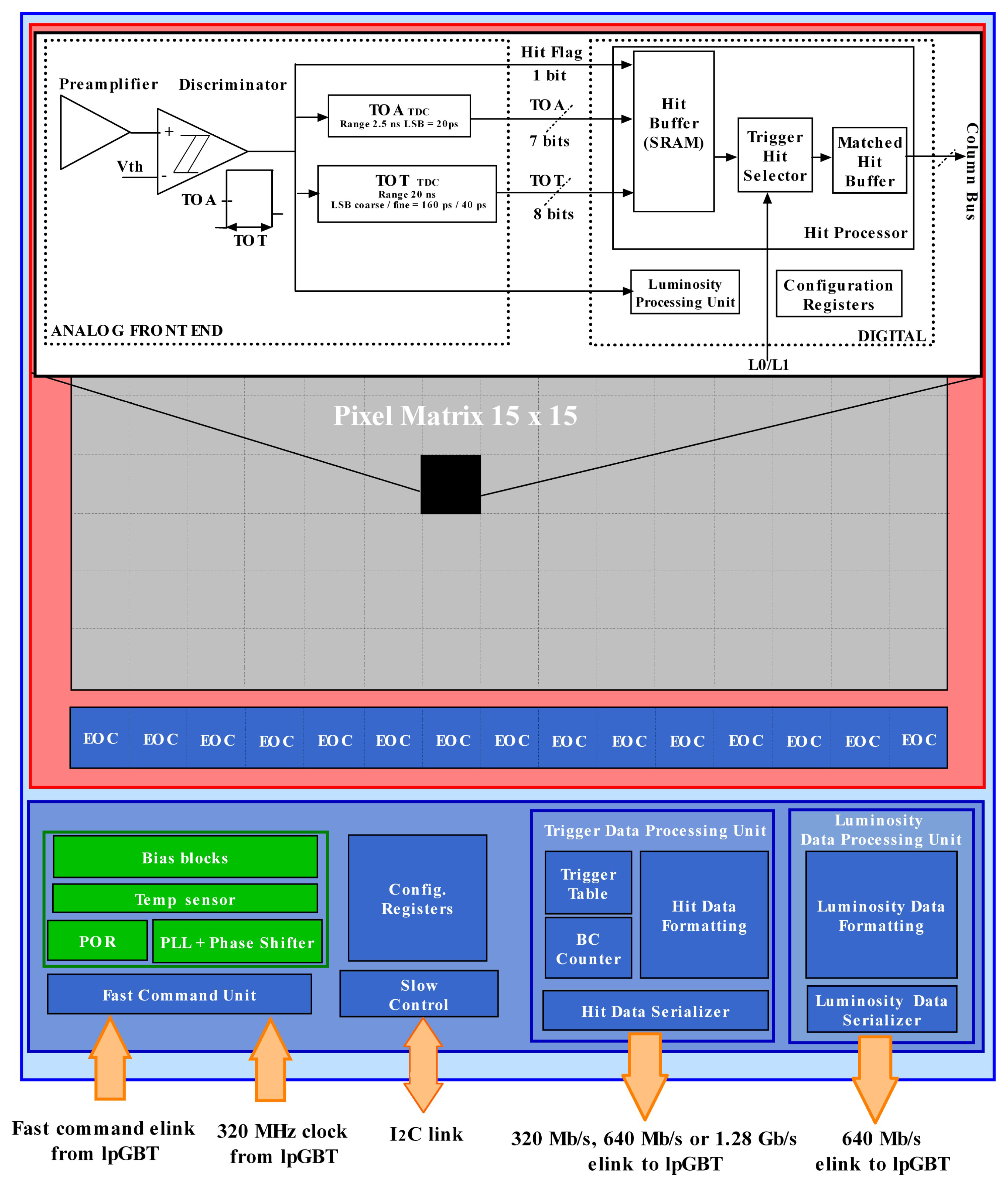
2. Front-End Readout System ASIC

The pixel frontend design (see Figure 1) consists of the analog and digital parts. The analog part incorporates a preamplifier followed by a discriminator and two TDCs, TOA TDC, and Time Over Threshold (TOT) TDC, which measure the Time of Arrival and the time over threshold of the signal. Each chip contains a matrix of 15 × 15 pixels of 1.3 mm × 1.3 mm.

One of the most important aspects to be understood is the TOA TDC performance. To characterize the TOA TDC, we can follow two different methodologies, both leading to similar results. The first one consists of injecting a signal at the input of the analog part of the ASIC, while in the second method we inject it directly at the input of the TDC just after the discriminator, avoiding the previous components. The last method is more accurate since it avoids all noise terms that can be added to the signal before reaching the TDC. The delay between two consecutive triggers is generated by the 40 MHz clock shifting. For each one, we compute the TOA and then fit the TOA vs. delay curve in order to extract the least significant bin (LSB), which is the the smallest measurable time window in ps, of the TOA TDC.

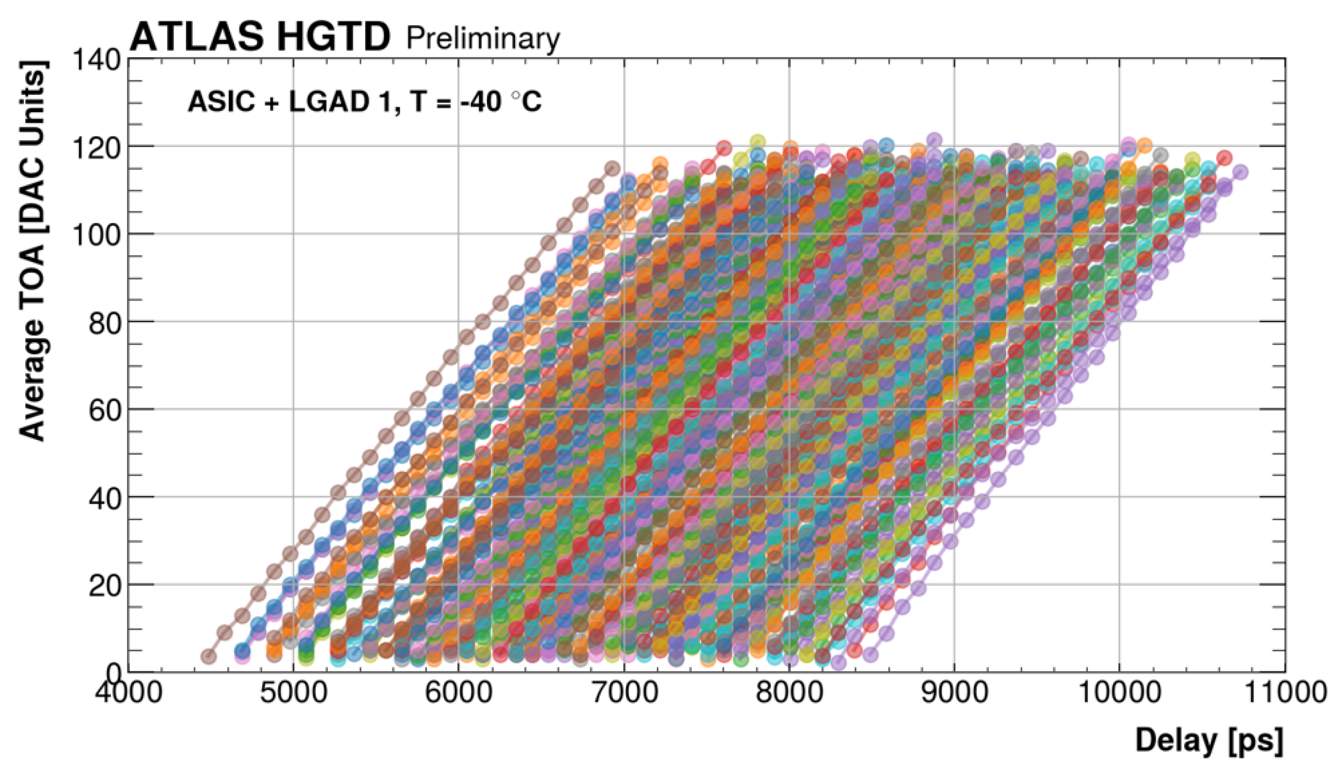
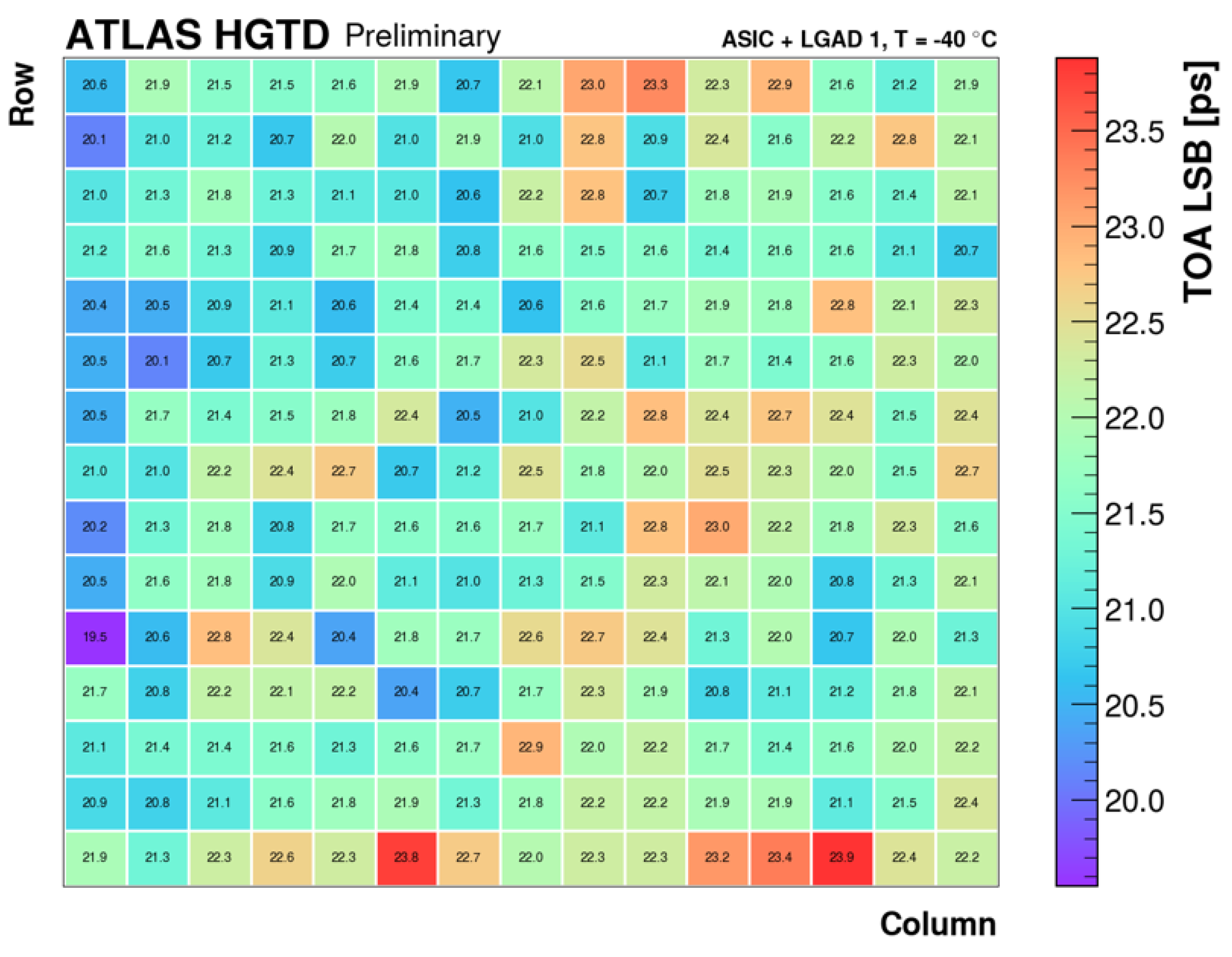
2.1. TOA TDC Calibration

Figure 2 shows the average TOA measurement with the TDC as a function of the programmable delay using direct injection of a digital pulse at the input of the TDCs. Each curve belongs to one single channel of the matrix. The temperature shown in the figure is that of the climate chamber, which was set to −40 °C in order to have the module temperature around −30 °C, which corresponds to the expected operation temperature in the experiment.

In order to compute the LSB, a linear regression is applied to extract the slope, thus LSB = 1/slope. Figure 3 shows the LSB map of one module (ASIC + LGAD sensor). We do not observe any clear dependency over columns nor over rows; also, we have reasonable homogeneity with RMS ≈ 0.7 ps, which is negligible compared to the average LSB, usually around 20 ps.

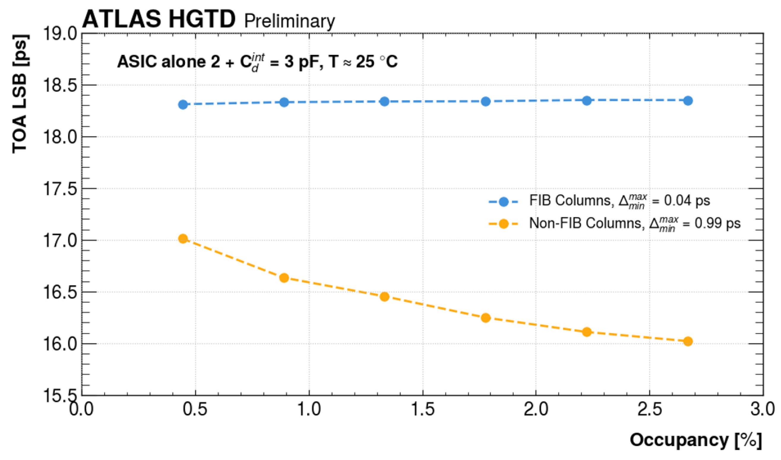
2.2. TOA LSB vs. Occupancy

One of the parameters that affect the value of the LSB is the number of injected pixels at once, i.e., the occupancy. To study this, we measure the TOA LSB of one specific pixel under different occupancy conditions and with different patterns of injection. We inject either using the:

• The column pattern, where we start by injecting in pixel i, then we keep adding pixels from the same column until we fill all of them, and then we move to the next column.
• The row pattern, where we start by injecting in pixel i, then we keep adding pixels from the same row until we fill all of them, and then we move to the next row.

During the HL-LHC phase, we expect at most an occupancy of around 10%, so the probability to have 15 hits within the same column or the same row is low [2]. However, since the shape of the ASIC chip is two-dimensional, by studying those patterns we can probe all the different phenomena that can degrade the performance of the chip. The impact of occupancy with the random pattern is small. We notice that even a very small variation of 0.1 ps in the LSB can lead to around 12.7 ps of variation if we integrate over the 127 TOA codes.

While with ALTIROC2 the voltage drop variation among the 15 columns was considered to be problematic, the ALTIROC3 design has been improved so that each pixel is powered separately using a specific bus to mitigate this issue, but the drop at the level of one column is still non-avoidable. This explains why we observe an increase below an occupancy of 7% (see Figure 4). No variation of LSB is expected using row-pattern injection. However, we see that the LSB decreases after this value of occupancy when we start adding pixels from another column. This effect has been understood as a parasitic effect due to an internal coupling between the On–Off voltage controlling the bin value of the TOA TDC and the TOA busy signal, which is a debugging signal.

To test this hypothesis, we used a Focused Ion Beam to cut the TOA busy signal from odd columns. Then, we started the test by injecting in pixel 0 followed by adding pixels either from even columns (Non-FIB ones) or pixel 15 followed by adding pixels from odd columns (FIB ones).

Figure 5 proves that for the FIB columns the variation is negligible since the coupling does not exist anymore, while for the Non-FIB ones we still observe the same effect. The TOA busy signal was therefore removed from the preproduction chip design (ALTIROCA).

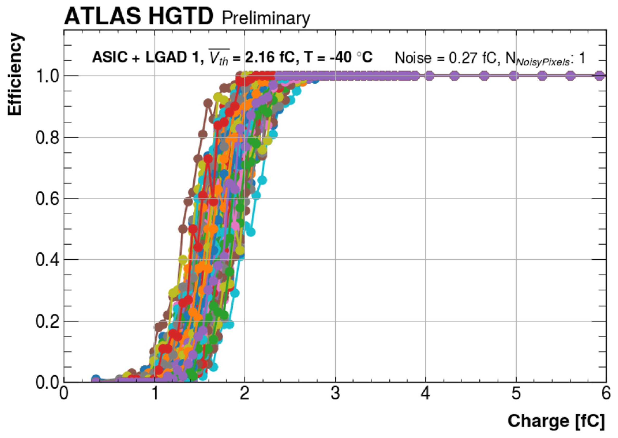
2.3. Minimal Detectable Charge

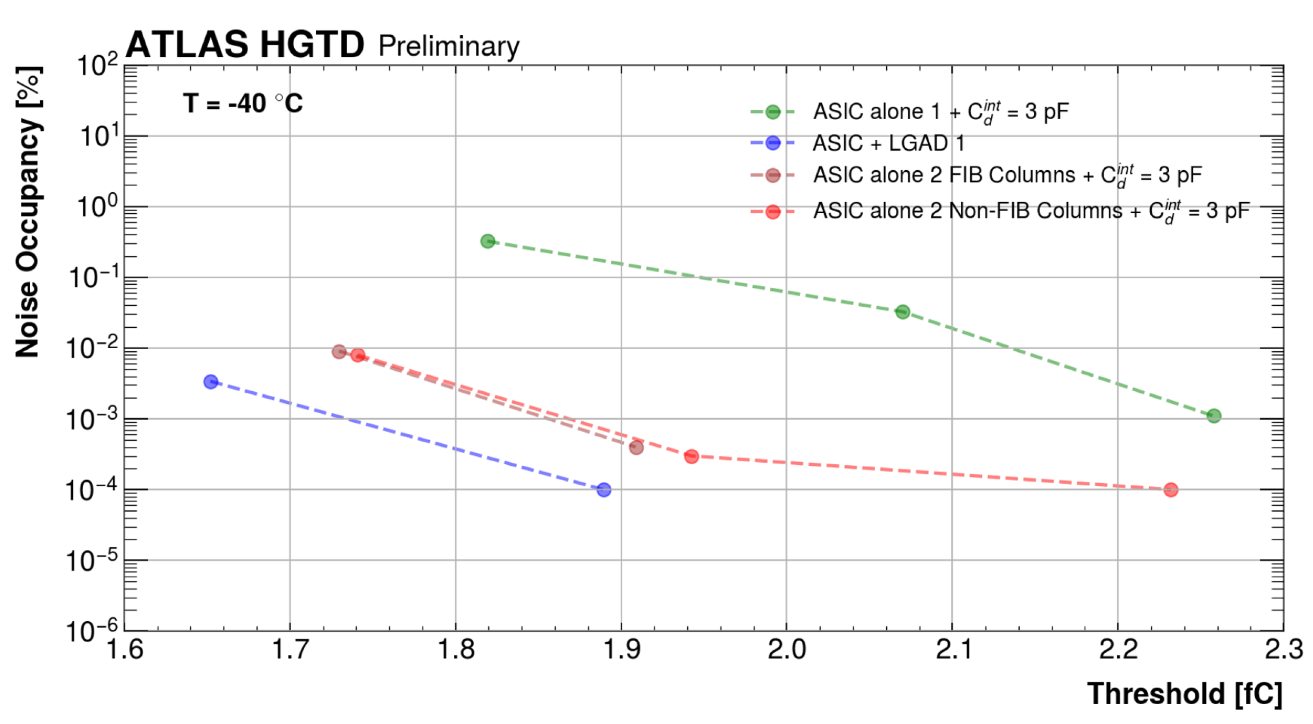
Accessing charge values down to 4 fC (1 fC equals 10⁻¹⁵C) is one of the main requirements. To achieve this goal, our readout system should be able to measure such low-charge values with good efficiency. Figure 6 shows the S-curve efficiency as a function of charge. The different curves belong to the 225 channels. On average with this board, we measure Q_min ≈ 2.2 fC. This value is consistent with the requirement.

2.4. Noise

The dark noise is an important factor because it is strongly coupled to the minimal detectable charge. In order to have clean and efficient measurements of small charge values, noise must be negligible for all threshold values greater than 4 fC. Figure 7 shows the dark noise percentage as a function of the threshold for four ALTIROC3 boards, obtained with random triggers for an acquisition window of 25 ns. The plot shows a negligible noise for all threshold values higher than 2.2 fC meeting the requirements.

2.5. Jitter

The jitter is one of the main contributors to the time-resolution, due to electronic noise. The specifications require jitter to be less than 25 ps for a charge of 10 fC. In Figure 8, the variation of jitter as function of the charge is shown for four boards. This measurement is carried out with a threshold of 4 fC. The jitter goes down quickly with increased charge, and it reaches 20 ps on average at 10 fC.

3. Test Beam Measurements

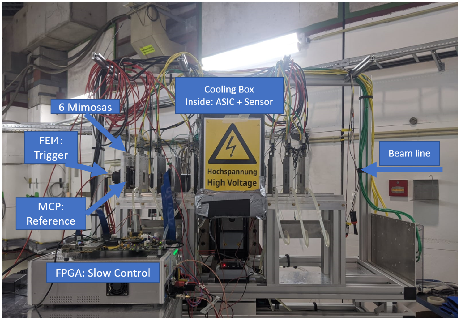
3.1. Setup

The test beam setup at DESY is shown in Figure 9. The beam of electrons with 3.5–5 GeV momentum comes from the right to left part of the figure. The trigger logic was handled by a programmable Trigger Logic Unit TLU [4]. Six MIMOSA [5] pixel planes with an approximate tracking spatial resolution of ${\sigma }_{\mathrm{xy}}\approx$ 20 µm were used for the track reconstruction. The digitized data of ALTIROC3 are transmitted through the FPGA to a control PC, while the full waveforms of the 40 MHz clock, the MCP [6], which is a timing reference detector with negligible time-resolution of around 10 ps compared to the ASIC’s one, and the analogue ASIC probe are sampled by a Lecroy oscilloscope. This FPGA is also used for ALTIROC configuration. The ASIC probe can be used to do time-walk correction by directly using the charge information at the output of the preamplifier instead of the TOT. The cooling box is key part of the setup since it helps to control the temperature of the module. The noise term is affected by the temperature, so by lowering the temperature we reduce the thermal noise and improve the precision of the measured signals. The selection of synchronized events, which simultaneously cross both the Module and the MCP, is carried out using a FEI4 [7] readout chip with a small adjustable region-of-interest trigger output.

A similar setup has been used for test-beam campaigns at the CERN SPS H6 beam line, operated with pions of 120 GeV momentum. So far, five test beam campaigns, at DESY and CERN, have been conducted between November 2023 and August 2024.

We define the time-resolution as the standard deviation of the Gaussian fit of the distribution of the reference time subtracted from the ASIC time. This distribution is given by the following formula:

$$\Delta (\mathrm{TOA},{\mathrm{T}}_{\mathrm{ref}})=-\mathrm{LSB}\times \mathrm{TOA}-({\mathrm{T}}_{\mathrm{CLK}}-{\mathrm{T}}_{\mathrm{MCP}}),$$

where:

• LSB is the least significant bit of the chosen pixel.
• TOA is the Time of Arrival.
• ${\mathrm{T}}_{\mathrm{CLK}}$ is the front end time of the 40 MHz clock signal.
• ${\mathrm{T}}_{\mathrm{MCP}}$ is the time of the MCP signal.

The computation of the LSB can be carried out inclusively or exclusively. With the first method, we fit the full TOA vs. delay curve as shown in Figure 2. Using the latter method, we multiply each LSB by the corresponding TOA distribution cycle, where each cycle is contains 32 codes. Since the TOA codes vary between 0 and 127, we have four cycles leading to four LSBs, before merging all of them. In the following section, we show the measurements performed with 120 GeV charged pions at the CERN SPS H6 beam line in May 2024. The temperature inside the cooling box was set at −38.5 °C. Under this condition, the temperature of the module is around −30 °C. The sensor is a ATLAS-HGTD preproduction sensor of IHEP-IME design with a breakdown voltage ${\mathrm{V}}_{\mathrm{bd}}$∼ 170 V at room temperature (V1-R5 17—ID: 20WS1001000517).

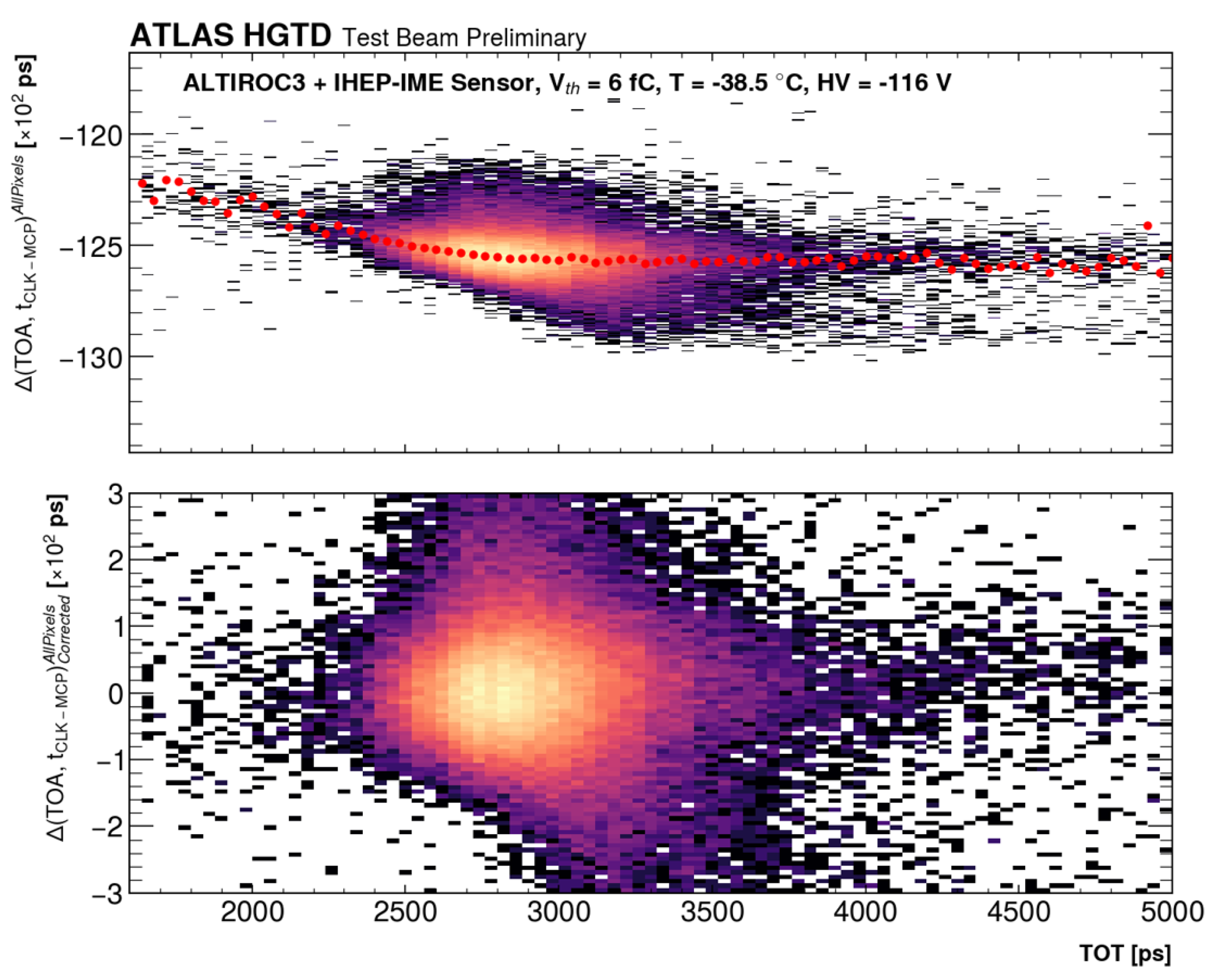
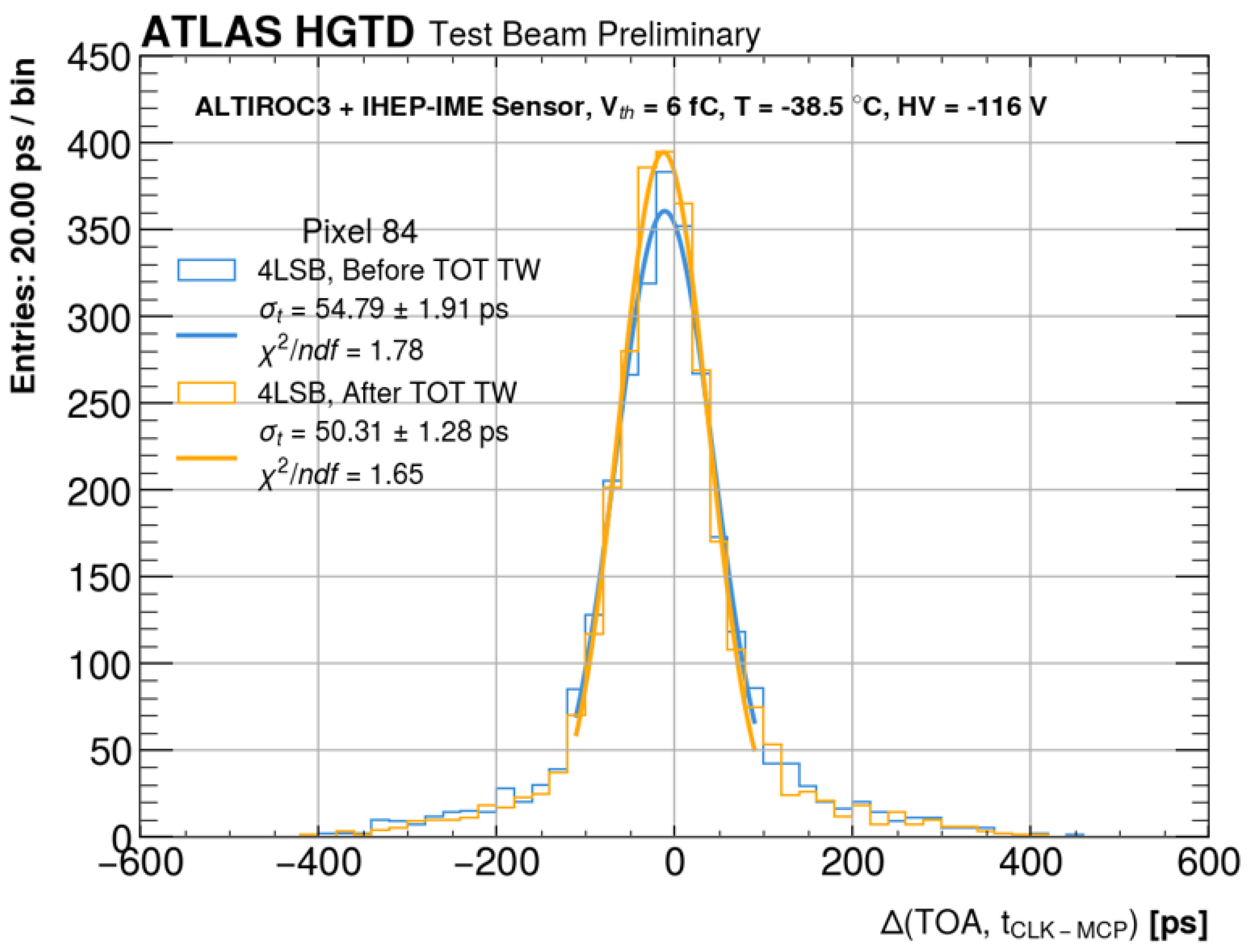
3.2. Time-Walk Correction

The Time of Arrival depends on the collected charge. The time-walk effect [8] is caused by the fact that, for a constant rise time, a signal with a smaller amplitude will cross the threshold later than a signal with a higher amplitude, introducing a shift on the TOA measurement. The contribution to the time-resolution is given by ${\left[{\displaystyle \frac{{\mathrm{V}}_{\mathrm{th}}}{\mathrm{S}/{\mathrm{t}}_{\mathrm{rise}}}}\right]}_{\mathrm{RMS}}$, where V_th is the threshold amplitude, S is the signal amplitude, and t_rise is the rise time. In the case of measuring the signals with a Constant Threshold Discriminator (CTD), the presence of this noise is unavoidable. A correction can be made using different methods like Time Over Threshold (TOT), which is ideally proportional to the collected charge. To achieve accurate timing measurements, this dependency between TOA and collected charge is removed, which is an essential process known as time-walk correction.

The correction procedure involves the following steps: first, the TOT range is divided into bins of 40 ps each. Then, for each TOT bin, we combine all tested channels distributions of the TOA difference between the hybrid module and a MCP + 40 MHz clock reference system. Next, the full $\Delta (\mathrm{TOA},{\mathrm{T}}_{\mathrm{ref}})$ is fit with a Gaussian function. Therefore, the mean of this Gaussian fit represents the systematic shift due to the time-walk effect for that particular TOT bin. Finally, this mean value is subtracted from the TOA to correct for the time-walk effect. The residuals after subtraction represent the corrected $\Delta (\mathrm{TOA},{\mathrm{T}}_{\mathrm{ref}})$ distribution, which should be independent of the collected charge in case of ideal correction.

In the top plot of Figure 10, we show the $\Delta (\mathrm{TOA},{\mathrm{T}}_{\mathrm{ref}})$ distribution of all pixels combined as a function of the TOT measured by the ASIC. The red dots correspond to the mean values of each TOT bin $\Delta (\mathrm{TOA},{\mathrm{T}}_{\mathrm{ref}})$ distributions. In the bottom plot, we show the corrected distribution obtained by subtracting the mean values. Even though the corrected distribution is centered around 0, dedicated studies showed that the TOT variable is not perfectly linear with the charge due to various issues, so a specific correction made using the probed charge distribution instead of the TOT one shows that the residual time-walk contribution after TOT time-walk correction is around 25 ps on average.

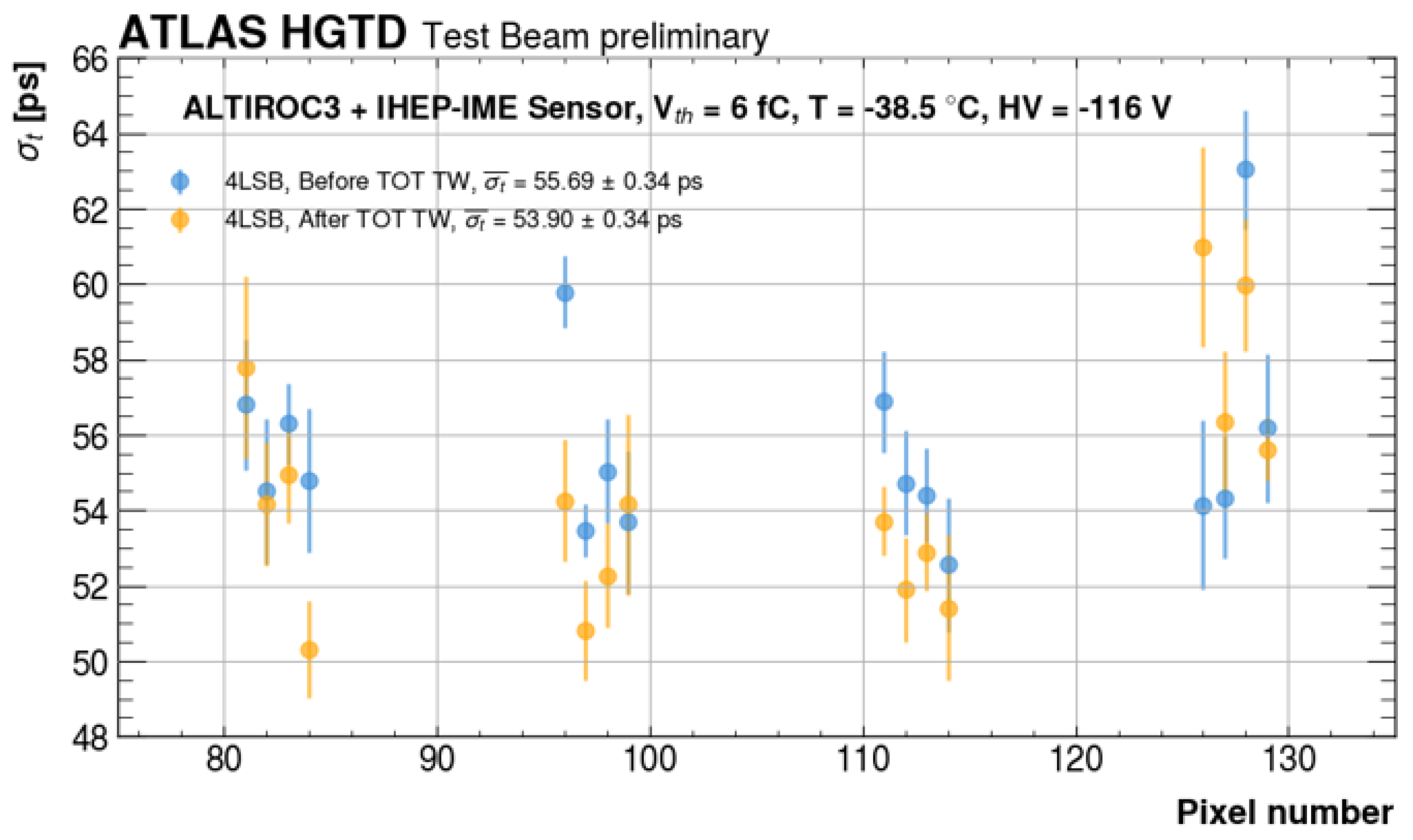
3.3. Time-Resolution

In Figure 11, we show the $\Delta (\mathrm{TOA},{\mathrm{T}}_{\mathrm{ref}})$ distribution of pixel 84 before and after time-walk correction. We notice the presence of the non-Gaussian tail in the distribution. This tail can result from multiple factors. The measured jitter for 6 fC charge particle using a threshold of 5 fC is around 40 ps. This value will increase significantly when the charge value is very close to the settled threshold. More dedicated studies are needed to understand the origin of the tail. As shown by Figure 8 for this pixel, the time-resolution is 54.8 ps before correction, while it is 50.3 ps after correction. Figure 12 shows the time-resolution for multiple tested pixels. The average value is 53 ps after time-walk correction.

4. Summary

To conclude, we have studied the timing performance of the ALTIROC using a test bench and during test beam campaigns. ALTIROC shows good performance in terms of jitter, efficiency, and charge collection, meeting the requirements of the HL-LHC phase. Some effects like inconsistency between calibration LSB and test beam data, LSB non-linearity, and the dependency of LSB on occupancy are being further studied. We also give an overview of the test beam campaign results. On average, the time resolution we have obtained is around 50 to 55 ps. This value can vary depending on the board, the threshold, the high voltage value applied, and many other factors. More aspects like refining time-walk correction and non-Gaussianity effects can be further investigated in the future.

References

1. ATLAS Collaboration. The ATLAS Experiment at the CERN Large Hadron Collider. JINST 3 (2008) S08003. Available online: https://iopscience.iop.org/article/10.1088/1748-0221/3/08/S08003 (accessed on 1 June 2023).
2. ATLAS Collaboration. Technical Design Report: A high Granularity Timing Detector for the ATLAS Phase-II Upgrade. Tech. Rep. CERN-LHCC-2020-007, ATLAS-TDR-031, CERN, Geneva. 2020. Available online: https://cds.cern.ch/record/2719855?ln=en (accessed on 1 May 2023).
3. Sadrozinski, H.F.W.; Seiden, A.; Cartiglia, N. 4-Dimensional Tracking with Ultra-Fast Silicon Detectors. Rept. Prog. Phys. 2018, 81, 026101. [Google Scholar] [CrossRef] [PubMed]
4. Description of the Jra1 Trigger Logic Unit (tlu), v0.2c. Tech. Rep. 2009. Available online: http://www.eudet.org/e26/e28/e42441/e57298/EUDET-MEMO-2009-04.pdf (accessed on 1 January 2024).
5. Jansen, H.; Spannagel, S.; Behr, J.; Bulgheroni, A.; Claus, G.; Corrin, E.; Cussans, D.; Dreyling-Eschweiler, J.; Eckstein, D.; Eichhorn, T.; et al. Performance of the EUDET-type beam telescopes. EPJ Tech. Instrum. 2016, 3, 7. [Google Scholar] [CrossRef]
6. Ronzhin, A.; Los, S.; Ramberg, E.; Apresyan, A.; Xie, S.; Spiropulu, M.; Kim, H. Study of the timing performance of micro-channel plate photomultiplier for use as an active layer in a shower maximum detector. Nucl. Instrum. Methods A 2015, 795, 288–292. [Google Scholar] [CrossRef]
7. Albert, J.; Alex, M.; Alimonti, G.; Allport, P.; Altenheiner, S.; Ancu, L.S.; Andreazza, A.; Arguin, J.; Arutinov, D.; Backhaus, M.; et al. Prototype ATLAS IBL Modules using the FE-I4A Front-End Readout Chip. J. Instrum. 2012, 7, P11010. [Google Scholar]
8. Leo, W.R. Techniques for Nuclear and Particle Physics Experiments, 2nd ed.; Springer: Berlin, Germany, 1994; ISBN 0-387-57280-5. [Google Scholar]
Figure 1. Front end readout system design [2].
Particles 08 00050 g001
Figure 2. Variation of TOA as function of the delay for ALTIROC3 hybrid.
Particles 08 00050 g002
Figure 3. TOA LSB map for ALTIROC3 hybrid.
Particles 08 00050 g003
Figure 4. Column vs. row patterns of injection variation of LSB as function of the occupancy for ALTIROC3 ASIC alone.
Particles 08 00050 g004
Figure 5. FIB vs. Non-FIB column variation of LSB as function of the occupancy when injecting with row pattern for ALTIROC3 ASIC alone.
Particles 08 00050 g005
Figure 6. Efficiency as function of the charge for ALTIROC3 hybrid. We apply a sigmoid fit to extract the threshold, which is defined as the charge value for which the efficiency reaches 95%. The average threshold over all pixels is around 2.16 fC.
Particles 08 00050 g006
Figure 7. Noise occupancy as function of threshold for the ALTIROC3 hybrid.
Particles 08 00050 g007
Figure 8. Jitter as function of the injected charge for ALTIROC3 hybrid.
Particles 08 00050 g008
Figure 9. Test beam setup at DESY beamline.
Particles 08 00050 g009
Figure 10. Time-walk correction. On the top plot we show Δ ( TOA , T ref ) distribution as function of TOT before time-walk correction. In the bottom one, we show it after time-walk correction.
Particles 08 00050 g010
Figure 11. Time-resolution before (blue) and after (orange) time-walk correction for a single pixel. To extract the time resolution, we fit the full distribution with a Gaussian. Then, we use the extracted mean and sigma values to fit the core of the distribution with a second Gaussian starting from the previous extracted values as initial guess.
Particles 08 00050 g011
Figure 12. Time-resolution before (blue) and after (orange) time-walk correction for all tested pixels.
Particles 08 00050 g012
Disclaimer/Publisher’s Note: The statements, opinions and data contained in all publications are solely those of the individual author(s) and contributor(s) and not of MDPI and/or the editor(s). MDPI and/or the editor(s) disclaim responsibility for any injury to people or property resulting from any ideas, methods, instructions or products referred to in the content.