Information Field Theory for Two Applications in Astroparticle Physics

Abstract

Information field theory (IFT) provides a powerful framework for reconstructing continuous fields from noisy and sparse data. Based on Bayesian statistics, IFT allows for the approximation of posterior distributions over field-like parameter spaces in high-dimensional problems. In this contribution, we discuss two applications of IFT in the context of astroparticle physics. First, we present its intended use for the calibration of the newly installed radio detector upgrade of the Pierre Auger Observatory. Second, we demonstrate its application to infer the initial directions of ultra-high-energy cosmic rays before their deflection in the Galactic magnetic field using a simplified model.

1. Introduction

The study of ultra-high-energy cosmic rays (UHECRs) is a key research area in astroparticle physics. UHECRs are believed to be charged nuclei with energies exceeding ${10}^{18}\mathrm{eV}$. The detection of UHECRs in cosmic ray observatories provides valuable information, which can be used to learn about the characteristics of their sources and acceleration mechanism. When UHECRs arrive at Earth, they interact with air molecules and initiate air showers of secondary particles. The detection of these air showers is challenging due to the low UHECR flux of about one particle per square kilometer per century. Extracting meaningful information from UHECR data is complicated not only by this statistical sparsity but also by measurement uncertainties and the high dimensionality of the data, encompassing energy, arrival direction, and shower depth. Additionally, the deflection of UHECRs in the Galactic magnetic field (GMF) hinders the identification of their sources [1].

Given these challenges, analyzing the sparse and noisy data requires solving high-dimensional inference problems, which information field theory (IFT) is particularly well-suited for [2]. Traditional methods for data reconstruction often rely on simpler statistical models or interpolation techniques that may fail to account for prior physical knowledge or struggle with high-dimensional spaces. In contrast, IFT employs Bayesian statistics to incorporate prior information and provides a robust framework for approximating posterior distributions over complex parameter spaces. This capability makes IFT a powerful tool for solving Bayesian problems with the straightforward integration of experimental uncertainties and prior knowledge.

The application of IFT in astrophysics has been successfully demonstrated in various studies, such as Bayesian radio interferometry [3] or the reconstruction of the spatial distribution of gas in the Milky Way [4]. This study explores the application of IFT to two problems in astroparticle physics. First, we demonstrate its application in the calibration of radio antennas for the detection of extensive air showers induced by UHECRs. The calibration of the antennas is crucial for the reconstruction of the electric field of the radio signals emitted by the air showers, which is essential for the reconstruction of the air shower geometry and the energy of the primary cosmic ray. Second, we show how IFT can be used to infer the initial flux distribution of UHECRs before their deflection in the GMF.

2. Information Field Theory

IFT [2] is a statistical framework for the reconstruction of continuous fields from noisy and sparse data. It is based on Bayesian statistics and allows for the approximation of posterior distributions over field-like parameter spaces in high-dimensional problems. Prior information that contains physical knowledge about the problem at hand can be naturally incorporated into the reconstruction process to confine the solution to physically meaningful regions of the parameter space. The uncertainties of the parameters of interest are naturally reflected in the posterior distribution, which allows for a rigorous treatment of the physical uncertainties in the reconstruction.

The measurement equation

$$d=R\left[s\right]+n$$

(1)

relates the data d to the field s through the response operator R, which describes the physical process that maps the field to the data. s is the field of interest, which can be a scalar or vector field defined on a continuous domain. This field can represent, for example, the temperature in a room, the electric field of a radio signal, or the flux of UHECRs. The noise n corresponds to statistical uncertainties in the data.

Inference using Bayesian statistics involves relating a likelihood function together with prior information to the posterior distribution in question. The prior information is contained in the prior distribution $P\left(s\right)$ and can be chosen to reflect the expected physical properties of the field, such as smoothness or spatial correlations. The latter are encoded in the power spectrum of the field. Specific hyperparameters can be used to model the power spectrum of the field, such as the double-logarithmic average slope, asperity, flexibility, fluctuations, and offset [5]. The double-logarithmic average slope describes the overall behavior of the power spectrum, while the asperity and flexibility characterize the behavior of the integrated Wiener process. The fluctuations determine the overall amplitude of the field, while the offset adds a constant to the field realizations. The effects of these hyperparameters on the field are demonstrated in [6]. Except for the double-logarithmic average slope, which is modeled using a normal distribution, the hyperparameters are modeled with log-normal distributions. As IFT makes minimal assumptions about the underlying field, we refer to it as the non-parametric correlated field.

The goal of IFT is to infer the posterior distribution $P\left(s\right|d)$ of the field given the data. To this end, the software package NIFTy [7] provides inference algorithms, such as geometric variational inference [8], that allow for the efficient approximation of the posterior distribution. Variational inference approximates the posterior distribution by minimizing the Kullback–Leibler divergence [9] between the true posterior and the predicted distribution. This allows for the efficient computation of the posterior distribution and the estimation of uncertainties in the field reconstruction. The non-parametric correlated field model in NIFTy allows for the incorporation of prior information about the field via the hyperparameters of the power spectrum.

NIFTy has been updated using the machine learning framework JAX [10] to enable the use of modern programming features. These include automatic differentiation, which is crucial for the implementation of variational inference algorithms. Just-in-time compilation, the use of NVIDIA’s CUDA backend [11], and the possibility to easily parallelize functions over arrays with the vmap function are further advantages of JAX speeding up the computation of the posterior distribution.

In this work, the following software versions were used: NIFTy 8.5.2, JAX 0.4.30, jaxlib 0.4.30, and ducc0 0.35.0.

3. Drone-Based Calibration of Radio Antennas

Radio detection of UHECRs is a promising method to study the most energetic particles in the universe [12]. When UHECRs reach Earth, they interact with the atmosphere and produce extensive air showers, which emit radio signals that can be detected by radio antennas. The geomagnetic effect arises from the deflection of electrons and positrons in the Earth’s magnetic field, generating a time-varying current and emitting radio waves [13]. The Askaryan effect contributes additional radio emission due to a charge excess when electrons and ions separate with their different velocities along the shower [14]. The radio signals are detected by antennas, which are used to reconstruct the air shower geometry and the energy of the primary cosmic ray.

Short aperiodic loaded loop antennas (SALLAs) have recently been deployed as part of the Auger Prime upgrade of the Pierre Auger Observatory [15]. In addition to simulation studies, the calibration of these antennas is crucial to understand the antenna response to the radio signals emitted by the air showers. While the absolute calibration of the antennas can be performed by using the Galactic radio background, the directional calibration can be performed by emitting a signal from a known location and measuring the response of the antennas. For this purpose, a drone is used to carry a transmitter that emits a reference signal at a known frequency. The drone is flown in a dome-like pattern above the antenna, and the antenna measures the signal emitted by the drone. The data recorded by the antenna can then be used for the calibration.

The directional dependence of the antennas can be described by the vector effective length (VEL) $\overrightarrow{\mathcal{H}}$. The VEL relates the voltage $\mathcal{U}$ measured by the antennas to the electric field $\overrightarrow{\mathcal{E}}$ of the incoming signal. In the frequency domain, this relates to

$$\mathcal{U}(\varphi ,\theta ,f)=\overrightarrow{\mathcal{H}}(\varphi ,\theta ,f)·\overrightarrow{\mathcal{E}}\left(f\right),$$

(2)

where $\varphi$ and $\theta$ are the azimuthal and polar angles, respectively. The VEL can be interpreted as a vector field that describes the directional dependence of the antennas. The calibration of the antennas aims to infer the VEL from the signal emitted by the drone and the voltage measured by the antenna.

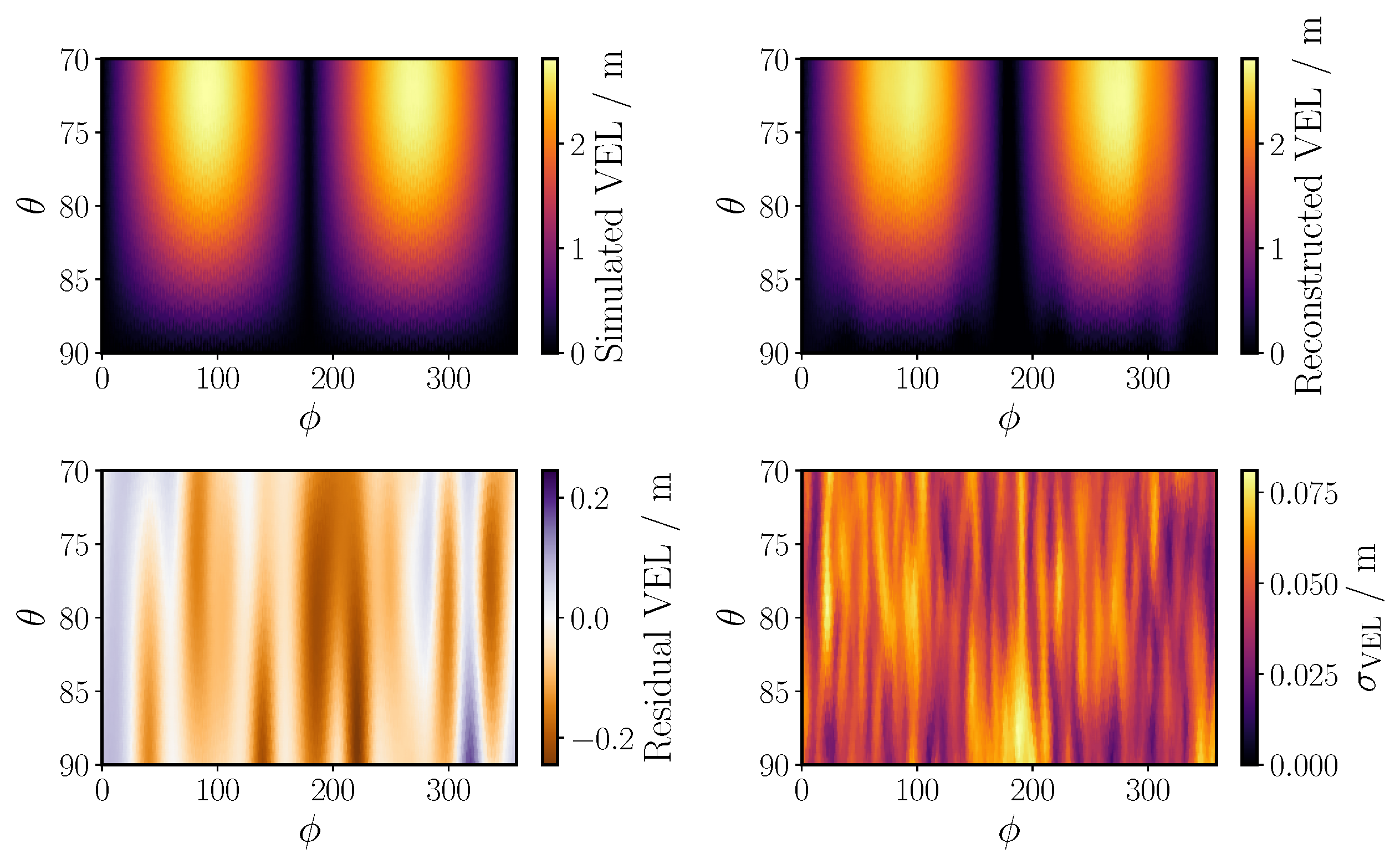
A mock data set resembling a real-world calibration scenario was generated using a simulated VEL. The VEL was simulated using the NEC-2 software [16]. The mock data set resembles the power that would be recorded by the antennas during a calibration flight. The total number of data points is 102. The detailed simulation setup can be found in [17]. The mock data set was then used to infer the VEL using IFT. Prior information about the VEL was incorporated into the reconstruction using the correlated field model. The hyperparameters of the correlated field model are shown in

Table 1. Hyperparameters used for the correlated field model in the VEL reconstruction. The double-logarithmic average slope is modeled as a normal distribution, while the other hyperparameters are modeled as log-normal distributions. The angular hyperparameters describe the VEL in the azimuthal and polar angles, while the spectral hyperparameters describe the VEL in the frequency domain.

Hyperparameter	$\mathsf{\mu }$	$\mathit{\sigma }$
Angular fluctuations	0.5	0.5
Angular double-logarithmic average slope	−4.0	0.1
Angular flexibility	0.2	0.02
Angular asperity	0.01	0.0014
Spectral fluctuations	0.5	0.1
Spectral double-logarithmic average slope	−4.0	2.0
Spectral flexibility	2.0	0.2
Spectral asperity	0.01	0.5

. These hyperparameters were optimized to reflect the expected properties of the VEL. Two exemplary slices of $\theta$ and $\varphi$ at a frequency of $f=55\mathrm{MHz}$ are shown in Figure 1. The mock data, the underlying truth of the VEL, and the reconstruction mean with the respective 1$\sigma$ band are presented. It is visible that the IFT reconstruction of the VEL is in good agreement with the underlying truth for these specific slices. This is also true for the full VEL, which is shown in Figure 2. The simulated truth, the reconstruction mean, the residual, and the reconstructed standard deviation are shown. The results show agreement between the mock data and the reconstruction. The reconstructed mean is in agreement with the simulated truth. The predicted uncertainties indicate a high precision of the reconstruction, which is crucial for small overall uncertainties in the calibration of the antennas. For this realistic simulation setup, an uncertainty of a few percent is achieved, which is sufficient for the analysis of the radio signals emitted by air showers where the aim is to achieve an overall uncertainty of around $10\%$. This example reconstruction achieves a reduced chi-squared value of ${\chi }^2/n_{\mathrm{dof}}=1.7$, indicating consistency between the mock data and the prediction. The frequency dependence is not shown here but is also precisely reconstructed [17].

Current work focuses on the application of this calibration method to real data recorded by the Pierre Auger Observatory [18].

4. Inferring the Ultra-High-Energy Cosmic Ray Flux Prior to Deflection in the Galactic Magnetic Field

The sources and acceleration mechanisms of UHECRs are still largely unknown. The observation of a dipole in the arrival directions of UHECRs [19] suggests an extragalactic origin. However, deflection in the GMF complicates the identification of their sources, as the observed arrival directions generally do not point back to the origin of the UHECRs.

The GMF is typically modeled as a combination of a regular and a turbulent component, with field strengths of a few $\mathsf{\mu }\mathrm{G}$. For this study, we chose to use the base model of the Unger–Farrar (UF23) GMF models [20] as the regular component, while neglecting the turbulent component for simplicity. The UF23 models are state-of-the-art GMF models that are based on observational data while providing a detailed description of the GMF structure. The regular component of the GMF models includes contributions from a large-scale halo field and a logarithmic spiral field, which are modeled using analytical functions. The UF23 models have been shown to reproduce the observed Faraday rotation measures and synchrotron emission, making them a suitable choice for this study. The variety of UF23 models allows for an uncertainty estimate in the theoretical modeling, which can be included in future work.

The deflection of UHECRs in the GMF depends on their rigidity, $R=E/Z$, where E is the energy and Z the charge of the particle. In our model, we assume the UHECRs are purely protons with an energy of ${10}^{19.2}\mathrm{eV}$.

To simulate the deflection, a GMF lens is constructed by propagating anti-particles from Earth to the edge of the Galaxy. This backtracking method has the advantage that every simulated trajectory is observed at Earth. The lens is constructed for a given rigidity and is used to propagate the extragalactic illumination map of UHECRs to the sky map at Earth. The extragalactic illumination map describes the flux of UHECRs before their deflection in the GMF. The sky map at Earth describes the observed flux of UHECRs. Mathematically, the GMF lens relates the extragalactic illumination map $\overrightarrow{b}$ to the observed sky map at Earth $\overrightarrow{a}$ via

$$\overrightarrow{a}=L\overrightarrow{b},$$

(3)

where L is the GMF lens matrix that encodes the deflection direction and strength of the GMF for the given rigidity. The goal is to infer the extragalactic illumination map $\overrightarrow{b}$ from the measured sky map $\overrightarrow{a}$.

To this end, we use a forward model that describes the deflection of UHECRs in the GMF. The forward model uses the GMF lens to propagate the extragalactic illumination map to the sky map at Earth. Afterwards, the sky map is convolved following the exposure of the Pierre Auger Observatory to obtain an expected measured flux.

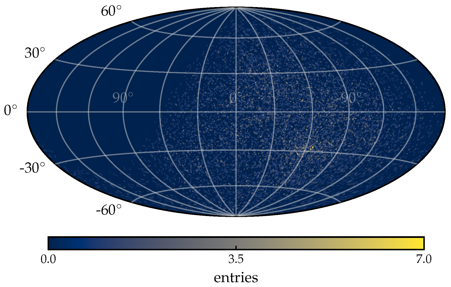
The forward model was used to calculate an exemplary probability distribution for the number of measured UHECRs at Earth per pixel in a HEALpix [21] grid with $N_{\mathrm{side}}=64$. This probability distribution was then used to generate a mock data set by drawing the number of measured UHECRs per pixel from a Poisson distribution. This resembles the data that would be recorded by the Pierre Auger Observatory [22] and is shown in Figure 3. The mock data set was used to infer the extragalactic illumination map using IFT. The hyperparameters of the correlated field model used for the reconstruction are shown in

Table 2. Hyperparameters used for the correlated field model in the extragalactic illumination map reconstruction. The double-logarithmic average slope is modeled as a normal distribution, while the other hyperparameters are modeled as log-normal distributions. The hyperparameters describe the power spectrum of the extragalactic illumination map.

Hyperparameter	$\mathsf{\mu }$	$\mathit{\sigma }$
Fluctuations	0.4	0.05
Double-logarithmic average slope	−2.0	0.01
Flexibility	1.0	0.5
Asperity	0.5	0.05

. The hyperparameters were optimized to reflect the expected properties of the extragalactic illumination map. To ensure the non-negativity of the extragalactic illumination map, the drawn field realizations are subjected to an exponential function prior to the inference.

For a HEALpix binning of $N_{\mathrm{side}}=64$, the extragalactic illumination map has $49,152$ pixels. While the forward process from the field to the data is fully determined except for statistical fluctuations, the high dimensionality of the problem makes traditional Bayesian methods infeasible. In contrast, IFT efficiently navigates this high-dimensional parameter space. This initial investigation of reconstructing the extragalactic illumination map using IFT focuses on addressing statistical fluctuations in the data. Future work will account for uncertainties arising from the collection of different GMF models, where IFT’s ability to incorporate prior information and handle uncertainties will be essential.

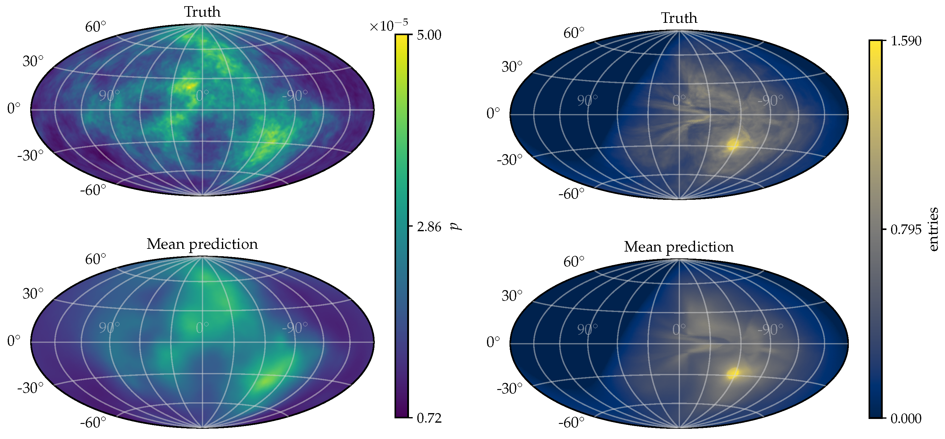
The mean reconstruction results for the mock data are shown in Figure 4. Both the extragalactic illumination map and the measured sky map at Earth are reconstructed with high precision. The reconstructed uncertainty and the relative difference between the truth and the reconstruction mean for the extragalactic illumination map are shown in Figure 5. The high uncertainty in the upper left of the extragalactic illumination map can be explained by the moderate exposure owing to the observatories location chosen to be on the Southern hemisphere. These results show that the reconstruction is consistent with the underlying truth of the mock data and allows for straightforward estimation of uncertainties.

Future work will focus on incorporating a more realistic composition and energy spectrum of UHECRs in the model. The systematic uncertainty arising from our limited knowledge of the GMF will be included in the model by using various UF23 models as GMF. This will help to better understand the deflection patterns and improve the accuracy of the inferred extragalactic illumination map.

5. Summary

In this work, we have presented two applications of IFT in the context of astroparticle physics. By employing Bayesian methods and advanced computational tools, IFT enables the reconstruction of complex, high-dimensional fields from sparse and noisy data.

First, we applied IFT to the directional calibration of radio antennas used at the Pierre Auger Observatory. The precise reconstruction results of the mock data show that IFT is a powerful tool for calibration tasks, where usually only sparse data are available. The calibration of the antennas is crucial for the reconstruction of the electric field of the radio signals emitted by air showers, which is essential for, e.g., the reconstruction of the air shower geometry and the energy of the primary cosmic ray.

Second, we demonstrated the application of IFT to infer the extragalactic illumination map of UHECRs before their deflection in the GMF. The reconstruction results for the simplified model show that IFT has the potential to infer the extragalactic flux of UHECRs from the observed sky map at Earth. Future work will incorporate a more realistic composition and energy spectrum of UHECRs, along with systematic uncertainties arising from limited GMF knowledge.

References

Farrar, G.R.; Sutherland, M.S. Deflections of UHECRs in the Galactic magnetic field. J. Cosmol. Astropart. Phys.2019, 2019, 004. [Google Scholar]
Enßlin, T.A. Information Theory for Fields. Ann. Phys.2019, 531, 1800127. [Google Scholar] [CrossRef]
Söding, L.; Edenhofer, G.; Enßlin, T.A.; Frank, P.; Kissmann, R.; Phan, V.H.M.; Ramírez, A.; Zandinejad, H.; Mertsch, P. Spatially coherent 3D distributions of HI and CO in the Milky Way. Astron. Astrophys.2025, 693, A139. [Google Scholar] [CrossRef]
Arras, P.; Frank, P.; Haim, P.; Knollmüller, J.; Leike, R.; Reinecke, M.; Enßlin, T. Variable structures in M87* from space, time and frequency resolved interferometry. Nat. Astron.2022, 6, 259–269. [Google Scholar] [CrossRef]
Edenhofer, G.; Frank, P.; Roth, J.; Leike, R.H.; Guerdi, M.; Scheel-Platz, L.I.; Guardiani, M.; Eberle, V.; Westerkamp, M.; Enßlin, T.A. Re-Envisioning Numerical Information Field Theory (NIFTy.re): A Library for Gaussian Processes and Variational Inference. J. Open Source Softw.2024, 9, 6593. [Google Scholar]
Huege, T. Radio detection of cosmic ray air showers in the digital era. Phys. Rep.2016, 620, 1–52. [Google Scholar]
Falcke, H.; Apel, W.D.; Badea, A.F.; Bähren, L.; Bekk, K.; Bercuci, A.; Bertaina, M.; Biermann, P.L.; Blümer, J.; Bozdog, H.; et al. Detection and imaging of atmospheric radio flashes from cosmic ray air showers. Nature2005, 435, 313–316. [Google Scholar] [CrossRef] [PubMed]
Askar’yan, G.A. Excess negative charge of an electron-photon shower and its coherent radio emission. Zh. Eksp. Teor. Fiz.1961, 41, 616–618. [Google Scholar]
The Pierre Auger Collaboration. Status and expected performance of the AugerPrime Radio Detector. PoS Proc. Sci.2023, ICRC2023, 344. [Google Scholar]
Ishii, M.; Baba, Y. Advanced computational methods in lightning performance. The Numerical Electromagnetics Code (NEC-2). In Proceedings of the 2000 IEEE Power Engineering Society Winter Meeting. Conference Proceedings (Cat. No.00CH37077), Singapore, 23–27 January 2000; pp. 2419–2424. [Google Scholar]
Reuzki, A. Drone-Based Calibration of Radio Antennas at the Pierre Auger Observatory with Information Field Theory. Master’s Thesis, RWTH Aachen, Aachen, Germany, 2023. [Google Scholar]
The Pierre Auger Collaboration. Drone-based calibration of AugerPrime radio antennas at the Pierre Auger Observatory. PoS Proc. Sci.2024, ARENA2024, 029. [Google Scholar]
The Pierre Auger Collaboration. Observation of a large-scale anisotropy in the arrival directions of cosmic rays above 8 × 10¹⁸ eV. Science2017, 357, 1266–1270. [Google Scholar]
Unger, M.; Farrar, G.R. The Coherent Magnetic Field of the Milky Way. Astrophys. J.2024, 970, 95. [Google Scholar] [CrossRef]
Gorski, K.M.; Hivon, E.; Banday, A.J.; Wandelt, B.D.; Hansen, F.K.; Reinecke, M.; Bartelmann, M. HEALPix: A Framework for High-Resolution Discretization and Fast Analysis of Data Distributed on the Sphere. Astrophys. J.2005, 622, 759–771. [Google Scholar] [CrossRef]
The Pierre Auger Collaboration. Arrival Directions of Cosmic Rays above 32 EeV from Phase One of the Pierre Auger Observatory. Astrophys. J.2022, 935, 170. [Google Scholar]
Bonifazi, C. The angular resolution of the Pierre Auger Observatory. Nucl. Phys. B Proc. Suppl.2009, 190, 20–25. [Google Scholar]
Figure 1.
Slices showing the reconstruction of the VEL at . The black dots represent the mock data, the blue line shows the simulation prior, and the orange line is the reconstruction mean with the respective band. (Left) Projection in azimuth for . (Right) Projection in zenith for . Here, only three data points at , , and are visible because the simulated drone flight emits a calibration signal three times for .
Figure 2.
Results for the reconstruction of the VEL. The simulated truth for the VEL (top-left), the reconstruction mean (top-right), the residual (bottom-left), and the reconstructing standard deviation (bottom-right) at . The residual is defined as the difference between the truth and the reconstruction mean.
Figure 3.
Mock data for the measured sky map at Earth in Galactic coordinates, using a Hammer projection. The mock data set was generated using the forward model. The measured events are binned into a HEALpix [21] grid with . This translates to an angular uncertainty of about 1°, which is the order of magnitude of the angular resolution at the Pierre Auger Observatory [23]. The term entries refers to the number of measured cosmic rays per pixel.
Figure 4.
The reconstruction results for the mock data in Galactic coordinates. The simulated truth and the reconstruction mean are shown. (Left) The reconstruction results for the extragalactic illumination map. (Right) The reconstruction results for the measured sky map at Earth.
Figure 5.
The reconstructed uncertainty and the relative difference between the truth and the reconstruction mean for the extragalactic illumination map in Galactic coordinates. (Left) The relative reconstructed standard deviation. (Right) The difference between the truth and the reconstruction mean, divided by the standard deviation.