Article

Prediction of Construction-Induced Ground Vibrations Using Field Measurements and Bidirectional Gated Recurrent Unit Neural Network

by
Reza Rafiee-Dehkharghani
1,2,
Kamran Esmaeili
2,* and
Meysam Najari
3
1
School of Civil Engineering, College of Engineering, University of Tehran, Tehran 1417853111, Iran
2
Department of Civil and Mineral Engineering, University of Toronto, Toronto, ON M5S 1A1, Canada
3
Geotechnical Services, Terrapex Environmental Ltd., Toronto, ON M3B 2R7, Canada
*
Author to whom correspondence should be addressed.
Vibration 2025, 8(4), 70; https://doi.org/10.3390/vibration8040070
Submission received: 23 September 2025 / Revised: 26 October 2025 / Accepted: 4 November 2025 / Published: 6 November 2025

Abstract

This paper proposes a sequential bidirectional gated recurrent unit (BGRU) model to predict construction-induced ground vibrations. The ground vibration time histories for twelve real construction projects in Toronto, Canada, are collected and used to develop the BGRU model. A single time-step method is used to predict the vibrations, and the time window is swept continuously over the whole training data. In addition to the BGRU method, and for comparison, two other methods, autoregressive integrated moving average (ARIMA) and random forest (RF), are used to predict the ground vibrations. The results show that the BGRU method performs much better than ARIMA and RF methods in forecasting construction-induced ground vibrations. The BGRU method captures the construction-induced and background vibrations very well, and this method remains accurate when the training data includes both background and construction vibrations. Therefore, this method can be used to predict ground vibrations in real projects where there is always a potential for missing some parts of the ground vibration data due to the malfunction of the vibration recording units.

1. Introduction

Construction-induced ground vibrations have various sources, including excavation, shoring, demolishing, rough grading, and vibratory compaction [1,2]. These activities cause disturbances to structures and people living close to construction sites. In response, many cities worldwide now mandate the installation of vibration monitoring units during construction projects to mitigate potential risks. However, only a limited number of monitoring units are installed around construction sites [3]. During the construction, some of these units may malfunction for various reasons, including physical damage, environmental conditions (e.g., exposure to extreme temperature, moisture and dust), power issues, calibration errors, and poor installation. Therefore, access to a robust predictive model to forecast construction-induced ground vibrations is essential to understanding potential ground vibration levels that can occur during various construction activities when actual ground vibration data are missing.
Many empirical, numerical, and analytical models exist for predicting ground vibrations. These methods are generally calibrated for blast-induced and railway-induced ground vibrations [4,5,6]. Rajabi et al. [7] used artificial intelligence (AI) and empirical models to predict the blast-induced vibrations generated in a road construction project in southwest of Iran. In another research related to blast-induced vibrations, ref. [8] used 1089 blast data in various types of rocks to propose a generalized empirical model to predict the blast-induced PPV values considering various rock mechanical properties. Similar research is performed in the area of moving load-induced (i.e., from train or railway) vibrations [9,10,11,12,13]. Similarly to the other fields of engineering, AI methods have also been used recently for predicting the ground-borne vibrations [14,15].
The papers focused on the vibration effects on buildings and foundations have worked on the acceleration and displacement time series [16,17]; however, the majority of other research has focused on predicting the peak particle velocity (PPV) of the vibrations without considering the time-series characteristics of the ground vibrations.
Obtaining the ground vibration time series requires solving elastodynamics and poroelastodynamics spatio-temporal differential equations [18], considering the real physical properties of the problem. Solving such a differential equation without significant physical and modeling simplification is practically impossible. Therefore, most classical research about ground vibration prediction relies on numerical and analytical simulations with simplifications applied to the geometry, boundary conditions, and material properties of the problem.
Machine Learning (ML) offers a promising avenue for more accurate ground vibration predictions [19,20,21,22,23]. Given the time series nature of construction vibrations, Recurrent Neural Networks (RNNs), including Long Short-Term Memory (LSTM) and Gated Recurrent Unit (GRU), hold significant potential in forecasting ground vibrations [24]. RNNs gained popularity in the academic community due to their ability to handle sequential data effectively [25]. In the context of vibration prediction, RNNs offered advantages in capturing temporal dependencies and patterns in vibration signals. These models showed promising results in capturing complex temporal dynamics and improving prediction accuracy [26]. Consequently, the historical development of predicting ground vibration has evolved from traditional methods to sophisticated data-driven approaches, with ongoing efforts focused on improving model performance and applicability in real-world construction environments.
Considering these explanations, this paper uses real captured vibration data and the bidirectional gated recurrent unit (BGRU) neural network as an RNN model to predict ground vibrations generated by construction activities. Special attention is given to the time-series prediction rather than peak particle velocity, and it is specifically focused on the construction vibrations, unlike the previous body of literature that focuses mainly on the railway- and blast-induced ground vibrations. The dataset used for prediction was obtained from 12 construction projects in the City of Toronto, Ontario, Canada. In addition to the BGRU method, the statistical Autoregressive Integrated Moving Average (ARIMA) method and the ML Random Forest (RF) method are used to predict the ground vibration time series. The results show the BGRU method’s superiority in predicting the sequential nature of the ground vibration series. To the best of the authors’ knowledge, a similar study has not yet been performed in the literature on construction-induced vibrations.
Subsequent sections provide detailed explanations about the BGRU, ARIMA, and RNN. The ground vibration database is introduced, and the predictions are compared with the real data.

2. Theory and Background

2.1. Ground Vibration Sources

Ground vibration has different sources. The sources of ground vibrations can be categorized into two groups: natural and artificial (man-made). Natural sources of ground vibration include earthquakes and ground motions. These vibrations have very large amplitudes and generally low frequencies, affecting large ground zones and causing significant destruction. On the other hand, man-made ground vibrations have miscellaneous sources such as explosions, road and railway transport, and construction activities. The time series characteristics of the ground vibrations, i.e., the amplitude, duration, and frequency content, depend on the vibration sources’ nature. For example, blast-induced vibrations have large amplitudes, short durations, and relatively high frequencies, whereas vibrations generated by grading have a large duration and short amplitudes [27]. Ground vibrations generated by road and railway transport have different natures, and their characteristics depend on the vehicle mass and speed and geometrical properties of the wheels and moving path.
This paper focuses on the ground vibrations caused by construction, mainly in urban areas. Urban construction works encompass various activities, including excavation and shoring, vibratory pile driving, impact pile driving, pile extraction, and vibratory compaction. Some of these activities generate continuous vibrations, such as vibratory pile driving and vibratory compaction, whereas other activities, like impact pile driving, produce transient or low-repeated impact vibrations [27].

2.2. Construction-Induced Ground Vibration Propagation

Man-made ground vibrations are caused by the propagation of the waves from the source of vibration to the receiving points. Theoretically, this phenomenon can be modeled considering the ground as an infinite half-space medium subjected to dynamic loading with the receiving points located at various distances from the load.
Three types of waves propagate in a half-space medium: Primary (P-Waves), Secondary (S-Waves), and Rayleigh waves [28]. P-waves are compressional waves that cause push-pull motion in soil particles parallel to the direction of propagation, whereas S-waves are shear waves that cause transverse motion perpendicular to the propagation path. Rayleigh waves are generated due to the zero-stress boundary condition at the surface of the half-space medium. These waves mainly propagate near the ground surface, contain vertical and horizontal components and attenuate rapidly with depth [29].
Primary, secondary, and Rayleigh waves propagate at different speeds. The P-wave is the fastest, and the Rayleigh wave is the slowest. S-waves propagate slightly faster than Rayleigh waves. However, Rayleigh waves carry the largest amount of energy, as much as 67%. S-waves and P-waves transmit 26 and 7%, respectively [28]. Rayleigh waves also affect the near-surface areas necessary for the people and structures. Therefore, Rayleigh waves are of primary concern in construction vibrations.
Direct simulation of propagating waves is complex and requires sophisticated analytical and numerical methods [18]. Therefore, simplified relations are developed based on experiments and simple calculations. The intensity of waves decreases as the wave propagates to larger distances in an elastic medium. This phenomenon is called geometric damping. In addition, the geomaterials are not perfectly elastic, and waves are attenuated by the damping of the material. Body waves attenuate concerning the square of the distance ( r 2 ) from the vibration source, while the Rayleigh waves mitigate in proportion to the square of the distance ( r ).
Richart [28] proposed the following formula for the attenuation of displacement amplitudes of Rayleigh waves considering the geometric and material damping effects:
v b = v a r a r b γ e   α r a r b
where
  • v a = displacement amplitude at distance r a from the vibration source
  • v b = displacement amplitude at distance r b from the vibration source
  • γ = geometric damping coefficient
  • α = material damping coefficient
The geometric damping coefficient ( γ ) is dimensionless and equals to 0.5 for Rayleigh waves. The material damping coefficient ( α ) has a 1/length dimension and its value depends on the type of soil and moisture, loading frequency, and temperature. Generally, clays have larger material damping compared to granular soils. Also, dry granular materials have larger damping coefficients compared to wet materials.
In Equation (1), the term e   α r a r b represents the material damping effect in wave propagation. As vibration waves travel through soil, part of their energy is dissipated due to internal friction, viscosity, and other material-related losses. The material damping coefficient α (with units of 1/length) quantifies this attenuation per unit distance. When r b > r a , the exponential term e   α r a r b = e   α r b r a results in an exponential decay of vibration amplitude with distance. A larger α value indicates stronger damping and faster amplitude reduction. Thus, e   α r a r b models the energy dissipation of Rayleigh waves as they propagate through different soil types and moisture conditions.

2.3. Recurrent Neural Network for Time Series Forecasting

In recent years, Recurrent Neural Networks (RNNs) have emerged as powerful tools for time series forecasting tasks due to their ability to capture temporal dependencies in sequential data. Unlike traditional statistical methods, RNNs can learn complex patterns and relationships directly from data, making them particularly well-suited for nonlinear and non-stationary time series.
At the core of RNNs is the recurrent connection, which allows information to persist over time within the network. This enables RNNs to maintain an internal state or memory, making them capable of processing sequences of arbitrary length. The output at each time step is influenced not only by the current input but also by the network’s internal state, which is updated based on previous inputs [25].
Several variants of recurrent neural network (RNN) architectures have been developed to address specific challenges in time-series forecasting. Among these, the Gated Recurrent Unit (GRU) is widely adopted due to its ability to mitigate the vanishing-gradient problem and capture long-term temporal dependencies [30]. The GRU architecture, shown in Figure 1, is a simplified version of the Long Short-Term Memory (LSTM) network that combines the forget and input gates into a single update gate, reducing computational cost while preserving comparable predictive performance [31].
z t = σ W z x t + U z h t 1 + b z   r t = σ W r x t + U r h t 1 + b r   h ^ t = t a n h W h x t + U h r t     h t 1 + b h   h t = 1 z t     h t 1 + z t     h ^ t
where
  • x t : input vector at time step t
  • h t : output (hidden) state vector
  • h ^ t : candidate hidden state vector
  • z t : update gate vector controlling the balance between past and new information
  • r t : reset gate vector determining how much of the previous memory is forgotten
  • W z ,   W r ,   W h : input weight matrices
  • U z ,   U r ,   U h : recurrent weight matrices
  • b z ,   b r ,   b h : bias vectors
  • : element-wise (Hadamard) multiplication
  • σ . : sigmoid activation function, which maps its input to the range 0,1
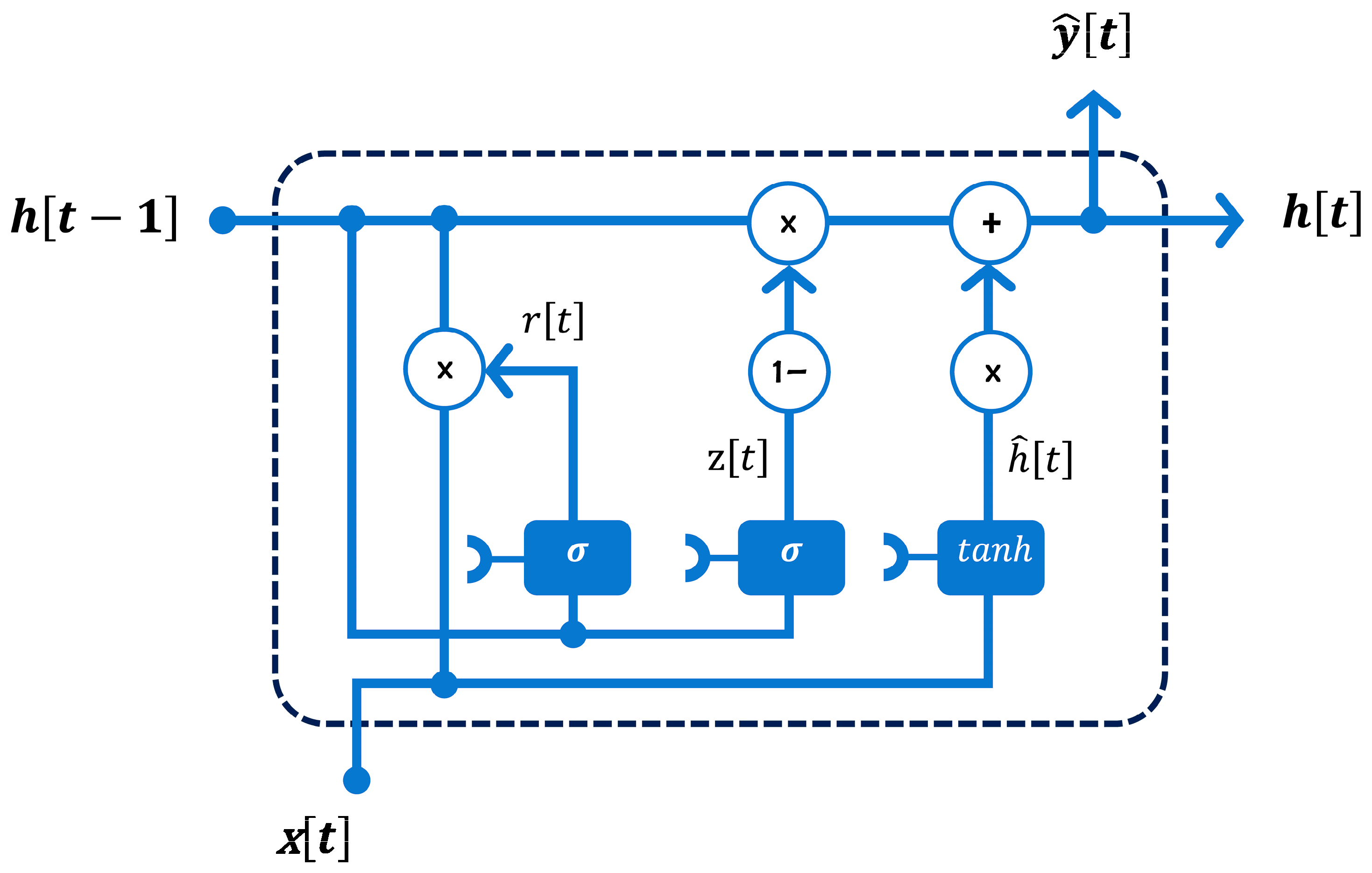
  • t a n h . : hyperbolic tangent activation function, which maps its input to the range 1 ,   1
It should be noted that sigmoid activation function, σ , is used in the update and reset gates to regulate the information flow within the network by determining how much of the previous state should be retained or updated.
The GRU’s main advantages are its lower computational cost, faster convergence, and ability to learn long-term dependencies even with limited data, while its limitations include reduced flexibility for modeling highly complex temporal relationships compared to LSTM networks.
Figure 1. GRU architecture.
Vibration 08 00070 g001
Recent studies have shown that Bidirectional Gated Recurrent Unit (BGRU) networks, which process input sequences in both forward and backward directions, can outperform traditional RNN and GRU models [32,33]. In the BGRU architecture, two parallel GRU layers are employed: one processes the input sequence in the forward direction (from the beginning to the end of the time series), while the other processes it in the backward direction (from the end to the beginning). The outputs of the two layers are then concatenated at each time step to form the final hidden representation, allowing the model to simultaneously incorporate information from both past and future observations [33,34].
This bidirectional processing enables the model to consider both past and future contextual information simultaneously, enhancing its ability to capture long-range temporal dependencies and nonlinear vibration patterns that are often present in construction-induced ground vibrations. Such an architecture allows the network to learn more comprehensive temporal features compared to unidirectional models, leading to improved generalization and predictive accuracy. Each GRU cell within the BGRU follows the same gating mechanism described in Equation (2), where the update and reset gates regulate information flow and memory retention. All network parameters are jointly optimized during training using the Adam optimizer with a mean squared error (MSE) loss function. The schematic architecture of the BGRU model is illustrated in Figure 2.

2.4. Random Forest Method

Random Forest (RF) is a powerful ML algorithm that operates by constructing multiple decision trees during training and outputs the mode of the classes (classification) or mean prediction (regression) of individual trees. Each decision tree is built using a random subset of the training data and a random subset of features at each split point, which helps reduce overfitting and improve generalization [35].
In time series forecasting, RF can be adapted by incorporating lagged values of the target variable and possibly other relevant features as input variables. This approach enables the algorithm to capture temporal dependencies and patterns in the data. The detailed explanation of RF is beyond the scope of this paper, and an interested reader is referred to [36,37] for further explanations.

2.5. ARIMA Method

ARIMA, which stands for Autoregressive Integrated Moving Average, is a statistical method widely used for time series forecasting. It combines three components: autoregression (AR), differencing (I), and moving average (MA). These components allow ARIMA to capture various patterns in time series data and are explained briefly as follows [37,38,39,40]:
Autoregression (AR): This component refers to modeling the relationship between an observation and a number of lagged observations (i.e., past values of the same time series). It captures the idea that the current value of a series can be dependent on its past values. The parameter “p” in ARIMA (p, d, q) represents the number of lagged observations included in the model.
Differencing (I): This component involves differencing the time series data to make it stationary. Stationarity is a key assumption in many time series models, including ARIMA. Differencing helps remove trends and seasonality from the data, making it easier to model. The parameter “d” in ARIMA (p, d, q) represents the degree of differencing applied to the series.
Moving Average (MA): This component models the relationship between an observation and a residual error from a moving average model applied to lagged observations. It captures short-term, random fluctuations in the series that are not accounted for by the autoregressive component. The parameter “q” in ARIMA (p, d, q) represents the number of lagged forecast errors in the prediction equation.
Combining these three components allows ARIMA to capture a wide range of time series patterns and produce accurate forecasts. However, determining the appropriate values of “p,” “d,” and “q” can be challenging and often requires statistical techniques such as model selection criteria or grid search.

2.6. Metrics for Model Evaluation

In this study, two metrics are used to evaluate different methods and compare their results: coefficient of determination (R-squared or R 2 ) and root mean squared error (RMSE). These metrics are defined in the following equations:
R 2 = 1 y i y ^ i 2 y i y ¯ 2
R M S E = i = 0 n 1 y i y ^ i 2 n
where, y i , y ^ i , and y ¯ denote the true value, predicted value, and average of the true values, respectively. Also, n is the number of observations.

3. Vibration Data Acquisition

Terrapex Environmental Ltd. (Toronto, ON M3B 2R7, Canada) [41] has provided the dataset for 12 vibration monitoring projects in Toronto, Canada. The projects’ characteristics are listed in Table 1 and Table 2. Their addresses are not provided due to privacy concerns. All vibration data are recorded using Syscom Rock devices, as shown in Figure 3.
The Bartec Syscom Rock, Sainte-Croix, Switzerland [42] is a compact vibration monitoring device for field monitoring. The unit is a wireless device with an embedded 4G LTE modem and ultra-low power components that can continuously monitor the vibrations (24 h a day) for up to six months with its internal battery. The unit is continuously connected to Syscom Cloud Software (SCS), which is software for dynamic measurement monitoring, data processing, remote parametrization, alarming, and reporting [42]. The Syscom Rock unit and SCS software comply with worldwide regulations, which allow the alarm levels to be tuned to send notifications if the vibration level exceeds a defined threshold value.
It should be noted that the vibration monitoring instruments used in this study operated at a sampling rate of 500 Hz, allowing accurate capture of the full frequency range of construction-induced vibrations (typically 5–200 Hz). However, for regulatory compliance and data management efficiency, the cloud-based monitoring system stored only the maximum PPV value within each 60-s interval. In the event of a significant vibration exceedance, the system automatically recorded a one-minute high-resolution segment before and after the event, ensuring that all vibration scenarios were captured in detail.
The dataset analyzed in this study therefore consists of the time series of maximum PPVs, which represents the information required for regulatory verification and client reporting. Accordingly, the objective of the present work is to predict the sequence of maximum PPVs over time rather than the raw high-frequency vibration waveform, as these peak values are the quantities directly used for assessing compliance with vibration threshold limits.
According to Section 363-5.2 of the Toronto Municipal Code [43], the construction vibrations should not exceed the prohibited values in Table 3, with f and P P V representing the vibration dominant frequency and peak particle velocity, respectively.
It is common practice in the industry to set a review limit that is less than the above thresholds, in order to provide sufficient reaction time for informing the construction site authorities to prevent potential exceeding vibrations. The Syscom Bartec unit records the PPV in three spatial directions: x, y, and z every 60 s. Therefore, 1440 PPV data (for each axis) would be recorded each day.

4. Problem Definition

The construction vibration data is a time series with the time axis indicating the PPV of the vibration at every minute. The direction of particle motion is important in ground vibration assessment. Generally, the particle movement has three components: vertical, horizontal longitudinal, and horizontal transverse. Since the movements are vector quantities, there would be a resultant vector that is the vectorial summation of the movements in three directions [27]. There have been debates about particle movement selection for vibration analysis. The PPV can be considered for vibration assessment in three different ways [27]:
  • Maximum of vertical, horizontal longitudinal, and horizontal transverse components.
  • Maximum value of the vector summation of the three particle velocity components at each time step.
  • Vector summation of the maximum particle velocity components regardless of the time span in which the velocities are measured [44].
This paper is grounded on the second criterion, a crucial aspect of our research. It involves measuring the peak particle velocity components in three directions at each 60-s period, with the maximum value considered as the PPV. This approach, while conservative as it considers all directions without summation, is effective in preventing vibration exceedances with a more significant safety factor.
In urban construction projects, vibration monitoring is primarily performed to ensure compliance with regulatory threshold limits, such as those established by the Toronto Municipal Code. However, compliance verification requires continuous and complete vibration records throughout the construction period. In practice, the monitoring units may become damaged due to construction activities, harsh weather conditions, or delayed maintenance, and they may also run out of battery if not replaced promptly. These issues can lead to data loss, creating gaps in the vibration record and uncertainty about whether vibration levels exceeded the allowable limits during unmonitored periods. This is a common and challenging problem in field monitoring practice. Therefore, it is crucial to develop a predictive framework capable of reconstructing missing vibration data based on previously recorded measurements. The present paper addresses this issue and evaluates three different prediction methods—BGRU, RF, and ARIMA—to estimate the ground vibration time histories for the datasets presented in Table 1.
The studied projects were selected carefully to provide a variety of potential practical cases that might happen in real projects. Some brief notes are provided about the nature of the data for each project in Table 1. The projects’ durations range from 16 to 330 days. All of the projects are vibration monitoring projects in which construction activities are performed, except project 10, which is a vibration assessment project. This project only measures the ambient vibrations in a house near a subway in Toronto to assess the potential harmful vibrations caused by the underground train movement. It should be noted that the term “event” in Table 1 refers to any vibration amplitude that exceeds the threshold limit of 5 mm/s. At this PPV value, the Bartec Syscom units will send an alert to prevent construction activities that might cause potential damage.
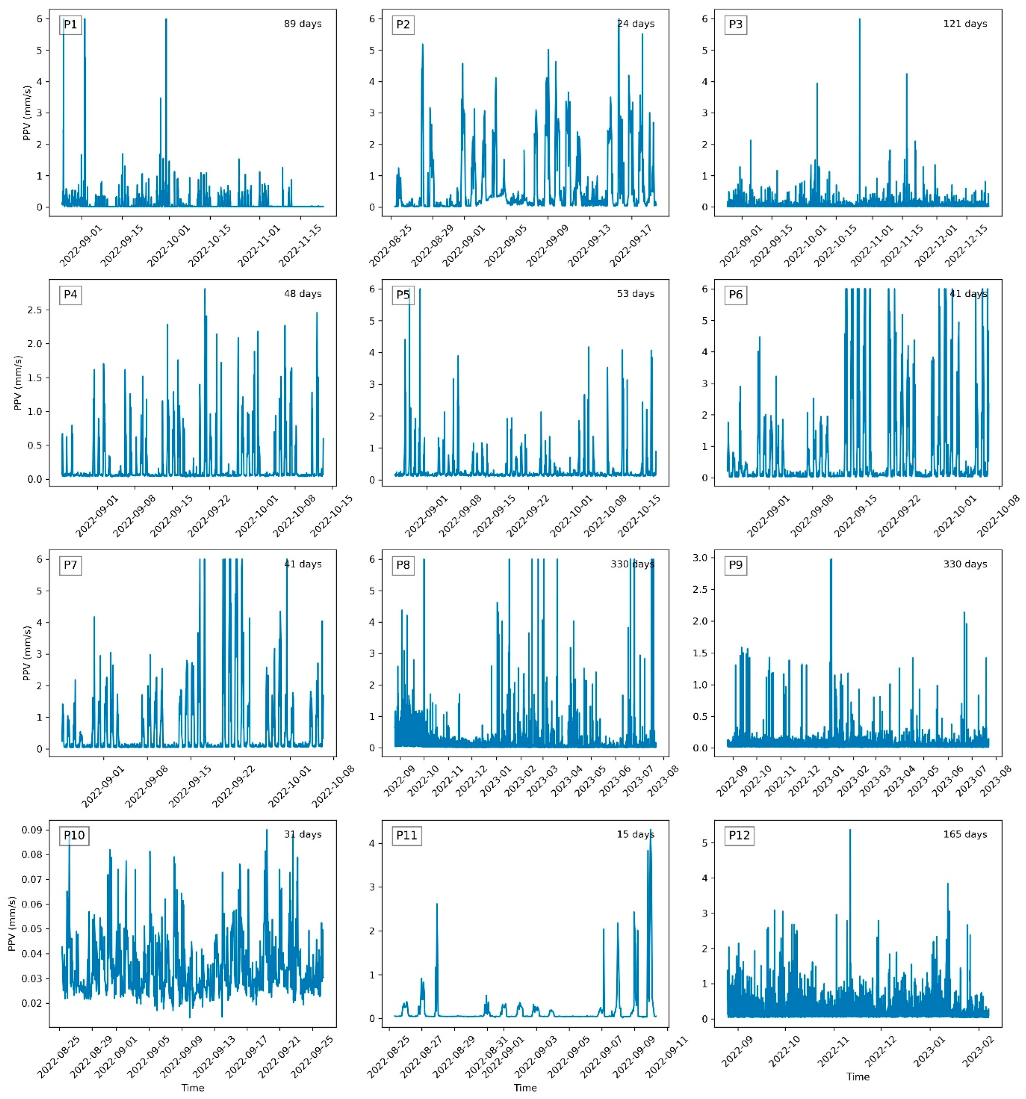
Figure 4 presents the time histories of vibration data for all twelve monitored construction projects (P1–P12). For the sake of simplicity and consistent comparison, it is assumed that the vibration units in all projects started recording the data at 8:00 AM on 25 August 2022. The time axis is shown in datetime format, and the project number, along with the monitoring duration, is indicated in each subplot. The vibration records exhibit substantial variability in both duration and amplitude across the projects.
The recording periods range from short-term campaigns such as P11 (15 days) and P2 (24 days) to long-term monitoring such as P8 and P9 (approximately 330 days). Projects P3, P6, and P12 also represent relatively extended durations (121, 141, and 165 days, respectively) with frequent high-amplitude bursts, indicating periods of intensive construction activity. In contrast, P1, P4, and P10 display shorter sequences with fewer but distinct peaks, reflecting intermittent vibration events. The maximum PPV values vary considerably—from below 1 mm/s in P10 to peaks exceeding 5 mm/s in P2, P5, and P8—demonstrating the influence of different construction methods, equipment types, and ground conditions. Overall, long-term projects (e.g., P6, P8, P9, P12) tend to exhibit distributed vibration energy with recurring peaks over time, while short-term projects (e.g., P2, P11) are characterized by dense, high-magnitude bursts concentrated within brief intervals. These differences emphasize the diverse vibration signatures produced by varying site conditions and operational durations across the studied projects, as explained in Table 2.

5. Results and Discussion

This section first elaborates on the RF, ARIMA, and BGRU models and their hyperparameters. Then, it provides time series predictions and discusses the different models’ performance.

5.1. Random Forest Hyperparameters

The performance of the random forest model highly depends on the hyperparameter tuning. The solution space for the random forest hyperparameter selection is very large, and an optimization algorithm should be used for this purpose. The grid search method is used to tune the hyperparameters. The optimal number of the hyperparameters for each dataset is presented in Table 4. The hyperparameters and ranges are explained as follows:
  • n_estimator: This parameter indicates the number of trees in the forest. More trees generally improve the model’s performance by reducing variance, but this also increases computational cost and memory usage. This parameter ranges between 100 and 1000 in this paper. Having at least 100 trees ensures that the model is robust, and going up to 1000 allows for finding the optimal balance between performance improvement and computational efficiency.
  • max_depth: This parameter defines the maximum depth of the trees and controls how deep the tree can grow. The lower and upper bounds of max_depth are 10 and 100, respectively, with increments of 10. This range is sensible for exploring both shallow and deep trees, helping to prevent overfitting and underfitting.
  • min_samples_split: This parameter controls the minimum number of samples required to split a node and helps prevent the model from creating nodes that only capture noise. A range of 2 to 20 for the minimum number of samples is considered in this paper. This range covers a variety of potential splits, ensuring that the model does not create overly specific trees while allowing for flexibility in how nodes are split.
  • min_samples_leaf: This parameter specifies the minimum number of samples required to be present at a leaf node, ensuring that each leaf contains a sufficient number of observations. A range of 1 to 20 was selected for this hyperparameter to prevent the model from becoming overly specific to the training data. The min_samples_leaf parameter was optimized using a grid search approach, where its value was systematically varied within the defined range. For each trial, model performance was evaluated through cross-validation on the training dataset, and the value yielding the lowest validation error while minimizing overfitting was selected as the optimal setting for each project, as summarized in Table 4.

5.2. ARIMA Parameters

Similarly, the grid search method is used to find optimal ARIMA parameters: p, q, and d. The autoregressive (AR) order parameter, p, ranges between 0 to 2. The differencing order parameter, q, can be either 1 or 2. The moving average (MA) order parameter, d, ranges from 0 to 2. The optimal ARIMA values for each project are provided in Table 5.

5.3. Details of the BGRU Model

Data windowing is the most critical step of the BGRU model. In this step, a sequence of data points is defined on the time series and divided into inputs and labels, as shown in Figure 5. The BGRU model fits the input data and predicts the labels. It is repeated until the desired accuracy is obtained. Then, the data will be shifted forward with “s” time steps, and a similar procedure will be repeated.
There are generally two approaches to predicting future data: single time-step and multiple time-step. In the single time-step approach, only one data (label width = 1) is predicted based on the previous “m + 1” data. In contrast, in the multiple time-step approach, more than one data is predicted considering the previous data, i.e., “label width > 1”. This paper considers a single-data approach for the predictions with the input, label, and shift width values of 6, 1, and 1, respectively. For better clarity, the first three data windows are shown in Figure 6.
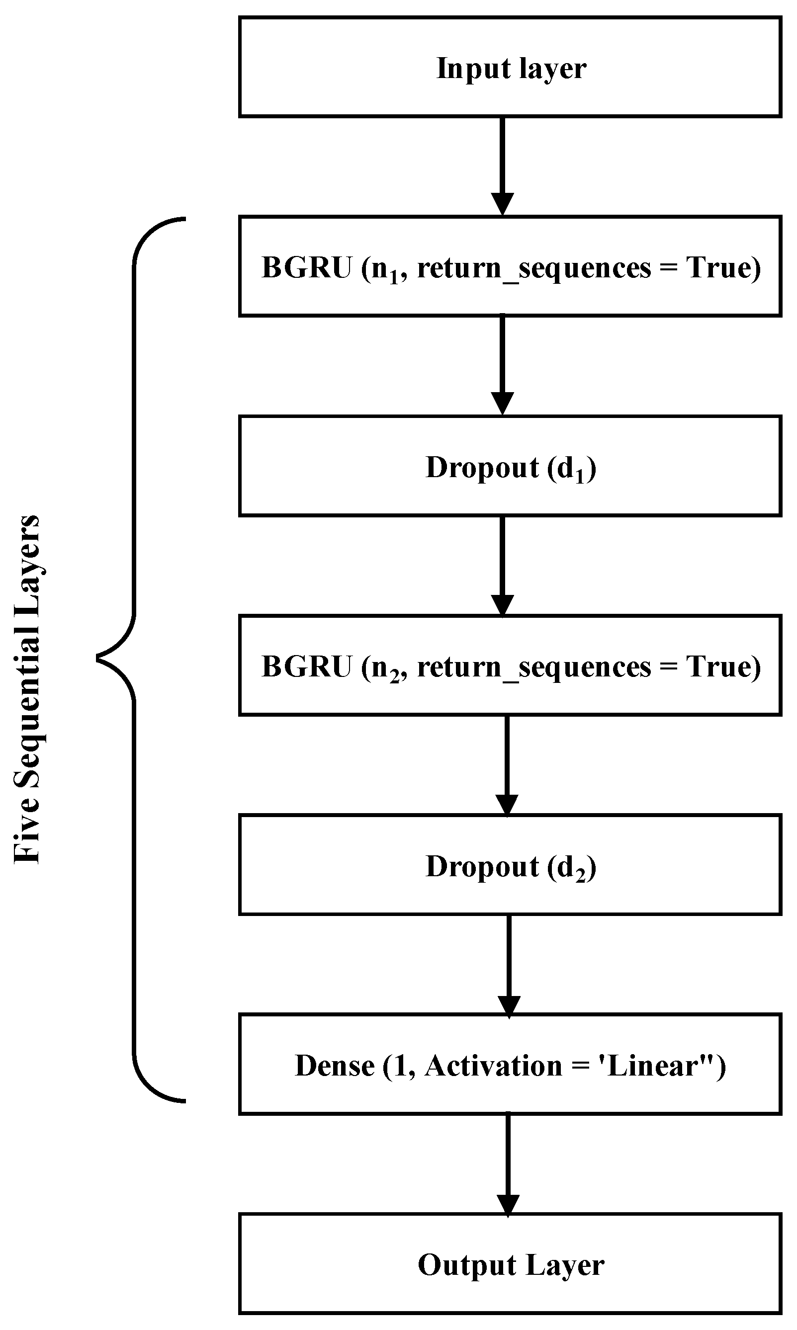
Keras [45] is a high-level API in the TensorFlow [46] software library that can be used to solve problems with deep learning methods. The Sequential model in Keras allows for the stacking of different layers in the network. The architecture of the sequential neural network model, used in this paper, is shown in Figure 7. The model contains five sequential layers: 2 “BGRU” layers with n 1 and n 2 neurons, 2 “Dropout” layers with the dropout rate of d 1 and d 2 , and one Dense (fully connected) layer with 1 unit and linear activation function. It should be noted that this architecture is selected among a lot of different possible combinations by checking the accuracy of the output data. The model’s hyperparameters include: neuron numbers, dropout rate, epoch numbers, patience for early stopping, type of optimizer, learning rate, batch size, and data window lengths. These parameters are tuned by running the model for the various datasets. These hyperparameters are listed in Table 6.

5.4. Discussions

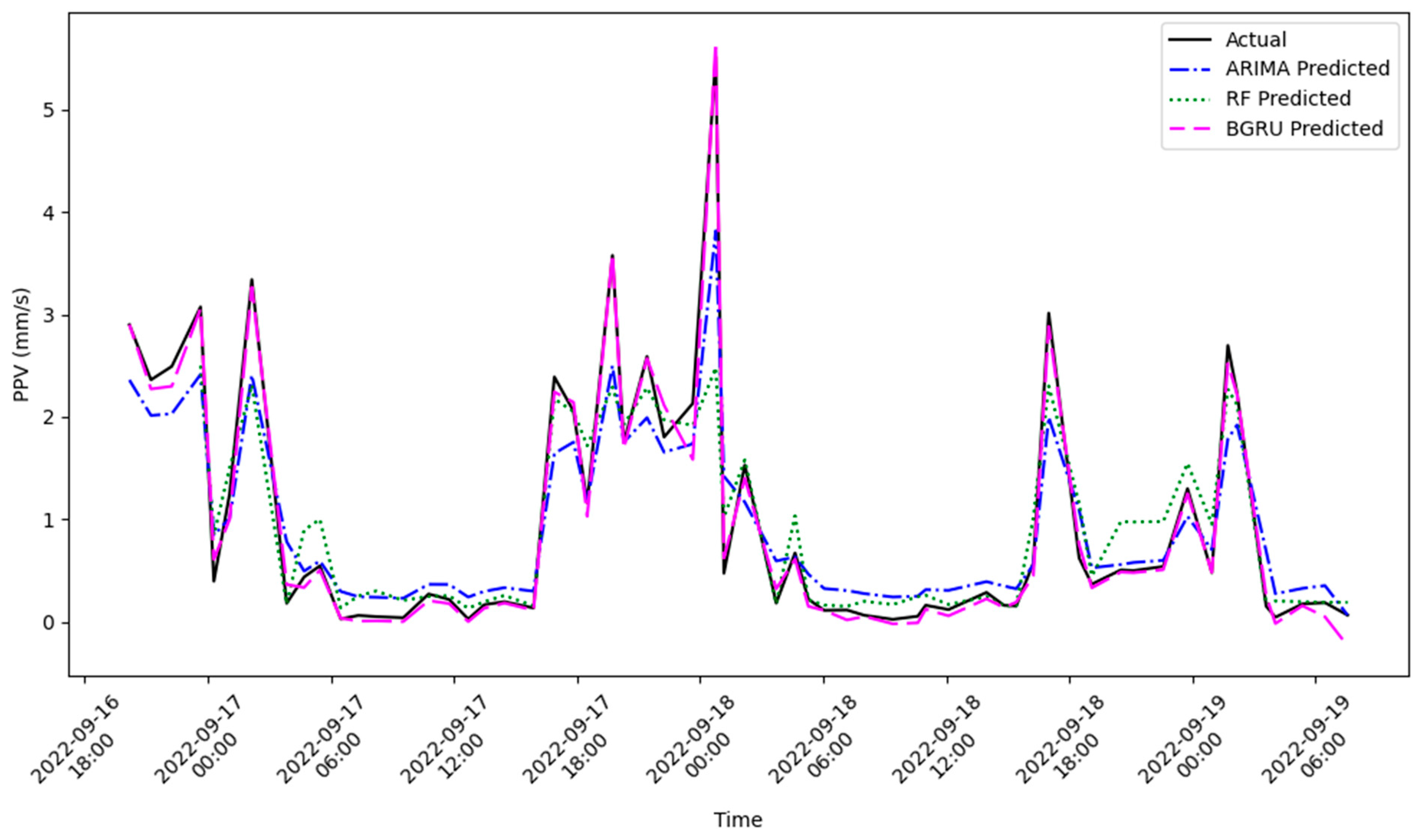
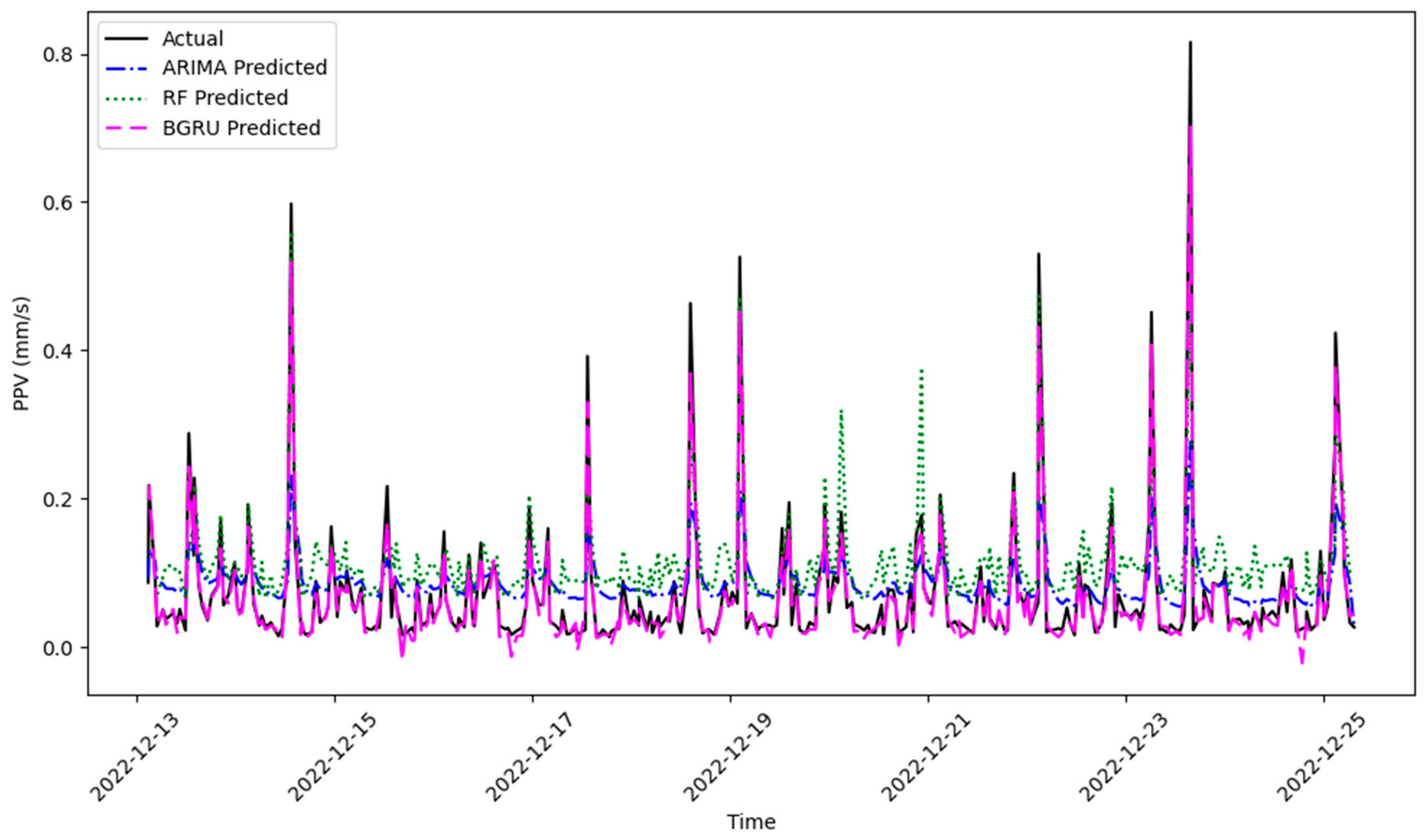
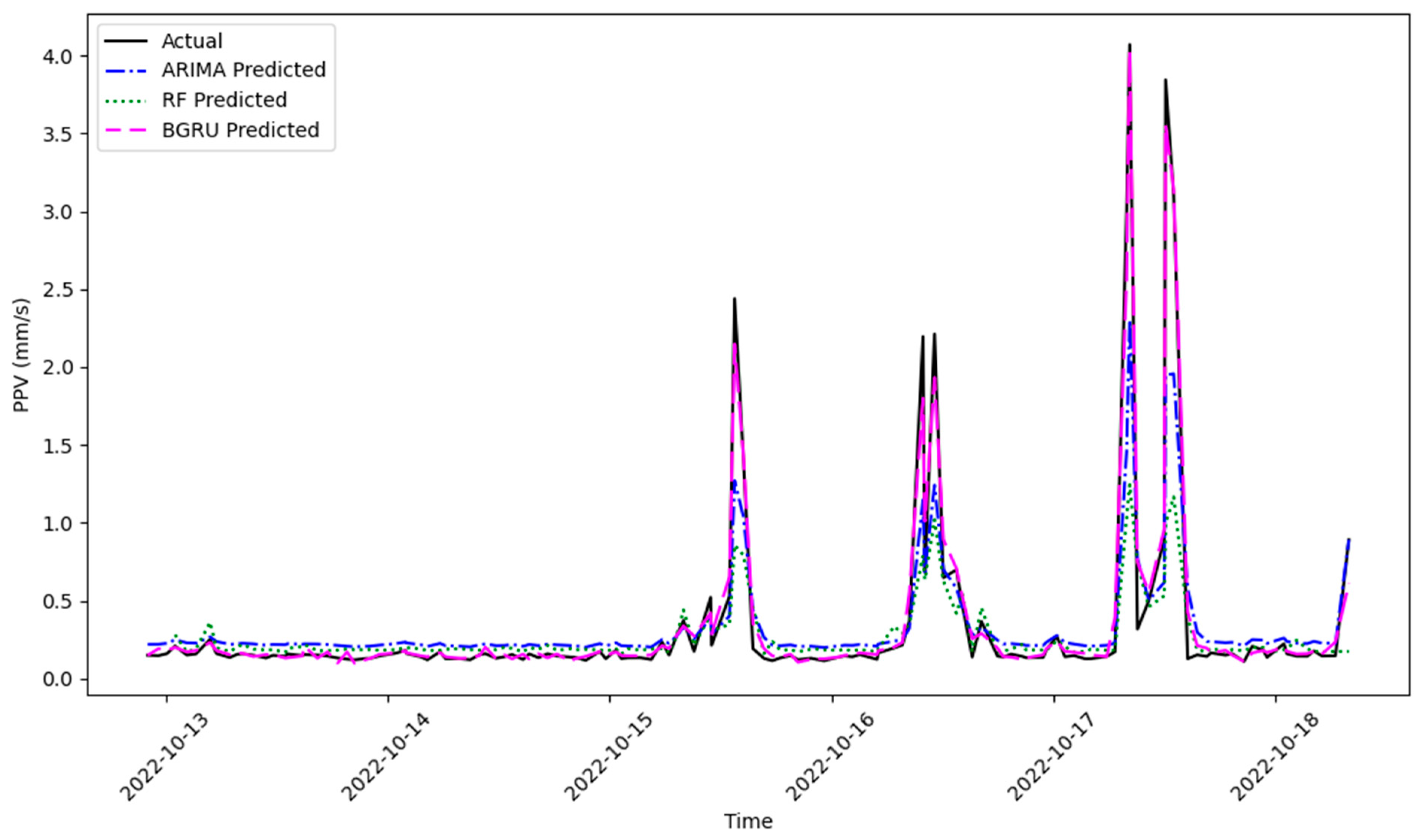
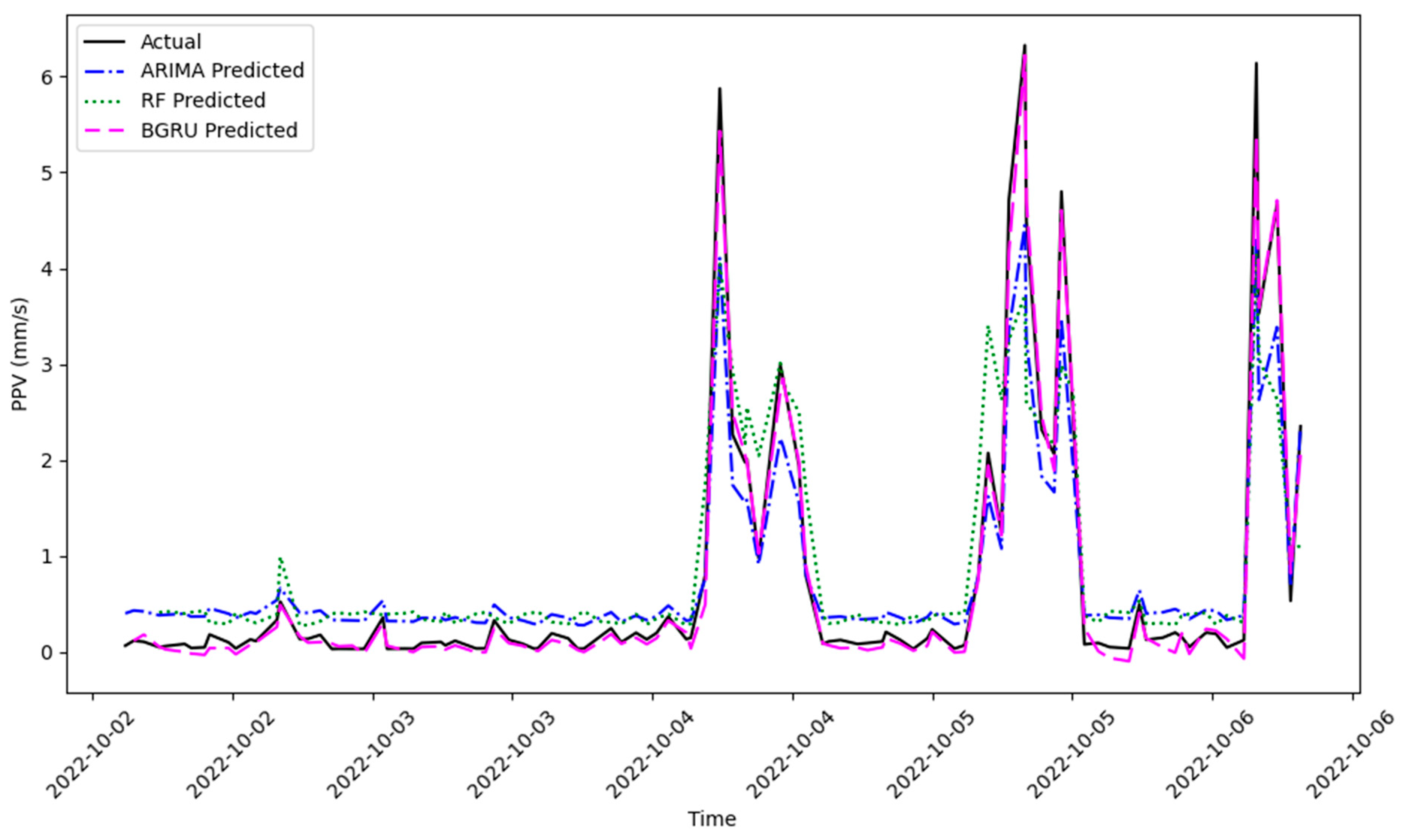
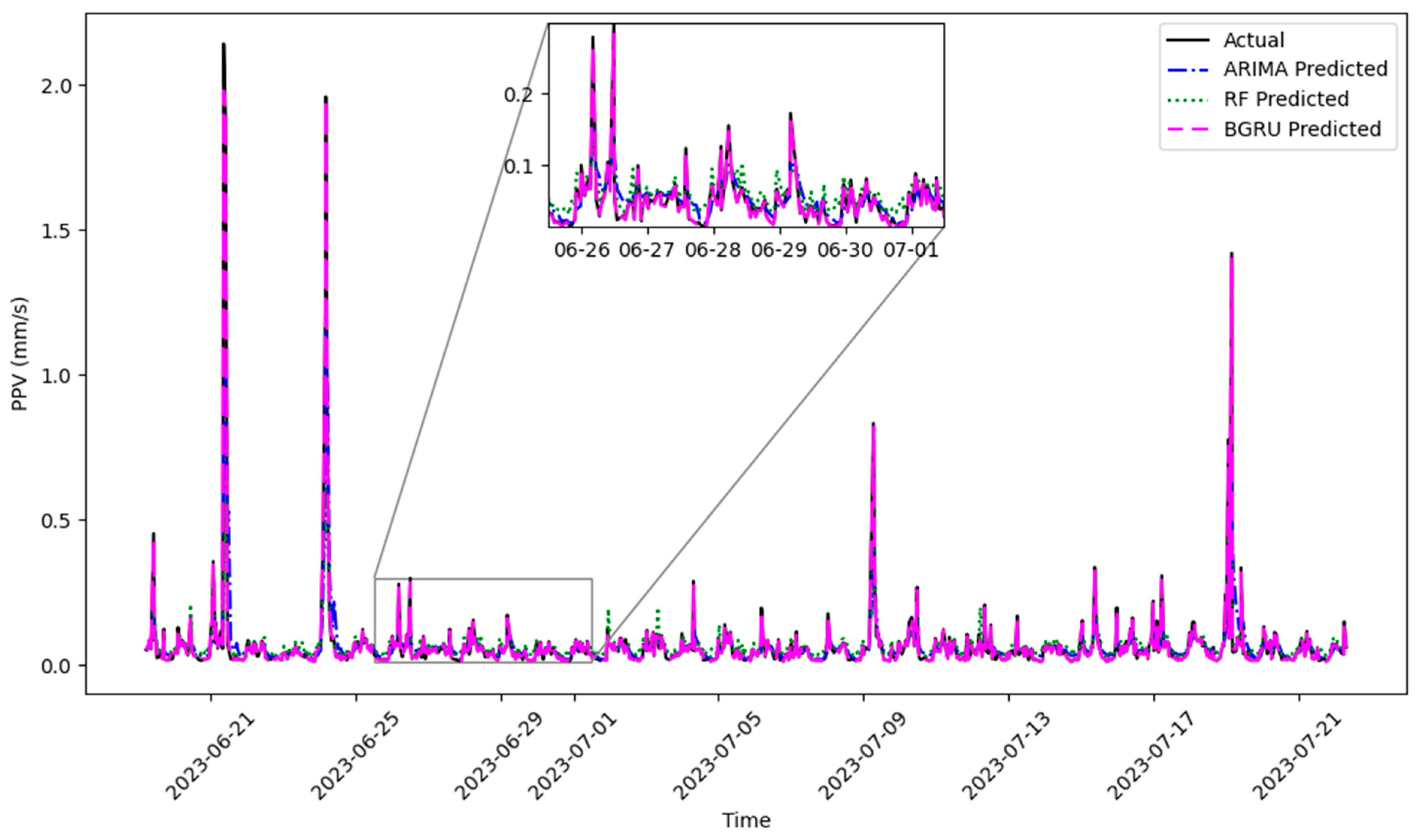
The metrics of the predictions are listed in Table 7. These metrics are for the testing data. The train, validation, and test split ratios are 0.7, 0.2, and 0.1, as indicated in Table 6. Figure 8 shows the training, validation, and test predictions with the BGRU method in Project 1 as a sample. The predicted results are shown in Figure 9, Figure 10, Figure 11, Figure 12, Figure 13, Figure 14, Figure 15, Figure 16, Figure 17, Figure 18, Figure 19 and Figure 20, for projects 1 to 12, respectively.
The prediction metrics indicate that the BGRU model forecasts the ground vibrations with very high accuracy and is much better than ARIMA and RF methods. The coefficient of determination ( R 2 ) is close to one in all of the projects except project numbers 1, 3, and 11. The R 2 for BGRU ranges from 83.5 to 99.8%, while it ranges from a negative value to 78.9% for RF, and a negative value to 88.1% for ARIMA. Generally, the RF model is inferior and cannot predict the ground vibrations correctly. The same trend exists for the RMSE metric. The RMSE value is significantly smaller in the BGRU method compared to ARIMA and RF. Also, the RMSE value for the ARIMA model is generally smaller than that for RF.
The poor performance of the ARIMA and RF predicting models for project 1 relates to the nature of the vibration data. The total ground vibration time history for project 1 is shown in Figure 4, which shows the ground vibration in the basement slab of a two-story house for 89 days. There are some notable vibration events in this data before the date of 1 October 2022. This portion of data is used for the training. On the other hand, the ground vibration amplitudes are negligible after 7 November 2022, and this portion of the data is used for testing the algorithm. From a physical point of view, the negligible data after 7 November 2022 in project 1 is recorded after the construction vibration ended. Therefore, it basically shows the ambient ground vibration existing at that location. Due to this reason, the predicting algorithms cannot forecast this portion of data because they are already trained with the construction data. The RF and ARIMA models’ performances are very poor for this project as they have negative R 2 values. The poor performance is also obvious visually in Figure 9. Although the performance of the BGRU model is relatively poor for project 1, in comparison to the other projects, it still provides a high R 2 value of 83.5% and has a better performance compared to ARIMA and RF models. This observation illustrates that the BGRU model is very powerful in predicting ground vibrations. The vibration data before 7 November 2022 includes both ambient and construction activity vibrations. The BGRU model is trained for this data; however, it captures the nature of the ambient vibrations and predicts the ambient vibrations much better than the other models. The training data completely mistake ARIMA and RF models and cannot distinguish the ambient vibration nature in mixed construction-induced and ambient ground vibration data.
It should be noted that all of the methods, including the ARIMA and RF methods, perform well in predicting vibration time histories. This happens because the nature of the training and testing data is similar, as both sets of data have a significant number of events.
The R 2 of the BGRU, RF, and ARIMA methods for the vibration data of project 3 is 95.4, 51.9, and 43.4%, respectively. This project has significant peaks and events in the training data, while there is no peak in the testing data. Therefore, the ground vibration predictions might be a little biased. This can be observed by the negative oscillations of the BGRU method, as seen in Figure 11. Furthermore, the peak amplitudes are slightly smaller in the BGRU method compared to the actual data. Although the prediction metric of R 2 is larger in the RF method than the ARIMA method, the visual inspection of the data in Figure 11 does not show a clear superiority in the prediction. In fact, both RF and ARIMA methods provide averaged ground vibration data without correct vibration peaks.
The vibration time history for project 10 in Figure 4 shows that the ground vibration amplitudes are very small in this project because no specific construction activity is performed at this site, and the vibrations are due to normal ambient activities. The R 2   prediction metric for BGRU, RF, and ARIMA methods for this project is 99.3, 32.2, and 57.9%, respectively, which shows a very high accuracy of the BGRU method to capture the ambient vibrations. The visual assessment of the predictions in Figure 18 shows the BGRU method captures the time and amplitudes of the ambient vibration peaks accurately. In contrast, the RF method averages the amplitudes without any comparable peak value. The ARIMA method predictions have some peaks, but they have time shifts and cannot be easily related to any specific peak in the actual data.
The prediction of the vibrations in project 11 is similar to project 1. The total time history of the vibrations for project 11 in Figure 4 shows that the training data do not include peaks and events; however, some obvious peaks are observed in the testing data. The performance of RF method is very poor for this project, and its R 2 is 8.1%, per Table 7. The ARIMA method performs quite well for this project and has a R 2 of 68.9%, per Table 7. The BGRU method predicts the vibrations much better than the RF and ARIMA methods, and its R 2 is 94.5%. The visual assessment of the predictions in Figure 19 indicates that the BGRU method predicts the amplitude and time of the peak vibration very well at 19:00 on the date 9 September 2022. It also predicts the amplitude of the peak vibration at time 23:00 on the same date with a lag of about an hour.
In the other projects (e.g., P2, P4, P5, P6, P7, P8, and P9), the BGRU method outperformed the RF and ARIMA methods. The BGRU method fully captures the nature of the vibrations and predicts them accurately. Furthermore, the ARIMA method performs better than the RF method in all projects except project 3. Neither RF nor ARIMA projects can capture the time and amplitude of the vibrations accurately. They somehow provide an averaged estimation of the ground vibrations, which is not appropriate for the nature of construction-induced vibrations because the peaks that pass the threshold limit are only important.
The observed differences in performance among the models can be explained as follows:
The ARIMA model, being inherently linear, struggles to capture regime shifts and sharp, sparse peaks, as its differencing process tends to smooth out spikes and distort timing information. The RF model, which relies on fixed lags and operates in a non-autoregressive manner during inference (i.e., without closed-loop recursion), tends to average predictions and underrepresent peak amplitudes; moreover, its decision tree structure does not inherently capture temporal dependencies or gating mechanisms. In contrast, the BGRU model employs gated additive updates that preserve major temporal states while suppressing noise. The bidirectional training further enhances gradient propagation and credit assignment, leading to more accurate peak timing and smoother transition dynamics.
The variations in error levels across the twelve projects are primarily attributed to the different characteristics of the recorded vibration signals, including the duration of monitoring, frequency and magnitude of vibration events, and the relative dominance of construction versus ambient sources. Projects involving longer monitoring durations and multiple active construction phases (e.g., P6, P8, P9, and P12) generally yield smaller prediction errors because the models are exposed to a more diverse and representative set of vibration patterns during training. In contrast, short-duration projects or those with unevenly distributed events (e.g., P1, P3, and P11) exhibit higher error levels, as their testing segments often contain limited or atypical vibration patterns that differ significantly from the training data. This mismatch reduces the ability of the learning models—particularly ARIMA and RF—to generalize across time segments.
Furthermore, the signal-to-noise ratio and temporal sparsity of vibration peaks play an important role in model performance. Projects characterized by low-amplitude ambient vibrations or sparse impulsive events (such as P1 and P10) tend to produce higher RMSE values and lower R 2 scores for ARIMA and RF models because these models average out low-energy signals and fail to reconstruct infrequent peaks. The BGRU model, however, benefits from its gated recurrent structure and bidirectional memory, which allow it to adapt to sudden amplitude changes and maintain contextual awareness across time. Consequently, its error levels remain consistently low even in projects with intermittent or nonstationary vibration patterns. These findings highlight that the observed differences in prediction metrics reflect the underlying variability of real construction vibration environments rather than inconsistencies in the modeling framework itself.

5.5. Notes on the Optimization of Data and Methods

In practical construction environments, vibration signals are often influenced by nonlinear disturbances, uncertainties in soil and material properties, and signal propagation delays. Traditional sequential models, such as BGRU, while effective in capturing temporal dependencies, do not explicitly account for these nonlinear and time-delay effects. Recent studies have proposed advanced neural frameworks to address such challenges. For example, Chen et al. [47] developed a neural network–based reinforcement iterative learning fault estimation scheme that enhances robustness and adaptability in nonlinear uncertain systems with time delays through iterative optimization and reinforcement-based adaptive mechanisms. Their approach demonstrates how dynamic learning processes can improve estimation accuracy and stability under uncertain and delayed conditions.
Moreover, in field applications such as real-time construction vibration monitoring, models must be computationally efficient to enable deployment on edge devices—compact units installed near the vibration source for on-site data processing. Lightweight architectures have therefore become increasingly important. Hou et al. [48] introduced the Global–Local Parallel Transformer (GLP-Transformer), which combines the parameter efficiency of convolutional operations with the global feature extraction capability of transformer networks. This model significantly reduces computational complexity while maintaining strong generalization performance, making it suitable for deployment in resource-constrained environments.
In future developments, integrating such adaptive learning mechanisms and lightweight architectural principles into the BGRU framework could further enhance its robustness, efficiency, and feasibility for real-time, on-site vibration prediction and monitoring.

5.6. Frequency-Domain Considerations, Data Limitations, Feature Sensitivity

The dynamic response of soil–structure systems is inherently frequency-dependent, and resonance phenomena can amplify vibration effects even when the time-domain peak particle velocity (PPV) values appear moderate. While recognizing the importance of these mechanisms, the present study focuses on the time-domain prediction of vibration records, as the available datasets were obtained from real construction monitoring projects carried out primarily for regulatory compliance. These monitoring programs were designed to ensure that vibration levels remained below the allowable limits defined in the Toronto Municipal Code, which evaluates compliance based on PPV thresholds rather than frequency-domain parameters.
Due to this practical context, detailed geotechnical and structural data—such as soil layering, stiffness profiles, and building dynamic properties—were not available, making a full frequency-response or spectral analysis infeasible. Nevertheless, incorporating frequency-domain features could provide deeper physical interpretability and help identify potential resonance or amplification effects that influence soil and structural responses.
The BGRU architecture inherently captures temporal dependencies by processing the input sequence in both forward and backward directions. However, it does not explicitly quantify temporal sensitivity, i.e., the relative importance of each past input in influencing the predicted PPV. To enhance interpretability, future developments could include temporal-sensitivity analyses to examine how different time steps contribute to the prediction.
Future research will also aim to integrate the proposed predictive framework with Fourier- or wavelet-based frequency-response analyses once datasets containing comprehensive soil and structural information become available. Combining frequency-domain modeling with temporal-sensitivity analysis would extend the applicability of the BGRU framework beyond regulatory compliance toward engineering evaluation, vibration mitigation, and site-specific dynamic characterization, enabling a more complete understanding of ground vibration behavior across both the time and frequency domains.

5.7. Practical Deployment Considerations

All models were executed on a workstation equipped with an 11th Gen Intel(R) Core(TM) i7-1185G7 @ 3.00 GHz processor and 16 GB RAM. Among the three prediction methods, the BGRU model had the highest computational cost because of its large number of trainable parameters and complex recurrent structure. The Random Forest (RF) model also required notable resources due to the generation of multiple decision trees, while the ARIMA model was the least computationally demanding. Depending on the dataset, the computation time for the BGRU model was approximately five to ten times longer than that of the RF model, whereas the ARIMA runtime was negligible. Despite its higher computational cost, the BGRU approach achieved substantially greater prediction accuracy, which is essential for reliable vibration assessment and compliance verification.
Regarding model retraining, the vibration datasets used in this study varied in length. Each series was divided into training, validation, and testing subsets. For longer time series, the model implicitly adapted to evolving site conditions—such as changes in equipment type or construction stage—thereby achieving a form of inherent retraining. For shorter datasets, this effect was naturally more limited. In practical deployment, the model could be periodically retrained (e.g., weekly or monthly) as new data become available, following the standard definition of retraining as the process of refining an existing model to maintain or improve performance when exposed to updated datasets.
The datasets analyzed in this study contained very few missing values. Minor gaps were addressed through simple linear interpolation to maintain data continuity. In future real-time applications, the proposed BGRU framework can be directly integrated into continuous monitoring systems to reconstruct missing or corrupted data segments, ensuring uninterrupted compliance tracking and improving the robustness of vibration monitoring programs.

6. Conclusions

This paper uses a bidirectional gated recurrent unit (BGRU) neural network to predict the construction-induced ground vibrations in 12 projects in the City of Toronto, Canada. The BGRU predicted results are compared to the predictions of the Random Forest (RF) method and statistical method of ARIMA. The major findings of this paper are itemized as follows:
  • The BGRU method’s superior performance not only outperforms the RF and ARIMA methods but also underscores the significance of our findings in predicting construction-induced ground vibrations.
  • The BGRU method can distinguish between construction-induced and ambient vibration data in the training step. Therefore, it can predict either type of vibration data even if trained by a mixed type of database.
  • The RF and ARIMA methods cannot distinguish between construction-induced and ambient vibration data in the training step. Therefore, they performed poorly (i.e., negative coefficient of determination) when the model was prepared using a mixed data type but was used to predict either ambient or construction-induced data.
  • The BGRU method can well predict different types of construction-induced and ambient ground vibrations with various durations.
  • The ARIMA method performs better than the RF method because it is based on the statistical concept of serial correlation, in which past data points affect future data points.
  • The coefficient of determination for BGRU ranges from 83.5 to 99.8%, while its vmaximum value for RF and ARIMA methods is 78.9 and 88.1%, respectively.
  • The coefficient of determination for the RF and ARIMA methods is negative in some projects because the nature of the testing and training data is different.
  • In addition to the metric quantities, the predicted results’ visual inspection shows the obvious superiority of the BGRU method. This method predicts the amplitude of the peaks and the time of their occurrence very well.
It should be noted that, in practical terms, the proposed BGRU-based forecasting can be embedded directly into construction management workflows to improve compliance, risk control, and resource use. By generating short-horizon predictions of PPV time series (not just peak values), the model can flag likely exceedances before they occur, enabling contractors to adjust operations dynamically (e.g., sequencing, equipment choice, compaction settings, working hours) to keep vibrations within municipal limits. When monitoring units fail or data are intermittently lost, the forecasts can fill gaps for continuity of records, strengthening permit applications, compliance reporting, and post-event forensics. Scenario testing (“what-if” runs) can support preconstruction risk assessments and method statements, while predictive accuracy at ambient and construction levels helps optimize the number and placement of monitors across a site. The outputs can also feed digital dashboards and automated alerting systems, improving communication with stakeholders (owners, neighbors, and regulators) and focusing site resources where risk is highest. Overall, integrating the BGRU forecasts with existing monitoring platforms provides proactive decision support that complements conventional measurement, reduces unnecessary shutdowns, and documents due diligence throughout the project lifecycle.

Author Contributions

Conceptualization, R.R.-D., K.E. and M.N.; methodology, R.R.-D., K.E. and M.N.; formal analysis and validation, R.R.-D., K.E.; resources, K.E.; data curation, R.R.-D.; writing—original draft preparation, R.R.-D.; writing—review and editing, K.E., and M.N.; visualization, R.R.-D.; supervision, K.E. and M.N.; project administration, K.E.; funding acquisition, K.E. All authors contributed to the study conception and design. All authors have read and agreed to the published version of the manuscript.

Funding

The Mitacs Elevate Postdoctoral Fellowship Program, under reference number IT36984, and Terrapex Environmental Ltd.

Data Availability Statement

The data used in this research will be made available upon reasonable request.

Acknowledgments

The authors would like to thank the Mitacs Elevate Postdoctoral Fellowship Program and Terrapex Environmental Ltd. for their support.

Conflicts of Interest

Meysam Najari is an employee of Terrapex Environmental Ltd. The paper reflects the views of the scientists and not the company. The authors have no competing interests to declare that are relevant to the content of this article.

References

  1. Colaço, A.; Costa, P.A.; Parente, C.; Abouelmaty, A.M. Vibrations Induced by a Low Dynamic Loading on a Driven Pile: Numerical Prediction and Experimental Validation. Vibration 2022, 5, 829–845. [Google Scholar] [CrossRef]
  2. Abouelmaty, A.M.; Colaço, A.; Alves Costa, P. User-Friendly Tool for Expedited Ground Vibration Assessment Induced by Impact Pile Driving. Vibration 2025, 8, 17. [Google Scholar] [CrossRef]
  3. Wang, S.; Zhu, S. Impact source localization and vibration intensity prediction on construction sites. Measurement 2021, 175, 109148. [Google Scholar] [CrossRef]
  4. Hasanipanah, M.; Monjezi, M.; Shahnazar, A.; Armaghani, D.J.; Farazmand, A. Feasibility of indirect determination of blast induced ground vibration based on support vector machine. Measurement 2015, 75, 289–297. [Google Scholar] [CrossRef]
  5. He, Y.; Peng, L.; He, K.; Guan, Q.; Han, J.; Xiao, X.; Sheng, X. Analysis of uncertainty and variation in underground train-induced vibration based on measured data. Measurement 2023, 222, 113600. [Google Scholar] [CrossRef]
  6. Wang, I.-T. Field experiments and numerical analysis of the ground vibration isolation of shock wave propagation under explosion shock loading. Vibration 2019, 2, 300–310. [Google Scholar] [CrossRef]
  7. Rajabi, A.M.; Vafaee, A. Prediction of blast-induced ground vibration using empirical models and artificial neural network (Bakhtiari Dam access tunnel, as a case study). J. Vib. Control 2020, 26, 520–531. [Google Scholar] [CrossRef]
  8. Kumar, R.; Choudhury, D.; Bhargava, K. Determination of blast-induced ground vibration equations for rocks using mechanical and geological properties. J. Rock Mech. Geotech. Eng. 2016, 8, 341–349. [Google Scholar] [CrossRef]
  9. Triepaischajonsak, N.; Thompson, D. A hybrid modelling approach for predicting ground vibration from trains. J. Sound Vib. 2015, 335, 147–173. [Google Scholar] [CrossRef]
  10. Faizan, A.A.; Kırtel, O.; Çelebi, E.; Zülfikar, A.C.; Göktepe, F. Experimental validation of a simplified numerical model to predict train-induced ground vibrations. Comput. Geotech. 2022, 141, 104547. [Google Scholar] [CrossRef]
  11. Esmaeili, M.H.; Haft-Cheshmeh, Y.M. Dynamic characteristics of elastomeric materials used as railway vibration mitigation measures considering the effect of shape factor. Measurement 2024, 236, 115058. [Google Scholar] [CrossRef]
  12. Zhang, H.; Zhang, S.; Li, Y.; Liu, G.; Zheng, Y.; Jiang, Z. Prediction and Control Method of Long-Term Vehicle-Induced Settlement of High-Speed Railway Tunnel in Diatomite Stratum. J. Vib. Eng. Technol. 2023, 11, 2297–2307. [Google Scholar] [CrossRef]
  13. Toygar, O.; Ulgen, D.; Fidan, N.B. Experimental Study on Reutilization of Waste Rubber Chips with Sheetpiles as a Coupled-Wave Barrier to Reduce Ground-Borne Vibrations. J. Vib. Eng. Technol. 2024, 12, 8451–8463. [Google Scholar] [CrossRef]
  14. Kedia, N.K.; Kumar, A.; Singh, Y. Prediction of underground metro train-induced ground vibration using hybrid PSO-ANN approach. Neural Comput. Appl. 2023, 35, 8171–8195. [Google Scholar] [CrossRef]
  15. Amiri, M.; Hasanipanah, M.; Bakhshandeh Amnieh, H. Predicting ground vibration induced by rock blasting using a novel hybrid of neural network and itemset mining. Neural Comput. Appl. 2020, 32, 14681–14699. [Google Scholar] [CrossRef]
  16. Ulgen, D.; Ertugrul, O.; Ozkan, M. Measurement of ground borne vibrations for foundation design and vibration isolation of a high-precision instrument. Measurement 2016, 93, 385–396. [Google Scholar] [CrossRef]
  17. Lurcock, D.; Thompson, D. A new empirical prediction approach for ground borne vibration in buildings. In Proceedings of the International Congress on Sound and Vibration, London, UK, 23–27 July 2017. [Google Scholar]
  18. Moghadam, A.E.; Rafiee-Dehkharghani, R. Optimal design of wave barriers in dry and saturated poroelastic grounds using covariance matrix adaptation evolution strategy. Comput. Geotech. 2021, 133, 104015. [Google Scholar] [CrossRef]
  19. Zhou, J.; Asteris, P.G.; Armaghani, D.J.; Pham, B.T. Prediction of ground vibration induced by blasting operations through the use of the Bayesian Network and random forest models. Soil Dyn. Earthq. Eng. 2020, 139, 106390. [Google Scholar] [CrossRef]
  20. Lu, Y. Underground blast induced ground shock and its modelling using artificial neural network. Comput. Geotech. 2005, 32, 164–178. [Google Scholar] [CrossRef]
  21. Khandelwal, M. Evaluation and prediction of blast-induced ground vibration using support vector machine. Int. J. Rock Mech. Min. Sci. 2010, 47, 509–516. [Google Scholar] [CrossRef]
  22. Qiu, Y.; Zhou, J.; Khandelwal, M.; Yang, H.; Yang, P.; Li, C. Performance evaluation of hybrid WOA-XGBoost, GWO-XGBoost and BO-XGBoost models to predict blast-induced ground vibration. Eng. Comput. 2022, 38 (Suppl. S5), 4145–4162. [Google Scholar] [CrossRef]
  23. Bui, X.-N.; Nguyen, H.; Tran, Q.-H.; Nguyen, D.-A.; Bui, H.-B. Predicting blast-induced ground vibration in quarries using adaptive fuzzy inference neural network and Moth–Flame optimization. Nat. Resour. Res. 2021, 30, 4719–4734. [Google Scholar] [CrossRef]
  24. Yun, S.; Kang, J.-M.; Ha, J.; Lee, S.; Ryu, D.-W.; Kwon, J.; Kim, I.-M. Deep learning-based ground vibration monitoring: Reinforcement learning and RNN–CNN approach. IEEE Geosci. Remote Sens. Lett. 2021, 19, 7502905. [Google Scholar] [CrossRef]
  25. Sherstinsky, A. Fundamentals of recurrent neural network (RNN) and long short-term memory (LSTM) network. Phys. D Nonlinear Phenom. 2020, 404, 132306. [Google Scholar] [CrossRef]
  26. Lipton, Z.C.; Berkowitz, J.; Elkan, C. A critical review of recurrent neural networks for sequence learning. arXiv 2015, arXiv:1506.00019. [Google Scholar] [CrossRef]
  27. CDOT. Transportation and Construction Vibration Guidance Manual; CDOT: New Delhi, India, 2013. [Google Scholar]
  28. Richart, F.E.; Hall, J.R.; Woods, R.D. Vibrations of Soils and Foundations; Prentice-Hall: Hoboken, NJ, USA, 1970. [Google Scholar]
  29. Amanat, S.; Gholami, K.; Rafiee-Dehkharghani, R.; Bansal, D. Modified non-dominated sorting genetic algorithm-II for the optimal design of soil-concrete periodic plane wave barriers. Comput. Geotech. 2024, 165, 105947. [Google Scholar] [CrossRef]
  30. Dey, R.; Salem, F.M. Gate-variants of gated recurrent unit (GRU) neural networks. In Proceedings of the 2017 IEEE 60th International Midwest Symposium on Circuits and Systems (MWSCAS), Boston, MA, USA, 6–9 August 2017; IEEE: Piscataway, NJ, USA, 2017. [Google Scholar]
  31. Zhang, X.; Kuehnelt, H.; De Roeck, W. Traffic noise prediction applying multivariate bi-directional recurrent neural network. Appl. Sci. 2021, 11, 2714. [Google Scholar] [CrossRef]
  32. Schuster, M.; Paliwal, K.K. Bidirectional recurrent neural networks. IEEE Trans. Signal Process. 1997, 45, 2673–2681. [Google Scholar] [CrossRef]
  33. Chung, J.; Gulcehre, C.; Cho, K.; Bengio, Y. Gated feedback recurrent neural networks. In Proceedings of the International Conference on Machine Learning, Lille, France, 7–9 July 2015. [Google Scholar]
  34. Chughtai, J.-u.-R.; Haq, I.u.; Islam, S.u.; Gani, A. A heterogeneous ensemble approach for travel time prediction using hybridized feature spaces and support vector regression. Sensors 2022, 22, 9735. [Google Scholar] [CrossRef]
  35. Breiman, L. Random forests. Mach. Learn. 2001, 45, 5–32. [Google Scholar] [CrossRef]
  36. Talagala, T.S.; Hyndman, R.J.; Athanasopoulos, G. Meta-learning how to forecast time series. Monash Econom. Bus. Stat. Work. Pap. 2018, 6, 16. [Google Scholar] [CrossRef]
  37. Hyndman, R.J.; Athanasopoulos, G. Forecasting: Principles and Practice; OTexts: Melbourne, Australia, 2018. [Google Scholar]
  38. Box, G.E.; Jenkins, G.M.; Reinsel, G.C.; Ljung, G.M. Time Series Analysis: Forecasting and Control; John Wiley & Sons: Hoboken, NJ, USA, 2015. [Google Scholar]
  39. Brockwell, P.J.; Davis, R.A. Introduction to Time Series and Forecasting; Springer: Berlin/Heidelberg, Germany, 2002. [Google Scholar]
  40. Wei, W.W. Univariate and Multivariate Methods. Time Series Analysis; Greg Tobin: West Orange, NJ, USA, 2006. [Google Scholar]
  41. Terrapex Environmental Ltd. 2024. Available online: https://terrapex.com/ (accessed on 20 October 2024).
  42. Syscom. BARTEC SYSCOM. 2024. Available online: https://www.syscom.ch/documentation (accessed on 18 November 2024).
  43. Johnston, W. Chapter 363, Building Construction and Demolition. In Toronto Municipal Code; City of Toronto: Toronto, ON, Canada, 2023. [Google Scholar]
  44. Hiller, D.; Crabb, G. Groundborne Vibration Caused by Mechanised Construction Works; Transport Research Laboratory: Crowthorne, UK, 2000. [Google Scholar]
  45. Chollet, F. Keras. Available online: https://github.com/fchollet/keras (accessed on 15 December 2024).
  46. Abadi, M.; Agarwal, A.; Barham, P.; Brevdo, E.; Chen, Z.; Citro, C.; Corrado, G.S.; Davis, A.; Dean, J.; Devin, M. TensorFlow: Large-Scale Machine Learning on Heterogeneous Systems; Tensorflow: Mountain View, CA, USA, 2015. [Google Scholar]
  47. Chen, Z.; Zhang, Z.; Yan, J.; Zhong, M.; Lv, L.; Hou, Y. Neural Network–Based Reinforcement Iterative Learning Fault Estimation Scheme for Nonlinear Uncertain Manipulator Systems With Time-Delay. IEEE Trans. Ind. Inform. 2025, 21, 7287–7298. [Google Scholar] [CrossRef]
  48. Hou, Y.; Li, T.; Wang, J.; Ma, J.; Chen, Z. A lightweight transformer based on feature fusion and global–local parallel stacked self-activation unit for bearing fault diagnosis. Measurement 2024, 236, 115068. [Google Scholar] [CrossRef]
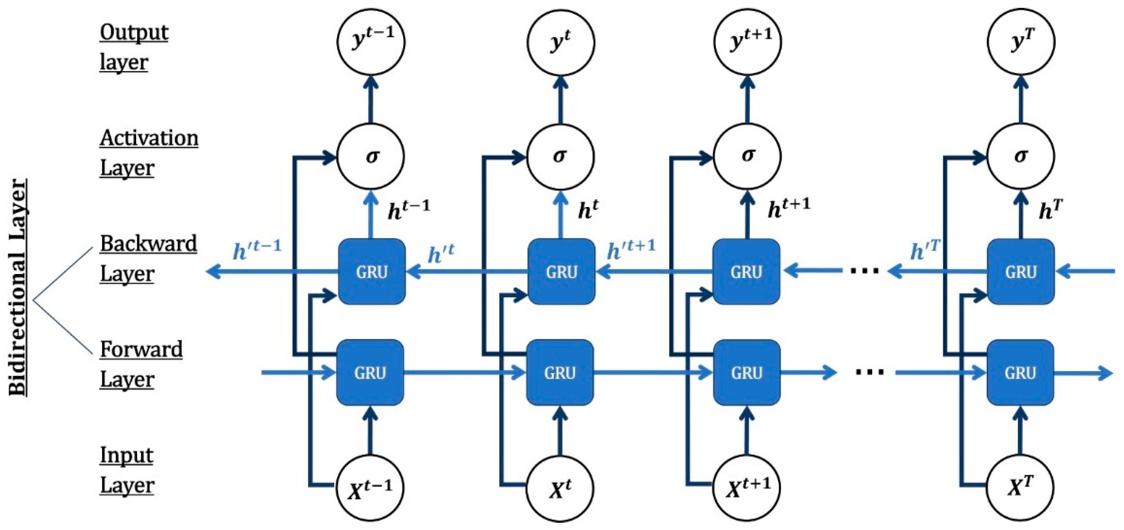
Figure 2. BGRU architecture.
Vibration 08 00070 g002
Figure 3. Bartec Syscom Rock Vibration unit.
Vibration 08 00070 g003
Figure 4. Time series of the studied projects. The project number and duration of vibration recording are shown for each project.
Vibration 08 00070 g004
Figure 5. Data windowing concept.
Vibration 08 00070 g005
Figure 6. First three data windows with input, label, and shift widths of 6, 1, and 1.
Vibration 08 00070 g006
Figure 7. Architecture of the neural network model.
Vibration 08 00070 g007
Figure 8. Training, validation, and test data prediction in project 1 with BGRU method.
Vibration 08 00070 g008
Figure 9. Prediction of the test data in project P1 using ARIMA, RF and BGRU.
Vibration 08 00070 g009
Figure 10. Prediction of the test data in project P2 using ARIMA, RF and BGRU.
Vibration 08 00070 g010
Figure 11. Prediction of the test data in project P3 using ARIMA, RF and BGRU.
Vibration 08 00070 g011
Figure 12. Prediction of the test data in project P4 using ARIMA, RF and BGRU.
Vibration 08 00070 g012
Figure 13. Prediction of the test data in project P5 using ARIMA, RF and BGRU.
Vibration 08 00070 g013
Figure 14. Prediction of the test data in project P6 using ARIMA, RF and BGRU.
Vibration 08 00070 g014
Figure 15. Prediction of the test data in project P7 using ARIMA, RF and BGRU.
Vibration 08 00070 g015
Figure 16. Prediction of the test data in project P8 using ARIMA, RF and BGRU.
Vibration 08 00070 g016
Figure 17. Prediction of the test data in project P9 using ARIMA, RF and BGRU.
Vibration 08 00070 g017
Figure 18. Prediction of the test data in project P10 using ARIMA, RF and BGRU.
Vibration 08 00070 g018
Figure 19. Prediction of the test data in project P11 using ARIMA, RF and BGRU.
Vibration 08 00070 g019
Figure 20. Prediction of the test data in project P12 using ARIMA, RF and BGRU.
Vibration 08 00070 g020
Table 1. Characteristics of projects where ground vibration is monitored.
Project No.Duration (Days)LocationNotes
189Basement slab in a neighboring two-story house.Events in the training data.
224On the existing ground, on the boundary of a construction site.Events in the whole data.
3121Basement slab in a neighboring two-story houseEvents in the training data.
448First floor slab in a neighboring convenience storeNo event. Peaks are observed in the whole data.
553Basement slab in a neighboring three-story industrial building.Events in the training data. Other peaks in the whole data.
641First floor slab in a neighboring one-story industrial building.Events in the whole data.
741Mounted on the midpoint of a wall in a neighboring one-story industrial buildingEvents in the training data. Some peaks in the testing data.
8330On the existing ground, on the boundary of a construction site.Events in the whole data.
9330Mounted on the midpoint of a wall in a neighboring multi-story residential buildingPeaks in the whole data.
1031Mounted on the midpoint of a wall in a neighboring church building towerVery small ambient vibration.
1115On the existing ground, on the boundary of a construction site.Peaks in the testing data.
12165First-floor slab in a neighboring one-story industrial building.Peaks in the training data.
Table 2. Characteristics of monitored projects, including equipment type, source distance, and construction purpose.
Project No.Dominant Construction EquipmentApproximate Distance to the SourceGeneral Construction Purpose
1Loaded trucks; Vibratory roller10–25 mTrail Extension
2Small bulldozer; Vibratory roller0–10 mTrail Extension
3Loaded trucks; Large bulldozer;
Hydraulic breaker
0–10 mExcavation; Foundation installation
4Loaded trucks; Jackhammer; Small bulldozer0–10 mExcavation; Grading
5Loaded trucks, Vibratory roller, Excavator0–10 mSite Remediation; Excavation; Backfilling
6Vibratory roller; Large bulldozer0–10 mExcavation; Building Construction
7Vibratory roller; Loaded trucks10–25 mExcavation; Building Construction
8Loaded trucks; Small and large bulldozer0–10 mExcavation; Foundation installation; Grading
9Loaded trucks; Small and large bulldozer10–25 mExcavation; Foundation installation; Grading
10Not explicitly defined25–50 mUnderground subway development
11Loaded trucks; Large bulldozer;
Hydraulic breaker
10–25 mExcavation; Foundation installation
12Loaded trucks; Large bulldozer;
Hydraulic breaker
0–10 mExcavation; Shoring, Foundation installation
Table 3. Construction vibrations thresholds based on Toronto Municipal Code.
f (Hz) P P V (mm/s)
f < 4 8
4 < f < 10 15
f > 10 25
Table 4. Optimal Random Forest hyperparameters.
Project No.Max DepthMin. Samples LeafMin. Samples Splitn_estimators
180518401
260189740
3None *1713319
460193781
5701718101
640108140
7None *410300
8601918791
9401213104
10100191849
1130118289
1210410300
* The nodes are enlarged until all leaves contain less than min_samples_split samples.
Table 5. Optimal ARIMA Parameters.
Project No.pqd
1211
2211
3112
4211
5112
6111
7211
8211
9112
10112
11112
12211
Table 6. Hyperparameters of the sequential model.
HyperparameterTuned Value
BGRU neuron numbers n 1 = 200 , n 2 = 100
Rate of dropout d 1 = 0.4 , d 2 = 0.4
Maximum number of epochs300
Patience for early stopping10
OptimizerAdam
Learning rate0.0001
Batch size48
Data window input length6
Data window label length1
Data window shift length1
Training split ratio0.7
Validation split ratio0.2
Testing split ratio0.1
Table 7. Prediction metrics for three methods BGRU, RF, and ARIMA.
Project No.BGRURFARIMA
R-SquaredRMSER-SquaredRMSER-SquaredRMSE
183.50.0015NG *0.048NG0.0192
298.80.128178.90.534885.40.4548
395.40.019751.90.064243.40.0695
499.80.015271.00.194183.10.1465
597.60.102346.10.496974.00.3410
699.00.142179.70.659988.10.4988
798.10.0933NG0.735884.80.2676
899.80.026953.50.411467.20.3450
999.50.010346.00.110964.90.0892
1099.30.000732.20.005657.90.0065
1194.50.28148.11.178168.90.6655
1299.80.008846.10.165964.40.1343
* NG means negative.
Disclaimer/Publisher’s Note: The statements, opinions and data contained in all publications are solely those of the individual author(s) and contributor(s) and not of MDPI and/or the editor(s). MDPI and/or the editor(s) disclaim responsibility for any injury to people or property resulting from any ideas, methods, instructions or products referred to in the content.