A Coupled Harmonic Balance-Based Approach for the Non-Linear Dynamics of Spur-Gear Pairs

Abstract

Noise, vibration and harshness analyses are of great interest for the latest developments of the gearboxes of electric vehicles. Gearboxes are now the main source of vibrations, since electric powertrains are much quieter than internal combustion engines. Traditionally, the simulation of the non-linear gear dynamics is studied by first performing a series of preliminary static analyses to compute the static transmission error (STE). The STE (i.e., in the form of varying mesh stiffness) is then accepted as the system’s excitation source to compute the dynamic transmission error (DTE). This paper presents a novel approach to analyze the non-linear dynamics of gears which does not require any preliminary static analyses. The method consists of a frequency–domain approach based on the Harmonic Balance Method (HBM) and the Alternating Frequency–Time (AFT) scheme, allowing for much faster simulations when compared to the widely used direct–time integration (DTI). The contact between the teeth is modeled as intermittent and penalty based with a varying gap. The time–varying gap between the teeth is initially approximated to a step function that guarantees the design contact ratio. The methodology introduced is tested on a lumped parameter model of a spur–gear pair already proposed and simulated in the literature. The results obtained with the novel approach are compared with the DTI simulation of the model as a reference. The excellent match between the different approaches validates the reliability of developed methodology.

1. Introduction

Gears serve as critical components in various mechanical systems, yet they are frequently subjected to issues such as vibrations. These vibrations are detrimental as they can induce damage, generate noise, and lead to malfunctions. The primary cause of vibrations in gears is the variation in contact stiffness, which fluctuates due to the changing number of teeth in contact during gear rotation [1].

The issue is well known and has been studied systematically since the mid 1800s with the early work of Walker, who proposed a coefficient relating the static and dynamic loads operating on gears as reported by [2]. In the last century, several lumped parameters models have been developed for the characterization of gear dynamics [3], addressing torsional vibrations [4] specifically teeth dynamics [1] and more in general geared rotor dynamics [5], where gears are often modeled as rigid disks with inertia on flexible shafts.

More recent studies that focused on torsional gear dynamics are still utilizing simple models for their analyses; Parker et al. [6] compared a single DOF model and a FE model in approximating the experimental dynamic response of a spur–gear pair, and Ambarisha and Parker [7] developed an analytical model able to capture the complex dynamics of a planetary gear when compared to its FE counterpart. In 2019, Dai et al. [8] proposed a hybrid analytical–computational approach that integrates the accurate FE static analyses with a compact lumped–parameters model that can both accurately simulate the torsional vibrations of the gears and correctly capture the stresses on the teeth.

However, even dynamic analyses on lumped parameter models can require significant computational time if they are performed by a time integration of the equation of motion of the system. The response of the gears is measured once steady state is reached; this requires performing the simulation of the initial transient until the response can be considered periodic. Trying to overcome the limitations of time integration, frequency–domain approaches were introduced in the field of gear dynamics. Harmonic Balance Method (HBM) allows for the determination of the steady–state response without having to solve for initial transient. HBM–based approaches significantly improve simulations times, but works on the fundamental assumption that the response to be computed must be periodic. Systems with clearance–type non–linearity (as gearing is) have shown to exhibit chaotic behaviors under specific operating conditions. Kahraman and Blankenship in [9] experimentally proved the existence of chaotic behavior testing different sets of gears under multiple loading conditions. However, non–periodic or quasi–periodic responses have been shown to appear mostly in simulation results. In fact, extensive studies have been performed on simplified gear models to characterize the impact of various parameters in the capability of gears to exhibit non–periodic or quasi–periodic responses. In this regard, early work was carried out by Kahraman and Singh in [10]; more recently, Huang et al. [11] have studied the effect of surface roughness in combination with backlash on spur gears, for example, and Molaie at al. [12] investigated chaotic behavior in spiral bevel gears using two different torsional lumped parameter models. In any case, the limitation of HBM–based approaches in addressing chaotic behaviors does not represent a significant step back, since industrials currently do not indulge in this type of analysis.

Some definitions are necessary for the following discussion in this paper. Transmission errors (TEs) are defined as the difference between the positions that perfectly rigid gears would occupy during ideal motion and the effective positions occupied by flexible gears. The static transmission error (STE) is typically defined as the TE obtained through a sequence of low–speed or quasi–static analyses on loaded gears [13]. The dynamic transmission error (DTE) is the counterpart of the STE when calculated at high rotational speeds. Instead of the STE, some prefer to introduce the concept of mesh stiffness (see [14] for a review on strategies to compute the mesh stiffness), which is related to the ratio of the torque applied to the gears and the STE. In practice, the STE and mesh stiffness provide similar information.

Commonly, the study of gear dynamics in the frequency domain is performed by first computing the STE (or the mesh stiffness function) and subsequently using it as a dynamic excitation to obtain the DTE [6,15,16]. This approach is the standard especially for frequency–domain approaches; in [17], a novel continuation method is proposed for the HBM solution of a lumped parameter model of a gear system, in their approach, the mesh stiffness is a preliminary requirement for the dynamic simulation. A similar approach is followed in [18] by Öztürk et al., where the loaded STE must be available prior to the HBM dynamic simulation in order to study planetary gear systems’ dynamics. In their paper, the effect of different profile modifications is assessed, and a different LSTE must be computed for the different models. Initially solving the system to obtain the STE can be cumbersome, especially for large systems; moreover, it represents an approximation because it assumes that the static (or quasi–static) solution of the system is not affected by the dynamics of the system. In the field of turbo–machinery, where HBM has been extensively applied, it has been proven that the uncoupled static–dynamic solution can lead to inaccurate results. Coupled HBM was developed to allow for accurate predictions of dynamic responses of non–linear models with friction damping. Zucca et al. [19] used coupled HBM with an Alternating Frequency–Time (AFT) on lumped parameter models with friction contact. They argue that considering the static and dynamic problem as uncoupled leads to inaccurate solution when compared to DTI simulations as a reference.

In this paper, the use of coupled HBM is extended to gear dynamics, developing a method capable of overcoming the differences between STE and DTE. The transmission error is obtained in a single analysis considering the coupling between the static solution and the dynamic one. The simulation algorithm is enabled by the use of the Alternating Frequency–Time (AFT) approach [20]. During the Newton–Raphson iteration to solve the non–linear set of equations expressed in the frequency domain, the AFT approach allows us to momentarily move to the time domain to compute the non–linear contact forces arising from the interaction between teeth pairs.

The methodology was implemented in a MATLAB (R2022b) script and the test system was solved, making use of a continuation method to guarantee convergence around turning points and unstable branches of the responses.

The following sections will focus on:

• In Section 2, Methodology, a comprehensive description of the proposed approach is presented, and details on the numerical solution strategy are also highlighted;
• In Section 3, Results and Discussion, comparative analyses are carried out on a simple lumped–parameter model. Non–linear dynamic analyses are performed with both DTI (reference) and the developed methodology.
• In Section 4, the final conclusions are drawn.

2. Methodology

The described approach is referred to as coupled HBM and has been introduced in [19] for systems with dry friction contacts. In this paper, the method is applied for the first time to gear dynamics. The most distinctive feature of gear systems, with respect to other components the coupled HBM method was applied to, is the existence of relative rigid body kinematics between the bodies in contact, which implied a two–step approach at the point at which HBM was implemented: (i) a set of quasi–static analyses to compute the STE of the gears; and (ii) a dynamic analysis to compute the DTE of the gears, using the STE as a periodic input. The advantages of CHBM in comparison with other solution methods can be found in [19]; however, it also provides several specific advantages to the gear–dynamics simulation framework when compared to the state of the art:

• No preliminary static analyses are required;
• No approximations/assumptions are required on the mesh stiffness;
• Suitable for the integration with different contact models.

The approach also presents some limitations:

• Because of the clearance type nonlinearities, several harmonics might be required to obtain a converged solution,
• The stiffness matrix can be singular for gear–dynamics problems, leading to bad conditioning of the dynamic stiffness and hard–to–obtain Newton–Raphson convergence;
• The basic assumption of the HBM must be valid, and the response to be computed must be periodic, meaning that gear’s chaotic behavior can be hardly studied with this approach.

2.1. Single DOF Model

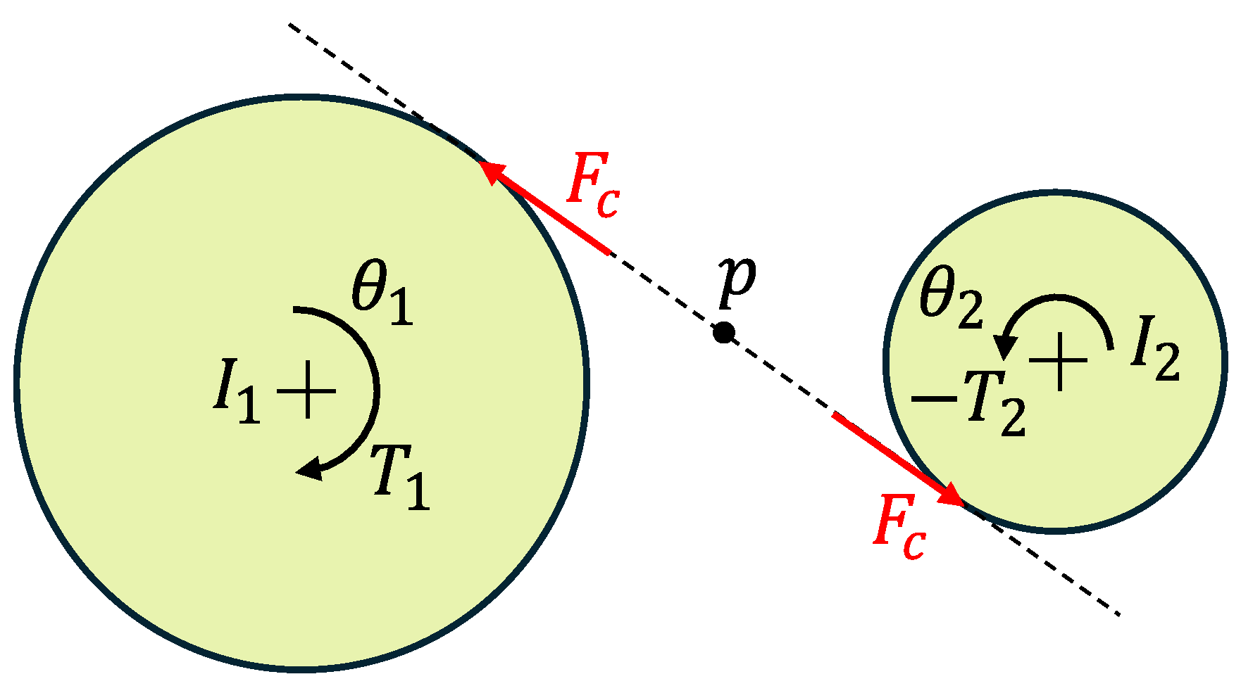
The demonstration of the applicability of the method is performed through the introduction of a simple, lumped–parameter model. The introduced one (see Figure 1) was already studied in [6], when trying to approximate some available experimental results.

The model is composed of two gears with $I_1$ and $I_2$ moments of inertia, $r_1$ and $r_2$ base radii, and $T_1$ and $T_2=T_1{r}_2/r_1$ torques applied to the gear. Given that no torsional stiffness or damping constrain the rotational DOF of the gears, the equations of motion can be written as

$$I_1{\ddot{\theta }}_1+F_c{r}_1=T_1$$

(1)

and

$$I_2{\ddot{\theta }}_2-F_c{r}_2=-T_1{r}_2/r_1.$$

(2)

From Equations (1) and (2), the following set of equations can be easily obtained:

$$I_2{I}_1{\ddot{\theta }}_1{r}_1+I_2{F}_c{r}_1^2=I_2{T}_1{r}_1,$$

(3)

$$I_1{I}_2{\ddot{\theta }}_2{r}_2+I_1{F}_c{r}_2^2=-I_1{T}_1{r}_2^2/r_1.$$

(4)

Subtracting Equation (3) from Equation (4), the following is obtained:

$$I_1{I}_2\left({\ddot{\theta }}_2{r}_2-{\ddot{\theta }}_1{r}_1\right)-F_c\left(I_1{r}_2^2+I_2{r}_1^2\right)=-T_1\left({\displaystyle \frac{I_1{r}_2^2}{r_1}}+I_2{r}_1\right),$$

(5)

which leads to:

$${\displaystyle \frac{I_1{I}_2}{I_1{r}_2^2+I_2{r}_1^2}}\left({\ddot{\theta }}_2{r}_2-{\ddot{\theta }}_1{r}_1\right)-F_c+T_1{\displaystyle \frac{{\displaystyle \frac{I_1{r}_2^2}{r_1}}+I_2{r}_1}{I_1{r}_2^2+I_2{r}_1^2}}=0.$$

(6)

Introducing the TE as the relative DOF between the gears $x={\theta }_2{r}_2-{\theta }_1{r}_1$ and introducing a damping term proportional to $\dot{x}$, the equation of motion becomes:

$${\displaystyle \frac{I_1{I}_2}{I_1{r}_2^2+I_2{r}_1^2}}\ddot{x}+C\dot{x}-F_c+T_1{\displaystyle \frac{{\displaystyle \frac{I_1{r}_2^2}{r_1}}+I_2{r}_1}{I_1{r}_2^2+I_2{r}_1^2}}=0,$$

(7)

or, in the more compact form:

$$M\ddot{x}+C\dot{x}-F_c+F_{ext}=0.$$

(8)

The external excitation is collected in the $F_{ext}$ term; it is directly dependent on the torque $T_1$ applied to the first gear. The external excitation is generally a periodic function known a priori.

$F_c$ is the contact force being exchanged between the teeth of the gears. In the most general case, $F_c$ is a non–linear function of time (t), the transmission error (x), and its derivative ($\dot{x}$).

Considering the gears rotating at a constant angular speed ${\omega }^{\prime }$, once a steady state is reached, every point of the gears will occupy the same position after a $T^{\prime }=2\pi /{\omega }^{\prime }$ time period. However, considering the geometrical periodicity of the gears, the gears are already in an equivalent position after a period of $T=2\pi /z{\omega }^{\prime }$, with z the number of teeth. Consequently, the contact forces are also periodic with the same period T, and the effective pulsation of the system is $\omega =z{\omega }^{\prime }$.

The displacement and forces in Equation (8) can be expressed as a Fourier series:

$$x\left(t\right)=\sum _{h=0}^H{\tilde{x}}_h{e}^{jh\omega t},$$

(9)

$$F_{ext}\left(t\right)=\sum _{h=0}^H{\tilde{F}}_{ext,h}{e}^{jh\omega t},$$

(10)

$$F_c\left(t,x,\dot{x}\right)=\sum _{h=0}^H{\tilde{F}}_{c,h}{e}^{jh\omega t}.$$

(11)

The quantities ${\tilde{x}}_h$, ${\tilde{F}}_{ext,h}$, and ${\tilde{F}}_{c,h}$ are the complex Fourier coefficients associated with the $h^{th}$ order; j is the imaginary unit. The series are truncated at an arbitrary order H.

Equations (9)–(11) are substituted in Equation (8) and the HBM is enforced. The equation for a generic order h is:

$$\left(-h^2{\omega }^{2}M+jh\omega C\right){\tilde{x}}_h-{\tilde{F}}_{c,h}+{\tilde{F}}_{ext,h}=0.$$

(12)

The set of algebraic equations for all the harmonic orders are collected in the expression:

$$\left[D\left(\omega \right)\right]\left\{\tilde{X}\right\}-\left\{{\tilde{F}}_c\right\}+\left\{{\tilde{F}}_{ext}\right\}=\left\{0\right\},$$

(13)

where $\left[D\left(\omega \right)\right]$ is the dynamic stiffness.

The generic model presented in Figure 1 can be simulated using direct time integration (DTI) solving Equation (8) or it can be solved in its frequency–domain expression (Equation (13)) using non–linear solution methods (e.g., Newton–Raphson) with an Alternating Frequency–Time scheme (AFT) [20].

The AFT scheme starts from a given estimation value of the Fourier coefficients of the generalized displacements ${\left\{\tilde{X}\right\}}^{*}$. The displacements are then expressed in time domain over a single period via the Inverse Fast Fourier Transform (IFFT). The contact model allows us to obtain the contact force evolution over time given the evolution of the generalized displacements. The sequence of generalized contact forces is eventually expressed back in the frequency domain via the Fast Fourier Transform (FFT), thus obtaining the Fourier coefficients of the contact forces ${\tilde{F}}_{c,h}$ for the different harmonics retained in the HBM. The Fourier coefficients of the contact force, deriving from the guessed solution ${\left\{\tilde{X}\right\}}^{*}$ are collected in the vector ${\left\{{\tilde{F}}_c\right\}}^{*}$.

If the residual of the equation of motion is still too large, a new estimation of the Fourier coefficient of the generalized displacements must be provided. The iterations proceed until the residual of the equation of motion can be considered sufficiently small, and once convergence is reached, the process is repeated for a different excitation frequency (or rotational speed). The whole process is summarized in Figure 2.

2.2. Contact Model

A contact model is required to express $F_c$ as a function of time $\left(t\right)$, the transmission error $\left(x\right)$ and its derivative $\left(\dot{x}\right)$. This model can then be used as is in the different formulations of the problem (time domain or frequency domain).

In the literature, multiple contact models have been introduced to mimic the dynamics of spur gears. Özguvent et al. describe the most common ones in [3]. The contact models used in the literature for other lumped–parameter models of spur gears require an excitation source computed via preliminary quasi–static analyses. Generally, the excitation sources considered are a time–varying mesh stiffness, a displacement error in the gear meshing, or a combination of the two. In [6,21,22], for example, the model is excited through a varying mesh stiffness function, so an explicit time expression of the equivalent contact stiffness must be computed prior to the dynamic analyses. In [13,17,23] the contact models include an excitation source from transmission errors that, again, must be computed in advance.

The main advantage of the introduction of the coupled HBM being the solution of the static and dynamic problem simultaneously, requires the introduction of a slightly different contact model, one that only requires the knowledge of the kinematics of the gears.

Considering the rigid rotation and mating of the gears, the contact ratio $c_r>1$ defines the average number of teeth in contact during a period of the motion. The varying number of teeth in contact leads to changes in the equivalent stiffness of the contact which represent the source of dynamic excitation in the studied model. Moreover, the vibrations induced by this phenomenon can lead the teeth on opposing gear to close or open the contact in a different instant than the rigid case. The proposed contact model wants to mimic this behavior.

The basic idea is that, during one period of the rigid rotation of the gears a couple of teeth will be either in contact or not. The contact status (open or close) depends on the relative distance between the teeth. This distance is referred to as gap. In this scenario, the gap is not representative of the backlash, but it is the distance between the teeth on the active flank; this distance periodically varies going to zero when contact occurs.

The gap between two teeth can be either zero or a positive value. The relative position of the contact points $x={\theta }_2\left(t\right)r_2-{\theta }_1\left(t\right)r_1$ is positive if they tend to separate and negative if they tend to interpenetrate. A clearance type contact is defined in the form of

$$\left\{\begin{array}{cc}{F}_c\left(t\right)=-k_c\left(x\left(t\right)+\mathit{gap}\left(t\right)\right)\hfill & \mathrm{if}x+\mathit{gap}<0\hfill \\ F_c\left(t\right)=0\hfill & \mathrm{if}x+\mathit{gap}\ge 0\hfill \end{array}\right.$$

(14)

where $k_c$ is the contact stiffness. The contact status is fully dependent on the total relative position of the contact at every time step. This contact model allows the system to find an equilibrium considering both the static and dynamic components of the response.

Considering a model with contact ratio $c_r=1.75$, during one (rigid) rotation period of the gears, three couples of teeth will be in contact with each other at a certain point. Considering the representation in Figure 3, the central couple of teeth will be in contact for the entire rotation period, the high couple of teeth will start as separated and will enter contact after some time. On the contrary, the low couple of teeth will start in contact and will separate as the rotation continues.

To consider the interactions between the teeth described, the system presented in Figure 1 is completed in Figure 4, including three contact elements representing the couples of teeth.

The gap operating in the different contact elements will vary over time. As a first approximation, a step function is introduced (Figure 5); the gap for all the teeth is set to 0 when the teeth are in contact, and to 1 when they are open. The gap jumps are highlighted by the arrows and are set to enforce the design contact ratio. The approximation of the gap variation as a step function is not representative of the real behavior of the teeth contact; the results obtained with this model will not be quantitatively close to any experimental results possibly available. However, since the scope of this paper is to show the applicability of the coupled HBM to the simulation of gear dynamics, having an accurate contact model is not a requirement. In future work, effort will be put into this aspect to improve the quality of the results and to investigate the applicability of the methodology to more representative models.

3. Results and Discussion

The model considered for the following analyses considers a couple of identical gears. The Equation (7) can then be simplified as follows:

$${\displaystyle \frac{I}{2r^2}}\ddot{x}+C\dot{x}-F_c+T{\displaystyle \frac{1}{r}}=0,$$

(15)

where the parameters considered are collected in

Table 1. System parameters.

I (Kg/m2)	r (m)	C (Ns/m)	z	${\mathit{c}}_{\mathit{r}}$	$\mathit{\phi }$	${\mathit{k}}_{\mathit{c}}$ (N/m)
0.0158	0.0705	4038.2	50	1.75	20°	2.6 × 108

. In the table, the quantities are I the moment of inertia, r the base radius, and z the number of teeth for a single gear, while C is the total damping of the system, $c_r$ the contact ratio, $\phi$ the pressure angle, and $k_c$ the contact stiffness for a single teeth pair.

To validate the methodology proposed, the reference results are obtained by a direct time integration of the system expressed in Equation (15). The solutions are obtained by implementing the Newmark method as a MATLAB (R2022b) algorithm with $\beta =0.5$ and $\gamma =0.25$ [24]. The simulation is carried out until a steady state is reached.

3.1. Non–Linear Forced Responses

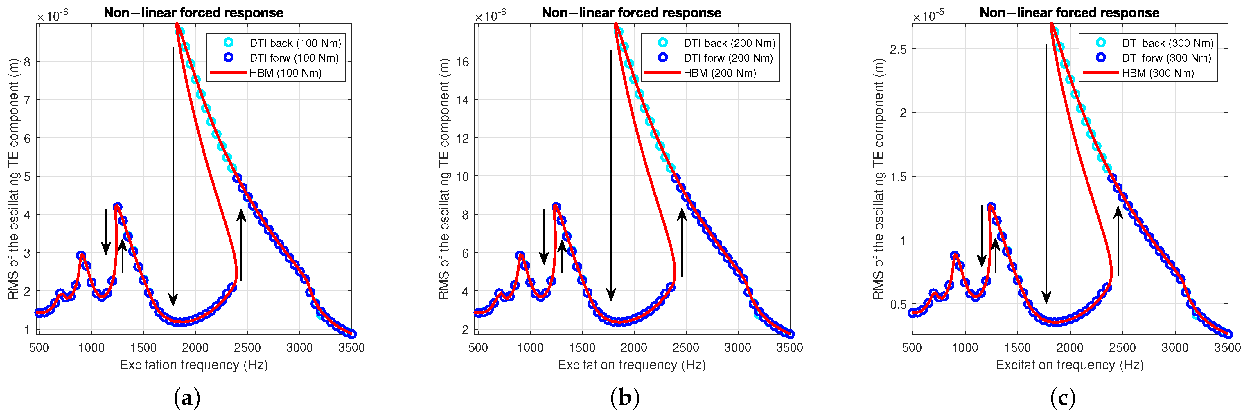
Different analyses are performed for multiple levels of constant torques (T) applied, namely 100 Nm, 200 Nm, and 300 Nm. The number of harmonics considered in the MHBM solution is $H=14$. Since the system has only one degree of freedom (DOF), it is possible to simulate it using a large number of harmonics, although good results could be obtained by retaining fewer harmonics. It was also intention of the authors to properly capture the contact force behavior, considering that the unrealistic step–gap function induces instant changes in the contact status leading to steep gradients of the contact stiffness during the rotation of the gears.

In Figure 6, the non–linear forced responses of the system are presented; the jumps phenomena are highlighted by black arrows. The HBM simulations are performed by implementing a continuation method; however, to obtain the unstable branches of the response, the scaling of the equations of motion and a careful tuning of the continuation step control logic is necessary. The DTI simulations are carried out, starting from the lowest frequency of the range (forward, forw) and from the highest as well (backward, back).

The different simulation methods are in excellent agreement with each other. All the peaks are predicted accurately both in terms of amplitude and frequency. The jump phenomena typical for this kind of systems are predicted accurately by the HBM simulations.

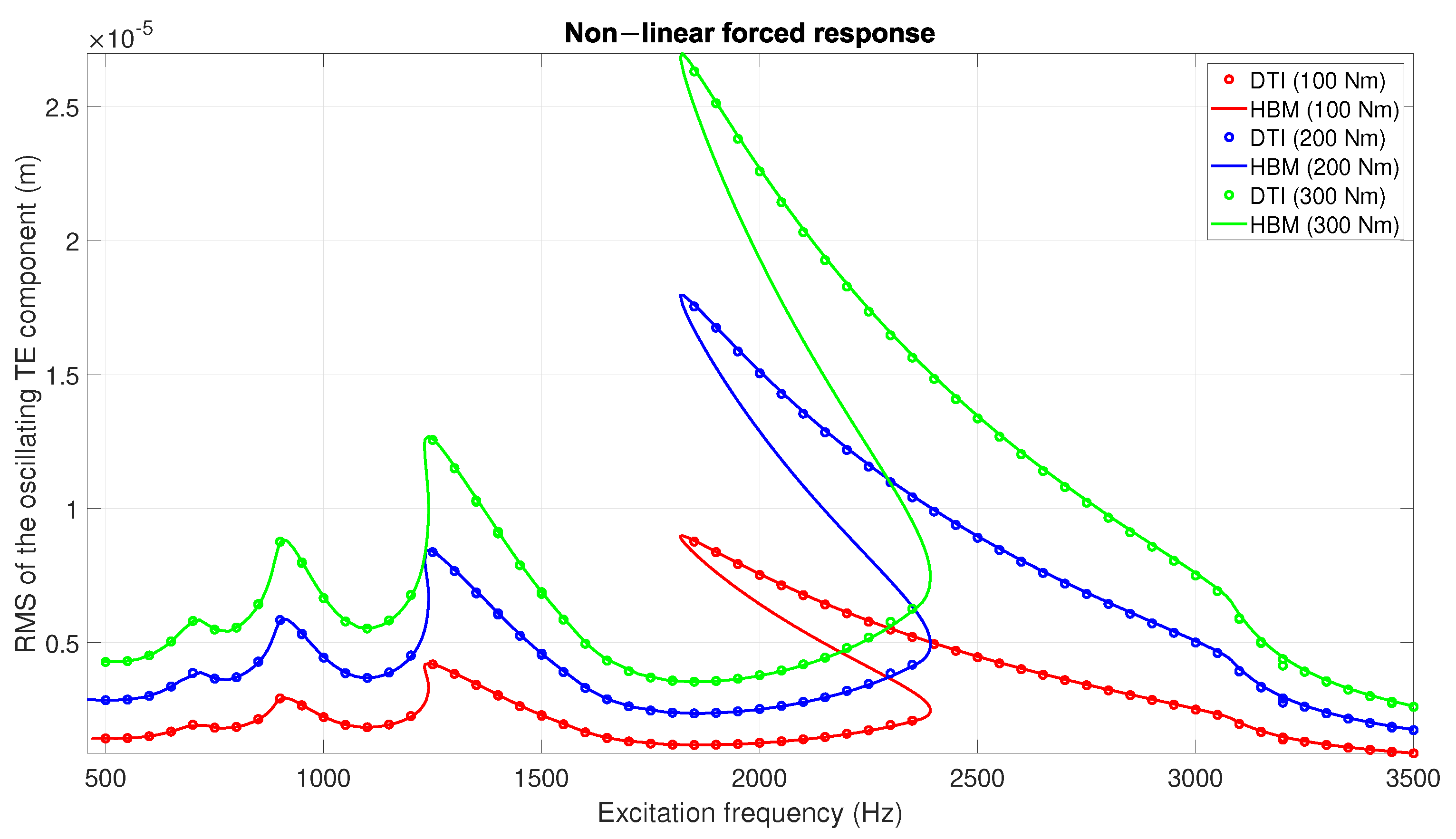
In Figure 7, a comparison of the non–linear forced responses is presented. It is worth noting that the different responses seem to be scaling linearly with the constant torque applied. This effect is not present in more accurate simulations or in the experimental results available in the literature [6,25]. Typically, the increase in the constant torque level tends to “linearize” the system, resulting in less softened peaks. In fact, high levels of constant torque counters the complete separation of the teeth at excitation frequencies close to resonance.

The presented system does not completely capture this behavior as a consequence of the simplified contact modeling. The gap approximated to a square function with a harsh difference between the closed and open status does not allow for a refined tracking of the limits of the section of the response curve in separation. In reality, the gap between the teeth varies regularly as a consequence of the gears’ kinematics. More realistic contact modeling will be introduced in future work, to both improve the convergence of the solution method and increase the accuracy of the results obtained with respect to experimental results available in the literature.

3.2. Contact Force

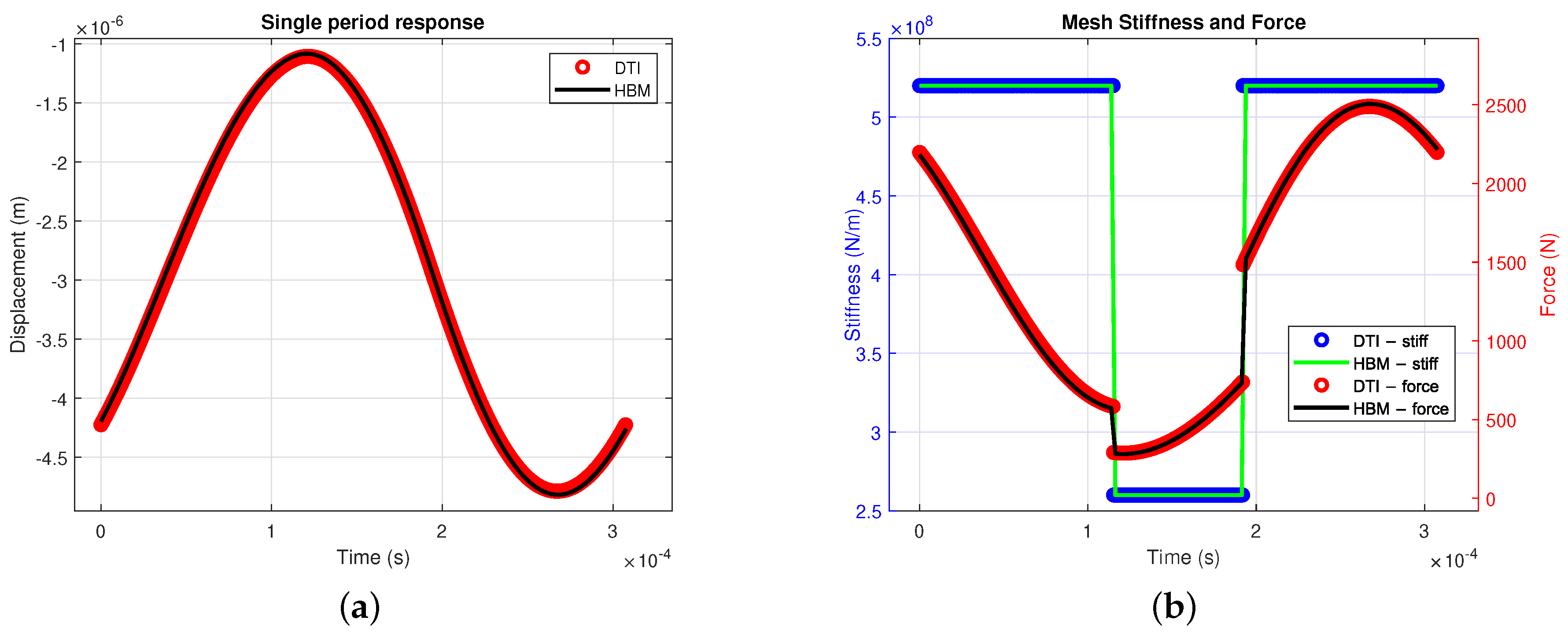
In this sub–section, a specific focus on the contact quantities is presented. The accuracy of the proposed methodology is assessed by comparison of the contact force and equivalent contact stiffness in the HBM and DTI simulations. The following comparisons are performed for the case with $T=100$ Nm constant torque applied, but equivalent results were obtained for the other cases.

In Figure 7, the plots associated with an excitation frequency of 3250 Hz are presented. Being relatively far from the resonances, the response at regime for a single period is close to a sinusoidal signal (on the left). The simulation carried out with the proposed methodology (HBM) and with the time integration (DTI) are in very good agreement. On the right side, the computed contact force is presented; the steep changes are associated with the gap jumps shown in Figure 5. The instantaneous ratio between the contact force and the response is defined as the mesh stiffness, this quantity is plotted associated with the contact force. The mesh stiffness for this case is a step function that varies between $k_c$ and $2k_c$, giving an indication on the number of contact elements (see Figure 4) operating at each time step. Both the mesh stiffness and the contact force are simulated remarkably well by the HBM solution method when compared to the DTI standard approach.

The same comparisons are presented for other significant excitation frequencies; in Figure 8, the focus is on 1250 Hz. Specifically, at the resonance frequency of the first super–harmonic, the displacement response presents two peaks. The mesh stiffness obtained for this excitation frequency shows three distinguished levels; for some time steps, the stiffness is zero, which means that the two gears are completely separated and they are not exchanging any force. This effect is given by the dynamics of the system that is producing vibration levels high enough to open the contact.

In Figure 9 and Figure 10, the results at the main resonance’s frequency are presented. At this frequency, two stable results are possible; the response with the highest amplitude is presented in Figure 9, while the one with the lowest amplitude is presented in Figure 10. The response in Figure 9 is mainly mono–harmonic; the contact force reaches the highest values of the frequency range and, for a significant portion of the period, separation occurs. While, in Figure 10, the response shows a non–neglectable contribution of the second harmonic. The mesh stiffness has again assumed the form it has far from resonance (as in Figure 11), but in this case the contact force signal presents two peaks, given that the excitation frequency of interest is closer to the first super–harmonic.

4. Conclusions

A new approach to the analyses of spur–gear pairs is presented in this paper. The already well–established Harmonic Balance Method in its coupled static–dynamic formulation is extended to gears’ dynamic problems, where, in contrast to other problems previously solved with the CHBM, relatively rigid body kinematics between the bodies in contact is present. A solution scheme is proposed, making use of the Alternating Frequency–Time method. The AFT method allows us to compute the non–linear contact forces moving temporarily to the time domain via a IFFT of the generalized displacements. Subsequently, the Fourier coefficient of the contact forces are obtained with the FFT of the single period time signal of the contact forces.

A contact model is required to express the contact force as a function of the generalized displacements and its derivative. A penalty–based contact model is introduced, defining a time–varying gap between the teeth.

The formulation obtained allows us (under the basic assumption of the HBM) to simulate the system in the frequency domain without the need for any preliminary static analysis or assumptions on the mesh stiffness function.

In the Section 3, multiple non–linear responses are presented, comparing the responses amplitudes obtained with the Newmark method and with the proposed methodology. The comparison holds for all the frequency range considered.

Contact force, mesh stiffness, and one period responses are also compared at specific frequencies. HBM and DTI show overlapping results for all the cases.

Coupled HBM proved to be an effective alternative to DTI for the simulation of simple lumped–parameter models.

The proposed methodology allows for the incorporation of various contact models without affecting the overall framework. The authors plan to leverage this flexibility in future work by introducing more realistic contact models to enhance the accuracy of the simple lumped–parameter model in relation to actual spur–gear pairs.