Article

Fault Classification in Diesel Engines Based on Time-Domain Responses through Signal Processing and Convolutional Neural Network

by
Gabriel Hasmann Freire Moraes
,
Ronny Francis Ribeiro Junior
and
Guilherme Ferreira Gomes
*
Mechanical Engineering Institute, Universidade Federal de Itajuba (UNIFEI), Itajuba 37500-903, Brazil
*
Author to whom correspondence should be addressed.
Vibration 2024, 7(4), 863-893; https://doi.org/10.3390/vibration7040046
Submission received: 30 July 2024 / Revised: 3 September 2024 / Accepted: 27 September 2024 / Published: 29 September 2024
(This article belongs to the Special Issue Vibration Damping)

Abstract

:
In today’s interconnected industrial landscape, the ability to predict and monitor the operational status of equipment is crucial for maintaining efficiency and safety. Diesel engines, which are integral to numerous industrial applications, require reliable fault detection mechanisms to reduce operational costs, prevent unplanned downtime, and extend equipment lifespan. Traditional anomaly detection methods, such as thermometry, wear indicators, and radiography, often necessitate significant expertise, involve costly equipment shutdowns, and are limited by high usage costs and accessibility. Addressing these challenges, this study introduces a novel approach for fault detection in diesel engines by analyzing torsional vibration data in the time domain. The proposed method leverages short-term Fourier transform (STFT) and continuous wavelet transform (CWT) techniques, integrated with a convolutional neural network (CNN) to identify hidden patterns and diagnose engine conditions accurately. The method achieved a detection accuracy of 96.5% with STFT and 92.2% with CWT. To ensure robustness, the model was tested under various noise conditions, maintaining accuracies above 70% for noise levels up to 40%. This research provides a practical and efficient solution for real-time fault detection in diesel engines, offering a significant improvement over traditional methods in terms of cost, accessibility, and ease of implementation.

1. Introduction

Despite the advent of electrification culture, internal combustion engines continue to hold immeasurable importance in global industrial, economic, and social development. They are found at various levels, including public transportation, industrial machinery, electric generators in hospitals as backup during power outages, and more. Given their significance, ensuring the correct operation of these engines is essential to guarantee the availability and safety of the systems in which they are installed.
In this context, it is crucial to identify any abnormal operating conditions as early as possible to prevent them from escalating into serious failures, leading to larger problems such as poor performance or equipment breakdown. Various methods already exist for identifying such conditions, ranging from simple non-destructive testing procedures like liquid penetrant and magnetic particle testing to more complex methods such as ultrasound, radiography, and thermography ([1]). However, these methods typically require advanced knowledge in signal reading and deep technical understanding, making them expensive and sometimes challenging to access.
However, despite the availability of numerous diagnostic methods, significant challenges remain in terms of accessibility, expertise required, and the limitations associated with traditional approaches. For instance, methods such as thermometry and ultrasound testing, while effective, demand substantial technical knowledge and often necessitate a complete shutdown of the equipment, leading to productivity losses. Additionally, the high costs and complexity of some methods limit their widespread adoption in various industrial settings. Furthermore, the application of support vector machines (SVMs) and Bayesian networks (BNs) in fault detection, although promising, is often constrained by their computational limitations and the need for feature extraction to be performed manually.
Given these shortcomings, there is a clear need for more accessible, cost-effective, and efficient diagnostic tools that can be applied in real-time without extensive technical requirements. The proposed methodology in this paper, which leverages convolutional neural networks (CNNs) in conjunction with signal processing techniques such as short-time Fourier transform (STFT) and continuous wavelet transform (CWT), aims to fill these gaps by providing a robust and automated approach to fault detection in diesel engines. This approach not only reduces the need for specialized knowledge but also offers faster execution with low computational demands, making it suitable for a wide range of industrial applications.
Therefore, new approaches using artificial intelligence have emerged, demonstrating excellent performance in various applications. Until a few years ago, methods like support vector machines (SVM) and Bayesian networks (BN) emerged as classifiers with good performance and low computational power requirements ([2]). It was only with the introduction of the AlexNET network that convolutional neural networks (CNNs) started to be more widely used, advancing in parallel with improvements in computational power. This type of deep learning (DL) has proven to be excellent for pattern detection in numerous fields, including fault classification and detection in engines.
Alongside the use of CNNs, signal pre-processing methods are often employed using tools such as short-time Fourier transform (STFT) or continuous wavelet transform (CWT) ([3,4,5]). These techniques enhance feature extraction for the studied problems and have generally proven effective in fault classification, even in combustion engines.
This paper presents a methodology for identifying and classifying certain types of faults in a marine diesel engine using simulated torsional vibration data from the crankshaft. Initially, these data are processed using time-frequency domain signal analysis techniques, employing short-time Fourier transform and continuous wavelet transform. Subsequently, the processed data are input into a convolutional neural network, which outputs the type of fault in the evaluated case. The study also analyzes the effect of adding noise to the signal on the classification performance of the proposed network. The methodology aims to demonstrate high accuracy in fault classification, paving the way for testing and real-world application, offering a solution with low computational demand and fast execution compared to currently used methods.
In an industrial landscape characterized by increasing interconnection and a quest for efficiency, anticipating faults in diesel engines becomes a critical component to ensure operational continuity and process effectiveness. The widespread use of these engines across various industrial sectors underscores the strategic importance of developing innovative methods for early anomaly detection. This study’s proposal to employ simulated rotational acceleration data, transformed through techniques like STFT and wavelet, to feed a convolutional neural network (CNN) responds to this demand.
The choice of simulated data was made based on the difficulty of accessing comprehensive real datasets and the need to create controlled environments for validation. Simulating faults in diesel engines can be costly and pose a risk to the engine’s integrity. The use of simulated and manufacturer-validated data allows for investigating the model’s viability without significant investments. Applying these transformations and using a CNN aims to overcome the limitations of traditional diagnostic methods, offering a faster, simpler, economically viable, and effective approach to identifying faults in diesel engines.
Furthermore, given the vast variety and complexity of existing engine models today, the described procedure aims to develop a globally applicable fault recognition method, independent of the embedded technology and proprietary nature of each equipment. Thus, this research is justified by its contribution to operational efficiency, safety, and sustainability in industries, proposing an innovative solution that integrates advances in signal processing and machine learning to enhance the reliability of engines in critical industrial environments.
The objective of this work is to use CNNs in conjunction with STFT and wavelet signal transforms to identify abnormal operating conditions (severities) in combustion engines through their vibration response.

State of the Art

Given the paramount importance of diesel engines in various industries, numerous studies have been conducted in recent years to investigate fault diagnosis methods in combustion engines and related machinery using various approaches.
In [6], the authors propose a method for analyzing faults in gasoline engines using the spark plug as the combustion sensor. This technique, called spark voltage characterization (SVC), is based on another method called ionic current monitoring system (ICMS) but eliminates external voltage sources and additional components. In this method, the waveform of the voltage applied to the spark plug during the ignition process is analyzed, and the efficiency of multilayer perceptron neural networks (MLPs) is investigated in classifying types of faults and anomalies in the combustion process with an accuracy of approximately 95%.
In [3], the authors study the efficiency of using wavelet transforms, specifically the continuous wavelet transforms and the wavelet packet transform, in detecting faults in transient regimes in rotating machinery, comparing it with FFT and STFT analyses. The faults, such as periodic rotor friction against the housing caused by imbalance and misalignment of the shafts, are analyzed under conditions of rapid acceleration/start-up and deceleration (no load applied by the engine). Vibration signals are obtained using proximity sensors and strain gauges, with accelerometers used for comparison. The study shows that the wavelet analysis outperforms the Fourier transform in transient regimes, with wavelet packet transform generating better spectral analysis than continuous wavelet transforms.
In [7], the authors use sound data from an internal combustion engine, employing an extension neural network (ENN) to detect and classify faults, such as air leakage into the engine intake, combustion failure in one or two cylinders, temperature sensor failure, and mass flow sensor failure. Fractal modulation wavelet analysis (wavelet packet decomposition, WPD) is used for feature extraction to feed the ENN, which consists of only an input layer and an output layer, achieving classification accuracy above 85%.
In [4], the authors evaluate the application of CNNs to detect seven different conditions (one normal and six faults) and extract features from (a) planetary reduction gearboxes through experimentation and (b) vibration data from a gearbox in public databases. Both raw datasets undergo fast Fourier transform (FFT). In case (b), data are collected from accelerometers attached to a reduction gearbox undergoing various faults for information gathering. The study compares various network configurations, highlighting a network with one convolutional layer, one pooling layer, and one fully connected layer with softmax activation as having the highest accuracy, achieving accuracy above 98% in detecting proposed faults in both cases.
In [8], the authors present a classification method for scramjet engine combustion modes based on convolutional neural networks. Static pressure data within the engine combustion chamber obtained through experimentation is evaluated by CNN in two ways: with raw signals and with a database of statistical features in the time and frequency domains (processed by FFT) generated from raw data. The results show that the CNN-based method can reveal characteristic information and classify the suggested scramjet engine combustion modes with an accuracy above 90%, outperforming other commonly used neural network types.
In [9], the authors propose a CNN-based method to estimate wear levels in bearings for each element, namely inner race, outer race, and ball. Notably, experimental vibrational data are automatically labeled using a combination of root-mean-square (RMS) and Shannon entropy, along with k-means clustering for data grouping. The data are converted into time-domain images for two-dimensional identification. The CNN, with three convolutional layers, achieves accuracy above 98% in fault identification.
In addition to convolutional neural networks (CNNs), recurrent neural networks (RNNs), particularly long short-term memory (LSTM) networks, have shown promise in fault diagnosis, especially for time series data. In [10], the authors proposed a physics-informed hyperparameter selection strategy for LSTM networks to enhance fault detection in gearboxes. By focusing on maximizing the discrepancy between healthy and faulty states, this method improved the detectability of subtle faults like gear tooth cracks and wear. This highlights the potential of LSTM networks in fault diagnosis, complementing CNN-based approaches by offering robust solutions in scenarios where temporal data patterns are critical.
Using two techniques with different data, Ref. [11] assesses the detection of faults in fuel misfire events in a four-cylinder, four-stroke gasoline engine. Vibration data acquired from accelerometers installed in the middle of the engine block and sound signals obtained from microphones positioned 30 cm from the equipment are simultaneously collected. In both techniques, spark plugs were removed from each cylinder one at a time to simulate faults, along with normal operating data, resulting in five different cases. The signals undergo FFT processing and feed an artificial neural network (ANN). The study demonstrates 99.30% accuracy for vibration signals and 98.7% accuracy for sound signals in identifying proposed classes.
Recent advancements in machine learning have introduced innovative approaches in fault diagnosis, particularly in complex industrial environments. Digital twin-driven assessments are becoming crucial for real-time gear surface degradation monitoring, enhancing predictive maintenance. Vibration-based gear wear monitoring and prediction techniques also benefit from integrating machine learning with traditional signal processing methods. Additionally, the physics-informed residual network (PIResNet) represents a significant breakthrough in bearing fault diagnostics. As proposed by [12], PIResNet incorporates physical laws into the neural network architecture, ensuring accurate and physically consistent diagnostics even under varying operational conditions. These emerging methods underscore the need for more adaptive and reliable fault detection solutions in industrial applications.
Equally important, Ref. [13] aims to expand the analysis of electric motors to other types of faults that may occur in these devices, such as motor base clearance, misalignment, and fractured bars and shafts. Acceleration signals obtained by uniaxial accelerometers are converted into time-frequency domain images using STFT, which are then utilized by the CNN. The network, with three convolutional layers and three pooling layers, achieves 100% accuracy in identifying the seven studied conditions, demonstrating excellent robustness of the proposed method.
New trends in fault diagnosis have explored various texture representation techniques, offering enhanced feature extraction capabilities for machine condition monitoring. For instance, Ref. [14] proposed a reliable fault classification method for induction motors using two-dimensional (2D) texture features combined with a multiclass support vector machine (MCSVM). This method converts time-domain vibration signals into 2D gray images, extracting texture patterns that are then used for fault classification, achieving remarkable accuracy even in noisy environments.
Another study [15] introduced a hybrid deep-transfer learning architecture that utilizes the Hilbert transform and a combination of deep convolutional neural networks (DCNNs) and long short-term memory (LSTM) layers. This approach effectively handles the non-linear and non-stationary nature of time-series fault data by extracting both temporal and spatial features from 2D images, resulting in superior fault detection accuracy across various datasets. These studies highlight the potential of advanced texture representation techniques in improving fault diagnosis, particularly in industrial applications. In this context, our research compares the performance of STFT and CWT with other emerging methods such as gammatone, EMD-gammatone, Hilbert transform, and segmentation techniques. This comparison aims to evaluate the effectiveness of different signal-processing approaches in capturing discriminative fault features, thereby enhancing the reliability and accuracy of fault diagnosis in diesel engines.
In [16], on the other hand, the authors apply a similar idea to combustion engines, using a magnetic pick-up sensor to capture the crankshaft’s rotational speed. They suggest applying a 1D CNN for real-time analysis of faults related to irregular fuel burning and changes in load conditions during engine operation. Feature extraction and fault classification are performed by a CNN with one hidden layer, achieving 99% accuracy in detecting abnormal operating conditions with low generalization error, showcasing good efficiency even for a simple network.
In [17], the authors analyze torsional vibration signals in a diesel engine for four different operating conditions, including one normal and three failure modes. Using artificial neural network and random forest methods, they classify and regress data from a simulated database with 3500 test points divided among the four conditions. Between the two methods, random forest achieves the lowest root mean square error (RMSE) and the lowest dispersion among values.
It is evident that there are few references in the literature that address more complex faults beyond the structural spectrum of the engine. Therefore, this study’s main objective is to develop a robust and effective methodology to classify different operating conditions (faults), including fuel supply failure, cylinder pressure drop, and air pressure drop at the engine intake, going beyond the extensively studied (mostly structural) faults in diesel engines using torsional crankshaft vibration signals. To achieve this, signal preprocessing techniques (STFT and CWT) will be applied to generate images in the time and frequency domains, which will be used in an artificial intelligence algorithm (CNN) to recognize new fault patterns.

2. Theoretical Background

2.1. Short-Time Fourier Transform

The Fourier transform is a fundamental mathematical technique that plays a crucial role in the analysis of signals and systems in various fields, such as engineering, physics, applied mathematics, signal processing, among others. The main idea behind it is to decompose a complex function or signal in the time domain into its frequency components. In other words, it allows for representing a signal as a sum (or integral, in the case of the continuous Fourier Transform) of sine and cosine functions with different frequencies. This is particularly useful because it is often easier to analyze and understand the behavior of a signal in the frequency domain than in the time domain.
This mathematical tool converts a function in the time domain f(t) into a function in the frequency domain F(ω), where ω represents the angular frequency of the wave. The formula for this transform for a given function in the time domain is calculated with Equation (1) ([18]):
f ^ ω = F f x = f x e i ω x d x
Its inverse, allowing one to obtain the function f(t) given its transform, is calculated with Equation (2):
f x = F 1 f ^ ω = 1 2 π f ^ ω e i ω x d ω
The short-time Fourier transform (STFT), also known as the Gabor transform, is an extension of the Fourier transform that can provide information about the temporal evolution of frequencies in a signal, i.e., how signals are positioned over time. While the traditional Fourier transform provides a global representation of frequencies across the entire signal, the STFT divides the signal into smaller segments and applies the Fourier transform to each individual segment. This approach provides a time and frequency representation given by a spectrogram, allowing the analysis of how the spectral characteristics of a signal vary over time. The formula for the STFT is calculated with Equation (3):
G ( f ) ( t ,   ω ) = f g ^ 1 t ,   ω = f τ e i ω x g ^ τ t d τ
where g t ,   ω τ is defined as follows:
g t ,   ω τ = e i ω τ g ( τ t )
The function g(t) is the kernel and is in general a Gaussian function calculated with the following Equation:
g t = e t τ 2 a 2
In Equation (5), a represents half the length of the window or segment over which the signal is analyzed, and the traditional Fourier transform is applied. The variable τ denotes the time position of the midpoint of this window. An illustration of this concept can be observed in Figure 1.
The inverse of the STFT is calculated with Equation (6).
f t = G 1 f g ^ t ,   ω = 1 2 π g 2 f g ^ τ , ω g t τ e i ω t d ω d t

2.2. Continuous Wavelet Transform (CWT)

The wavelet transform extends the concept of the Fourier transform to a more general basis, allowing for the analysis of both stationary signals (constant frequency distribution over time) and non-stationary signals (frequency distribution dependent on time). Consequently, it enables a more powerful multi-resolution analysis in the time-frequency domain, particularly for transient periods in non-stationary signals ([5]). This capability is useful in the analysis of signals from an engine in transient states, such as during ignition or acceleration, when subjected to vibration variation.
In the case of the continuous wavelet transform (CWT), it is possible to analyze signals using wavelet functions at different scales. In other words, it involves decomposing the signal into smaller wavelets and applying an analysis to each one using different scales. This allows for observing how the frequencies of the analyzed signal are distributed over time. This is crucial, for example, in electroencephalography (EEG), enabling medical professionals to observe changes in the frequency distribution of brain signals and identify anomalies related to neurological disorders.
The fundamental idea of wavelet analysis begins with a function called the “mother wavelet”, as calculated with Equation (7). From this function, a family of scaled and translated wavelet functions is generated ([18]).
ψ a , b t = 1 a ψ ( t b ) a
The parameters a and b are responsible for scaling and translating the function ψ, respectively. The CWT is expressed in terms of ψ(a,b)(t), as shown in Equation (8) ([18]).
W ψ f a , b = f t ψ ¯ a , b t d t
where ψ ¯ a , b represents the complex conjugate of ψ ¯ a , b . This is only valid for functions ψ t whose mother wavelet satisfies the condition calculated with the inequality in Equation (9). The inverse function is calculated with Equation (10) ([18]).
C ψ = ψ ^ ω 2 ω d ω <
f t = 1 C ψ W ψ f a , b ψ a , b t 1 a 2 d a d b

2.3. Convolutional Neural Networks

A convolutional neural network (CNN) is a specialized category of deep neural network designed to process data with a grid-like structure, such as images. They excel at extracting and learning hierarchical features through convolutional layers, which perform various operations to detect local patterns. CNNs are notably recognized for their excellent ability to automatically extract features and generalize well across various problems ([8]).
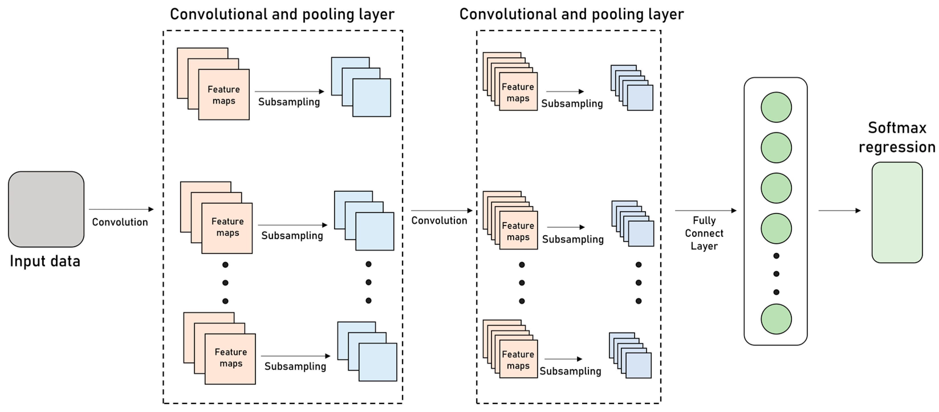
A typical neural network consists of the following elements: convolutional layers, pooling layers, a fully connected layer with a standard classification model, and an activation function at the end to conclude the classification. An example of this type of network can be seen in Figure 2. This architecture is effective in image classification, object recognition, and tasks related to computer vision ([9,13]).
In the input layer, data to be evaluated by the neural network are inserted. These data can be either 2D images or 1D vectors. Since the CNN method is considered supervised, it requires that the data be categorized with their respective classes so that the network can calculate the error.
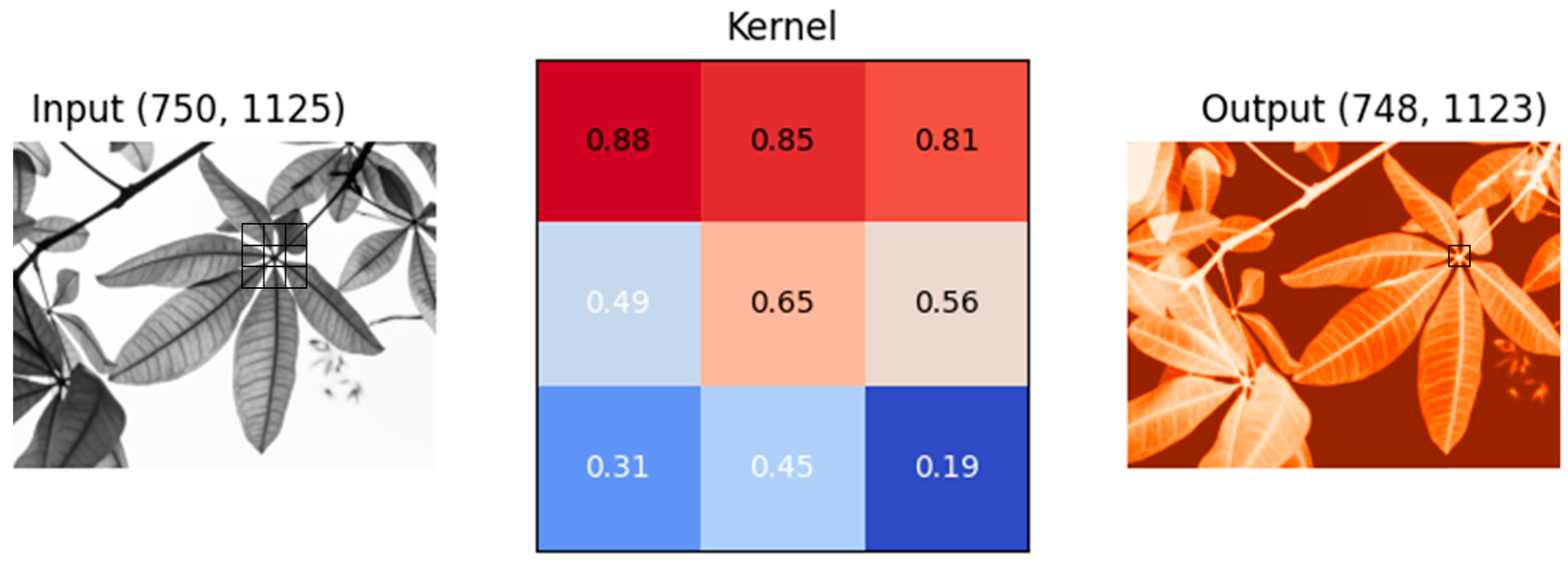
The convolutional layers are the essential components of CNNs. They contain kernels or filters, which are matrices containing representations of specific features to be extracted. The result of applying these kernels is feature maps, which have dimensions smaller than that of the input layer.
The operation of kernels involves traversing the input matrix and extracting the most relevant features from the image. In other words, these elements are square matrices representing “weights” that enhance what is most important (such as edges, contrasting regions, and defined shapes) ([13]). An example of how kernels function can be seen in Figure 3.
The features that the kernel emphasize can be determined manually, but modern libraries and programmatic methods allow for automatic feature extraction. However, other hyperparameters, such as the size of the square matrix, padding, and stride, must be optimized for each problem ([19]).
In simpler applications, the kernel size is typically between 3 × 3 and 6 × 6. Generally, a larger kernel extracts less information, leading to a faster reduction in dimensionality in the layer but with a decrease in network accuracy. On the other hand, a smaller kernel can extract more features, resulting in a more accurate network but requiring more computational power. It is worth noting that a side effect of a smaller kernel can be the capture of undesired or unexpected features that negatively impact the network’s accuracy.
Padding allows for the preservation of data at the edges of activation maps, creating deeper networks but demanding more computational power. Stride determines how much the kernel moves at each step. Typically, the kernel moves one item at a time, and its impact follows a similar pattern to the kernel size, potentially leading to the issue of capturing unwanted features ([2,20]).
At the end of each convolutional layer, each generated feature map undergoes a non-linear activation function, enabling complex representations that would be impossible if the model were composed solely of linear functions, essentially summarized in a linear model ([21]). The more hidden (intermediate) layers with non-linear functions, the higher the abstractions in the network. There are various activation functions, such as the Rectified Linear Unit (ReLU), LeakyReLU, and softmax.
The mathematical representation of the convolution layer can be seen in Equation (11):
x j l = f i x i l 1 k i j l + b j l
where x j l is the j-th feature map produced by the l-th layer, x i l 1 is the ith feature map, k i j l is the j-th kernel that is linked to the ith feature map, b j l is the bias associated with the j-th kernel, * represents the convolution operator in two dimensions (since the problem deals with image), and f is the activation function.
A commonly used activation function in intermediate layers is ReLU due to its practical computational efficiency in classification problems ([22]). Its function and derivative are calculated with Equations (12) and (13):
f x = x + = max 0 ,   x = x   i f   x > 0 ,   0   o t h e r w i s e ,
f x = 1   i f   x > 0 0   i f   x < 0
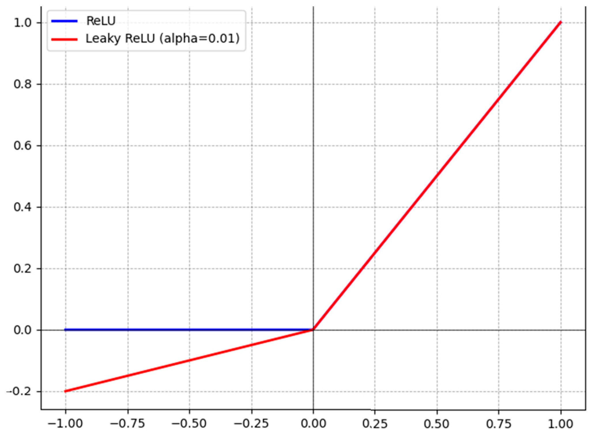
It is worth noting that its zeroes out negative values and returns the same value for positive values. Despite being widely used, a significant drawback of this function is the issue of the “dead neuron”. In this situation, during training, the neuron’s values become zero and become insensitive to further training, losing the ability to learn.
This situation is part of the problem of gradient vanishing in networks with gradient-based learning methods like backpropagation. It occurs when the gradient becomes so small that the ability to change the weights in the neuron is lost, effectively deactivating it ([22]).
Considering the issue with the ReLU function, the LeakyReLU variant has been introduced. In this function, the negative part does not become zero but instead becomes a linear function with a small positive slope. This reduces the chance of returning zero values and mitigates the problem of the “dead neuron”. It is calculated with Equation (14) and can be visualized in Figure 4 alongside the ReLU function.
f x = x   i f   x > 0 ,   α x   i f   x 0
The softmax function is widely used in the output layer of neural networks. It is calculated with Equation (15):
S o f t m a x x i = S ( x i ) = exp x i j e x p ( x j )
where i is the index of the output neuron, and j represents the indexes of all neurons in a level. This function guarantees that, at the network output, the sum of the output values is 1. Thus, this function is used as a probability indicator for each item in problems with more than two possible outputs. For example, in a problem with four possible outputs, A, B, C, and D, a possible case is S x A = 0.20 ,   S x B = 0.10 ,   S x C = 0.63   e   S x D = 0.07 . Adding the probabilities, we have a total of 1.0.
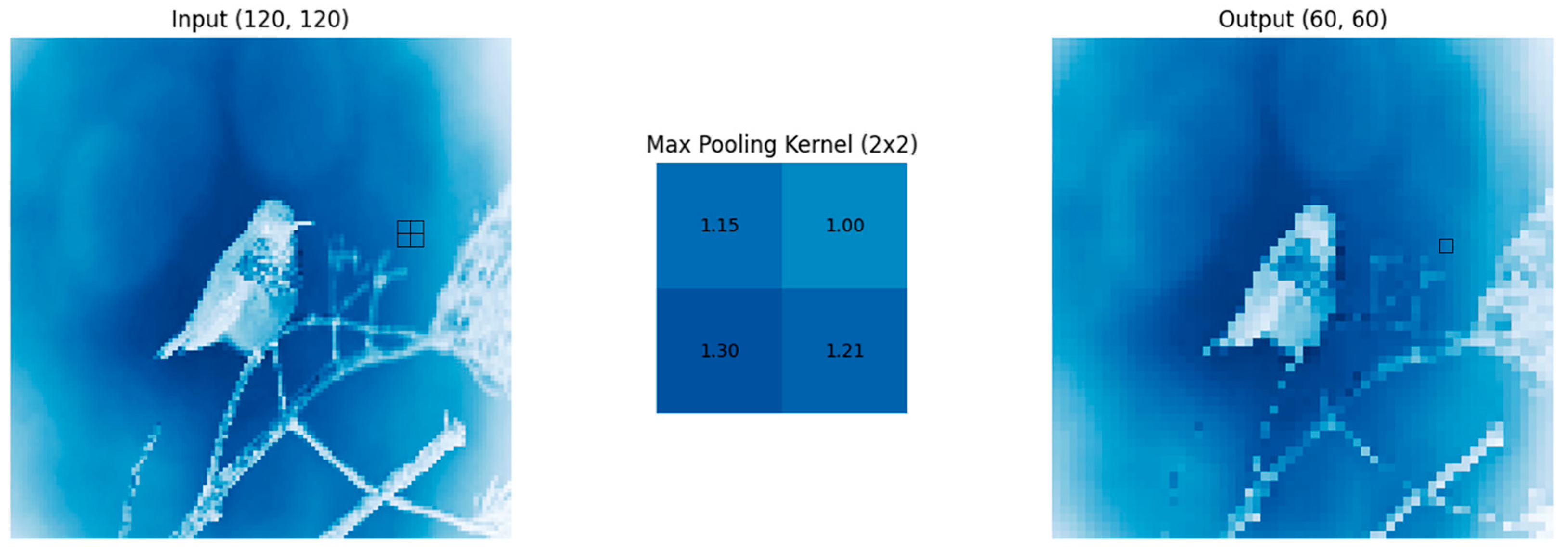
Following the convolutional layers, pooling layers reduce dimensionality while preserving essential features and making the network invariant to small transformations or distortions, thereby improving the computational efficiency of the model. Similar to the convolutional layer, the pooling layer has kernels that, through some defined strategy, perform this operation on the input data. The most common pooling strategies are max pooling (selects the maximum value from the kernel), average-pooling (calculates the average value of the kernel), and stochastic pooling ([8]).
The structure of a layer with max pooling can be seen in Figure 5. In this example, the highest value in the kernel for the analyzed point is 1.3, so that value is chosen. It is noteworthy that, despite reducing both X and Y by half, the output still manages to preserve the main characteristics of the original image.
After passing through one or more sets of convolutional and pooling layers, a CNN is finalized with a fully connected (FC) network and a classification function. The FC network connects each neuron in one layer to every neuron in the adjacent layer. The primary function of the FC layer is to convert the 2D feature maps into a 1D feature vector and synthesize the local information in the simple features extracted by the convolutional and pooling layers. Finally, the processed feature vector is fed into the softmax layer, calculated with Equation (15), to produce the probability score for each class, and the class with the highest score will be the classification result. In Figure 6, the FC layer and the output layer can be observed on the right.
While STFT, CWT, and CNN are established methods in fault diagnosis, the innovative aspect of this study lies in the synergistic integration of these techniques, tailored specifically for the complexities of diesel engine fault detection. By combining the time-frequency resolution of STFT and CWT with the pattern recognition capabilities of CNN, this research not only enhances the fault detection process but also addresses the challenges of real-time application in industrial environments. The methodological advancements include optimizing the CNN architecture to work effectively with the signal pre-processing outputs, leading to significant improvements in fault classification accuracy, even under high noise conditions.

3. Methodology

3.1. Problem Modeling

In this study, torsional vibration data from a diesel engine are utilized. These data were obtained through computational simulations of faults in a 6-cylinder, in-line diesel engine and subsequently validated with the manufacturer. In [17], the authors conducted these simulations, and the resulting generated data were made available through the 3500-DEFault dataset, publicly accessible among the datasets on the Mendeley platform ([23]), serving as the data source for this research.
This type of vibration can be characterized as a fluctuation in the crankshaft’s rotational speed caused by the periodic nature of combustion and the inertial movement of the engine’s moving parts. Such vibration is primarily detectable in the engine’s crankshaft ([24,25]). Various measurement methods can be applied, such as using two linear accelerometers positioned diametrically opposite on the shaft’s surface (eliminating translational movement), angular accelerometers (positioned on the cross-sectional face of the shaft), strain gauges, magnetic sensors, or laser interferometers (more expensive and used in a controlled environment) ([26]).
The engine was evaluated under normal operating conditions and three other abnormal operating conditions (faults), which are described below:
  • Normal condition;
  • Reduced air intake manifold pressure;
  • Reduced compression pressure in each of the cylinders;
  • Reduced amount of fuel injected into the cylinders.
The data correspond to the supercharged marine diesel engine Acteon 6.12TCE manufactured by MWM Diesel Motors ([27]). Table 1 presents the physical and operational characteristics of the engine used as the basis for generating simulated fault data.
To conduct the simulation, Ref. [17] considered the following models:
  • Zero-dimensional thermodynamic model (0D).
  • Concentrated mass model for torsional vibration in the crankshaft.
  • Fault simulation model.
The thermodynamic model was validated by comparing the pressure curves within the cylinder, while the computational model of torsional vibration used the nominal engine output torque curve, both provided by the aforementioned engine manufacturer.
The adopted mathematical thermodynamic model is the zero-dimensional or single-zone thermodynamic model based on the first law of thermodynamics and the equation of state. Its purpose is to obtain pressure data of the gasses inside the cylinder as a function of the crankshaft angle. It assumes that the gas mixture inside the cylinder during the intake and exhaust processes occurs at constant pressure, so the compression moment can be considered as a polytropic process, as expressed in Equation (16). It is noted that these values depend on the angular position of the crankshaft, denoted by θ ([27]).
d P d θ = n P V d V d θ
The mass flow of air during the intake and exhaust processes is steady, and the control volume considered in this zero-dimensional model is illustrated in Figure 7, represented by the engine cylinder.
From the first law of thermodynamics and considering losses due to convection and radiation, one can derive Equation (17), which represents the rate of temperature change in the gas mixture in the cylinder:
d T d θ = δ Q t d θ δ Q w d θ P d V d θ 1 m c v
where δ Q t d θ is heat supplied to the system due to fuel burning, δ Q w d θ is the heat loss to the cylinder walls, and δ Q w d θ is the volume of the combustion chamber. All these items are dependent on the angular position θ of the crankshaft. P, m, and c v represent, respectively, the instantaneous pressure of the gasses, the mass of the gas mixture, and the specific heat at constant volume of the mixture.
As a zero-dimensional model was considered, it can be stated that the gas inside the cylinder behaves ideally. Therefore, the pressure variation depending on the crankshaft position d P d θ can be calculated with Equation (18):
d P d θ = m R d T d θ P d V d θ 1 V  
where P is the internal pressure in the cylinder (in pascals), m is the mass in kilograms of air in the cylinder, R is the universal gas constant, V is the volume of the cylinder at position θ, and T is the temperature of the mixture inside the cylinder ([17]).
In addition to the thermodynamic model, the concentrated mass model must be included to represent the dynamics of the moving parts of the engine. This model represents the dynamics of the crankshaft, considering two torsional dampers, the crankshaft pulley, a set of gears for power transmission to other parts of the engine, the six cylinders, and the flywheel. Considering Newton’s second law, Equation (19) is obtained:
J θ ¨ ( t ) + C θ ˙ ( t ) + K θ ( t ) = { M ( t ) }  
where [J] is the torsional matrix, [C] is the damping matrix, and [K] is the system stiffness matrix. θ ¨ ( t ) , θ ˙ ( t ) , and θ ( t ) are, respectively, the angular acceleration, angular velocity, and angular position of the crankshaft in vector form. Finally, {M(t)} is the moment vector about the axis.
From this theoretical model, it is possible to define a torsional vibration model. In practice, this is intrinsic to the operation of a combustion engine, given that the crankshaft experiences the application of inertial torques due to the reciprocating motion of moving components (piston, connecting rod, rings, etc.) and combustion torques due to fuel burning in the chamber. In both cases, the torque application is not constant but oscillatory ([17,28]). In other words, they depend on the angular position of the crankshaft. The load due to inertia is calculated with Equation (20), and the load due to combustion is calculated with Equation (21):
F r = m r r Ω 2 ( cos θ + l cos 2 θ l 3 4 cos 4 θ + 9 l 5 128 cos 6 θ )
F c = P π D 2 4
The moment is then calculated with Equation (22):
M = r F r + F c sin θ + cos θ tan γ
The variable m r is the alternating mass, r is the crankshaft radius, Ω is the crankshaft rotation speed in rad/s, and l is the ratio between the crankshaft radius and the connecting rod length. The gamma variable is dependent on θ and is calculated as follows:
γ = l sin θ 1 l 2 4 + l 2 4 cos 2 θ
The simulation results are compared with experimental pressure and torque curves provided by the manufacturer. In Figure 8, simulated pressure curves inside the cylinder are observed compared with actual curves for 1000, 1900, 2300 RPM, and 2500 RPM. According to [17,27], the smallest errors for maximum pressure and mean pressure are 0% and 5%, respectively.
The utilized database consists of a total of 3500 different signals related to the torsional vibration of the crankshaft. These data were constructed using numerical simulation based on the detailed engine model described earlier and were generated considering the engine rotating at 2500 RPM. This RPM was chosen because, during the validation stage of the thermodynamic models, it demonstrated the lowest combined error in the mean and maximum pressure of the combustion cycle among all observed rotations. The sampling frequency of the data is 15 kHz ([17]).
The database provided by [23] and used in this study contains data with various levels of added noise, including 0 dB (no noise), 15 dB, 30 dB, and 60 dB. However, as this study evaluates a new method, we chose to work with data at 0 dB. Subsequently, noise values at other intensities will be manually added to thoroughly evaluate the model’s performance beyond the originally published values.
Among the various possible faults that can occur in a diesel engine, thermodynamic faults were chosen for this study. The signals are divided into the following:
  • 250 signals for the normal condition;
  • 250 signals for the reduced air intake pressure condition, ∆Pi, caused, for example, by turbocharger malfunction or corrosion of the intake valve;
  • 1500 signals for the reduced compression ratio condition, ∆r, in the cylinders, due to piston corrosion or clearance;
  • 1500 signals for the reduced fuel quantity condition, ∆m, injected into the cylinders.
Each signal represents a capture of torsional vibration for a certain period. The second case is a general problem that affects all cylinders. The third and fourth cases are local faults for each cylinder. Thus, the fault vector can be defined by Equation (24):
f = P i ,   m c j ,   r j ,   j = 1 ,   2 ,   3 ,   4 ,   5 ,   6
where j is the cylinder number. Each item in this vector is a failure given as a percentage of the value under normal operating conditions.
Equally important, [17] develop the data and application of severity as described below. As it is simulated data, it applies a small percentage of severity in the normal case. This severity, contained in a range of 0 to 0.1%, was distributed with a uniform probability among the physical variables used in the simulation. With this, we want to simulate real operating conditions in which the engine operates with small variations around optimal operation.
In the second condition above, pressure severity values were added to the manifold in increments of 0.2%, that is, P r 1.0 ,   1.2 ,   1.4 ,   ,   49.8 ,   50 in percentage, totaling 250 signals, where P r represents the pressure variation applied to the normal operating pressure in the manifold.
In the last two cases, both with 1500 points, the severities were applied to each cylinder. Thus, in cylinder i, i { 1 ,   2 ,   3 ,   4 ,   5 ,   6 } , and there are several scenarios with severities r i 1.0 ,   1.2 ,   1.4 ,   ,   49.8 ,   50 and m c i 1.0 ,   1.2 ,   1.4 ,   ,   49.8 ,   50 , where r i is the increment applied to the compression ratio in normal operation r in cylinder i, and m c i is the increment in the mass flow of fuel in the mass flow in normal operation m c in cylinder i. Therefore, as there are 250 signals in each interval, where each one is applied to each of the six cylinders, there are a total of 1500 signals for each of severities 3 and 4.

3.2. Numerical Modeling

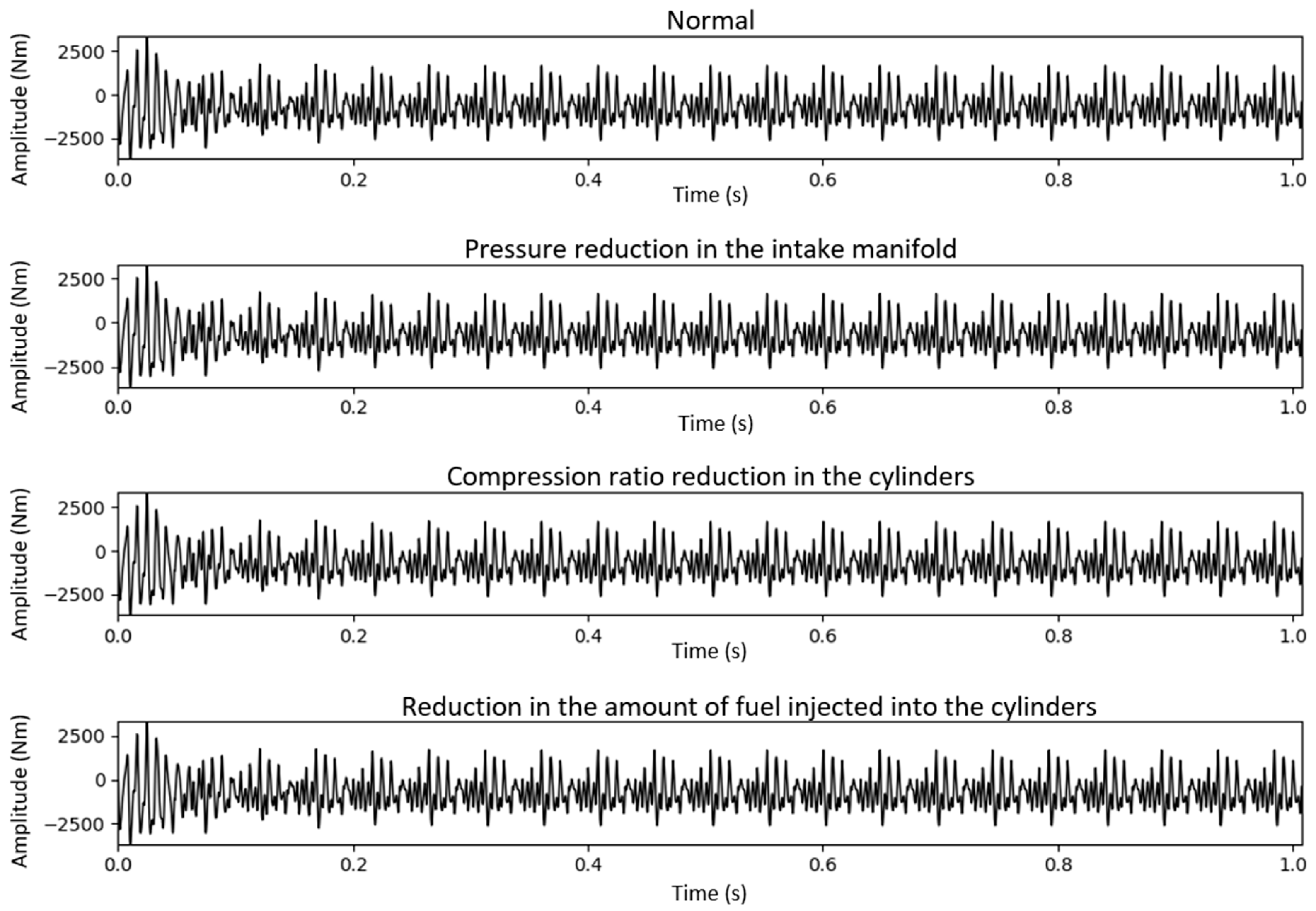
The torsional vibration data obtained from the computational simulation process explained in Section 3.1 are displayed in Figure 9, where the signal corresponding to the first point of each operational condition can be observed. It is evident that based solely on the time-domain vibration signals, it is not possible to distinguish and classify the signals for each type of operational condition. Therefore, the use of signal-processing techniques is necessary to extract more information from the signal.
Thus, these signals are pre-processed using short-time Fourier transform (STFT) and continuous wavelet transform (CWT), giving rise to spectrograms and scalograms, respectively. For each of the 3500 data points, both transforms are applied, resulting in a total of 3500 spectrograms and 3500 scalograms.
To represent the short-time Fourier transform (STFT) and generate spectrograms, the ‘spectrogram’ function from the SciPy library in Python was used. The Blackman window function ([29]) was chosen as the parameter for the window function w(τ), with a length of 256 segments. It was observed that the frequency values were low, so the graphs were limited with an upper limit of 1000 Hz.
For generating scalograms to represent the continuous wavelet transform (CWT) output, the ‘CWT’ function from the ObsPy library was used. By default, the mother wavelet is represented by the Morlet function ([30]), with an initial maximum frequency of 2000 Hz and an initial minimum frequency of 1 Hz. These frequencies were chosen through experimentation and by observing the occurrence of low frequencies in the STFT. An upper margin was left for data analysis; however, it was noticed that the values, in this case, also remained below 1000 Hz. Therefore, the same upper limit as in the STFT was subsequently adopted. This observation is valid given that the rotation at which the data were generated is 2500 RPM or 46.67 Hz.
An example spectrogram and scalogram for each operating condition is presented in Figure 10 and Figure 11, respectively. Frequency is distributed on the y axis and time on the x axis. The z axis represents the signal amplitude.
The differences between the conditions are practically imperceptible to the naked eye, demonstrating that even with signal analysis training, fault detection aided by neural networks proves to be an excellent alternative in this situation.
To assess the robustness of the developed model and simulate data measured in a real experimental condition, white noise was applied to the Gaussian-type data (White Gaussian Noise or WGN). It is generated and added to each of the analyzed vibration signals. In addition to 0 dB, five different noise levels were applied to the data, obtained by the inverse of the signal-to-noise ratio (SNR) ([31]), namely: 10%, 20%, 40%, 60%, and 80%. The equation for SNR is calculated with Equation (25) in percentage and by Equation (26) in decibels.
S N R = S i g n a l   p o w e r N o i s e   p o w e r = S R = 100 %   n o i s e
S N R d B = S d B R d B
You must convert the value from powers to decibels. Therefore, Equation (27) applies, where j indicates whether it is an original signal or noise.
S N R j , d B = 10 log 10 S N R j
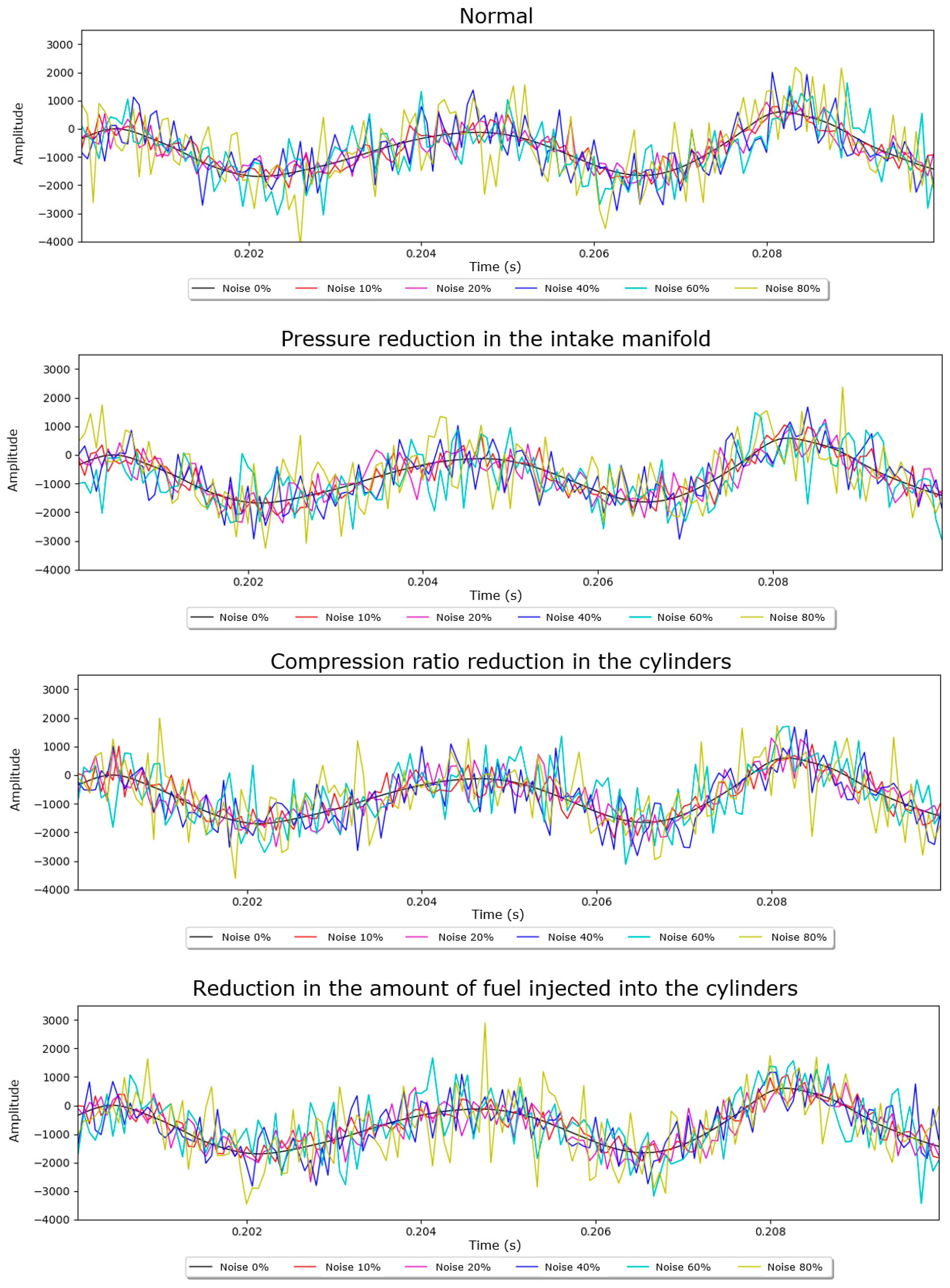
With the signal in watts, the mean is extracted and converted to decibels using Equation (27). Finally, to generate random noise, a random function with a normal distribution, having a mean of zero and variance equal to RdB, is employed. The randomly generated values are then added to the original signal, resulting in the noisy signal. In Figure 12, samples of the data with noise can be observed.
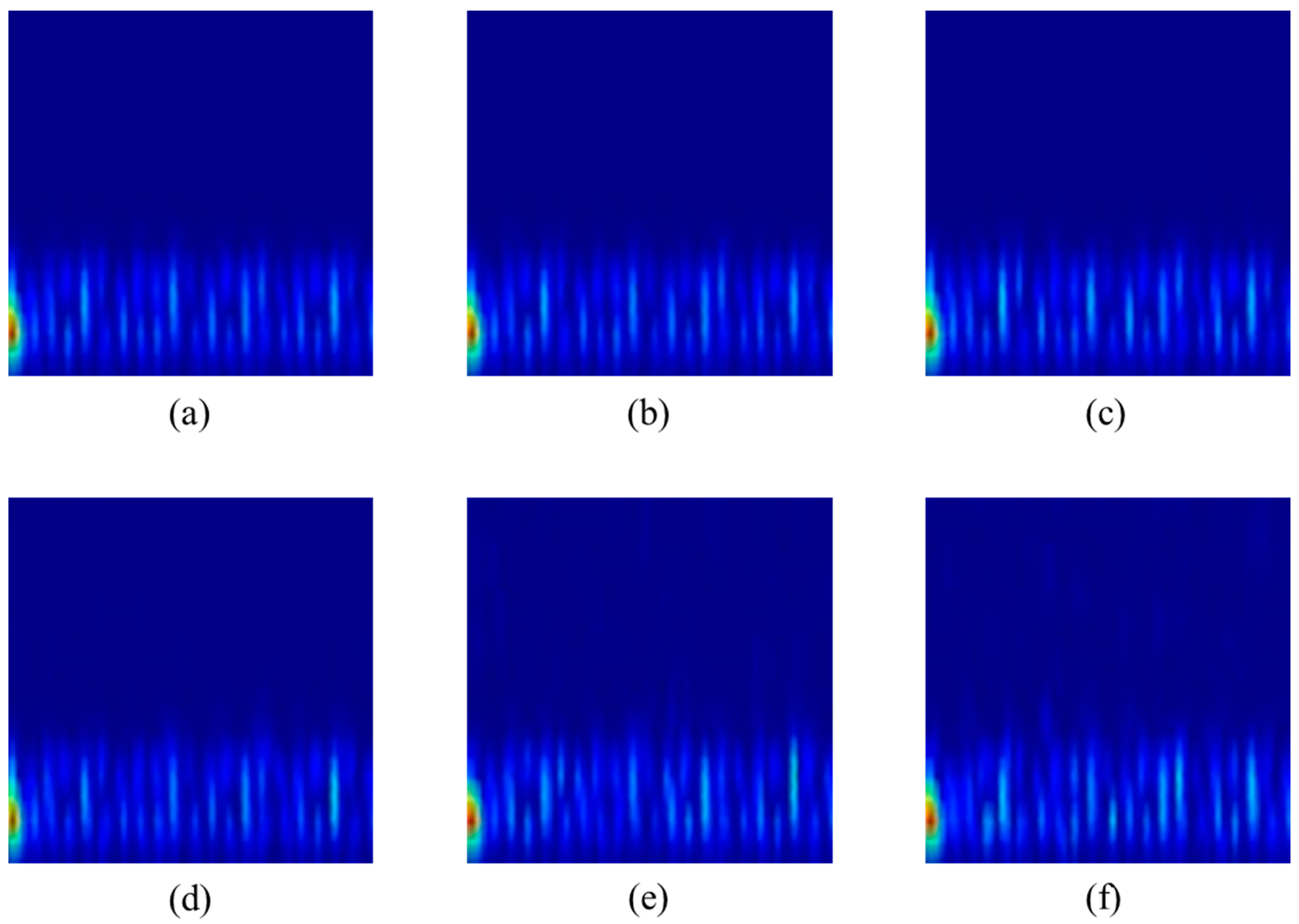
In the same way as the noise-free signals (0 dB), 3500 images were generated for each noise level mentioned above. In Figure 13 and Figure 14, there are examples for the normal case.
The neural network scripts and optimization processes were executed on a computer with the following configuration: AMD Ryzen 5 5600 H processor, 16 GB of RAM, and an NVIDIA GeForce RTX 3060 graphics card. It is important to note that the processing was mainly carried out by the processor, although there are other software acceleration methods that utilize the graphics card, making the process much faster.

3.3. Convolutinal Neural Network Architecture

Among the 3500 images of spectrograms (STFT) and scalograms (CWT), 75% were used for training, and the remaining 25% were used for testing. The data were loaded and automatically split between these groups using the ‘train_test_split’ function from the scikit-learn library. The convolutional neural network was created using the Keras library. Three convolutional layers were used, each with 5 × 5 kernels and a stride of 2 × 2. A LeakyReLU activation function with an alpha of 0.3 and an L2 filter regularizer were assigned to each convolutional layer. This regularizer helps prevent overfitting, ensuring the network has generalized capacity to identify new examples beyond those used for training. Following each convolutional layer, a max-pooling layer with a 2 × 2 filter and a dropout layer were applied. Dropout temporarily turns off the connections both before and after a neuron, essentially creating a new network. This neuron selection is determined by the dropout probability (p), and it also helps prevent overfitting ([8]). The final fully connected (FC) layer adopted the softmax activation function, and the ADAM algorithm was used as the optimizer.
To configure the neural network training, several parameters needed to be defined, including the learning rate, batch size, and number of epochs. The learning rate significantly influences the determination of weights in the neural network. Batch size allows the separation of training data into small groups to avoid computational overload. The number of epochs controls how many times the algorithm will run during training with each data block. These parameters were chosen through trial and error ([13]).
Initially, the batch size and epochs were kept constant at 64 and 500, respectively. The learning rate was varied using values in {0.0001, 0.0005, 0.001, 0.005, 0.01, 0.05}. The highest accuracy was achieved with 0.001. With this new value, the batch size was varied from 8 to 64, with intermediate multiples of 8, achieving the best accuracy with a value of 16. Finally, the number of epochs was varied in the same way, ranging from 0 to 500, with a step of 100. Here, not many changes in accuracy were observed, so 500 epochs were set. This configuration was used in all procedures.
For hyperparameter tuning, the ‘keras_tuner’ library was used, allowing the insertion of intervals or lists of possibilities for numerical, non-numerical, and binary fields contained in the network construction. For example, for the L2 regularizer value fields, a test range from 10−4 to 0.1 was adopted. This allowed the evaluation of various points and combinations of hyperparameters during the training process. Other fields tested included dropout values ranging from 0.015 to 0.15 and the number of dense units in the last FC layer, varying integer values between 16 and 512 with a step of 16 units. The hyperparameter optimization process is performed automatically using the Bayesian optimization algorithm with the stipulated goal of achieving the highest accuracy.
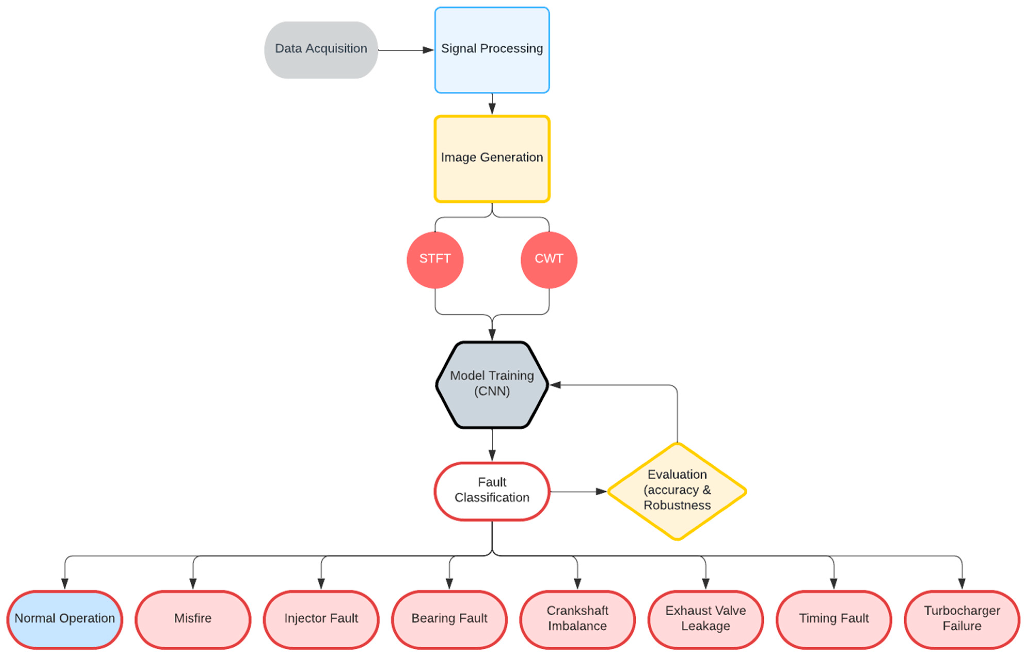
To provide a clear overview of the proposed methodology, a block diagram along with the corresponding algorithm is presented in Figure 15. This diagram outlines the key steps involved in the fault detection process, including data acquisition, signal processing, image generation, model training, fault classification, and evaluation. The algorithm accompanying the block diagram details the sequential procedures followed in this study, highlighting the integration of short-time Fourier transform (STFT) and continuous wavelet transform (CWT) techniques with convolutional neural networks (CNNs) to accurately classify various engine fault types.

4. Results and Discussion

4.1. CNN–STFT Network

The script for generating images with signals transformed by STFT had a relatively fast execution time, generating the 3500 images in about 10 min. The training process was also relatively fast, taking an average of 4 to 5 min.
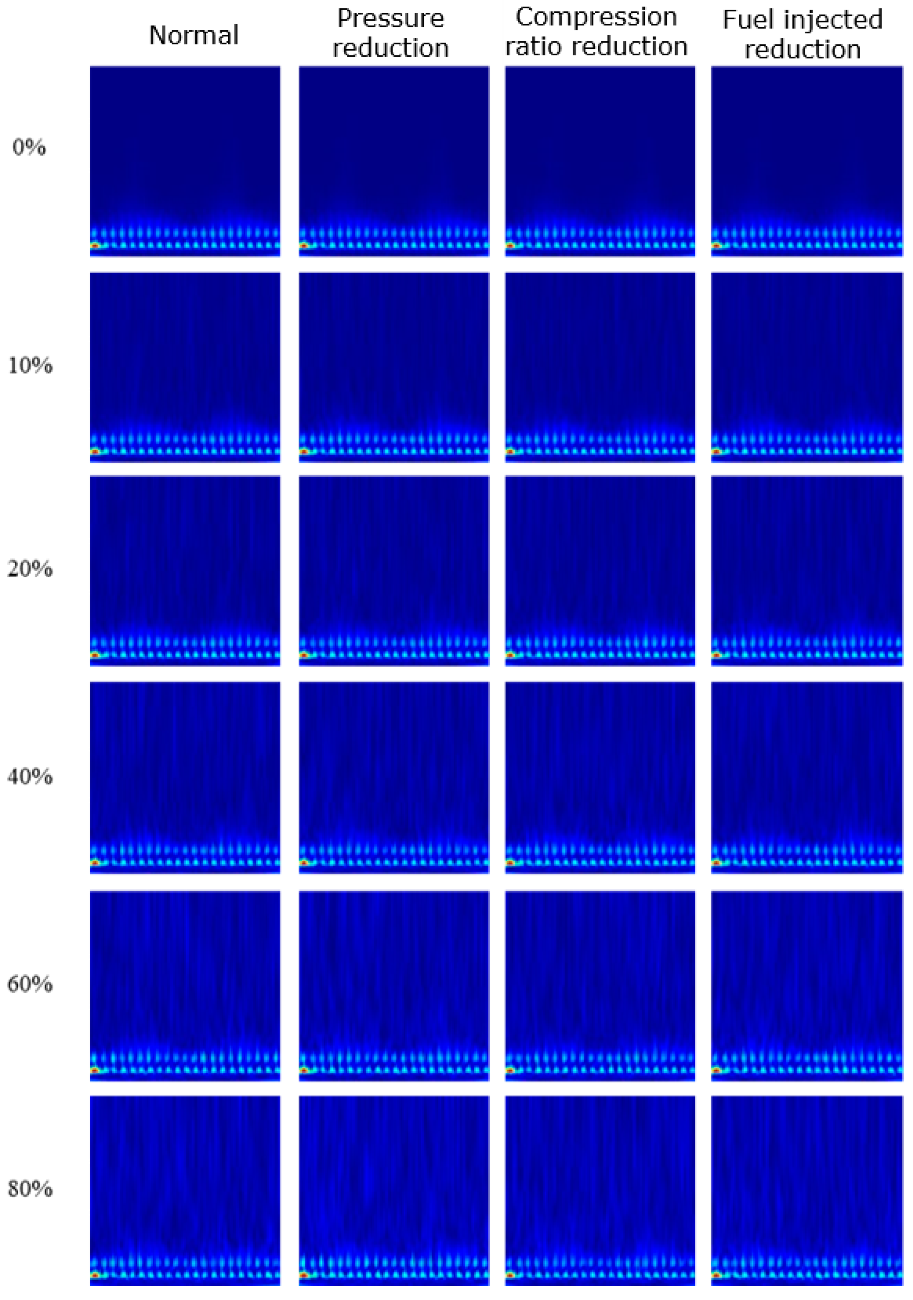
To evaluate the results obtained from the described methodology, Figure 16 presents the vibration signals transformed by STFT for each type of condition studied and at each noise level. It is noticeable in this figure that this transform is not very sensitive to noise, with some differences only becoming apparent after the 40% noise level. Additionally, there is little definition in the spectrograms along the frequency axis, even when varying the search window size. This is a characteristic of this transform, which needs to make a trade-off in resolution between time and frequency, sometimes not defining both well ([3]).
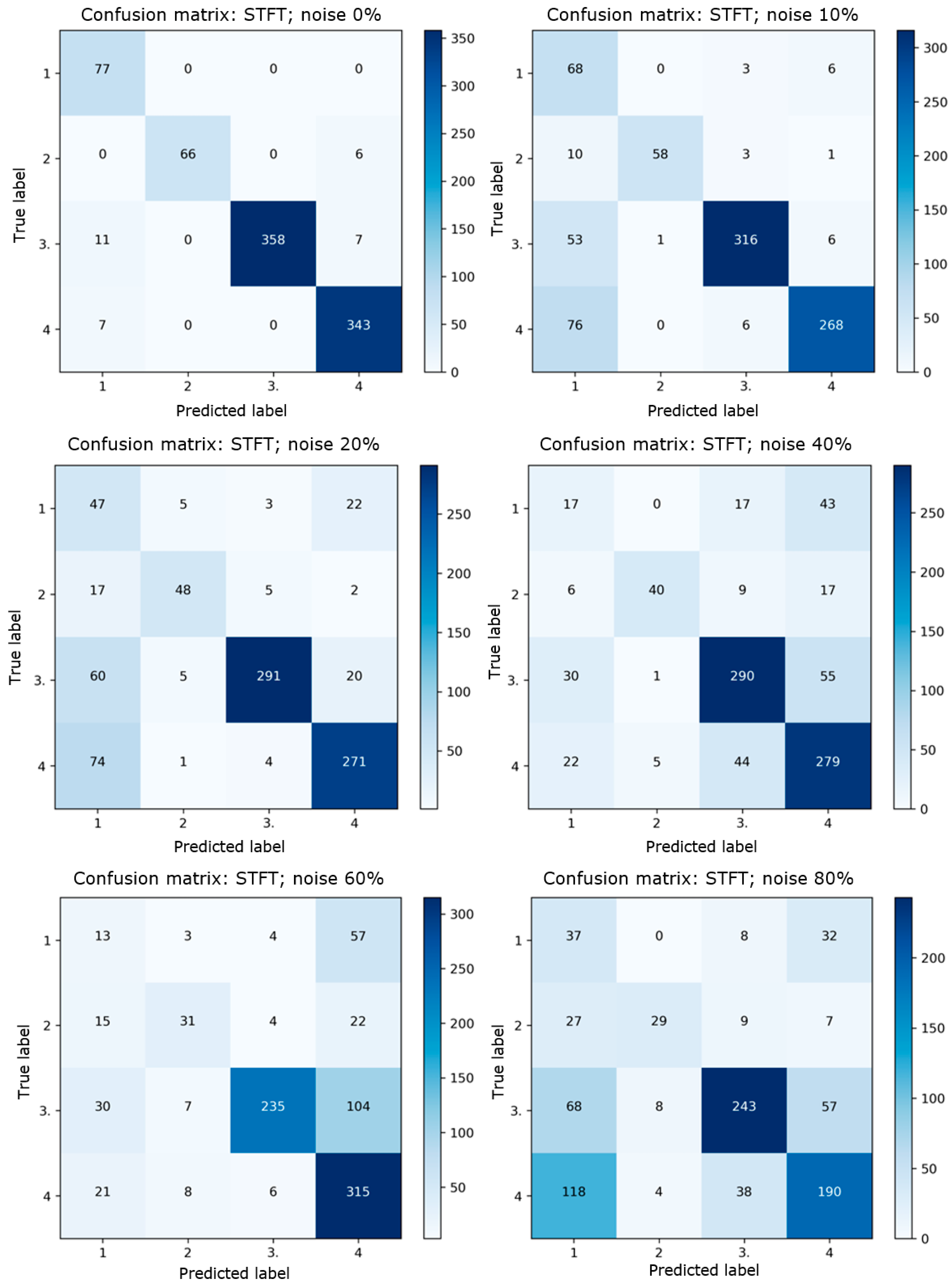
In Figure 17, the confusion matrix set is highlighted for each noise level. Here, 25% of the data were applied to evaluate the network, totaling 875 figures (approximately divided according to the proportion of the number of images between each class). Case 1 represents normal conditions, Case 2 is reduced pressure, Case 3 is reduced compression ratio, and Case 4 is reduced fuel. The main diagonal represents correct predictions, while other elements indicate incorrect predictions. A good overall performance is noticeable, especially up to 20%, achieving an accuracy of 96.5% for noise-free signals, 81.1% for 10% noise, and 75.1% for 20% noise. However, it is worth noting a specific difficulty of the network in classifying images between reduced fuel and normal, with many false predictions between these two classes. With high noise, these difficulties became much more evident, with accuracies lower than 72%, reaching 57% with 80% noise.

4.2. CNN–CWT Network

Contrary to the images generated by STFT, using the CWT with the signals resulted in a much longer runtime, taking several hours to generate the 3500 images. The training process was also more time-consuming, lasting approximately 30 min.
To evaluate the results obtained from the described methodology, Figure 18 presents the vibration signals transformed by CWT for each type of condition studied and at each noise level. In this case, the impact of noise is already noticeable at 10%, becoming more intense at higher levels. This aligns with the method’s sensitivity to frequency variations over time.
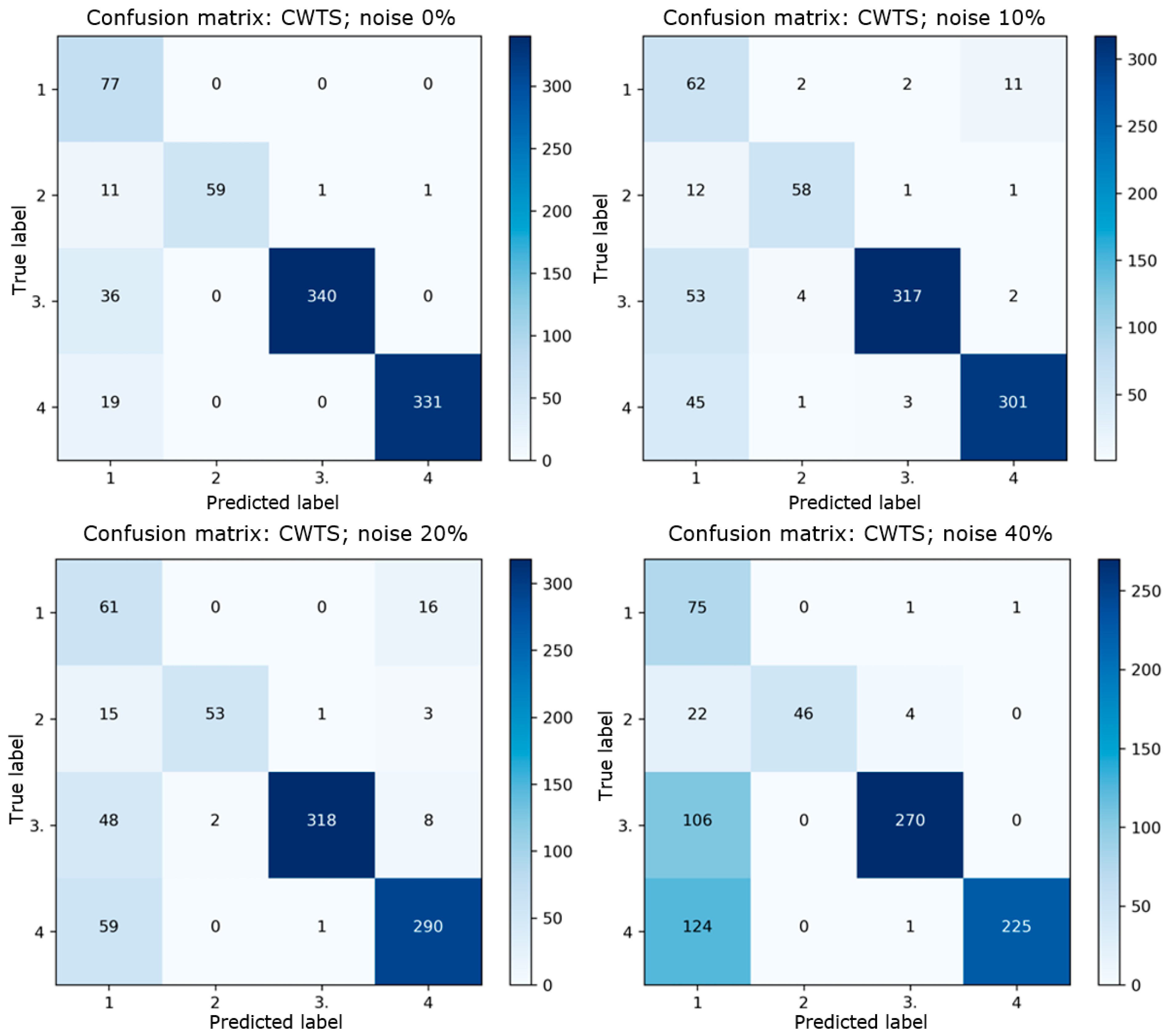
In Figure 19, similar to the previous presentation, the confusion matrix set is highlighted for each noise level. Once again, Case 1 represents normal conditions, Case 2 is reduced pressure, Case 3 is reduced compression ratio, and Case 4 is reduced fuel. The main diagonal represents correct predictions, while other elements indicate incorrect predictions. The evaluation was applied to the same number of test images. Overall, a better performance is evident compared to the application of STFT in all cases. However, there is again a certain difficulty in separating the normal and reduced fuel classes.

4.3. Results Comparison

In general, by observing Figure 16 and Figure 17, it is apparent that the STFT has shown low sensitivity to noise, with traces becoming noticeable only from 60% noise level. In contrast, with the CWT, noise is distinctly present as early as 10%, and the signal becomes significantly noisy from 40% onwards. This can be explained by the fact that the CWT adapts better to signals undergoing frequency changes over time, and in this case, the signal remains in a steady state for most of the graph. However, it is worth noting that in the CWT, the signal performs better at the beginning of the time on the left side of the graph, where there is a peak in signal amplitude. This peak, caused by the engine start, creates a brief transient effect, making the signal less sensitive to noise.
From Figure 20, Figure 21, Figure 22 and Figure 23, the output of the initial convolutional layers, pooling, and dropout layers for both the STFT and CWT networks can be observed for each case among the classes with 20% noise (as an example). The figures depict the filtering of characteristics and the selection of the most relevant ones, highlighted by more intense colors. Additionally, the output of the max-pooling layer, which selects the most intense features, is noteworthy.
In addition to comparing the performance of the proposed method with different signal-processing techniques (STFT and CWT), we conducted a comparative analysis with other well-established fault classification methods based on vibration signal analysis. Specifically, we compared our approach with methods such as support vector machines (SVMs), random forest (RF), and traditional artificial neural networks (ANNs) using the same dataset.
In Table 2, detailed accuracy values for each transform are provided, categorized by noise level. It is evident that, in both cases, using each transform yielded approximately comparable values up to 40% noise, followed by a sharp decline when using STFT and a consistent performance when using CWT.
As previously mentioned, the use of the wavelet transform has allowed for higher levels of accuracy when compared to the STFT; however, it requires significantly more execution time. Therefore, the choice between them may depend on the practical application. For instance, STFT can be applied in embedded systems for real-time analysis of a diesel engine, while CWT may be utilized for periodic equipment assessments using more powerful computers.
This comparative analysis underscores the effectiveness of our method not only in ideal conditions but also in more challenging, real-world scenarios where noise is a significant factor. The results confirm that the combination of CNN with advanced signal-processing techniques provides a more reliable and accurate solution for fault classification in diesel engines compared to conventional methods.
It is worth noting, however, that there is a fast version of the wavelet transform, which can be explored as an alternative to CWT, potentially addressing the computational cost issue associated with this transform. Furthermore, another viable approach is to combine multiple transforms to blend the best characteristics of both methods.

5. Conclusions

From the obtained results, it can be said that the proposed methodology for identification and classification of faults in diesel engines demonstrates overall good performance, achieving accuracy values that exceed 70% for average noise levels. The continuous wavelet transform (CWT) stood out in robustness, maintaining good accuracies even for high noise levels, demonstrating that the network was better adapted for use with this transform. However, it is worth noting that, even with the use of an automatic tuning function for some hyperparameters, it may be necessary to expand the parameters evaluated automatically to generate networks better suited for each situation.
Another possible reason for the better performance of using the wavelet transform may be explained by the fact that there are more variations in the signal’s frequency, especially at the beginning, representing the motor’s startup in practice. These frequency variations over time are better captured by this transform, as described in the literature and demonstrated in practice.
On the other hand, it is crucial to emphasize that the use of the continuous wavelet transform (CWT) requires much more extensive computational power, which also reflects in a much longer processing time for signal processing. This can affect its practical use in a continuous learning situation (where the process of capturing, processing, and training the network occurs continuously throughout the motor’s operation), as it is often not possible to have access to a supercomputer in the field, making its use completely unfeasible. Thus, in these cases, the short-time Fourier transform (STFT) has a significant advantage, as it can be used on simpler and more cost-effective devices. Therefore, if there is access to good computational power, the CWT may be the better option; in the opposite case, if access is more restricted, the STFT can still be used with a good level of reliability.
Hence, it is valid to say that there is potential to apply the proposed identification method in this work to real-world problems, as there are various ways to capture the torsional vibration of an engine, including several low-cost options (such as the use of strain gauges). Moreover, with the same setup, it is possible to expand the number of studied fault classes since torsional vibration can capture other problems, especially structural ones, as observed in this work and in other sources in the literature with proposals in the same field.
Future work should consider the application of experimental torsional vibration data to further validate the fault-detection methods and neural network models developed in this study. Additionally, exploring various neural network configurations and parameters to optimize real-time analysis of engine conditions presents a promising avenue for improvement. Investigating the combined use of different signal transforms within the network and conducting comprehensive hyperparameter tuning will be essential to refining the model’s accuracy and adaptability. Expanding the scope of the study to include a wider variety of combustion engine faults will provide a more robust assessment of the proposed methodology. Furthermore, evaluating the effectiveness of the neural network and signal-processing techniques with other types of signals, such as thermal and acoustic data, could offer additional insights and enhance the model’s applicability across different diagnostic contexts.

Author Contributions

Conceptualization, G.F.G.; methodology, G.H.F.M., R.F.R.J. and G.F.G.; software, G.H.F.M., R.F.R.J. and G.F.G.; validation, G.H.F.M., R.F.R.J. and G.F.G.; formal analysis, G.H.F.M., R.F.R.J. and G.F.G.; investigation, G.H.F.M., R.F.R.J. and G.F.G.; resources, G.F.G.; data curation, G.H.F.M. and G.F.G.; writing—original draft preparation, G.H.F.M.; writing—review and editing, G.F.G.; visualization, G.H.F.M. and G.F.G.; supervision, G.F.G.; project administration, G.F.G.; funding acquisition, G.F.G. All authors have read and agreed to the published version of the manuscript.

Funding

This research was funded by the National Council for Scientific and Technological Development (CNPq—Grant PQ 307770/2022-2, 405349/2022-0).

Data Availability Statement

All data supporting the reported results can be found in the following repository: https://github.com/gfreire57/ic_engines_CNN_fault_detection (accessed on 26 September 2024). This repository includes all the codes used during the study. No additional datasets were generated.

Acknowledgments

The authors would like to acknowledge the support from the National Council for Scientific and Technological Development, Coordination for the Improvement of Higher Education Personnel (CAPES), and Research Support Foundation of the State of Minas Gerais (FAPEMIG).

Conflicts of Interest

The authors declare no conflicts of interest.

References

  1. Sterkenburg, R. Aircraft Maintenance & Repair, 8th ed.; McGraw-Hill Education: New York, NY, USA, 2019. [Google Scholar]
  2. Kiranyaz, S.; Avci, O.; Abdeljaber, O.; Ince, T.; Gabbouj, M.; Inman, D.J. 1D convolutional neural networks and applications: A survey. Mech. Syst. Signal Process. 2021, 151, 107398. [Google Scholar] [CrossRef]
  3. Al-Badour, F.; Sunar, M.; Cheded, L. Vibration analysis of rotating machinery using time–frequency analysis and wavelet techniques. Mech. Syst. Signal Process. 2011, 25, 2083–2101. [Google Scholar] [CrossRef]
  4. Jing, L.; Zhao, M.; Li, P.; Xu, X. A convolutional neural network based feature learning and fault diagnosis method for the condition monitoring of gearbox. Measurement 2017, 111, 1–10. [Google Scholar] [CrossRef]
  5. Wu, J.-D.; Chen, J.-C. Continuous wavelet transform technique for fault signal diagnosis of internal combustion engines. NDT E Int. 2006, 39, 304–311. [Google Scholar] [CrossRef]
  6. Howlett, R.J.; DeZoysa, M.M.; Walters, S.; Howson, P. Neural Networks Techniques for Monitoring and Control of Internal Combustion Engines. In Proceedings of the International ICSC Symposium on Intelligent Industrial Automation (IIA), Genova, Italy, 1–4 June 1999. [Google Scholar]
  7. Shatnawi, Y.; Al-Khassaweneh, M. Fault Diagnosis in Internal Combustion Engines Using Extension Neural Network. IEEE Trans. Ind. Electron. 2013, 61, 1434–1443. [Google Scholar] [CrossRef]
  8. Zhu, X.; Cai, Z.; Wu, J.; Cheng, Y.; Huang, Q. Convolutional neural network based combustion mode classification for condition monitoring in the supersonic combustor. Acta Astronaut. 2019, 159, 349–357. [Google Scholar] [CrossRef]
  9. Pinedo-Sánchez, L.A.; Mercado-Ravell, D.A.; Carballo-Monsivais, C.A. Vibration analysis in bearings for failure prevention using CNN. J. Braz. Soc. Mech. Sci. Eng. 2020, 42, 628. [Google Scholar] [CrossRef]
  10. Chen, Y.; Rao, M.; Feng, K.; Zuo, M.J. Physics-Informed LSTM hyperparameters selection for gearbox fault detection. Mech. Syst. Signal Process. 2022, 171, 108907. [Google Scholar] [CrossRef]
  11. Firmino, J.L.; Neto, J.M.; Oliveira, A.G.; Silva, J.C.; Mishina, K.V.; Rodrigues, M.C. Misfire detection of an internal combustion engine based on vibration and acoustic analysis. J. Braz. Soc. Mech. Sci. Eng. 2021, 43, 336. [Google Scholar] [CrossRef]
  12. Ni, Q.; Ji, J.; Halkon, B.; Feng, K.; Nandi, A.K. Physics-Informed Residual Network (PIResNet) for rolling element bearing fault diagnostics. Mech. Syst. Signal Process. 2023, 200, 110544. [Google Scholar] [CrossRef]
  13. Ribeiro, R.F., Jr.; Areias, I.A.d.S.; Campos, M.M.; Teixeira, C.E.; da Silva, L.E.B.; Gomes, G.F. Fault Detection and Diagnosis in Electric Motors Using Convolution Neural Network and Short-Time Fourier Transform. J. Vib. Eng. Technol. 2022, 10, 2531–2542. [Google Scholar] [CrossRef]
  14. Uddin, J.; Kang, M.; Nguyen, D.V.; Kim, J.-M. Reliable Fault Classification of Induction Motors Using Texture Feature Extraction and a Multiclass Support Vector Machine. Math. Probl. Eng. 2014, 2014, 814593. [Google Scholar] [CrossRef]
  15. Zabin, M.; Choi, H.-J.; Uddin, J. Hybrid deep transfer learning architecture for industrial fault diagnosis using Hilbert transform and DCNN–LSTM. J. Supercomput. 2022, 79, 5181–5200. [Google Scholar] [CrossRef]
  16. Shahid, S.M.; Ko, S.; Kwon, S. Real-time abnormality detection and classification in diesel engine operations with convolutional neural network. Expert Syst. Appl. 2022, 192, 116233. [Google Scholar] [CrossRef]
  17. Viana, D.P.; de Sá Só Martins, D.H.C.; de Lima, A.A.; Silva, F.; Pinto, M.F.; Gutiérrez, R.H.R.; Monteiro, U.A.; Vaz, L.A.; Prego, T.; Andrade, F.A.A.; et al. Diesel Engine Fault Prediction Using Artificial Intelligence Regression Methods. Machines 2023, 11, 530. [Google Scholar] [CrossRef]
  18. Bruton, S.L.; Kutz, J.N. Data-Driven Science and Engineering: Machine Learning, Dynamical Systems, and Control, 1st ed.; Cambridge University Press: Cambridge, UK, 2019. [Google Scholar] [CrossRef]
  19. Wang, J.; Turko, R.; Shaikh, O.; Park, H.; Das, N.; Hohman, F.; Kahng, M.; Chau, P. CNN Explainer—Learn Convolutional Neural Network (CNN) in Your Browser! Available online: https://poloclub.github.io/cnn-explainer/ (accessed on 30 October 2023).
  20. Wang, M.; Hung, C. Extension neural network and its applications. Neural Networks 2003, 16, 779–784. [Google Scholar] [CrossRef] [PubMed]
  21. Sutton, R.S.; Barto, A. Reinforcement Learning: An Introduction; Nachdruck; The MIT Press: Cambridge, MA, USA, 2014. [Google Scholar]
  22. Szandała, T. Review and Comparison of Commonly Used Activation Functions for Deep Neural Networks. In Bio-Inspired Neurocomputing; Bhoi, A.K., Mallick, P.K., Liu, C.-M., Balas, V.E., Eds.; Studies in Computational Intelligence; Springer: Singapore, 2021; Volume 903, pp. 203–224. [Google Scholar] [CrossRef]
  23. Pestana, D. Diesel Engine Faults Features Dataset (3500-DEFault). Mendeley, 29 April 2020. Available online: https://data.mendeley.com/datasets/k22zxz29kr/1 (accessed on 29 July 2024).
  24. Wang, P.; Davies, P.; Starkey, J.; Routson, R. A torsional vibration measurement system. IEEE Trans. Instrum. Meas. 1992, 41, 803–807. [Google Scholar] [CrossRef]
  25. Xue, S.; Howard, I. Torsional vibration signal analysis as a diagnostic tool for planetary gear fault detection. Mech. Syst. Signal Process. 2018, 100, 706–728. [Google Scholar] [CrossRef]
  26. Siemens, Torsional Vibration: What Is It? 2014. Available online: https://community.sw.siemens.com/s/article/torsional-vibration-what-is-it (accessed on 19 November 2023).
  27. Gutiérrez, R.H.R.; Belchior, C.R.P.; Vaz, L.A.; Monteiro, U.A. Diagnostic methodology in four-stroke marine diesel engine by identifying operational parameters. J. Braz. Soc. Mech. Sci. Eng. 2018, 40, 500. [Google Scholar] [CrossRef]
  28. Mendes, A.S.; Meirelles, P.S.; Zampieri, D.E. Analysis of torsional vibration in internal combustion engines: Modelling and experimental validation. Proc. Inst. Mech. Eng. Part K J. Multi-Body Dyn. 2008, 222, 155–178. [Google Scholar] [CrossRef]
  29. Oppenheim, A.V.; Schafer, R.W. Discrete-Time Signal Processing, 3rd ed.; Pearson Education: Upper Saddle River, NJ, USA; Munich, Germany, 2010. [Google Scholar]
  30. Kristekova, M.; Kristek, J.; Moczo, P.; Day, S.M. Misfit Criteria for Quantitative Comparison of Seismograms. Bull. Seism. Soc. Am. 2006, 96, 1836–1850. [Google Scholar] [CrossRef]
  31. Jondral, F.K. White Gaussian Noise—Models for Engineers. Frequenz 2018, 72, 293–299. [Google Scholar] [CrossRef]
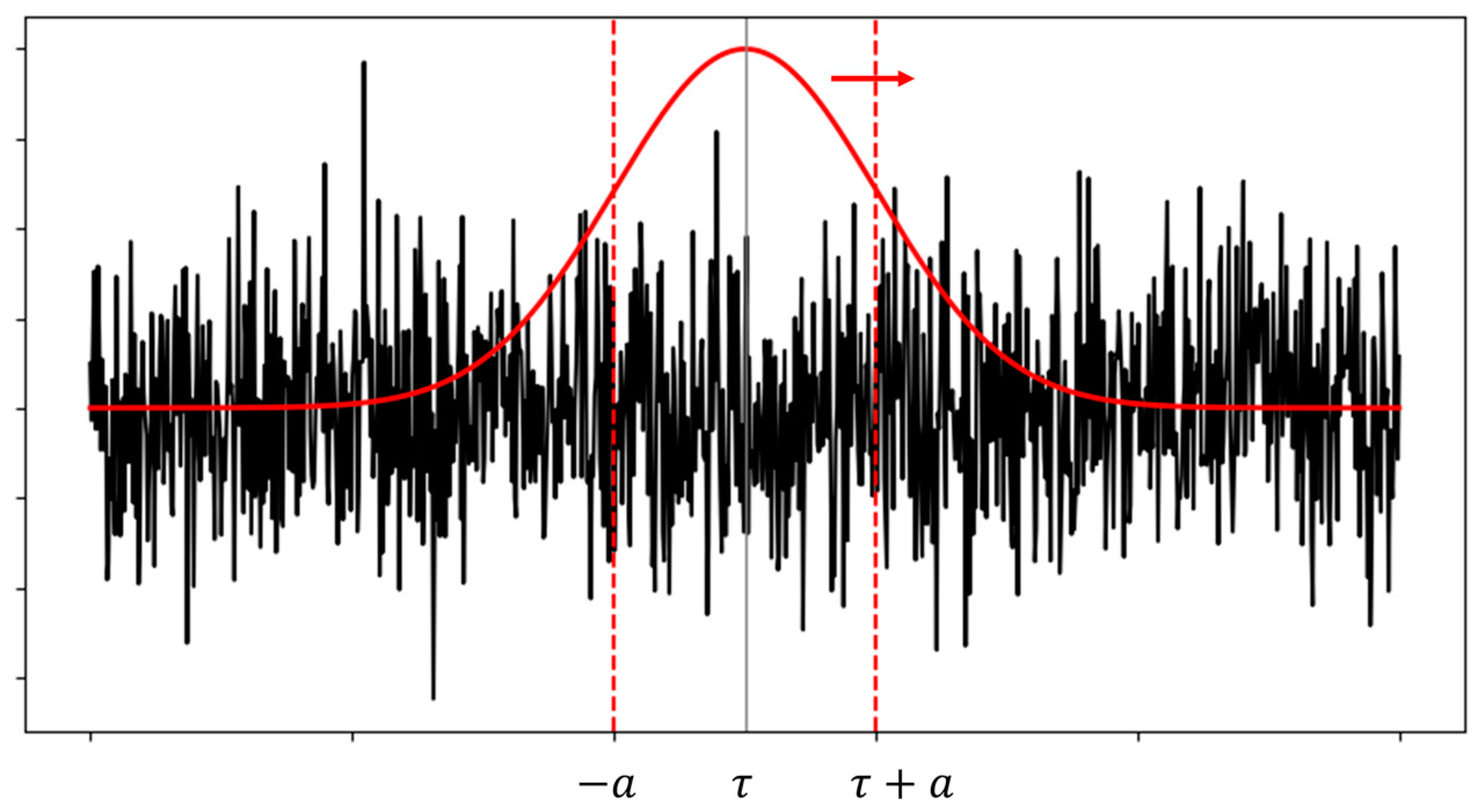
Figure 1. Illustration of the Gaussian window translation used in the STFT (adapted from [18]).
Vibration 07 00046 g001
Figure 2. Typical structure of a convolutional neural network (adapted from [4]).
Vibration 07 00046 g002
Figure 3. Example of a kernel (matrix in half) applied to extracting features from a bus image in a 2D network. The output highlights the lighter and more contrasting regions (adapted from [19]).
Vibration 07 00046 g003
Figure 4. ReLU and LeakyReL functions (with α = 0.1 for illustration purposes).
Vibration 07 00046 g004
Figure 5. Example of max pooling. Note the large reduction in dimensionality between input and output (adapted from [19]).
Vibration 07 00046 g005
Figure 6. Architecture of a convolutional neural network. Highlighted are the FC layer and the output layer (adapted from [8]).
Vibration 07 00046 g006
Figure 7. Control volume considered in the thermodynamic model (adapted from [17]).
Vibration 07 00046 g007
Figure 8. Pressure in one of the cylinders of the simulated thermodynamic model versus experimental data for different RPM (adapted from [27]).
Vibration 07 00046 g008
Figure 9. Vibration signals for each operating condition.
Vibration 07 00046 g009
Figure 10. STFT: (a) Normal condition, (b) pressure reduction in the manifold, (c) reduction in the compression ratio in the cylinders, and (d) reduction in the amount of fuel in the cylinders.
Vibration 07 00046 g010
Figure 11. CWT (a) Normal condition, (b) pressure reduction in the manifold, (c) compression ratio reduction in the cylinders, and (d) reduction in the amount of fuel in the cylinders.
Vibration 07 00046 g011
Figure 12. Original signals and signals added with noise.
Vibration 07 00046 g012
Figure 13. Examples of spectrogram with noise, normal condition: (a) 0%, (b) 10%, (c) 20%, (d) 40%, (e) 60%, and (f) 80%.
Vibration 07 00046 g013
Figure 14. Examples of scalogram with noise, normal condition: (a) 0%, (b) 10%, (c) 20%, (d) 40%, (e) 60%, and (f) 80%.
Vibration 07 00046 g014
Figure 15. General flowchart of the proposed methodology.
Vibration 07 00046 g015
Figure 16. Matrix with images for STFT for each condition and each noise level.
Vibration 07 00046 g016
Figure 17. Set of confusion matrix for STFT for each noise case, where: (1) is normal, (2) is pressure reduction, (3) is compression ratio reduction, and (4) is fuel reduction.
Vibration 07 00046 g017
Figure 18. Matrix with images for continuous wavelet transform (CWT) for each condition and each noise level.
Vibration 07 00046 g018
Figure 19. Confusion matrices for STFT for each noise case, where: (1) is normal, (2) is pressure reduction, (3) is compression ratio reduction, and (4) is fuel reduction.
Vibration 07 00046 g019aVibration 07 00046 g019b
Figure 20. First-layer filters for normal conditions.
Vibration 07 00046 g020
Figure 21. First-layer filters for pressure-reduction conditions in the manifold.
Vibration 07 00046 g021
Figure 22. First-layer filters for fuel-mass-reduction conditions.
Vibration 07 00046 g022
Figure 23. First-layer filters for conditions of reducing the compression ratio in a cylinder.
Vibration 07 00046 g023aVibration 07 00046 g023b
Table 1. Table of engine specifications used as a basis for data simulation ([17]).
DescriptionSpecifications
Stroke type4 strokes
Cylinders6 in line
Valve controlOn the head cylinder
Cylinder valves2 valves
Cylinder diameter105 mm
Piston stroke137 mm
Connecting rod length207 mm
Total displacement7118 L
Compression ratio16, 8:1
Inlet valve opening angle203°
Exhaust valve opening angle507°
Maximum torque and power900 Nm/191 kW
Rotation (in max. torque)1600 RPM
Ignition order1-5-3-6-2-4
Direction of rotationCounterclockwise (viewed from behind the wheel)
Rail pressure350–1400 bar
Cooling water temperature80–100 °C
Table 2. Test accuracy for each transform at the studied noise levels.
Signal NoiseCNN–STFTCNN–CWT
0%96.5%92.2%
10%81.1%84.3%
20%75.1%82.5%
40%71.5%70.4%
60%67.9%73.4%
80%57.0%73.5%
Disclaimer/Publisher’s Note: The statements, opinions and data contained in all publications are solely those of the individual author(s) and contributor(s) and not of MDPI and/or the editor(s). MDPI and/or the editor(s) disclaim responsibility for any injury to people or property resulting from any ideas, methods, instructions or products referred to in the content.