Sensitivity and Efficiency of the Frequency Shift Coefficient Based on the Damage Identification Algorithm: Modeling Uncertainty on Natural Frequencies

Abstract

Health surveillance in industries is an important prospect to ensure safety and prevent sudden collapses. Vibration Based Structure Health Monitoring (VBSHM) is being used continuously for structures and machine diagnostics in industry. Changes in natural frequencies are frequently used as an input parameter for VBSHM. In this paper, the frequency shift coefficient (FSC) is used for the assessment of various numerical damaged cases. An FSC-based algorithm is employed in order to estimate the positions and severity of damages using only the natural frequencies of healthy and unknown (damaged) structures. The study focuses on cantilever beams. By considering the minimization of FSC, damage positions and severity are obtained. Artificially damaged cases are assessed by changes in its positions, the number of damages and the size of damages along with the various parts of the cantilever beam. The study is further investigated by considering the effect of uncertainty on natural frequencies (0.1%, 0.2% and 0.3%) in damaged cases, and the algorithm is used to estimate the position and severity of the damage. The outcomes and efficiency of the proposed FSC based method are evaluated in order to locate and quantify damages. The efficiency of the algorithm is demonstrated by locating and quantifying double damages in a real cantilever steel beam using vibration measurements.

1. Introduction

Damage identification has drawn increasing interest in the sectors of aerospace, civil engineering and mechanical structures. The basic components of a structure make it very sensitive to damage that then require techniques for detecting damage using efficient methodologies. Damage can occur during manufacturing and in-service loading, such as fatigue and other object impacts. There are many methods to detect and determine the severity of damage based on Structure Health Monitoring (SHM). Many SHM methods, such as ultrasonic [1], guided wave [2], eddy current [3], scaling subtraction method [4,5,6] and nonlinear vibro-acoustic wave modulation technique [6], etc., have been developed to identify structural damage, which are used for various purposes. Although several Vibration Based Structure Health Monitoring (VBSHM) methods have been also proposed, they rely on vibration characteristics such as natural frequencies, mode shapes, etc. Some important VBSHM indicators are Damage Location Assurance Criterion (DLAC) [7], Multiple Damage Location Assurance Criterion (MDLAC) [8] mode shape curvature method [9] and the flexibility based method [10], which are effective and widely accepted in order to identify damage and their characteristics. Doebling et al. [11] presented a comprehensive review of different damage identification methods and health monitoring of structures from changes in the vibration characteristics. The damage conditions of the system can be described in five steps, as discussed in Rytter [12]. These steps are: (1) detection; (2) localization; (3) classification; (4) assessment; and (5) prediction. Dubey et al. [13] introduced a novel VBSHM strategy for geometry damage identification and size estimation using a damage library. The strategy was employed to estimate the size of rectangular geometry damage both numerically and experimentally in a tested cantilever beam. Vibration-based damage identification was used for a three-span continuous beam, a two-span steel grid [14] and a reinforced concrete beam [15], considering the effects of temperature variations. More recently, Toh and Park [16] provided a review applying machine learning algorithms for damage monitoring using vibration factors and interpretation of deep neural networks in order to guide further applications for structural vibration analysis.

In recent decades, natural frequencies have been used as an identification parameter for the detection, localization and quantification of damage. Salawu [17] acknowledged that natural frequency is a sensitive indicator to detect damage in the structure. Cawley and Adams [18] proposed a method based on the frequency shift that identifies the position of the damage in a plane structure. Narkis [19] analyzed the inverse problem for identification of crack position from frequency measurements. Silva and Gomes [20] proposed a technique using the frequency shift coefficient (FSC) to detect the crack size and position. Brincker [21] used a statistical analysis indicator to detect damage by changes in the measured natural frequencies. Kim et al. [22] developed algorithms to locate and quantify the damage through changes in the natural frequency. They addressed the damage sizing algorithms to quantify the size of the damage from a natural frequency perturbation. Armon et al. [23] introduced the rank ordering of natural frequency shifts for localization of damage. The development of a damage detection method by Zhang et al. [24] based on the frequency shift curve caused by auxiliary mass with both the natural frequency and mode shape information for cylindrical shell structures. Gillich et al. [25] performed crack identification based on natural frequency change. They established a mathematical model and signal processing algorithm, which can predict frequency changes for any boundary conditions with the identification of cracks on multi-span beams. Shukla and Harsha [26] presented a view that the change in natural frequency is an indication of cracks in the blade geometry. Keye [27] investigated the advantages of Finite Element (FE) model updating in association with a model-based method for structural damage localization. Gautier et al. [28] used a 4SID technique in combination with FE model updating procedure including an iterative domain partitioning procedure to localize damages. Dahak and Benseddiq [29] presented a normalized natural frequencies based method for a specific damage position in order to locate the damage in the cantilever beam. Therefore, the use of the unchanged frequency also gives us more accuracy when the damage is symmetric to the mode shape node. However, this method is independent of the beam dimension, material propriety or the severity of the damage.

Khiem and Toan [30] investigated natural frequency changes from the Rayleigh quotient that are derived for a clamped free beam with an arbitrary number of cracks. The authors compared natural frequencies calculated using the Rayleigh quotient and measured through an experiment, and they showed that the Rayleigh formula is a simple and consistent tool for modal analysis of cracked structures. Moreover, a crack detection procedure based on natural frequencies was introduced using Rayleigh quotient parameters. Le et al. [31] presented a method for the localization and quantification of simultaneous structural modifications based on the dynamic analysis in Euler Bernoulli beams with or without axial force. This method employs first-order estimation of frequency relative variation, which is derived from the continuous formulation. With this method, the damage position was identified, and then the damage was quantified by the relative variations of axial force, density and bending stiffness with nonlinear coefficients depending on the location of density and bending stiffness modifications. Khatir et al. [32] presented an approach for damage identification based on model reduction where an optimization algorithm is used to minimize the normalized difference between a frequency vector of the tested structure and its numerical model. Yam et al. [33] investigated the occurrence of damage in plate-like structures using sensitivities of static and dynamic parameters. The authors suggested two damage indices for damage identification based on the curvature mode shape and the strain frequency response function.

Serra et al. [34] proposed a strategy to detect and localize damage using various classical indicators by testing different damage cases. Eraky et al. [35] focused on the damage index method (DIM) as a tool for determining elemental local damage that occurred in beam and plate structures. However, this technique depends on an experiment based on comparing modal strain energies at different degradation stages. More recently, Serra and Lopez [36] presented a combined modal wavelet strategy. They compared it with the most frequently used indicators and widely studied methods in order to identify the damages. The performance of each method is evaluated and the capacity to detect and localize damage are tested through different cases. Hu et al. [37] used a statistical based damage-sensitive indicator for the health monitoring of a wind turbine system by considering environmental and operational influences on the structural dynamic properties. Karbhari and Lee [38] used a dynamic structural analysis to detect damage by applying a cosine based indicator and a model assurance criterion for an eight degrees of freedom structure in order to perform effectively in identifying damages to the structure.

Finally, several studies on damage identification are based on the use of the Frequency Response Function (FRF) and Particle Swarm Optimization (PSO). Porcu et al. [39] proposed an FRF-curvature based technique (FRF-curvature damage indicator) for damage identification in structural components and tested it both experimentally and numerically. The authors show that the FRF curvature method is more effective, compared to other methods (e.g., natural frequencies, mode shapes or mode-shape curvatures). Furukawa and Kiyono [40] introduced a technique for the detection of damage in structures that use FRF data as generated from the harmonic excitation force. The method is based on the fact that structural damage usually causes a decrease in structural stiffness and an increase in structural damping, thereby producing changes in vibration characteristics. Mohan et al. [41] used FRFs with the help of the PSO technique for damage detection and quantification. The robustness and efficiency of this method are acknowledged after comparing the results between two methods: Genetic Algorithm (GA) and PSO.  Khatir et al. [32] presented an inverse problem with an optimization algorithm for minimizing the cost function for damage detection and localization. They implemented FEM with PSO and GA to perform the inverse computations. Huang et al. [42] proposed an optimization approach, known as bare bones PSO with a double jump, in order to come up with a solution for the damage identification. The authors implemented a $l_1$ regularization function for detecting damage cases especially in a noisy environment. Li et al. [43] used the standard PSO-FEM to compare the performance of fitness functions using natural frequencies. Later, the authors proposed an algorithm based on multi-component PSO with a cooperative leader learning mechanism for structural damage detection and further compared with other recent optimization algorithms [44]. Alamdari et al. [45] implemented FRFs in a damaged structure and a damage sensitive shape was generated by taking the derivatives of operational mode shapes with the anti-symmetric extension and shape signals that are normalized at different natural frequencies. Moreover, these studies focused on frequency-based damage detection strategies.

From this literature review, it is found that several VBSHM techniques using natural frequencies have been considered for structural damage detection. A few techniques (wavelet transform, artificial neural network, etc.) have shown reliable results with the consideration of measurement errors or uncertainties. As we know, uncertainty or noise is always present on natural frequencies and other modal parameters that can lead to inadequate structural damage detection. An FSC-based algorithm is introduced, and different cases were investigated with or without consideration of uncertainty or measurement errors on natural frequencies. The algorithm was employed by minimizing FSC using PSO, where damages are localized and quantified by updating the FE model from the FSC algorithm that is based on natural frequency shifts. The damage identification technique was performed based on bending stiffness reduction using the FE models. For that, 2D FE models were developed for the healthy and damaged beams, and numerical damage cases were built artificially to test the proposed algorithm. The difference between healthy and damaged models were weighted depending on the shift of natural frequencies. It means the damage localization and quantification can be accurate based on the sensitivity of frequencies shift to the damage states. The paper is intended to further investigate the efficiency of the FSC based method by evaluating the identification capacity in uncertain damaged cases. The FSC-based method is demonstrated by testing a real beam that has been double damaged using an experimental test.

The paper is organized as follows: Section 2 illustrates the modeling of the beams and bending vibration theory; Section 3 presents the proposed damage identification strategy using FSC minimizing algorithm; Section 4 shows different numerical examples in order to verify the effectiveness of the method and discussion about the influencing factors, i.e., influence of the damage positions and severity. The artificially damaged cases are investigated in order to localize and estimate the severity along the cantilever beam. The effect of the modeling uncertainty on natural frequencies is considered and the test cases are examined by considering different noise levels; Section 5 shows a simple laboratory experiment for the vibration measurements in order to find positions and severities of damage in a real beam structure.

2. Beam Vibration Theory

It is assumed that the simplest damage detection problem can be explained by testing beams using a linear equation of motion with undamped free vibration. The equation of motion for free vibration analysis of an Euler–Bernoulli beam is given by:

$$M\left(x\right)\frac{{\partial }^{2}w(x,t)}{\partial t^2}+\frac{{\partial }^2}{\partial x^2}\left(EI\left(x\right)\frac{{\partial }^{2}w(x,t)}{\partial x^2}\right)=0,$$

(1)

where $w(x,t)$ is the transverse deflection of the beam base axis, $M\left(x\right)$ is the mass per unit length of the beam, $EI\left(x\right)$ is the bending stiffness of the beam. Here, a harmonic time dependency is assumed, and the cantilever beam is taken into consideration that is clamped in x = 0 and free in $x=L$; then the solution would satisfy $u^{″}\left(L\right)=u^{‴}\left(L\right)$ = 0 and $u^{\prime }\left(0\right)=u\left(0\right)$ = 0. To calculate the normal modes we have to consider the linear homogeneous equation related to Equation (1). Then, the differential equation of eigenvalue problem is written as:

$$\left(EI\left(x\right){\varphi }_n^{″}\left(x\right)\right)″-{\lambda }_{n}M\left(x\right){\varphi }_n\left(x\right)=0,$$

(2)

where $\sqrt{{\lambda }_n}$ and ${\varphi }_n$ are the associated natural frequencies and the normal modes. In order to determine the Rayleigh quotient using normal mode shapes $\left({\varphi }_n\right)$ of the undamped problem the normal modes $\left({\varphi }_n\right)$ are considered as the functions, represented by ${\varphi }_n\left(x\right)$, which is the square integral on $\left[0L\right]$ (i.e., ${\varphi }_n\left(x\right)\in C^2(0,L),$ and $C^2$ denotes for a square-integrable function) as well as ${\varphi }_n^{{}^{\prime }}$ and ${\varphi }_n^{″}\left(x\right)$. Multiplying Equation (2) by any function $u\left(x\right)$ with $u\in C^2(0,L)$ and taking the partial integration, we obtain:

$${\int }_0^L\left(EI\left(x\right){\varphi }_n^{″}\left(x\right)u^{″}\left(x\right)\right)″-{\lambda }_{n}M\left(x\right){\varphi }_n\left(x\right)u\left(x\right))dx+bc=0,$$

(3)

where $bc$ is a vanishing term representing the boundary conditions. The quantity of $bc$ is equal to zero for any function $u\left(x\right)$ by verifying the same boundary condition as the modes. Similarly, natural frequency (Hz) calculation for the beam is given by:

$$f_n=\frac{\sqrt{{\lambda }_n}}{2\pi },$$

(4)

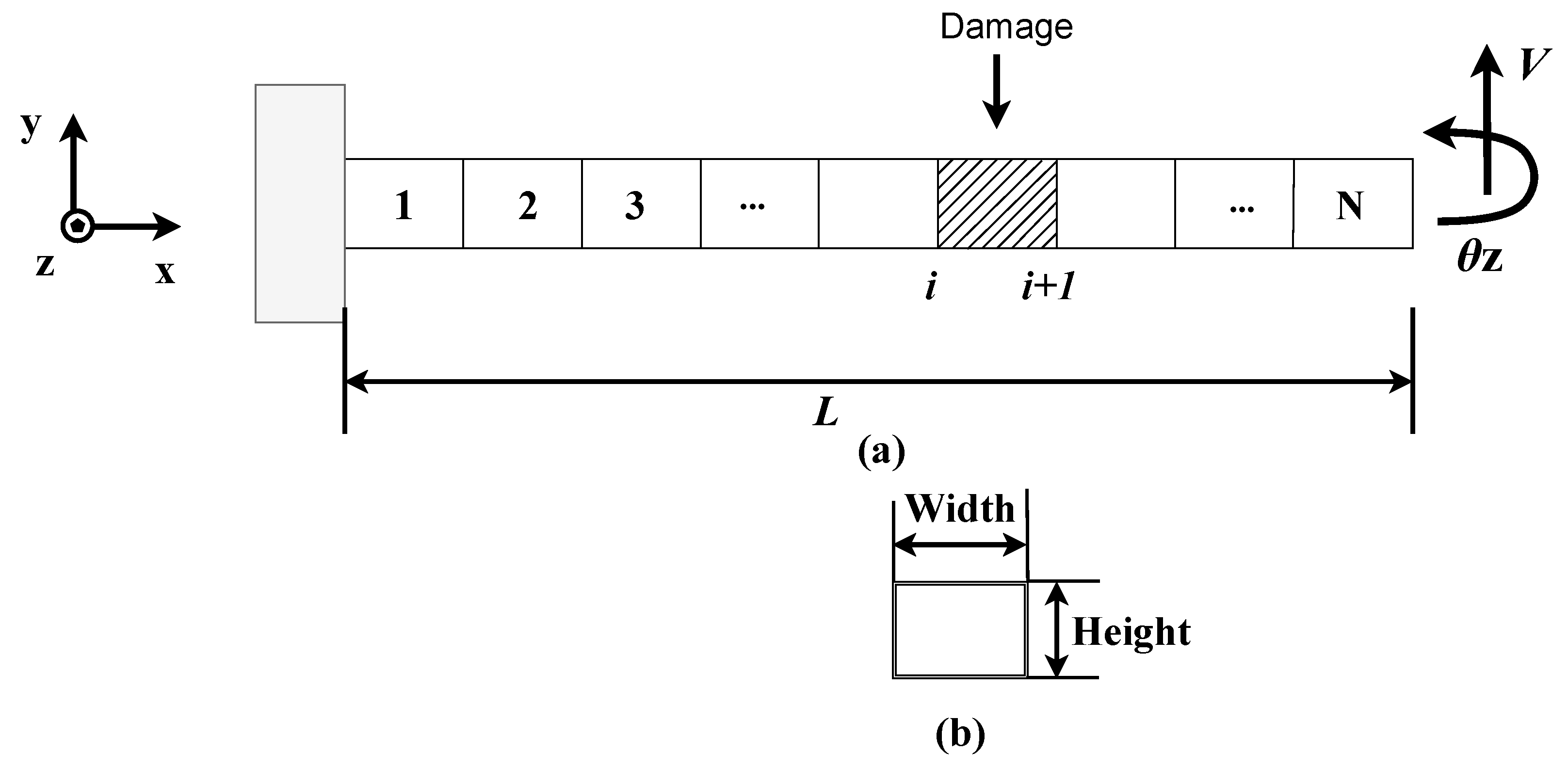
2.1. 2D Finite Element Models of Beam

The studied model is considered to be an Euler–Bernoulli cantilever beam with a uniform cross-section area with 2D healthy and damaged FE beam models. The 2D FE beam models are discretized in N elements and $N+1$ nodes. Figure 1 shows a 2D FE damaged model of a cantilever beam and its cross-section area. Each node of the FE models has two degrees of freedom, a vertical translation V and a bending rotation ${\theta }_z$.

Natural frequencies and mode shapes may be obtained by solving an eigenvalue problem from the FE model as described by the following equation:

$$(\left[K\right]-\left({\omega }_i^2\right)\left[M\right])y_i=0$$

(5)

where $\left[M\right]$ is the $n\times n$ mass matrix of the system, and $\left[K\right]$ is the $n\times n$ stiffness matrix of the system, where ${\omega }_i$ are natural frequencies and $y_i$ are modal shapes.

Here, the damage is assumed at position $x_l$ within node i to $i+1$ of the beam. If a defect is introduced in a beam structure, it reduces the stiffness of the beam structure at a particular element.

2.2. Numerical Modeling of Damage

In the 2D FE model, damage severity is represented by an elemental stiffness reduction coefficient ${\alpha }_i$, which is the ratio of the stiffness reduction to the base stiffness. The stiffness matrix of a numerical damaged FE model is defined as the sum of elemental matrices multiplied by the reduction coefficient:

$$\left[K_d\right]=\sum _{i=1}^N(1-{\alpha }_i)\left[K_e\right]$$

(6)

where $K_d$ is the global stiffness matrix for a damaged beam, $K_e$ is the elemental stiffness matrix, N is the number of elements and ${\alpha }_i$ is a reduction coefficient, which varies from 0 to 1 for the damaged structure. A value of ${\alpha }_i$ = 0 indicates a healthy element.

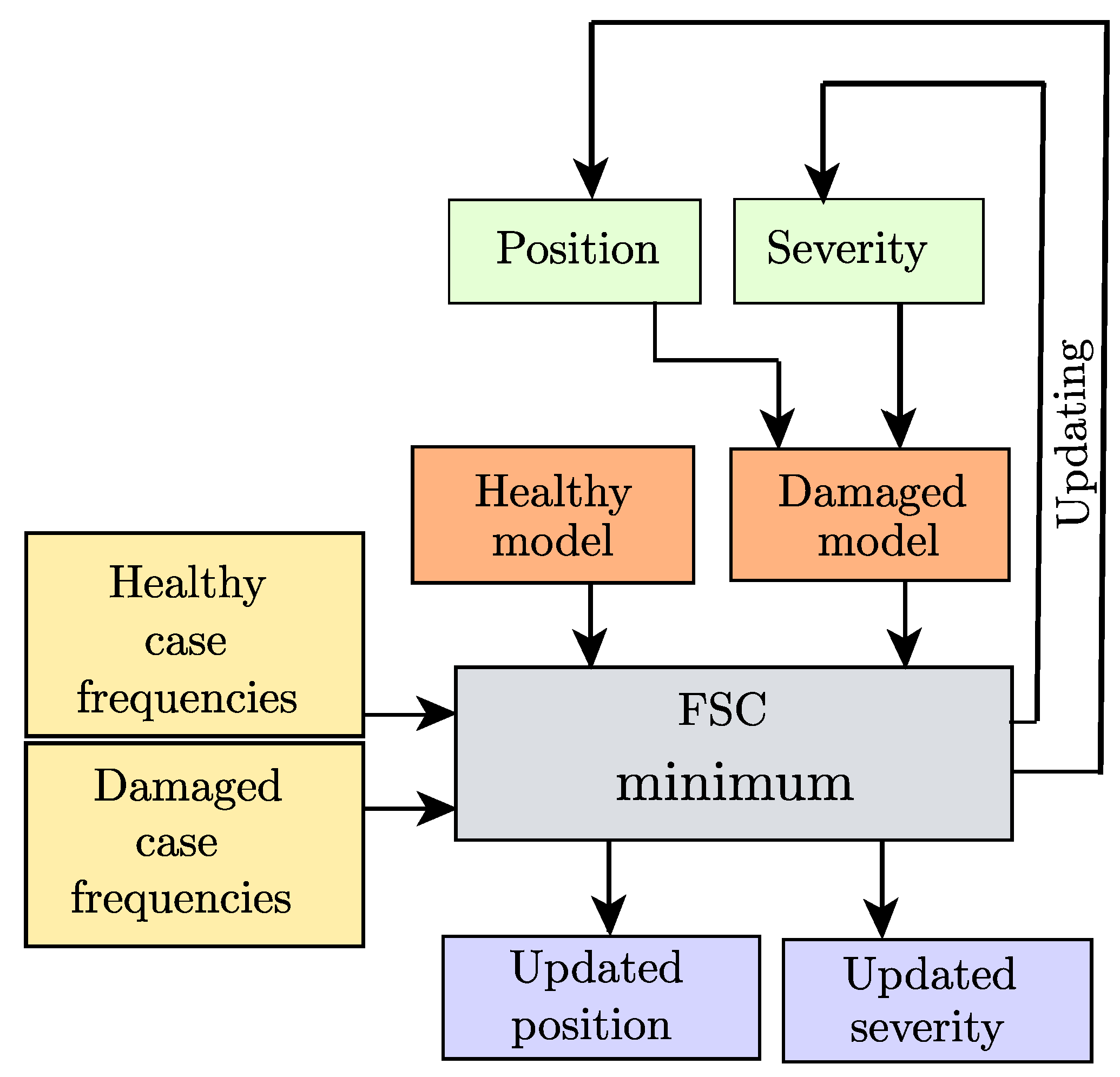
3. Proposed Damage Identification Strategy

3.1. Objective Function

Damage positions and severity are estimated using an FSC based method. FSC is cited by Doebling et al. [11], and was first presented by Silva and Gomes [20] for damage identification problems. The indicator requires experimental measurements or numerical solutions for the frequency shifts as a function of position and size of the damage. The FSC indicator is written as:

$$\mathrm{FSC}=\sqrt{\frac{1}{n}\left|\sum _{i=1}^n\left(\frac{{\left\{{\Gamma }_i\right\}}_X-{\left\{{\Gamma }_i\right\}}_A}{{\left\{{\Gamma }_i\right\}}_X}\right)\right|}$$

(7)

$$\mathrm{and}{\Gamma }_i=\frac{f_i^d}{f_i^h}$$

where n is the total number of modes, X is the tested case, A is the updating model, $f_i^u$ is the unknown beam natural frequencies, $f_i^h$ is healthy beam natural frequencies and i denotes modes indices. Here, considering the vectors of $l=[l_j\dots l_p]$ and $\alpha =[{\alpha }_0\dots {\alpha }_p]$, these vectors are the set of testing positions (measured from the clamped area to the end of the beam) and the corresponding stiffness reduction in each position for the unknown defect, respectively.

The FSC value arrives at zero or close to zero during the identification of the damage position and severity using natural frequencies of healthy and damaged beams. For the noisy and real experimental cases, the values fall close to zero. FSC values are found for damaged cases, ranging from 1 to 90% stiffness reduction at all beam positions. Overall, the minimized value from FSC indicates corresponding damage positions and severity.

The coefficient is suitable for locating and quantifying damages from the beginning to the end of the beam, as is further demonstrated in later sections. With small amounts of damage, the results are very precise; in other words, the FSC is capable of damage assessment for cases ranging from small to large damage.

3.2. Proposed Strategy and Minimization Problem

In this section, Figure 2 shows the flowchart of the proposed damage identification strategy. FSC is used as a function of beam position and elemental stiffness reduction. The damage is compared between the healthy and damaged FE models using the frequency shift approach. Here, four beam models with the same beam properties are used for the FSC-minimization purpose. The damaged and healthy beam natural frequencies are measured, which are then used for comparison with other healthy and FE updating damaged models. The aim of FSC minimization is to identify the best-fit values of positions and severities for the tested damaged cases.

The solutions of the minimization problem are obtained using Particle Swarm Optimization (PSO) (Kennedy and Eberhart) [46]. Many other methods can be used, but the principal purpose behind this choice is to find global solutions and to evaluate or approximate the solution of the cost function, i.e., the FSC. PSO is implemented by the particlewarm() function in the MATLAB global optimization toolbox and is adequate for solving the minimizing problem. The application of the FSC algorithm with PSO directly reveals solutions as parameters of the damage assessment steps as if the initial damage has already been detected.

There are several parameters in PSO, i.e., the swarm size, number of iterations, inertia weight, learning factors, etc. We use default values for most of the PSO parameters because it allows us to obtain the correct results. In FSC minimization, only the swarm size and number of maximum iterations with values of 20 and 100 are explicitly specified.

3.3. Steps for Damage Identification Procedure

The proposed algorithm for damage assessment is detailed in the following steps:

1. Generate a damaged case with the reduction in bending stiffness ranging from 0.01 to 0.99. This corresponds to an experimental real damaged case or unknown case.

2. Estimate the natural frequencies for the first n-bending vibration modes by developing FE models of healthy and damaged states. It leads to the vectors of healthy $\left(H_f\right)$ and damaged beam natural frequencies $\left(D_f\right):[f_1\dots fn]$. In order to simulate measurement imprecision, we consider introducing a perturbation to the set of natural frequencies for the case being impaired.

3. Use the FSC function and the minimization strategy for each set of tested natural frequencies and update the FE model for generic damage.

4. Consider the updated parameters as the damage parameters. In the case of perturbations, find the mean and standard deviation of different identified damage parameters as the final results.

3.4. Modeling Uncertainty on Natural Frequencies

Measurement errors and sensor noise can be cause of uncertainties in the experimentally determined modal parameters, and it is impossible to completely remove these uncertainties from the measured data. In this way the proposed algorithm is tested for numerically generated uncertain cases, i.e., cases with incorrectly estimated natural frequencies. In the case of a damaged beam, uncertain or noisy conditions are introduced on the natural frequencies with the addition of percentage noise levels and considered Gaussian distributed random variables. To generate the uncertainty on natural frequencies the following equation is adopted:

$${\overline{\omega }}_i^d={\omega }_i^d(1+\eta {\gamma }_i)\mathrm{and}i=1,2\dots ,n$$

(8)

where ${\overline{\omega }}_i^d$ is ith damaged beam natural frequency after noise addition, $\eta$ is the percentage of noise and ${\gamma }_i$ is a Gaussian random number between −1 to 1 that is different for each i. When uncertainties are considered in the rest of the article, we have assumed noise levels of $\eta$ = 0.1%, 0.2% and 0.3% in natural frequencies of the tested beam.

4. Numerical Validation of Method

In this section, anFSC minimizing algorithm is considered, and various numerical cases are evaluated to determine the efficiency of the proposed identification procedure. The FE models of the cantilever beam structure are developed in order to extract the dynamic characteristics.

To examine the FSC method, various numerically introduced damaged cases are selected and simulated, where the position of damage and size are varied.

4.1. Numerical Beam Model

The Euler–Bernoulli cantilever beam is discretized using 100 elements, as described in Section 2.1, and its material and physical properties are given in 

Table 1. Beam dimensions and properties.

Beam Properties	Value
Length (L)	1000 $\mathrm{mm}$
Width (W)	25 $\mathrm{mm}$
Thickness (T)	5.4 mm
Young’s modulus (E)	210 GPa
Poisson’s ratio (v)	0.33
Mass density ($\rho$)	7850 $\mathrm{kg}/{\mathrm{m}}^3$

. Modal parameters for healthy and damaged beams are generated using MATLAB.

First, it is important to update Young’s modulus of the 2D FE model in order to closely match the natural frequencies of the 2D FE healthy model to a healthy real experimental beam. To determine the updated Young’s modulus, a maximization problem is formulated that uses the inverse of the statistical error on implementing the natural frequencies of the 2D numerical and experimental healthy beam. The function of Young’s modulus updating $\left(E\right)$ is as follows:

$$E=\mathrm{Argmax}\left(\frac{1}{\sqrt{\frac{1}{m}\left|{\sum }_{i=1}^m{\left(f_i^{2D}-f_i^h\right)}^2\right|}}\right)$$

(9)

where $f_i^{2D}$ represents natural frequency of updating 2D FE beam model and $f_i^h$ represents identified natural frequency of healthy experimental beam. Equation (9) is employed to obtain best-fit maximized value of updated Young’s modulus for 2D FE cantilever beam model. The Young’s modulus of primary 2D FE model (E = 210 GPa) must be minimized on the basis of the modeling errors between the natural frequencies of the real structure and the 2D FE healthy model. The updated Young’s modulus will be then used for damage identification purpose.

For 2D FE Model, Young’s modulus is taken into account by considering it as an updating parameter. A set of vector parameter is generated, and the Young’s modulus value of steel beam is updated from an initial value of 210 GPa to 189.26 GPa using Equation (9), with a maximum value of 0.863.

In addition, the first seven healthy beam natural frequencies (experimental and numerical) are listed in 

Table 2. Numerically and experimentally (see Section 5) measured natural frequencies of the healthy cantilever beam.

Healthy Beam	Natural Frequencies (Hz)
	1	2	3	4	5	6	7
Experimental	4.27	26.33	73.26	142.34	240.12	355.66	499.66
2D FE Model (updated E = 189.26 GPa)	4.20	26.35	73.77	144.56	238.96	356.97	498.57
Errors (%)	0.70	0.08	0.69	1.54	0.49	0.36	0.22

. An experimental beam test in order to obtain natural frequencies is detailed in Section 5. Here, relative errors between the natural frequencies of the real healthy beam and the 2D FE healthy beam, have been reported in Table 2. The mean error value is 0.687 Hz between the experimental natural frequencies and the numerical updated natural frequencies.

Moreover, the reduction in CPU time is an important factor in the identification of damages. For that, seven natural frequencies are considered to be appropriate for the identification of damages that may occur in the structure. During the Young’s modulus updating procedure, the seven lowest frequencies are assumed to be sensitive enough to classify the damage position and severity using an FSC. Here, two significant digits after the decimal in the natural frequencies proves sufficient for the algorithm to solve the minimization problem for determining the damage parameters.

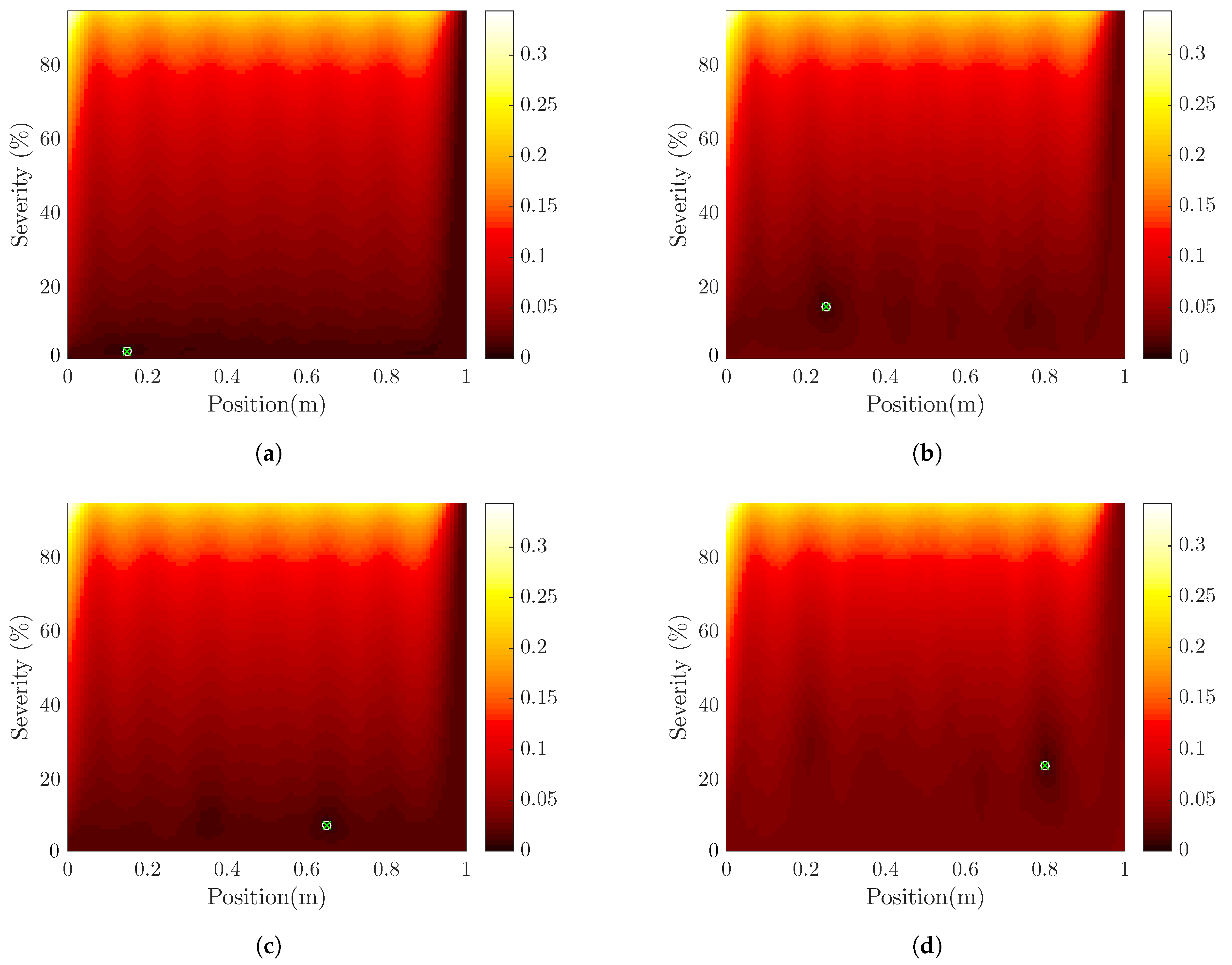
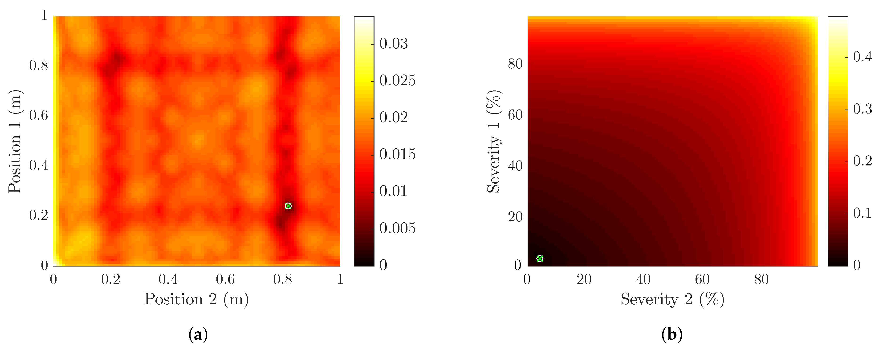
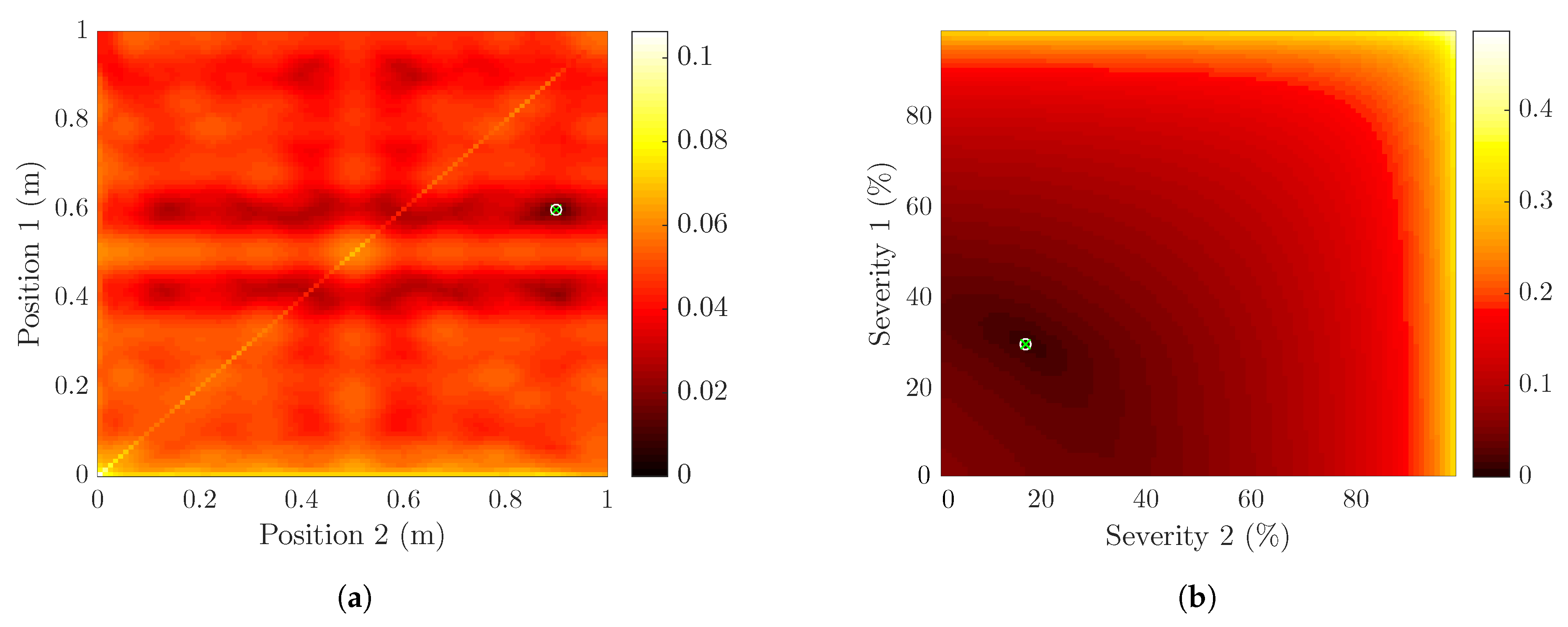
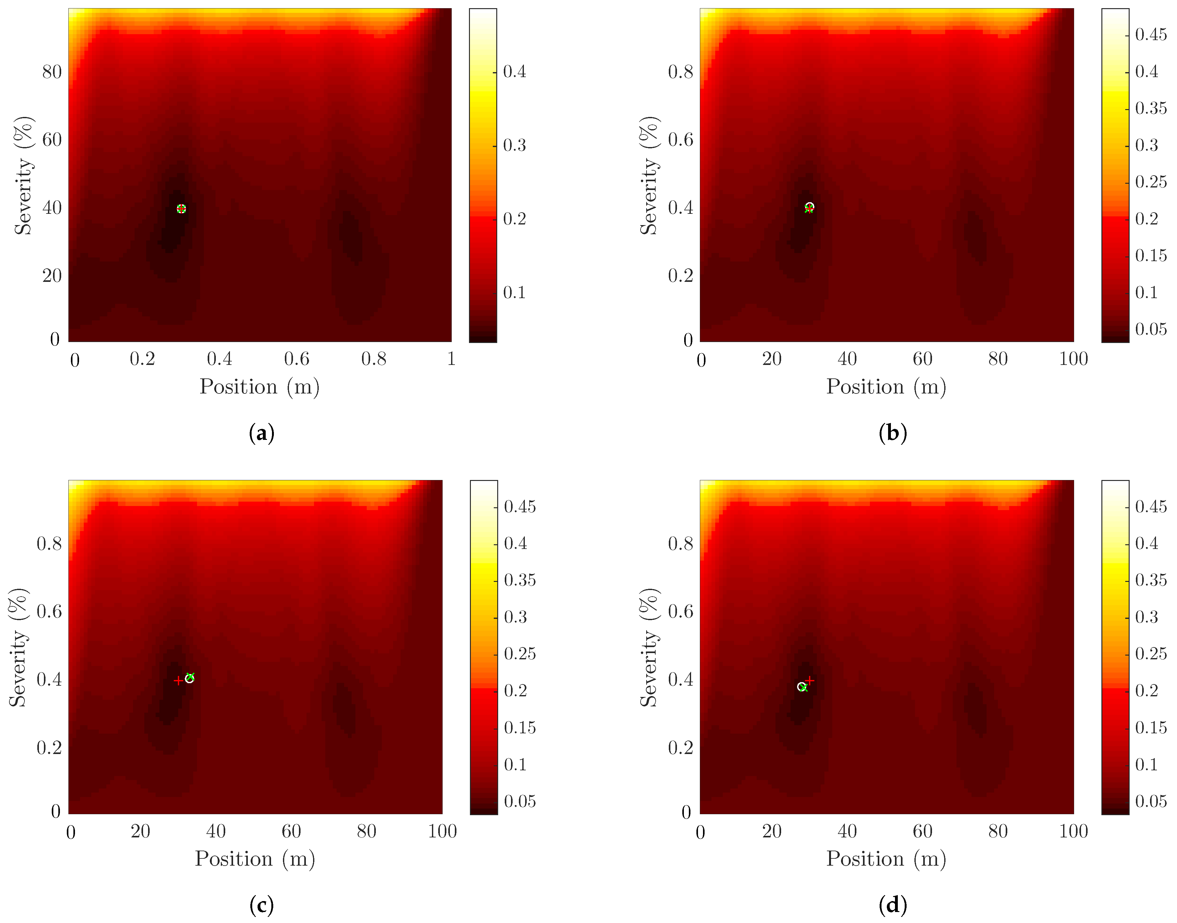
4.2. Localization and Quantification of Single Damage

Further identification of damage is considered in order to highlight the efficiency of the proposed FSC minimizing algorithm. In this part, FSC is used for localization and estimation of artificially introduced 2D damaged cases.

Four single and artificially damaged cases are developed in the 2D FE cantilever beam model. For a given case, the damages are introduced in different positions from the clamp to the end sites of the cantilever beam. These cases are given (a) near the clamped site at 0.15 m, (b) before the mid-site at 0.25 m, (c) after the mid-site at 0.65 m and (d) near the end-site at 0.80 m with 2%, 15%, 8% and 24% along the beam, respectively. Single damages cases and their first natural frequencies are reported in 

Table 3. Single damaged cases and numerically identified natural frequencies of damaged beams.

Damaged Cases	Natural Frequencies (Hz)
	1	2	3	4	5	6	7
(a) $x_l=$ 0.15 m, ${\alpha }_l=$ 2%	4.20	26.34	73.77	144.55	238.92	356.90	498.51
(b) $x_l=$ 0.25 m, ${\alpha }_l=$ 15%	4.20	26.34	73.68	144.35	238.88	356.90	497.89
(c) $x_l=$ 0.65 m, ${\alpha }_l=$ 8%	4.20	26.35	73.73	144.46	238.92	356.93	498.23
(d) $x_l=$ 0.80 m, ${\alpha }_l=$ 24%	4.20	26.33	73.59	144.04	238.37	356.79	492.47

.

In damaged cases, single damages are assessed to demonstrate the efficiency of the approach as shown in Figure 2. The proposed technique (see Section 3.2) and algorithm (see Section 3.3) are implemented to classify the position and severity of the damage. The technique is evaluated using the FE updating strategy of bending stiffness within 2D vs. 2D FE models. Based on FSC, the 2D healthy and damaged case natural frequencies are extracted, performed with other healthy 2D and stiffness updating damaged model natural frequencies in order to minimize FSC.

At the same time, the PSO (as implemented by Particleswarm() from MATLAB global optimization toolbox) with the FSC algorithm is then used to locate and estimate the severity of the damage using the FSC objective function, as defined in Equation (7). FSC value arrives zero or close to zero. Here, Particleswarm() function works as part of the algorithm to find optimal global solutions (position and severity).

Figure 3 shows the identification of the given single damaged cases (see Table 3). FSC is displayed as a function of the position and severity. The white circles denote the real damaged parameters. Here, cross symbols are obtained by minimizing the FSC by using the PSO function, and the color bars signify the color value for FSC. In terms of the results, the damage position and severity values a were obtained at 0.15 m, 0.40 m, 0.70 m and 0.80 m with 2%, 15%, 8% and 24%, respectively. A low value of FSC indicates that the attempted damaged case and unknown case are similar from the FSC point of view. We thus present the FSC values for increased understanding. The minimum value can indicate the damage parameters, especially if it is zero or close to zero. This means that the algorithm is well adapted for localizing and estimating damage.

In Figure 3a, it is found that minor damage can be better estimated when using more precise measurements. Indeed, FSC shows (see Figure 3) that the position and severity of the damage are correctly assessed and does not create uncertainty regarding the actual position and severity of the damage. It is noted that the processing time is approximately 10 s when using the PSO function. To summarize, FSC has solid performance in these cases with a low computational time. To verify the accuracy of the FSC algorithms, position and severity corresponding to the FSC minimum values are considered to be damage identification parameters that are precisely consistent with the actual position and severity values of the damaged cases.

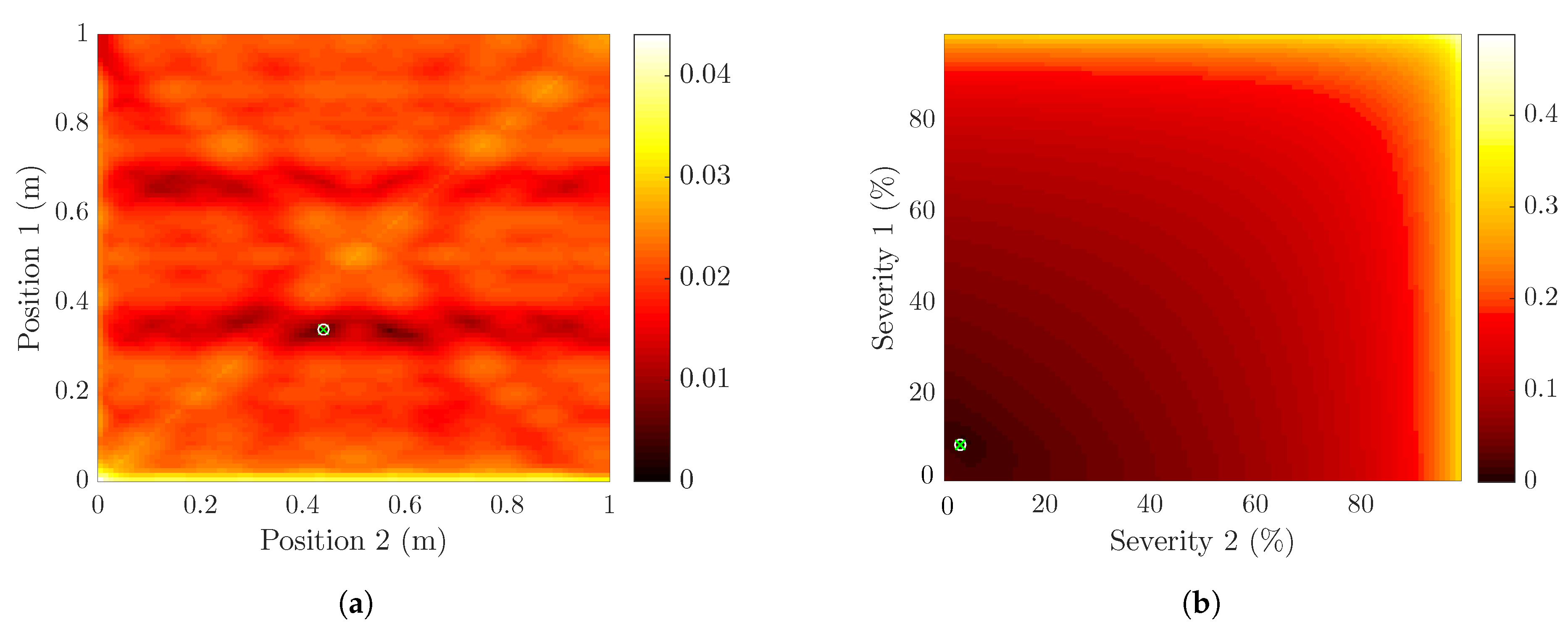
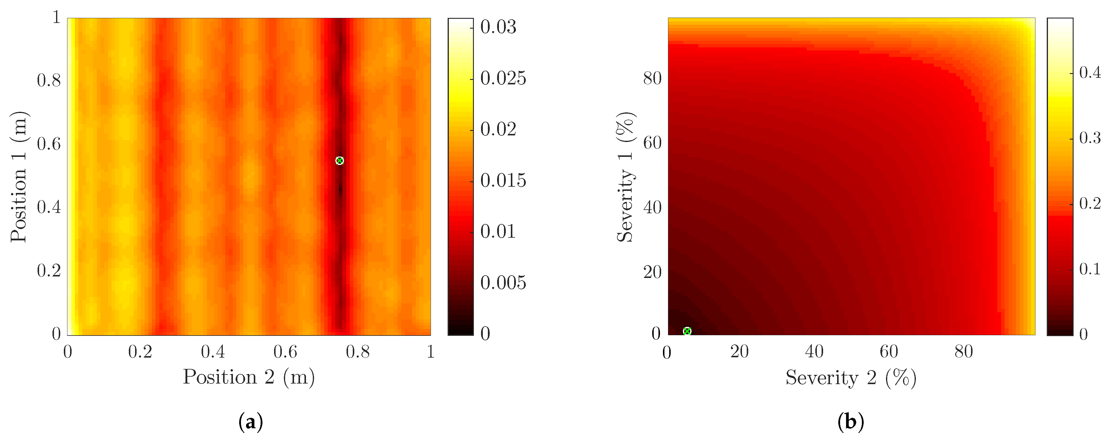
4.3. Localization and Quantification of Double Damages

Specific numerical damaged cases, each with two damages, will be assessed along the cantilever beam structure. Double-damaged cases are generated numerically by the reduction of bending stiffness of two beam elements.

In the FE beam, the damaged sites were selected close and far from each other, where the amount of damage ranges from lower to higher percentages. In terms of position and stiffness reductions, double-damaged cases are given (a) at 0.1 m and 0.2 m with 7% and 2%, (b) at 0.50 m and 0.90 m with 15% and 35%, (c) at 0.45 m and 0.55 m with 15% and (d) 0.10 m and 0.15 m with 60% and 68%, respectively. Different damaged sites with two damages are introduced and, for each, their natural frequencies are reported (see 

Table 4. Two damaged cases and their numerically identified natural frequencies.

Damaged Cases	Natural Frequencies (Hz)
	1	2	3	4	5	6	7
(a) $x_l=$ 0.24 m, ${\alpha }_l=$ 3%,
$x_m=$ 0.82 m, ${\alpha }_m=$ 5%	4.20	26.34	73.73	144.43	238.81	356.87	498.47
(b) $x_l=$ 0.60 m, ${\alpha }_l=$ 30%,
$x_m=$ 0.90 m, ${\alpha }_m=$ 17%	4.20	26.24	73.59	144.30	237.70	356.27	495.61
(c) $x_l=$ 0.34 m, ${\alpha }_l=$ 9%,
$x_m=$ 0.44 m, ${\alpha }_m=$ 4%	4.20	26.33	73.70	144.51	238.77	356.61	498.35
(d) $x_l=$ 0.55 m, ${\alpha }_l=$ 1%,
$x_m=$ 0.75 m, ${\alpha }_m=$ 6%	4.20	26.34	73.72	144.46	238.93	356.90	498.25

) solving the eigenproblem using FE.

In order to minimize FSC, the numerical seven natural frequencies of the damaged beam were used as inputs. Natural frequencies are extracted from the double-damaged beam (see Table 4) and are fed to the algorithm based on FSC. There are four parameters (position 1, position 2, severity 1 and severity 2) unknown to identify for two damage identification, and two stages are followed to represent identified damaged positions and severities and the variations of the FSC on Figure 4, Figure 5, Figure 6 and Figure 7. For a better understanding and a comprehensive representation, we will split the parameters space in two. First: assuming a certain percentage of severity for two damages, FSC is represented as a function of the beam positions. Second: assuming the positions of two damages, FSC is displayed as a function of severity. Lastly, cross symbols and circles signify global minimized values. However, cross symbols are obtained using the PSO function with the global FSC minimization. In order to classify the damages in terms of parameters (positions and severities), vectors of four parameters are defined in the algorithm. Next, PSO was used to find the global minimum on the parameters space. Accordingly, there will be only one global minimum indicating the associate presence of impaired parameters, which is obtained by modal analysis using FSC between healthy and damaged states. Note that the two damages may happen to have the same position; in this case, we add the severity and apply the stiffness reduction to a single element.

Positions and severity of double damaged cases (a) and (b) are identified, and shown in Figure 4 and Figure 5, where, Figures (a) and (b) are two representations of the same 4+1D space. FSC is plotted as a function of positions and severity. These examples are localized at far distances from each other along the beam, while levels of severity are estimated from lower to higher percentages. Double-damaged case (a) is identified at positions 0.24 m and 0.82 m with 3% and 5% damage severity. Similarly, double-damaged case (b) is found at the end side of the beam, where damages are localized at 0.60 m and 0.90 with 30% and 17% severity, respectively. The PSO solver is used to obtain an output of minimizing parameters that are denoted by cross symbols. However, these symbols are perfectly overlapping to circles as these circles are defined for real parameters of artificial damaged cases. Hence, damages are identified in the end sites of the beam since they are located well apart from each other. Figure 4b shows that the low levels of damage severity are quantified, where damages are located far from each other. It also indicates that the algorithm is well-suited to identify the small double damages, as well as if they are located far away from each other.

Other subsequent double damaged cases (c) and (d) are explored at various beam positions with dissimilar stiffness reductions using FSC based minimizing algorithm. Similarly, the algorithm with the PSO function is used to obtain outputs of the minimizing parameters. Figure 6 and Figure 7 show the identification of double damaged cases (c) and (d). These two instances are achieved as either low (9% and 4%) or high (60% and 70%) levels of impaired severity at positions (0.34 m and 0.44 m) and (0.10 m and 0.15 m), respectively. These identifications also demonstrate that the algorithm is suitable for identifying small damages and also if the damage is close together. This reveals that the algorithm has a close correlation between artificially simulated damaged cases and the 2D updating FE reference model.

In order to localize and estimate more than two damages, the condition should be assessed by increasing the number of parameters in order to solve the minimization problem. It is important to note that there is a relationship between input and output parameters throughout the minimization problem.

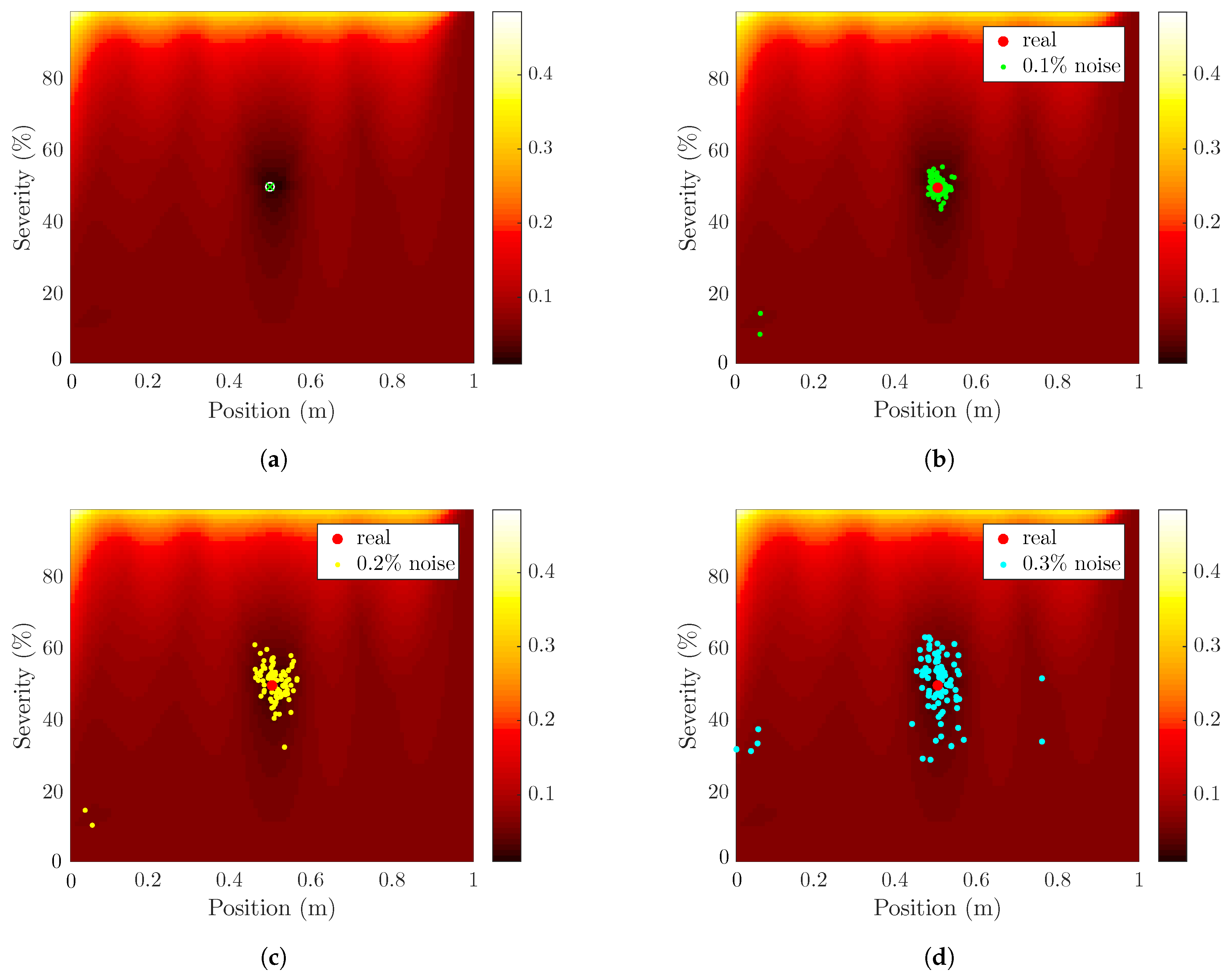
4.4. In the Case of Modeling Uncertainty on Natural Frequencies

Numerical damaged cases and their identified natural frequencies are listed in

Table 5. Damaged cases and numerically identified natural frequencies of damaged beams.

Damaged Cases	Natural Frequencies (Hz)
	1	2	3	4	5	6	7
(a) $x_l=$ 0.30 m, ${\alpha }_l=$ 40%	4.18	26.31	73.35	144.21	238.86	354.98	496.20
(b) $x_l=$ 0.50 m, ${\alpha }_l=$ 50%	4.19	26.08	73.77	143.16	238.94	353.60	498.51

. These cases will be tested by the proposed damage identification to investigate the sensitivity of FSC. Here, uncertainties of natural frequencies are generated from Equation (8) by adding perturbations of 0.1%, 0.2% and 0.3%.

Figure 8 indicates the identification of the damaged case (a) ($x_l$ = 0.30 m and ${\alpha }_l$ = 40%) with and without consideration of the perturbation in natural frequencies, while the natural frequencies for the tested case (a) are listed in Table 5. FSC is plotted as a function of positions and severity, and the plus symbols indicate the actual damage position and severity depending on the impaired case. White circles (obtained by the FE updating strategy using FSC), green cross symbols (obtained by PSO using FSC) and color bars represent the lowest minimized values. The damage is perfectly localized and quantified at a beam position of 0.30 m with a 40% magnitude without consideration of perturbation using PSO. In comparison, damage positions and severity (see Figure 8) are reported with the values of 0.296 m and 40.12%, 0.312 m and 40.6%,and 0.284 m and 38.01% based on the introduced perturbation levels of 0.1%, 0.2% and 0.3% in the damaged beam natural frequencies, respectively. The locus of the FSC minimum values (obtained from FE updating and PSO) for the estimated results, is found to be close to the actual damage parameters. Essentially, it shows that the FSC criterion is performed accurately.

In order to further analyze the strategy and evaluate the sensitivity of the FSC algorithm, damaged case (b) , as given in Table 5, is tested by adding the perturbation on the natural frequencies as defined in Equation (8). Artificial damaged case (b) ($x_l=$ 0.5 m, ${\alpha }_l$ = 50%) in the beam and its natural frequencies are mentioned in Table 5. Firstly, the damaged test case is localized and quantified (see Figure 9a) using FSC without consideration of perturbation on the natural frequencies. Here, the white circle denotes a real damaged case, while the green cross symbol is acquired by a minimization of the FSC with the PSO. The color bar and cross symbol indicate damage position and severity. Here, damage parameters are accurately estimated at the 0.5 m position with 50% severity. The minimum value refers to the estimated position as well as the severity, which is as low as 0.0001. Secondly, the damaged case ($x_l=$ 0.5 m and ${\alpha }_l=$ 50%) is localized and quantified by the presence of perturbation ($\eta$ = 0.1, 0.2 and 0.3%) on the natural frequencies. Note that the added noise levels do not affect the performance of the algorithm. Therefore, the algorithm works by precisely localizing and estimating the damage with consideration of perturbation levels. Equation (8) is used to generate 100 random samples using randn MATLAB function that generates the artificial measurement errors in the natural frequencies of a tested damaged case. In the FSC minimization, each sample, i.e., each set of seven natural frequencies, is used to estimate the damage parameters.

Damage identification results with perturbations of 0.1%, 0.2% and 0.3%, are shown in Figure 9b–d, where the red dot represents the real damage parameters without any perturbation. Green, yellow and cyan color dots indicate the estimated damage positions and severity with consideration of 0.1%, 0.2% and 0.3% perturbation levels, respectively. The average values of positions and severity are obtained at 0.499 m, 0.505 m and 0.494 m with 49.90%, 50.21% and 50.18%, respectively. The standard deviation values for the estimated damage positions and severity are 0.063 m, 0.069 m, 0.102 m and 5.81%, 6.93% and 8.09%, respectively. Here, standard deviation values and estimated average damage parameters indicate the efficiency of the algorithm. Moreover, almost all of the estimations fall close to the exact values. Every estimation is embedded in a circle whose center is the exact result. Note that for each case, there are few results that fall very far from the expected values. The reason for these outliers is still not clear.

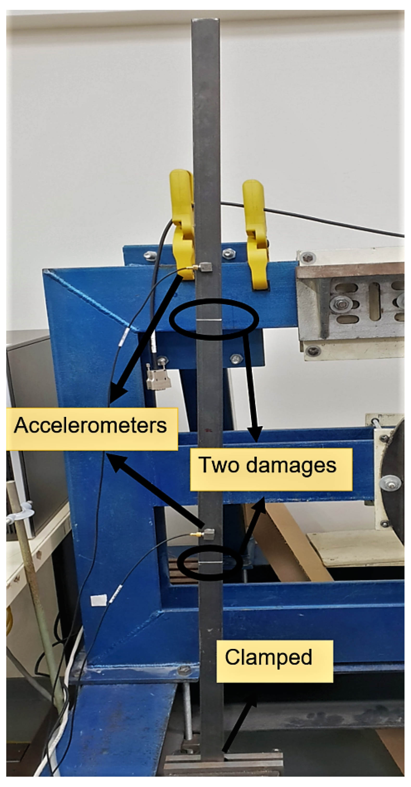
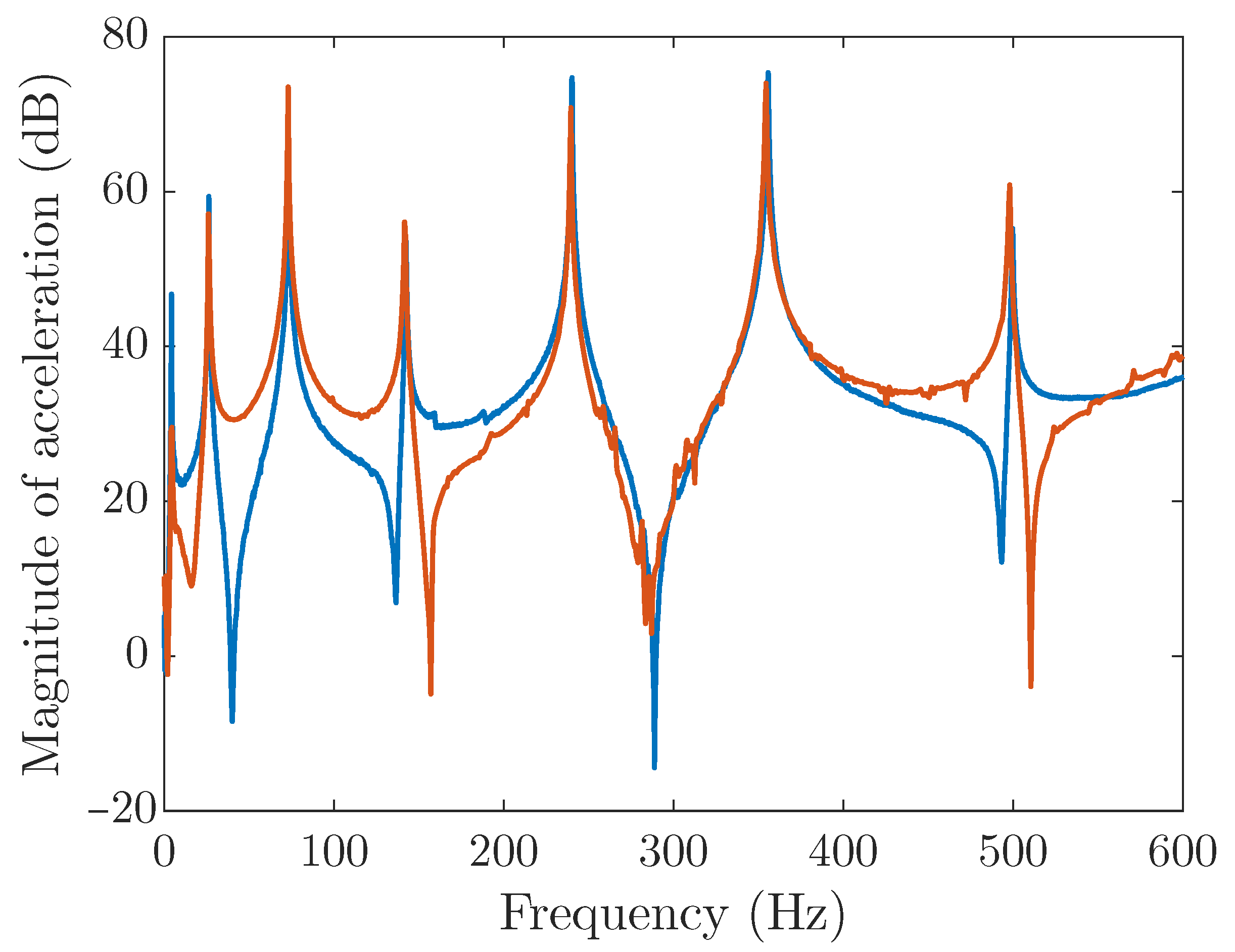
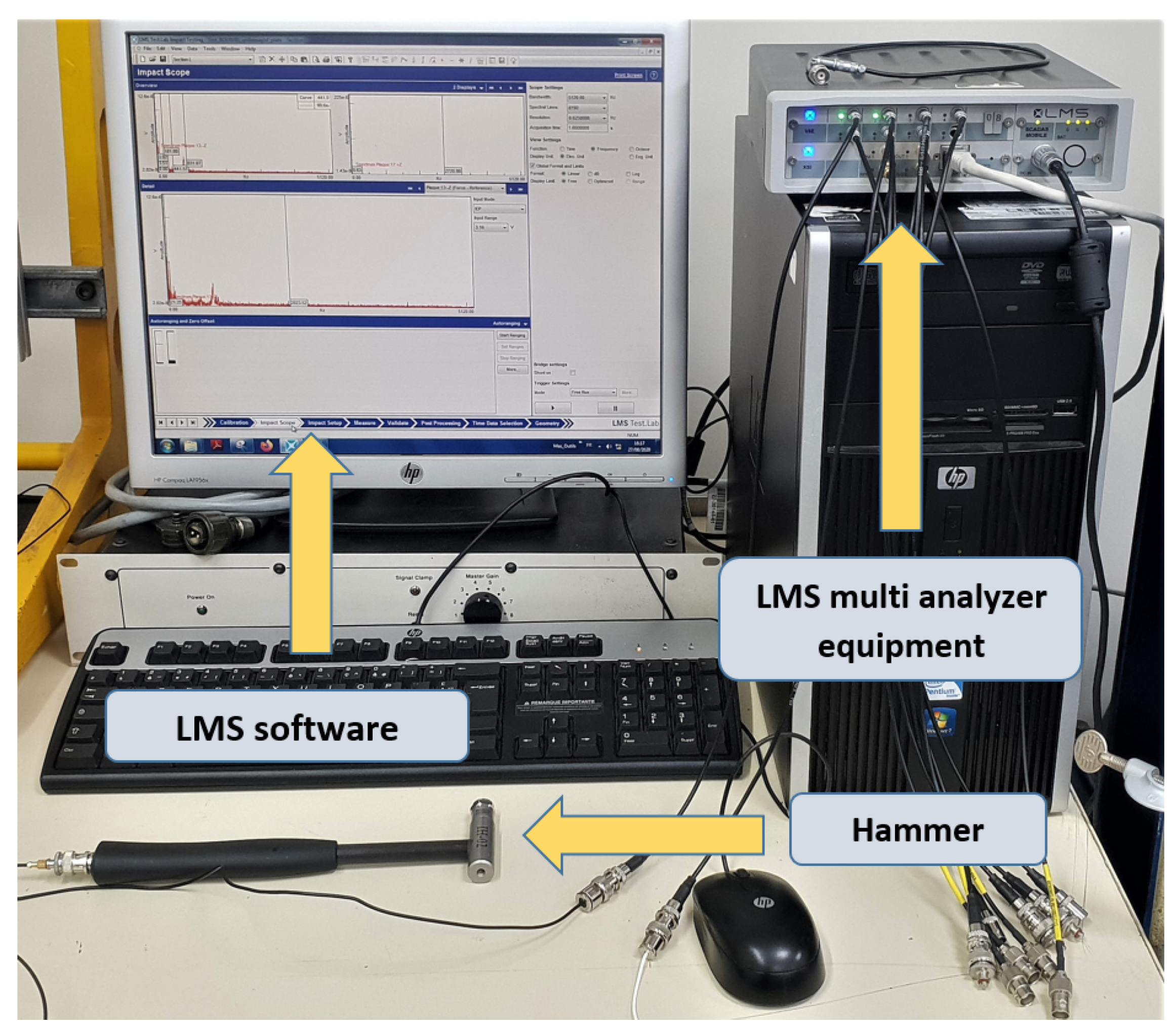
5. Experimental Example for Damage Identification

To estimate positions and severity of the damage in a real structure, a steel beam has been examined with the same material and geometrical properties (see Section 4.1) as those stated in the numerical FE Models. Healthy and damaged beams are used for the experimental test. On the damaged beam, two instances of damage (saw cut) are done. The damage 1 and damage 2 are placed at 0.25 m and 0.68 m beam positions from the clamped end. Damage (damage 1 and damage 2) sizes are also measured. The first (damage 1), was found with a depth of 1.3 mm and a width of 1.15 mm, and the other (damage 2) was obtained with a depth of 1.55 mm and a width of 1.40 mm. In this case, the height of both saw cuts is considered with a similar value of the beam’s height.

During the experimental beam tests, two accelerometers are mounted at different beam positions (0.35 m and 0.75 m). Experimental beam configurations and setup are shown in Figure 10 and Figure 11. A hammer impact test was conducted, and signals with LMS multi-analyzer (Siemens LMS software, Plano, TX, USA) were used to record the vibration measurements. The input excitation was produced by the hammer and output data was recorded by the monoaxial accelerometer (Brüel and Kjær-DeltaTron Type 4507). The beam was clamped on one side with a strong mechanical hinge, while the other side was free. The experimental setup (see Figure 10) was then designed in such a way as to extract natural frequencies from the beams (healthy and damaged). FRFs (see Figure 12) of the healthy and damaged cantilever beam, were used to acquire natural frequencies by implementing the circle fit method with EasyMod Module [47] using MATLAB. 

Table 6. Experimentally identified natural frequencies of healthy and damaged beams.

Experimental Beam	Natural Frequencies (Hz)
	1	2	3	4	5	6	7
$f_{healthy}$	4.27	26.33	73.26	142.34	240.13	355.67	499.66
$f_{damaged}$	4.25	26.22	72.82	141.73	239.38	354.36	497.97

represents the seven experimentally measured natural frequencies of the healthy and damaged real beams.

Results

To classify damage properties (positions and severity), a test is conducted on the basis of the frequency shift between healthy and damaged real beams. The real damaged beam (see Figure 11) is evaluated and compared to the numerical 2D FE healthy and damaged models using FSC. The beam model (see Figure 1) based on the 2D FE mesh (100 elements) is used for the purpose of FSC minimization. As similarly illustrated during double-damaged identification, the representation of Figure 13a,b is done after obtaining the positions and severity using an FSC-based algorithm with particleswarm() solver.

Damages are found at beam positions of 0.244 m and 0.676 m, and severity of these localized damages are estimated with 34.2% and 28.5%, respectively. Here, the error (percentage) for damage positions 1 and 2, are obtained with the values of 2.4% and 0.59%. If we obtain the positions and severity corresponding to the global minimum, then the representation of Figure 13a,b can be performed to indicate the identified damage parameters. Each representation is obtained by considering either positions or severity of respective two damages, which allows FSC to be a function of beam positions and damage severity. Thus, the results indicate that the FSC-based algorithm is well suited for localizing and quantifying damages in the real structure.

6. Conclusions

This work focused on a damage identification algorithm using FE Models and minimization of a frequency shift coefficient. A cantilever beam was investigated throughout this research work. Different damaged cases were localized and quantified using the FSC algorithm. The algorithm was effective at identifying smaller to larger-sized damages, where double damages are located close or far away from each other. In this numerical investigation, the lowest level of severity was estimated at 1%. The numerical outcomes indicate that the proposed algorithm is suitable for identifying single and multiple damages. The sensitivity of the algorithm to uncertainties on natural frequencies was investigated by considering small random perturbations. The results show that perturbed natural frequencies indeed cause small errors in terms of position and severity but that the estimation always falls close to the real damage parameters for small perturbations. The application of natural frequencies, and their feasibility for damage identification based on numerical FE models, was examined. Sensitivity of FSC associated with the algorithm under a variety of damage conditions, as well as an experimental example, was determined. Finally, the experimental results on a beam with two damaged areas corroborate the numerical study and show the efficiency of the algorithm. In the future, the algorithm will be explored with other types of structures, structural behaviors and different boundary conditions in order to validate its efficiency.

References

1. Dai, D.; He, Q. Structure damage localization with ultrasonic guided waves based on a time–frequency method. J. Signal Process. 2014, 96, 21–28. [Google Scholar] [CrossRef]
2. Clarke, T.; Simonetti, F.; Cawley, P. Guided wave health monitoring of complex structures by sparse array systems: Influence of temperature changes on performance. J. Sound Vib. 2010, 329, 2306–2322. [Google Scholar] [CrossRef]
3. Sodano, H.A. Development of an automated eddy current structural health monitoring technique with an extended sensing region for corrosion detection. Struct. Health Monit. 2007, 6, 111–119. [Google Scholar] [CrossRef]
4. Bruno, C.L.E.; Gliozzi, A.S.; Scalerandi, M.; Antonaci, P. Analysis of elastic nonlinearity using the scaling subtraction method. Phys. Rev. B 2009, 79, 064108. [Google Scholar] [CrossRef]
5. Loi, G.; Porcu, M.C.; Aymerich, F. Impact damage detection in composite beams by analysis of non-linearity under pulse excitation. J. Compos. Sci. 2021, 5, 39. [Google Scholar] [CrossRef]
6. Frau, A.; Pieczonka, L.; Porcu, M.C.; Staszewski, W.J.; Aymerich, F. Analysis of elastic nonlinearity for impact damage detection in composite laminates. J. Phys. Conf. Ser. 2015, 628, 012103. [Google Scholar] [CrossRef]
7. Messina, A.; Jones, I.; Williams, E. Damage detection and localization using natural frequency changes. In Proceedings of the Conference on Identification in Engineering Systems, Cambridge, UK, 1 March 1996; pp. 67–76. [Google Scholar]
8. Messina, A.; Williams, E.; Contursi, T. Structural damage detection by a sensitivity and statistical-based method. J. Sound Vib. 1998, 216, 791–808. [Google Scholar] [CrossRef]
9. Pandey, A.; Biswas, M.; Samman, M. Damage detection from changes in curvature mode shapes. J. Sound Vib. 1991, 145, 321–332. [Google Scholar] [CrossRef]
10. Pandey, A.; Biswas, M. Damage detection in structures using changes in flexibility. J. Sound Vib. 1994, 169, 3–17. [Google Scholar] [CrossRef]
11. Doebling, S.W.; Farrar, C.R.; Prime, M.B.; Shevitz, D.W. Damage Identification and Health Monitoring of Structural and Mechanical Systems from Changes in Their Vibration Characteristics: A Literature Review; Technical Report; Los Alamos National Laboratory: Los Alamos, NM, USA, 1996. [Google Scholar] [CrossRef] [Green Version]
12. Rytter, A. Vibrational Based Inspection of Civil Engineering Structures. Ph.D. Thesis, Department of Building Technology and Structural Engineering, Aalborg University, Aalborg, Denmark, 1993. [Google Scholar]
13. Dubey, A.; Denis, V.; Serra, R. A novel VBSHM strategy to identify geometrical damage properties using only frequency changes and damage library. Appl. Sci. 2020, 10, 8717. [Google Scholar] [CrossRef]
14. Huang, M.S.; Gül, M.; Zhu, H.P. Vibration-based structural damage identification under varying temperature effects. J. Aerosp. Eng. 2018, 31, 04018014. [Google Scholar] [CrossRef]
15. Wang, Z.; Huang, M.; Gu, J. Temperature effects on vibration-based damage detection of a reinforced concrete slab. Appl. Sci. 2020, 10, 2869. [Google Scholar] [CrossRef] [Green Version]
16. Toh, G.; Park, J. Review of vibration based structural health monitoring using deep learning. Appl. Sci. 2020, 10, 1680. [Google Scholar] [CrossRef]
17. Salawu, O. Detection of structural damage though changes in frequency: A review. Eng. Struct. 1997, 19, 718–723. [Google Scholar] [CrossRef]
18. Cawley, P.; Adams, R.D. The location of defects in structures from measurements of natural frequencies. J. Strain Anal. Eng. Des. 1979, 14, 49–57. [Google Scholar] [CrossRef]
19. Narkis, Y. Identification of crack location in vibrating simply supported beams. J. Sound Vib. 1994, 172, 549–558. [Google Scholar] [CrossRef]
20. Silva, M.E.; Araujo Gomes, A. Crack identification on simple structural elements through the use of natural frequency variations: The inverse problem. In Proceedings of the 12th International Modal Analysis, Honolulu, HI, USA, 31 January–3 February 1994; pp. 1728–1735. [Google Scholar]
21. Brincker, R.; Andersen, P.; Kirkegaard, P.H.; Ulfkjaer, J. Damage detection in laboratory concrete beams. In Proceedings of the 13th International Modal Analysis Conference, Nashville, TN, USA, 13–16 February 1995; pp. 668–674. [Google Scholar]
22. Kim, J.-T.; Ryu, Y.-S.; Cho, H.-M.; Stubbs, N. Damage identification in beam-type structures: Frequency-based method vs mode-shape-based method. Eng. Struct. 2003, 25, 57–67. [Google Scholar] [CrossRef]
23. Armon, D.; Ben-Haim, Y.; Braun, S. Crack detection in beams by rankordering of eigenfrequency shifts. Mech. Syst. Signal Process. 1994, 8, 81–91. [Google Scholar] [CrossRef]
24. Zhang, Y.; Lie, S.T.; Xiang, Z.; Lu, Q. A frequency shift curve based damage detection method for cylindrical shell structures. J. Sound Vib. 2014, 333, 1671–1683. [Google Scholar] [CrossRef]
25. Gillich, G.R.; Ntakpe, J.L.; Wahab, M.A.; Praisach, Z.I.; Mimis, M.C. Damage detection in multi-span beams based on the analysis of frequency changes. J. Phys. Conf. Ser. 2017, 842, 012033. [Google Scholar] [CrossRef] [Green Version]
26. Shukla, A.; Harsha, S. Vibration response analysis of last stage lp turbine blades for variable size of crack in root. Procedia Technol. 2016, 23, 232–239. [Google Scholar] [CrossRef] [Green Version]
27. Keye, S. Improving the performance of model-based damage detection methods through the use of an updated analytical model. Aerosp. Sci. Technol. 2006, 10, 199–206. [Google Scholar] [CrossRef]
28. Gautier, G.; Mencik, J.M.; Serra, R. A finite element-based subspace fitting approach for structure identification and damage localization. Mech. Syst. Signal Process. 2015, 58, 143–159. [Google Scholar] [CrossRef]
29. Dahak, M.; Touat, N.; Benseddiq, N. On the classification of normalized natural frequencies for damage detection in cantilever beam. J. Sound Vib. 2017, 402, 70–84. [Google Scholar] [CrossRef]
30. Khiem, N.; Toan, L. A novel method for crack detection in beam-like structures by measurements of natural frequencies. J. Sound Vib. 2014, 333, 4084–4103. [Google Scholar] [CrossRef]
31. Le, T.-T.-H.; Point, N.; Argoul, P.; Cumunel, G. Structural changes assessment in axial stressed beams through frequencies variation. Int. J. Mech. Sci. 2016, 110, 41–52. [Google Scholar] [CrossRef]
32. Khatir, S.; Belaidi, I.; Serra, R.; Wahab, M.A.; Khatir, T. Damage detection and localization in composite beam structures based on vibration analysis. Mechanics 2015, 21, 472–479. [Google Scholar] [CrossRef] [Green Version]
33. Yam, L.H.; Li, Y.Y.; Wong, W.O. Sensitivity studies of parameters for damage detection of plate-like structures using static and dynamic approaches. Eng. Struct. 2002, 24, 1465–1475. [Google Scholar] [CrossRef]
34. Serra, R.; Lopez, L.; Gautier, G. Tentative of damage estimation for different damage scenarios on cantilever beam using numerical library. In Proceedings of the 23th International Congress on Sound and Vibration, Athens, Greece, 10–14 July 2016; pp. 10–14. [Google Scholar]
35. Eraky, A.; Anwar, A.M.; Saad, A.; Abdo, A. Damage detection of flexural structural systems using damage index method–experimental approach. Alex. Eng. J. 2015, 54, 497–507. [Google Scholar] [CrossRef]
36. Serra, R.; Lopez, L. Damage detection methodology on beam-like structures based on combined modal wavelet transform strategy. Mech. Ind. 2017, 18, 807. [Google Scholar] [CrossRef] [Green Version]
37. Hu, W.H.; Thöns, S.; Rohrmann, R.G.; Said, S.; Rücker, W. Vibration-based structural health monitoring of a wind turbine system Part II: Environmental/operational effects on dynamic properties. Eng. Struct. 2015, 89, 273–290. [Google Scholar] [CrossRef]
38. Karbhari, V.; Lee, L.S.-W. Vibration-based damage detection techniques for structural health monitoring of civil infrastructure systems. In Struct. Health Monit. Civ. Infrastruct. Syst.; Karbhari, V.M., Ansari, F., Eds.; Woodhead Publishing Limited: Cambridge, UK, 2009; pp. 177–212. [Google Scholar] [CrossRef]
39. Porcu, M.C.; Patteri, D.M.; Melis, S.; Aymerich, F. Effectiveness of the FRF curvature technique for structural health monitoring. Constr. Build. Mater. 2019, 226, 173–187. [Google Scholar] [CrossRef]
40. Furukawa, A.; Kiyono, J. Identification of structural damage based on vibration responses. In Proceedings of the 13th World Conference on Earthquake Engineering, Vancouver, BC, Canada, 1–6 August 2004. [Google Scholar]
41. Mohan, S.; Maiti, D.K.; Maity, D. Structural damage assessment using frequency response function employing particle swarm optimization. Appl. Math. Comput. 2013, 219, 10387–10400. [Google Scholar] [CrossRef]
42. Huang, M.; Lei, Y.; Li, X. Structural damage identification based on l1 regularization and bare bones particle swarm optimization with double jump strategy. Math. Probl. Eng. 2019, 5954104. [Google Scholar] [CrossRef] [Green Version]
43. Li, X.L.; Serra, R.; Olivier, J. Performance of fitness functions based on natural frequencies in defect detection using the standard PSO-FEM approach. Shock Vib. 2021, 8863107. [Google Scholar] [CrossRef]
44. Li, X.L.; Serra, R.; Olivier, J. A multi-component PSO algorithm with leader learning mechanism for structural damage detection. Appl. Soft Comput. 2021, 116, 108315. [Google Scholar] [CrossRef]
45. Alamdari, M.M.; Li, J.; Samali, B. Damage identification using 2-d discrete wavelet transform on extended operational mode shapes. Arch. Civ. Mech. Eng. 2015, 15, 698–710. [Google Scholar] [CrossRef]
46. Kennedy, J.; Eberhart, R. Particle swarm optimization. In Proceedings of the ICNN’95-International Conference on Neural Networks, Perth, Australia, 27 November–1 December 1995; Volume 4, pp. 1942–1948. [Google Scholar]
47. Kouroussis, G.; Fekih, L.B.; Conti, C.; Verlinden, O. Easymod: A matlab/scilab toolbox for teaching modal analysis. In Proceedings of the 19th International Congress on Sound and Vibration, Vilnius, Lithuania, 8–12 July 2012. [Google Scholar]
Figure 1. (a) The 2D FE damaged model of a cantilever beam and (b) cross-section area.
Vibration 05 00003 g001
Figure 2. Flowchart of the proposed strategy for structure damage identification.
Vibration 05 00003 g002
Figure 3. FSC as a function of position and severity (percentage) of the damage. The white circles denote real damage scenarios, where cross symbols and color bar indicate the lowest minimized value (a) 0.15 m with 2%, (b) 0.25 m with 15%, (c) 0.65 m with 8% and (d) 0.80 m with 24%.
Vibration 05 00003 g003
Figure 4. FSC as a function of positions and severity (percentage) where, white circles represent real damaged parameters. Cross symbols and color bars indicate the lowest minimized value. (a) Damage positions are located at 0.24 m and 0.82 m, and (b) the severity of the localized damage is estimated at 3% and 5%, respectively.
Vibration 05 00003 g004
Figure 5. FSC as a function of positions and severity (percentage) where, white circles represent real damaged parameters. Cross symbols and color bars indicate the lowest minimized value. (a) Damage positions are located at 0.60 m and 0.90 m, and (b) the severity of the localized damage is estimated at 30% and 17%, respectively.
Vibration 05 00003 g005
Figure 6. FSC as a function of positions and severity (percentage) where, white circles represent real damaged parameters. Cross symbols and color bars indicate the lowest minimized value. (a) Damage positions are located at 0.34 m and 0.44 m, and (b) the severity of the localized damage is estimated at 9% and 4%, respectively.
Vibration 05 00003 g006
Figure 7. FSC as a function of positions and severity (percentage) where, white circles represent real damaged parameters. Cross symbols and color bars indicate the lowest minimized value. (a) Damage positions are located at 0.10 m and 0.15 m, and (b) the severity of the localized damage is estimated at 60% and 70%, respectively.
Vibration 05 00003 g007
Figure 8. FSC as a function of position and severity (percentage) of the damage. The red plus symbols indicate the position and severity of the artificial damaged case (a) (see Table 5). The white circles (obtained by FE updating strategy using FSC), green cross symbols (obtained by PSO using FSC) indicate the lowest minimized value, where damage positions and severity are identified (a) without perturbation, and (b) 0.1%, (c) 0.2% and (d) 0.3% with perturbation levels.
Vibration 05 00003 g008
Figure 9. FSC as a function of position and severity (percentage), where white circles denote a real identified damaged case. The cross symbols and color bars indicate the lowest minimized value. (a) The damage parameter (position and severity) are estimated at 0.50 m beam position with 0.50% severity, and (b) the red dot denotes the estimated damage parameter without perturbation, while green, (c) yellow and (d) cyan dots denote estimated damage parameters concerning for hundred samples with 0.1%, 0.2% and 0.3% perturbation, respectively.
Vibration 05 00003 g009
Figure 10. Set up of beam hammer impact test using LMS multi-analyzer system (Siemens LMS software).
Vibration 05 00003 g010
Figure 11. Experimental setup of real cantilever damaged beam with accelerometers.
Vibration 05 00003 g011
Figure 12. Frequency response functions (FRFs) curve of the healthy beam (blue curve) and damaged beam (orange curve), at mid position (0.5 m).
Vibration 05 00003 g012
Figure 13. Experimentally tested damaged beam where FSC as a function of position and severity (percentage). The cross symbols and color bars indicate the lowest minimized value. (a) The damage positions are identified at 0.244 m and 0.676 m, and (b) severity of these localized damage are estimated as 34.2% and 28.5%, respectively.
Vibration 05 00003 g013