Article

Nonintrusive Nonlinear Reduced Order Models for Structures in Large Deformations: Validations to Atypical Structures and Basis Construction Aspects

1
SEMTE Faculties of Mechanical and Aerospace Engineering, Arizona State University, Tempe, AZ 85287, USA
2
AFRL/RQHF Structural Sciences Center, Air Force Research Laboratory, Wright Patterson AFB, Dayton, OH 45433, USA
3
Assembly & Test Technology Development, Intel Corp., Chandler, AZ 85226, USA
*
Author to whom correspondence should be addressed.
Vibration 2022, 5(1), 20-58; https://doi.org/10.3390/vibration5010002
Submission received: 20 August 2021 / Revised: 18 December 2021 / Accepted: 4 January 2022 / Published: 15 January 2022
(This article belongs to the Special Issue Model Order Reduction of Nonlinear Systems)

Abstract

:
The focus of this investigation is on reduced order models (ROMs) of the nonlinear geometric response of structures that are built nonintrusively, i.e., from standard outputs of commercial finite element codes. Several structures with atypical loading, boundary conditions, or geometry are considered to not only support the broad applicability of these ROMs but also to exemplify the different steps involved in determining an appropriate basis for the response. This basis is formed here as a combination of linear vibration modes and dual modes, and some of the steps involved follow prior work; others are novel aspects, all of which are covered in significant detail to minimize the expertise needed to develop these ROMs. The comparisons of the static and dynamic responses of these structures predicted by the ROMs and by the underlying finite element models demonstrate the high accuracy that can be achieved with the ROMs, even in the presence of significant nonlinearity.

1. Introduction

Finite element-based linear vibration analyses are commonplace in mechanical and aerospace engineering applications: they are used in early design to meet specifications but also in later phases to understand and correct observed issues; they provide the structural formulation for most aeroelastic analyses, etc. Their ease of use and computational efficiency stems from three key properties of linear structural dynamic models:
(1)
their dynamic response can be expressed in terms of a linear combination of time-independent mode shapes scaled by time varying generalized coordinates. The number of such combinations is, in general (for typical lightly damped structures), very small in comparison to the number of degrees of freedom of the finite element model and does not change if the mesh is refined.
(2)
the governing equations for the generalized coordinates are fixed in form with coefficients that are directly extractable from the finite element model.
(3)
the methodology is applicable regardless of the geometry of the structure, the constitutive relation of its materials (so long as it is linear), the boundary conditions, and the specific loading.
Moreover, such analyses can be performed with any of the standard commercial finite element software and with any/most finite element types.
As is, however, the formulation breaks down if the deformations become large enough that geometric nonlinear effects arise. Unfortunately, for fully clamped thin-walled structures, such effects become noticeable for peak transverse displacements that are rather small, e.g., of the order of only 1/10 of the thickness, and rapidly increase for larger deformations. The alternative to using linear modal methods is full finite element transient analyses, the cost of which grows with the number of degrees of freedom and are much slower in nonlinear geometric conditions than in linear ones. Accordingly, this alternative is not possible at the design level.
Fortunately, reduced order modeling methods developed in the last two decades, e.g., see [1,2,3,4,5,6,7,8,9,10,11,12,13,14,15,16,17,18,19,20,21,22,23,24,25,26,27,28,29,30,31,32,33,34,35] and references therein, provide an extension of the linear modal methods to the nonlinear geometric problem: they effectively meet the three above properties, with some differences, and are also derivable from finite element models built in commercial finite element software. The key differences with the linear approach are, first, that the set of basis functions used to represent the response must include other functions than the standard linear modes, e.g., the dual modes initially introduced in [3], further discussed in [1,4,25], and implemented in [7,8,9,11,21,22,24,33] on different structures, or the more recently devised modal derivatives [23,29]. Second, the governing equations for the generalized coordinates are cubic with respect to these variables, not linear, and, thirdly, the evaluations of the coefficients of these equations is more involved than in the linear case.
The conditions, if any, on the applicability of the methodology are more difficult to assess because the cubic governing equations used have been derived only under specific conditions, i.e., a St. Venant–Kirchhoff material [36], or using the von Karman strain definition [20], both of which should be applicable to at least moderately large deformations. Validations in comparison with full commercial finite element computations (which often use a different nonlinear formulation than those of [20,36]) are thus an important effort in establishing confidence in the broad applicability of these reduced order modeling methods.
Quite naturally, the database of existing validation efforts has focused on fully clamped straight and curved beams, flat plates, and curved shells, which exhibit especially well the classical symptoms of nonlinear geometric problems: membrane stretching, stiffening/softening, snap-throughs, symmetric breaking, etc. Some validations to more complex geometries have also been performed, e.g., a 9-bay stiffened panel [4,7], a segment of a ramp panel [37], a MEMS resonator [29], joined wings [33], an exhaust cover plate [15], and a perforated plate [20]. Regarding boundary conditions, besides fully clamped, cantilevered structures have been considered in the context of a blade [10,11,21], beams [21,27], and several 2D [21] and 3D [22,33] wings. Elastic supports have also been considered connecting the structure to the ground instead of the clamped boundary conditions in context with beams [7,12,30,38] and a blade [10,11,21], and one study included point support [3]. Finally, the loading has often been assumed to be either uniform pressure or concentrated loads, with few studies [7,25,32] considering either a force exciting one particular mode or a non-uniformly distributed load symptomatic of an aerodynamic loading.
In this light, the first focus of this paper is to (i) briefly describe the construction of nonlinear geometric reduced order models (ROMs) and (ii) present detailed numerical validations in comparison with full finite element results for four novel, rather atypical, structural problems to further enrich the above database. The basis for these reduced order models will be obtained as a combination of linear and dual modes. The second part of this paper focuses on providing guidance on the details of the construction of these dual modes (see review in the next section) to enable a non-expert to build them conveniently and efficiently.

2. Nonlinear Reduced Order Modeling: A Focused Methodology Review

The reduced order modeling formulation adopted here represents the displacements of the finite element degrees of freedom stacked in the vector u(t) as
u t = n = 1 N q n t ψ n
where q n t are the time-dependent generalized coordinates and ψ n are the time-invariant basis functions defined in the undeformed configuration. Based on that representation and either assuming a St. Venant-Kirchhoff material [36] or using the von Karman strain definition [20] leads to the following governing equations for the generalized coordinates (summation over repeated indices implied)
M i j q ¨ j t + D i j q ˙ j t + K i j ( 1 )   q j t + K i j l ( 2 ) q j t q l t + K i j l p ( 3 ) q j t q l t q p t = F i t , i = 1 , 2 , N .
In this equation, M i j denotes the elements of the mass matrix, K i j ( 1 ) , K i j l ( 2 ) , and K i j l p ( 3 ) are linear, quadratic, and cubic stiffness coefficients, and F i = ψ i T F is the modal force associated with mode i pulled back to the undeformed configuration as necessary. The damping matrix D i j is added to collectively represent various energy dissipation mechanisms.
The non-intrusive estimation of the stiffness coefficients K i j ( 1 ) , K i j l ( 2 ) , and K i j l p ( 3 ) using a commercial finite element software can be achieved by imposing a series of specific static displacements fields on the structural finite element model, determining for each one either the associated modal forces or the tangent stiffness matrix, and matching this data to what is predicted from the ROM, i.e., from Equation (2). This strategy is particularly efficient if the set of displacement fields are first proportional to each basis function ψ n , then proportional to each pair (and each triplet for the modal force approach) of such functions; see [1,4,39] for details.
The construction of the basis warrants a more detailed discussion. It should first be recognized that the mode shapes used in the linear problem are, in general, not sufficient to accurately describe the nonlinear response. Consider, for example, a clamped-clamped uniform straight beam for which the linear modes are split into two families: those that are purely transverse and the remaining ones that are purely in-plane. Assume next that loading is purely transverse. When this loading is small, e.g., peak displacements of the order of 1% of thickness or less, these displacements are purely transverse and thus can be represented solely using transverse modes. However, for larger loadings, the beam will need to stretch (the “membrane stretching” effect) since the deformed shape is longer than the undeformed one, i.e., the beam will exhibit in-plane deformations that must also be included to account for all deformations.
While the modeling of these in-plane displacements can be achieved using the in-plane modes, this representation requires many of these modes, e.g., see the discussion of [20]. This is due in part to the difference in the natural frequencies of the lowest transverse and in-plane modes, the latter being typically much higher than the former for elongated thin walled structures. The in-plane displacements associated with the membrane stretching exhibit frequencies that are of the same order as the transverse motions that induced them, i.e., typically associated with the low frequency transverse modes, and thus much lower than the in-plane natural frequencies. Thus, these in-plane displacements occur quasi-statically and accordingly without direct connection with the corresponding mode shapes. This situation is significantly worsened for general non-flat structures in which the mode shapes do not split into transverse and in-plane families; a series of high frequency modes would be necessary to model the membrane stretching, but finding which ones is a very challenging problem (see discussion in [1]).
The above discussion demonstrates that the basis functions ψ n will include a set of N t linear modes V i of low natural frequencies, as would be in the linear case, but also N d additional basis functions for capturing the membrane stretching. The functions are selected here as the “dual modes” first introduced in [3] and broadly used thereafter, e.g., see [4,7,8,9,11,21,22,24,25,33,37,38]. Per the above comments, this strategy seeks the high frequency components of the displacements that arise when the structure is forced along the low frequency (typically transverse-dominated) mode shapes V n . Moreover, it is sufficient that this forcing be static since the membrane stretching is a quasi-static deformation. These observations led to the consideration of the static loadings
F n = α n K F E   V n
on the finite element model, where K F E is its linear stiffness matrix and α n are factors to be selected and so are the indices n of the modes. In the linear case, the response w n α n of the structure to the forces of Equation (3) is simply α n   V n . In the nonlinear geometric case, the displacement field is richer and includes contributions from other low frequency modes as well as the desired high frequency components.
It should be noted that this information is, in general, different for different linear modes V n , and thus the analysis below will be repeated for each of these modes leading to a succession of enrichments of the basis, initially comprised of N t linear modes V i and eventually reaching N = N t + N d basis functions ψ n .
To capture the desired high frequency component in the nonlinear response w n α n , it is first projected on all the basis functions ψ n defined at this point, which include the N t selected linear modes and N s < N d dual modes obtained in prior steps. That is,
w n α n = i = 1 N t + N s γ i α n ψ i + U n α n
where γ i α n are the projection coefficients on the current basis and U n α n is a residual orthogonal to all of the current basis functions. Owing to the nonlinearity of the response, this residual does not scale, either linearly or nonlinearly, with α n and thus different values of this factor will give rise to different residuals and different high frequency content. Since the level of response of the structure along the mode V n is unknown in advance, an ensemble of values of α n , denoted as α n , s s = 1, 2, …, m s should be considered that span the expected level of response (see Section 3 and Section 5).
Extracting the next dual mode(s) from the corresponding set of residuals U n , s is achieved by first performing a proper orthogonal decomposition (POD) [40], leading to m s orthogonal eigenvectors φ i ( n ) , which are prime candidates to be the next dual modes to be included in the basis. Practice with these computations has shown that some of these eigenvectors, often those with some of the largest POD eigenvalues, are linear modes of slightly higher frequencies than the N t ones selected and thus are not the desired high frequency components. Accordingly, a sorting of these eigenvectors must be performed that is not simply based on the POD eigenvalues.
This effort is achieved here as in [3] by defining a strain measure associated with each eigenvector. To this end, decompose first the residuals U n , s in its components along the eigenvectors φ j ( n ) as
U n , s = j = 1 m s β s j ( n )   φ j ( n )
where the coefficients β s j ( n ) are
β s j ( n ) = φ j ( n ) T U n , s φ j ( n ) T φ j ( n )
owing to the orthogonality of the POD eigenvectors. Then, the strain measure E i ( n ) for the eigenvector φ i ( n ) is defined as
E i ( n ) = s = 1 m s β s i ( n )   φ i ( n ) T K F E   φ i ( n )
To exhibit a high value of E i ( n ) , a particular eigenvector φ i ( n ) must be significantly present in the residuals U n , s so that the term in parentheses in Equation (7) is large but also must be associated with a large (linear) strain energy φ i ( n ) T K F E   φ i ( n ) , and these are the desired attributes for an eigenvector to be selected as dual mode.
Once the POD eigenvectors have been determined and their strain measures computed and sorted from largest to smallest, it remains to determine how many of these eigenvectors will be selected as dual modes. That number should be such that all novel information on the deflection field present in the residuals U n , s has been extracted.
Two strategies have been used in the past to determine the number of eigenvectors n d that should be selected as duals for a particular linear mode V n in Equation (3). In the first one, all eigenvectors with strain measure larger than a stated fraction ε E of the maximum strain measure are selected. That is, assuming that the POD eigenvectors φ i ( n ) have been renumbered so that their strain measures are decreasing, adopt as duals φ i ( n ) , i = 1, …, n d such that
E n d + 1 ( n ) < ε E   E 1 ( n ) E n d ( n ) E n d 1 ( n ) E 1 ( n )
The second strategy focuses directly on the “representation error” of the residuals U n , s by a tentative set i I of the POD eigenvectors φ i ( n ) . That is,
ε r e p n , s , I = U n , s i I β s i ( n )   φ i ( n ) U n , s
The dual modes are then selected as the set of eigenvectors φ i ( n ) , i I , of minimum size that leads to representation errors ε r e p lower than a specified threshold ε r e p ( t h ) for all load cases s. Note in Equation (9) that the norms are computed for each translation degree of freedom over the entire set of nodes of the finite element model. There are thus 2 representation errors for plane structures (beams) and 3 in general, all of which must be lower than the threshold.
It has been shown [3] that it is not sufficient to consider the duals derived from the loadings of the form of Equation (3) to capture well the membrane stretching. Rather, it is also necessary to consider loadings that are combinations of two different modes, i.e.,
F i j = α i K F E   V i + α j K F E   V j
and, potentially, combinations of three different modes, although this need has never been confirmed in any of the 35 validations considered thus far with a dual modes basis. The need to consider combinations of 2 modes as in Equation (10) arises because the dominant interaction term between transverse dominated modes and the membrane stretching is consistently observed to be the quadratic stiffness terms K i j l ( 2 ) , where i refers to a dual mode but j and l to transverse ones, the same or different ones. Thus, the membrane stretching displacements are, in general, not simply the combinations of effects induced by each linear/transverse mode alone but also include terms related to pairs of these modes. The determination of the duals associated with the combined loading of Equation (10) proceed exactly as above for F n .
In concluding this section, it should be noted that, when the first N t basis ψ n are linear modes V n as stated above—although this is not absolutely required—one has
K F E   V n =   ω n 2   M F E   V n
where M F E is the finite element mass matrix. Then, Equations (3) and (10) can be rewritten as
F n = α ¯ n M F E   V n
and   F i j = α ¯ i M F E   V i + α ¯ j M F E   V j
where α ¯ n =   α n   ω n 2 .

3. Basis Construction: Implementation Details Review

The focus of this section is to discuss specific practical aspects of the general basis construction strategy described in the previous section.

3.1. Selection of the Set of Linear Modes

The linear modes included in the nonlinear ROM basis should include all of the linear modes that would be used in a linear analysis, but additional ones may be necessary to reflect (i) nonlinear coupling between modes, (ii) bifurcations, and (iii) internal resonances. These mechanisms may necessitate the addition of linear modes that were not present in the linear analysis because the associated modal force is zero (for modes within the excitation band), or modes outside of this band. A strategy to estimate nonlinear coupling between modes is discussed in Section 5 and thus provides a means to anticipate the additional linear modes to take to address this mechanism.
Experience with these mechanisms suggests that, if the linear modes are appropriately selected to model them, the predictions of the ROM can nevertheless be accurate, e.g., see [25,41,42] for out of band modes, [7] for modes in band with zero or very small modal force, [5,31,43,44,45] for bifurcations due to mechanical loads, and [27,41,42] for internal resonances.

3.2. Selection of the Modes n in Equations

The nonlinear static problems with loading of the form of Equation (3) are relevant to the response of the structure at the times for which this response is primarily along the mode V n . This observation has thus led to the original suggestion [3] that the modes V n are those that are a “large” component of the response. For Equation (10), a similar discussion suggests that at least one of the two modes V i or V j should be a “large” component of the response.
These arguments are appropriate, but they, unfortunately, are based on properties of the response that are yet unknown. Relying on the linear response to assess the overall magnitudes of the linear modes contributions has generally led to a successful basis except for situations where nonlinear coupling between some linear modes is large, a bifurcation occurs, and/or internal resonance takes place. In those situations, the linear modes that arise/are key in these mechanisms ought to be included among those used for Equations (3) and (10).
An alternate strategy will be described in Section 5.

3.3. Selection of the Values αn

As stated above, an ensemble of values of α n in Equation (3) (or α ¯ n in Equation (11)) should be considered that span the expected level of response because the nonlinearity often expresses itself differently at different deformation levels, although it tends to converge as the deformation becomes large enough. In this light, the maximum values of α n have been taken so that the peak transverse deflection is a multiple (1 to 4 say) of the thickness for fully restrained structures and a fraction (e.g., 10%) of the span for cantilevered ones. This criterion applies for both positive and negative deflections, both sets of which must be represented in the values of α n . Overall, the number of cases ( m s ) considered for each linear mode has usually been taken to be between 10 and 20, which was found to be large enough for the duals to converge. Before carrying out the ensuing analysis of Equations (4)–(7), it is recommended to record the stress induced by the displacements w n α n and to reject any case for which the structure would have failed as such data would be beyond the useful range of the ROM. The failure criterion often leads to a relatively modest maximum value of the peak transverse deflection divided by thickness.
Similar considerations apply to the selection of the values α i and α j of Equation (10) (or α ¯ i and α ¯ j of Equations (12)–(13)), but the relative values of these quantities must be also be discussed. Experience with the dual mode construction suggests that loadings of the form of Equation (10) are important as they exercise the nonlinearity in the presence of two modes, but the relative magnitudes of these modes does not play significantly in the appropriateness of the final basis. Accordingly, the simple choice α i = α j (or α ¯ i = α ¯ j ) has been used consistently.
Section 5 presents additional discussion on the selection of the parameters α n .

3.4. Threshold Values for ε E and ε r e p

The values of ε E in Equation (8) have typically been selected between 0.01 and 0.001, while ε r e p ( t h ) has been taken consistently to be 0.01. The representation error criterion appears to be stricter than the energy measure one (Equation (8)).

4. Validations

The following numerical validations aim at extending the breadth of loading conditions, boundary conditions, and geometries that have been considered in previous ROM publications. They will be carried out by comparing the predicted responses by the ROM and by the full finite element model for typical loadings. In all of them, a Rayleigh damping was assumed with finite element and ROM damping matrices of the form
D F E = α M F E + β K F E
and
D R O M = α M R O M + β K R O M ( 1 )
with equal values of α and β on both. This model was selected because it is convenient to impose on both finite element (in Nastran through DMIG entries or a DMAP alter sequence) and ROM, and, thus, the results of dynamic validations are not subjected to differences in damping.

4.1. Curved Cantilevered Beam

While most structures considered in validations have been restrained on all sides (clamped, simply supported, or on spring support), some cantilevered examples have been investigated, e.g., [10,11,21,22,27,33], in the context of wings and blades. One particular observation drawn from them is that the membrane stretching-transverse deformations coupling is, in general, smaller than it would be if the structure was restrained on all sides. This occurs because the cantilevered structure is more free to stretch and thus exhibits smaller membrane stresses, which affect the transverse behavior. In fact, when the structure is flat, this coupling is so dramatically reduced [21] that the identification of the ROM coefficients following the algorithms of [4,39] can be problematic and that an alternate strategy, specific to flat structures, has been proposed [21].
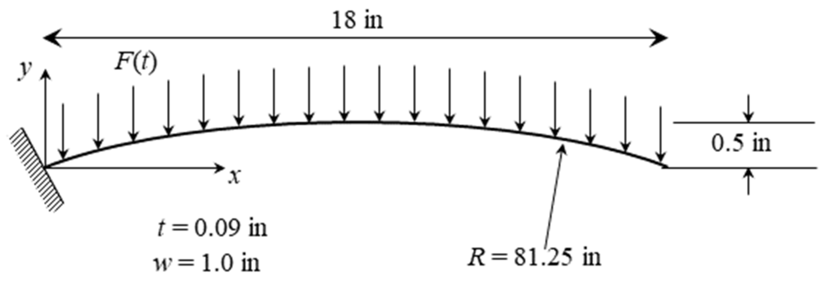
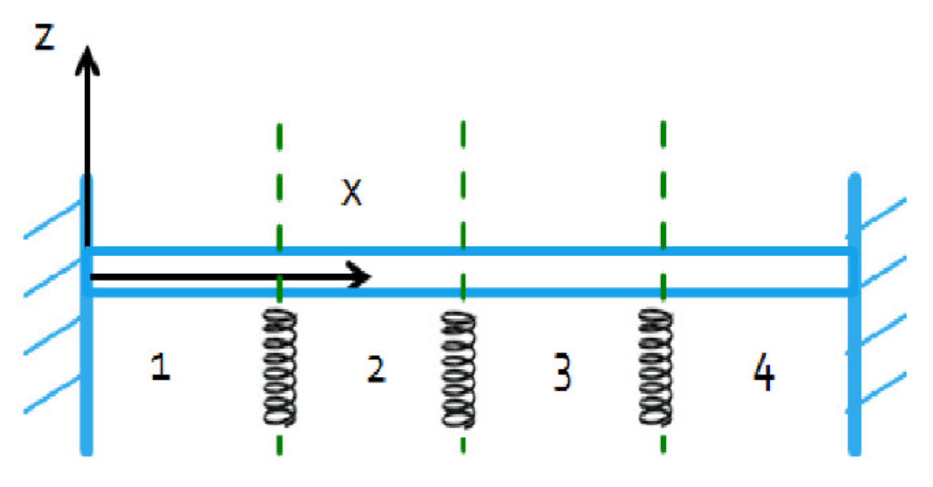
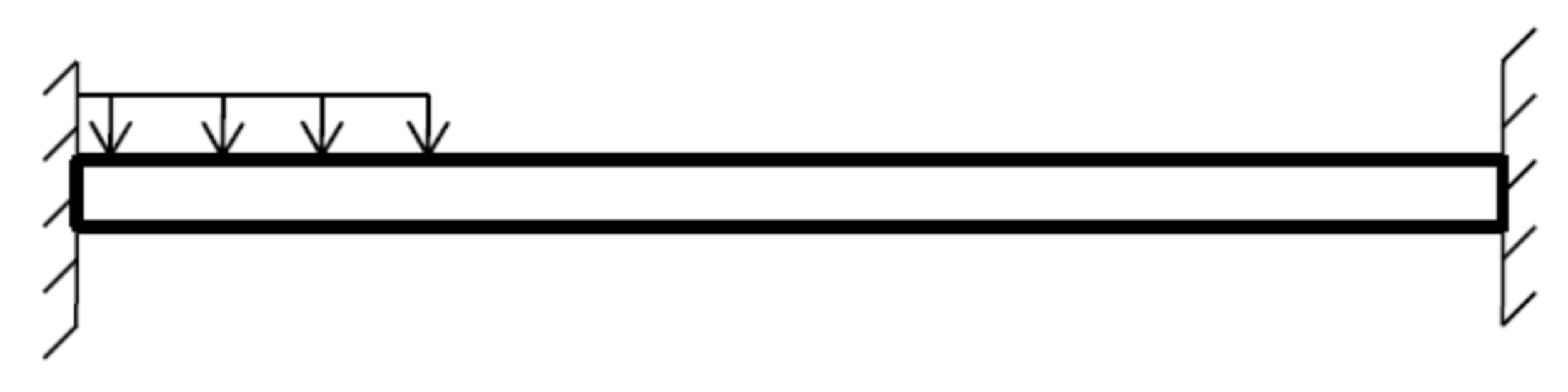
It is desired here to assess whether such issues also occur when the structure is slightly curved. To this end, the curved beam of [5,43] was reconsidered but cantilevered, as shown in Figure 1, as opposed to fully clamped. The material properties were selected as: elastic modulus of 10.6 Mpsi, shear modulus of 4.0 Mpsi, and density of 2.588 × 10⁻⁴ lbf-sec2/in4. The coefficients of the Rayleigh damping were selected as α = 1.0293 1/s and β = 3.8677 × 10⁻⁵ s. The beam was modeled in Nastran using 144 beam elements (CBEAM).
The reduced order model of the beam was constructed under the expectation that it would be subjected to a dynamic loading in the frequency band [0, 100] Hz, and, accordingly, the first 3 linear modes of frequencies 9.05, 56.33, and 83.54 Hz were retained. The fourth mode has natural frequency of 158.24 Hz and thus was not retained as it is significantly above the excitation band cutoff. Given the Rayleigh damping coefficients, the damping ratios of the 3 modes were 1.02%, 0.83%, and 1.11%.
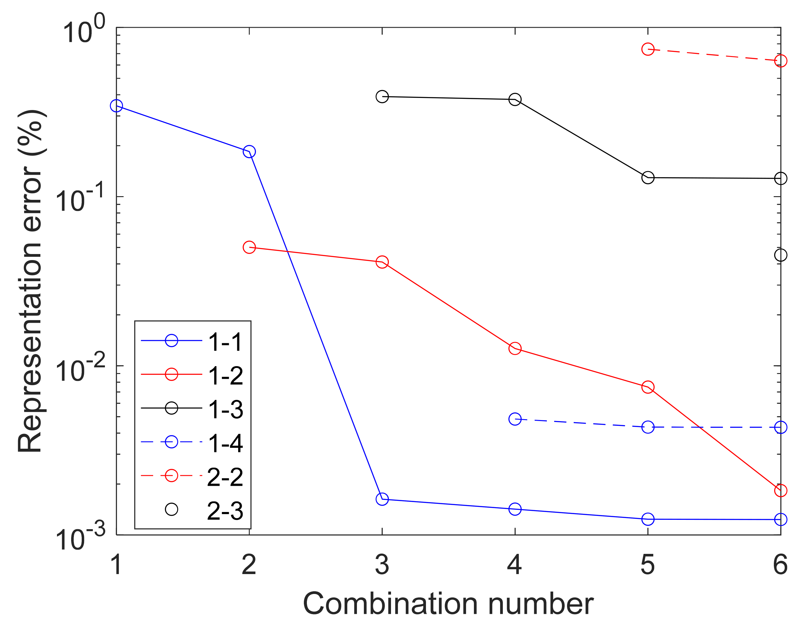
For the determination of the duals, all 6 combinations of the 3 linear modes, i.e., 1-1, 1-2, 1-3, 2-2, 2-3, 3-3, were considered with the data generated as in Equations (12) and (13) with the coefficients α ¯ i = α ¯ j , both positive or negative, spanning the range of induced displacement with peak transverse deflection in the range of 1% to 10% of the span (positive and negative). The representation error criterion of Equation (9) was used to determine the number of duals. The threshold of 1% was achieved by taking a single dual for each combination, see Table 1, leading to a 3L6D basis. The coefficients of the corresponding ROM were then identified according to the tangent stiffness approach of [4].
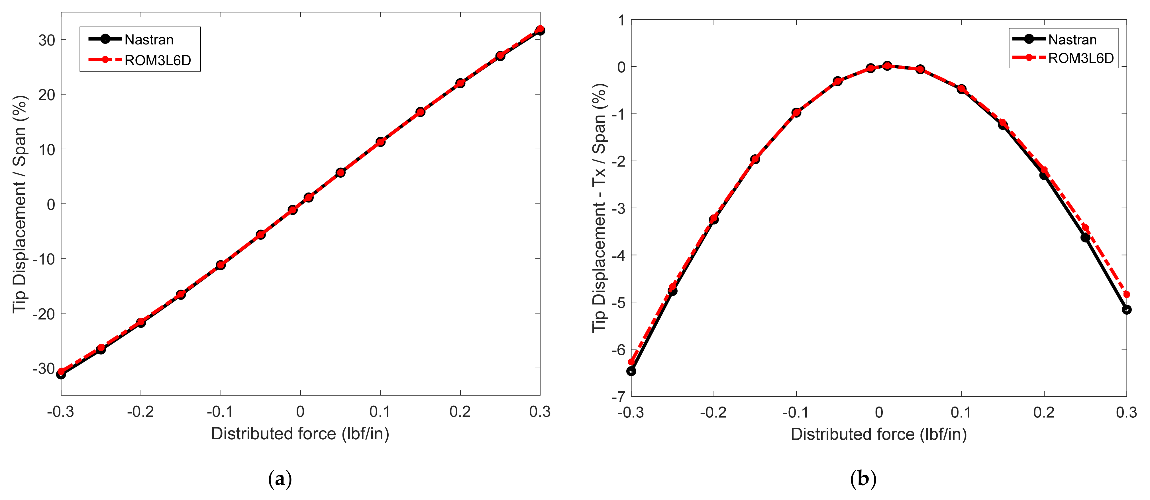
It is often found useful to do a static validation first, and a uniformly distributed load was considered for that effort. The values of the generalized coordinates that would be obtained in the linear case are (with respect to that of mode 1) 1, 1.42 × 10⁻², −3.75 × 10⁻³, and 7.44 × 10⁻⁴. Since the last value is quite small (in relation to that of mode 1), it would appear that the current ROM basis of 3 linear modes is appropriate for this computation. This expectation is confirmed by the results of Figure 2, which shows the transverse (vertical) and in-plane (horizontal) displacements of the beam tip. An excellent matching of the Nastran results is obtained for transverse deflections as large as 30% of the span!
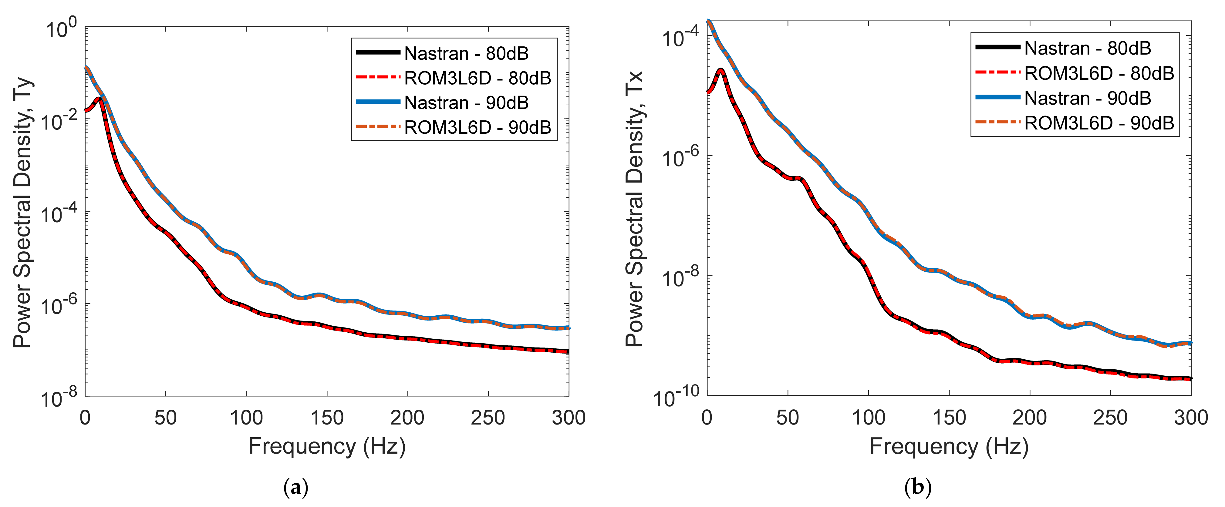
Next, a dynamic validation was performed using a uniformly distributed pressure varying as a bandlimited white noise in the frequency range [0, 100] Hz. Shown in Figure 3 are comparisons of the Nastran and ROM predicted power spectral densities of the transverse and in-plane tip deflections corresponding to 80dB and 90dB excitations, which give rise to standard deviations of tip transverse deflections of 4.15% and 7.73 of span or 8.30 and 15.46 thicknesses, respectively. Again, an excellent agreement is obtained.

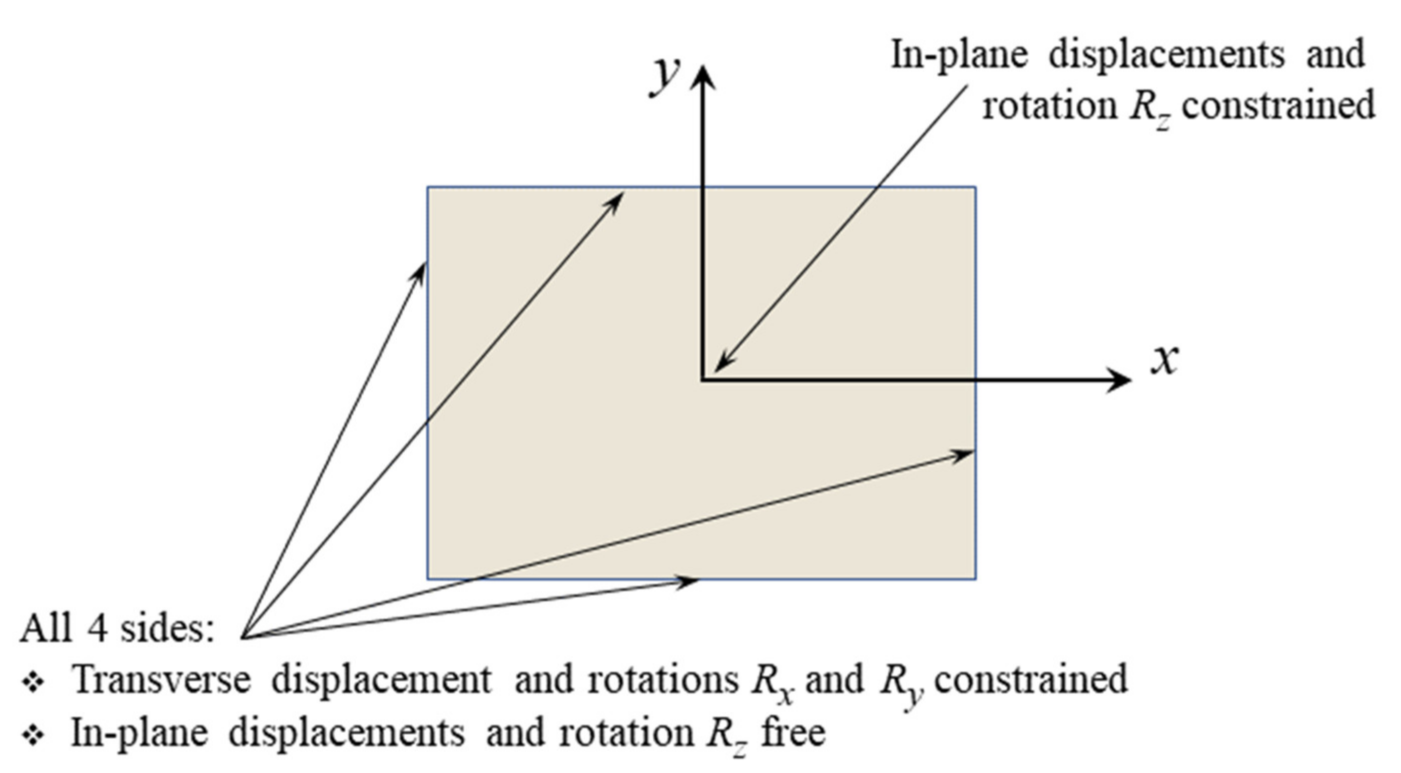
4.2. Freely Expanding Plate

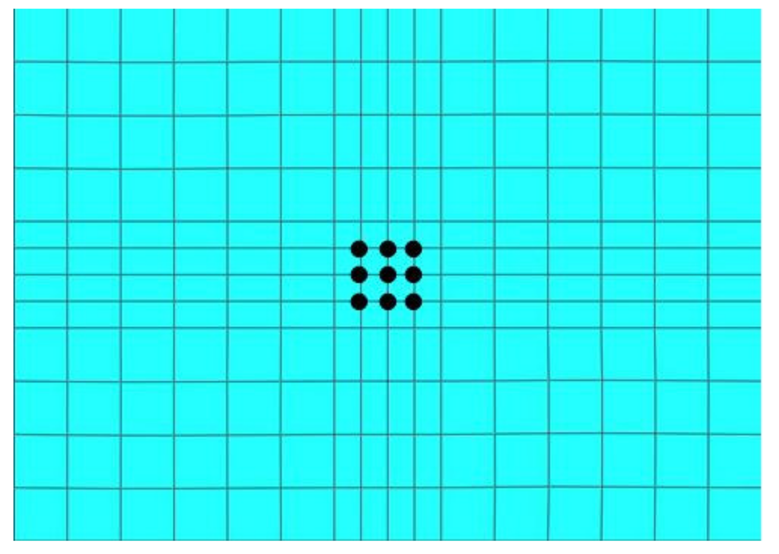
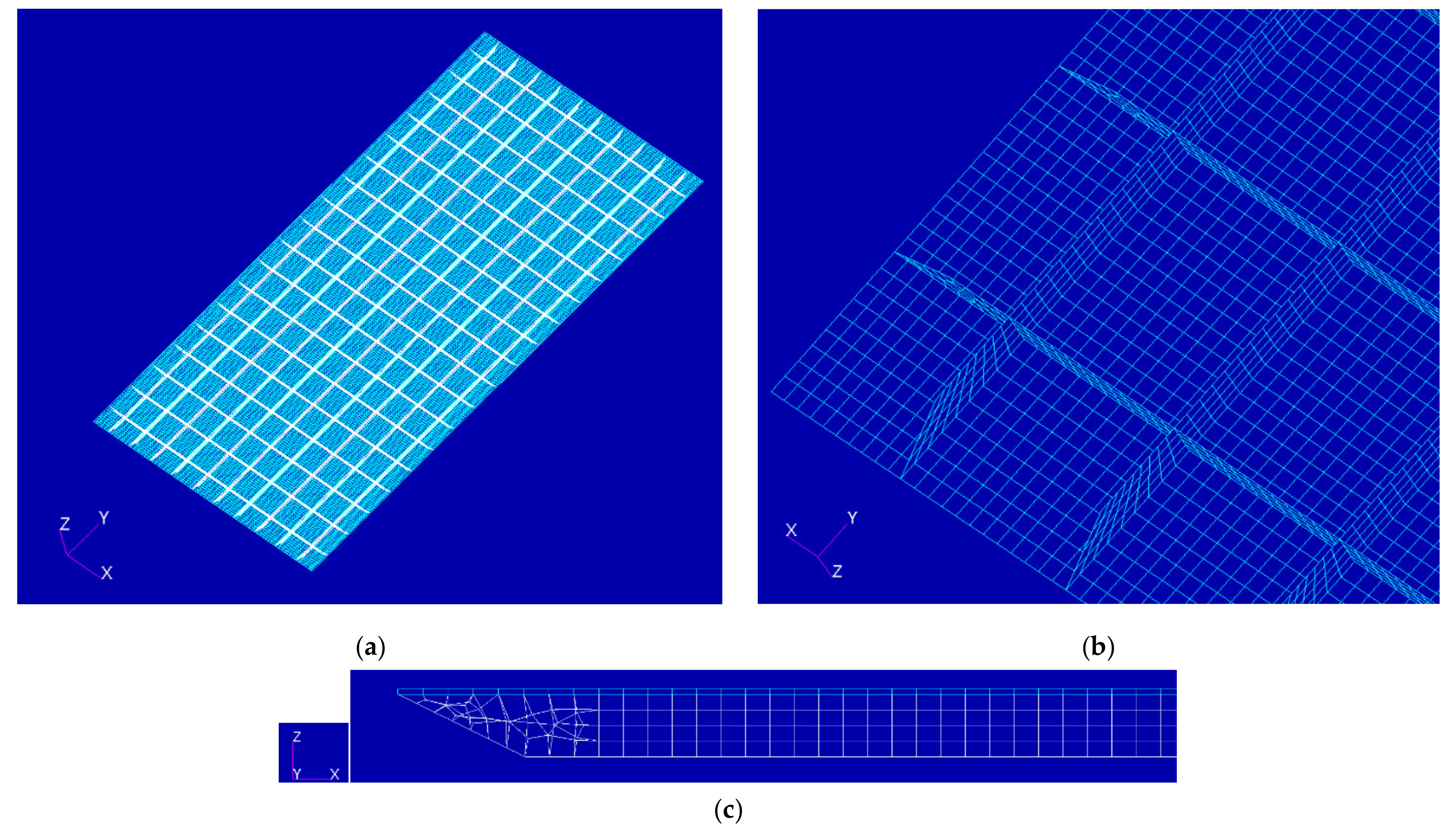
The next validation focuses on an atypical boundary condition that could be considered between cantilevered and clamped. Specifically, the transverse displacement and rotation will be constrained (as if being clamped), while in-plane displacements will be allowed (as would be if cantilevered). A flat plate model is considered with this “freely expanding” boundary condition (see Figure 4). Note that the in-plane displacements and the transverse rotation are fixed at the plate middle to prevent the occurrence of rigid body modes. In the finite element implementation, this single point boundary condition was actually extended over a 3 × 3 array of nodes at the center of the plate (see Figure 5). The freely expanding boundary condition is useful for structures that are heated as the thermally induced expansion is free to occur, thereby preventing the risk of thermal buckling, and has apparently been used on the SR-71.
The geometrical and material properties of this panel are given in Table 2. It was discretized in Nastran using 16 × 12 4-node shell elements (CQUAD4), as shown in Figure 5. The coefficients of the Rayleigh damping were selected as α = 12.838/s and β = 2.061 × 10⁻⁶ s.
It was desired to construct a ROM in anticipation of a uniform (or doubly symmetric) pressure distribution varying in time as a bandlimited white noise in the range of [0, 1040] Hz, and the modes retained had that property. The natural frequencies (in Hz) and corresponding damping ratios (in parentheses) of the first doubly symmetric modes were found to be 110 (1.00%), 300 (0.53%), 525 (0.53%), 700 (0.60%), 704 (0.60%), and 1090 (0.80%).
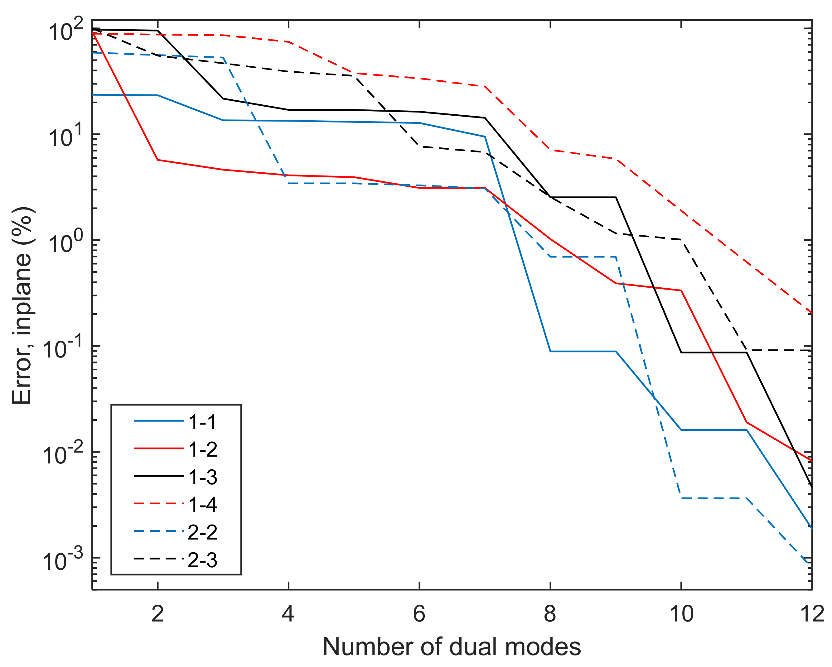
The ROM was constructed using the 6 modes above (all effectively in band). Mode 1 was expected to be the significantly dominant mode, and, thus, the combinations considered for the dual modes were 1-1, 1-2, 1-3, 1-4, 1-5, 1-6. In addition, the 2-2 combination was also added, recognizing that mode 2 also has a notable contribution to the response. The peak transverse displacements were selected to be 1.6 thickness. Selecting one eigenvector as dual for each combination led to 7 duals and a 13-mode basis. The representation errors of the data generated to create the duals by the 13 modes are well below the 1% threshold, e.g., see Table 3. Accordingly, the 6L7D ROM basis was retained and the corresponding stiffness coefficients were identified using the modal force approach of [39].
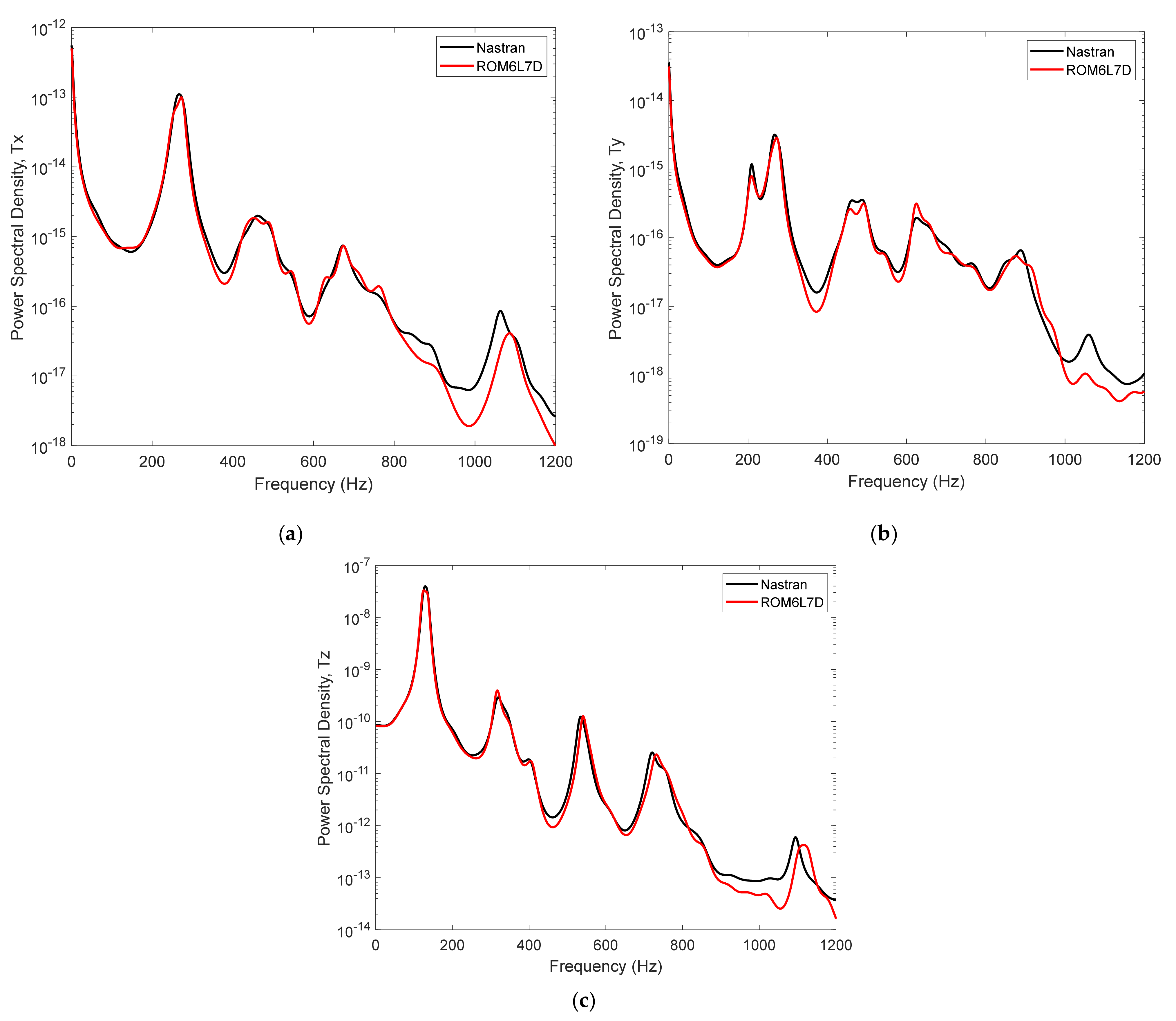
The produced ROM performed very well in comparison with the full finite element model. As an example, note the accurate matching of the power spectral densities of the transverse response of the panel middle and the in-plane displacements of a corner obtained with the ROM and the full finite element model shown in Figure 6. The excitation sound pressure level is 147 dB, leading to standard deviations of the peak transverse displacement of 1.2 thickness and in-plane displacements of the corners of 0.004 and 0.0008 thicknesses in the x and y directions, respectively.
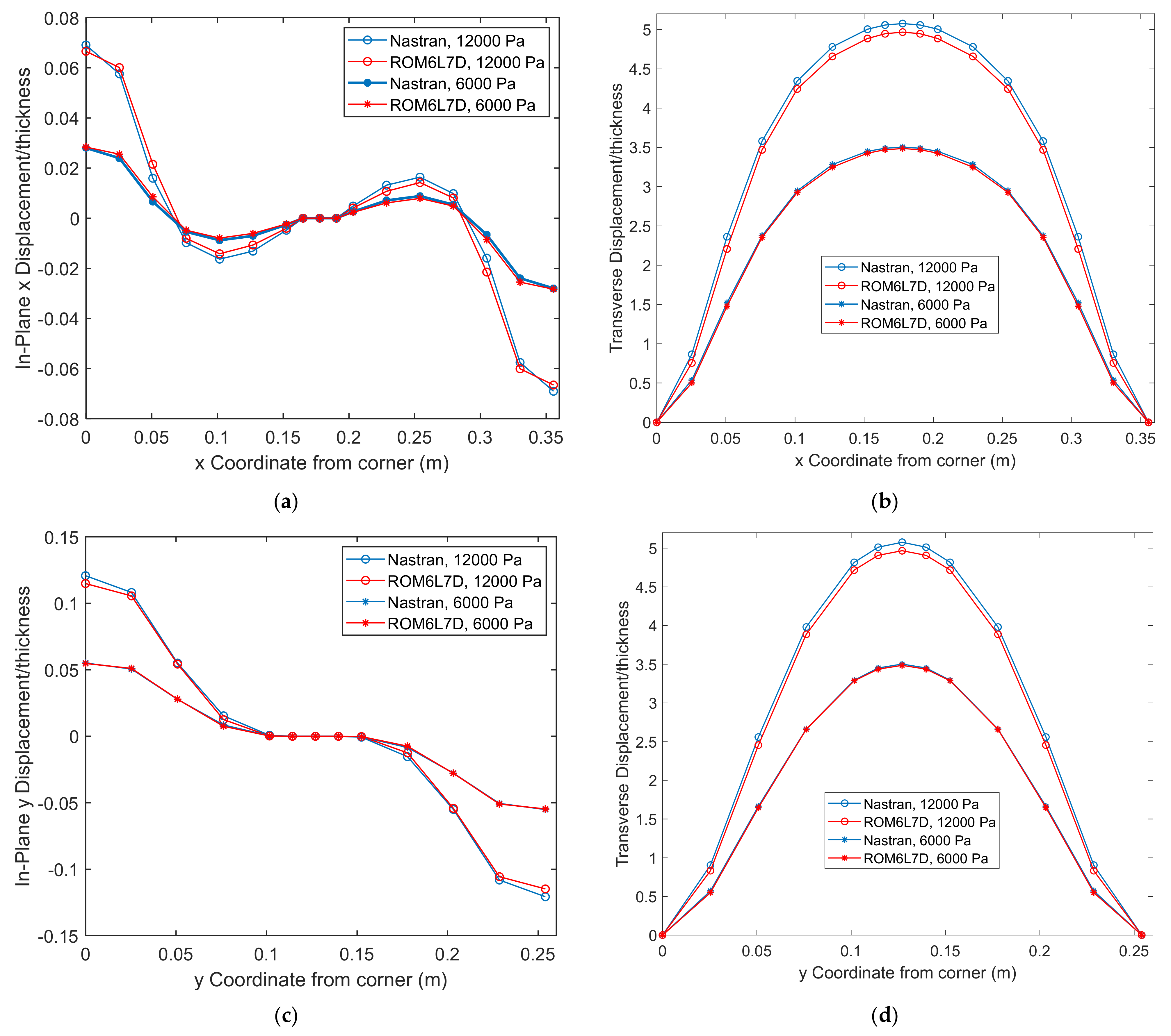
It was also of interest to check the applicability of the ROM to a similar but static loading, and a uniform load was chosen for that purpose. Shown in Figure 7 are the nonzero displacements along the middle lines y = 0 and x = 0 for the two different pressures of 6000 Pa and 12,000 Pa, leading to large nonlinear deflections, i.e., peak transverse deflections of 3.5 and 5.1 thicknesses. At the lowest, still high, level, the matching between the 6L7D ROM and finite element model predictions is nearly perfect. At the very high level of 5.1 thickness, the ROM underestimates the peak response by only 2%, a very good prediction. Note in Figure 7a,c the zero in-plane displacements at the nodes with black dots in Figure 5.
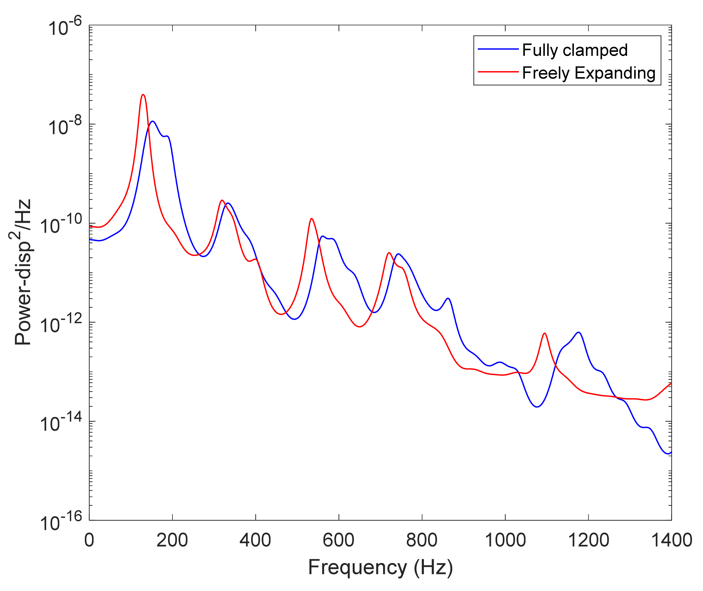
It is interesting to compare the response of this panel to its fully clamped counterpart; see Figure 8 for the transverse displacements of the panel center. The unconstrained in-plane displacements have effectively reduced the nonlinearity of the panel in the transverse direction, as is seen by (i) the increase in peak response in modes 1, 3, and 6, (ii) the reduced shift of the peaks of the spectrum as compared to the natural frequencies, and (iii) the smaller width of these peaks.
The reduced nonlinearity can also be drawn from the ROM coefficients. For flat structures, one can differentiate two sets of cubic nonlinear terms for the linear modes (see [21]). One set of coefficients corresponds to the in-plane displacements fixed; these are the coefficients of the ROM as the linear modes are purely transverse and the duals purely in-plane. Then, when imposing displacement fields along the linear modes to get the coefficients K i j l p ( 3 ) (see [4,39]) with all indices relating to linear modes, no in-plane motion occurs. The other set of coefficients, referred to as condensed and denoted K ^ i j l p ( 3 ) , correspond to the transverse nonlinearity observed when the in-plane displacements occur as needed. These coefficients can either be derived from the ROM through a static condensation of the in-plane/dual generalized coordinates or by an appropriate finite element computation (see [21] for details).
The difference between the corresponding ROM coefficients of the two sets quantifies the softening induced by the membrane stretching/in-plane displacements. Since mode 1 is dominant in both responses, it is sufficient here to consider the coefficients K 1111 ( 3 ) and K ^ 1111 ( 3 ) (see Table 4). For the freely expanding plate, it is seen that K ^ 1111 ( 3 ) is 17% of K 1111 ( 3 ) , i.e., the in-plane displacements reduce the nonlinear stiffening by 83%. For the sake of comparison, for the identical but fully clamped plate, this reduction is only 31% (see Table 4). Moreover, for flat cantilevered structures, this reduction is by factors of the order of 99% with the ratio K ^ 1111 ( 3 ) / K 1111 ( 3 ) of the order of 10−4 or less (see [21]). Thus, as stated above, the freely expanding boundary condition appears as an intermediate between fully clamped and cantilevered.
Analyzing the coefficients of Table 4, it should be noted that the transverse–in-plane coupling coefficient K 117 ( 2 ) is actually smaller for the freely expanding plate than for the fully clamped one, but it is the much reduced value of the in-plane natural frequency (i.e., K 77 ( 1 ) ) that triggers the higher membrane stretching effect. It implies larger in-plane displacements in comparison to the fully clamped plate, which induce the larger softening of the transverse nonlinearity even though the coupling terms are smaller.

4.3. Orthogrid Panel

The advantages of using finite element models developed in commercial software and then reducing them to ROMs are most impactful on complex structures. This was, in particular, demonstrated on the 9-bay panels of [4,7], but another interesting example is the orthogrid panel created by Boeing [46] and subsequently considered in [47]. The finite element model developed in [47] is shown in Figure 9 and its geometry and material properties are summarized in Table 5. It consists of a flat rectangular skin stiffened on its underside by an 18 × 10 array of stiffeners tapered at the edges and of identical material as the skin. It was modeled within Nastran using 48,400 4-node shell elements (CQUAD4) and approximately the same number of nodes for about 290,000 degrees of freedom (see discussion in [47]).
This panel was introduced in [46,47] for coupled aerodynamic–thermal–structural analyses in which the structural deformations were considered quasi-statically. Accordingly, the focus here is on the development of a ROM for static nonlinear analyses, so the selection of the linear modes based on the frequency band of the excitation is not relevant. This observation is clearly true not only for the nonlinear ROM but also for a linear modal model. Following the above recommendations (Section 3), the linear modes to be used for the linear problem will thus first be clarified, and this analysis will be achieved using uncertainty propagation concepts.
Specifically, it is known that small variations in geometry and material properties, collectively referred to as “structural uncertainty”, affect the response of structures, especially in zones of high modal density, which are prone to occur at “high” frequencies. Thus, above a certain frequency band, the deterministic finite element solution is, in general, not an accurate representation of the response of nominally identical but actually different structures because the variability between them induces “large” random variations to the response. The validity of the deterministic reduced order model to be developed thus does not need to extend into that “high frequency” domain since there is no accurate deterministic baseline model available. Effectively, this criterion provides an upper limit to the number of modes to be considered.
This discussion is particularly relevant for the orthogrid panel of Figure 9, which is composed of nominally identical cells connected to each other. It can thus be viewed as a two-dimensional chain, and structures of this type are known to potentially exhibit localization of the free response and high sensitivity of the forced response to small variations of the properties of the chain elements.
The uncertainty propagation analysis was carried out on the linear structural problem by adopting the nonparametric maximum entropy (MaxEnt) approach of [48,49] (see also [36]) and assuming that the uncertainty is in the stiffness properties (since the desired model is to be used for static analyses). This approach assumes that a (linear) ROM of the structure has first been established and its stiffness matrix is denoted as K L . This matrix is then replaced by a random one K ˜ L , which is expressed as
K ˜ L = L   H K   H K T   L T
where L is any decomposition, e.g., Cholesky for simplicity, of K L as
K L = L   L T .
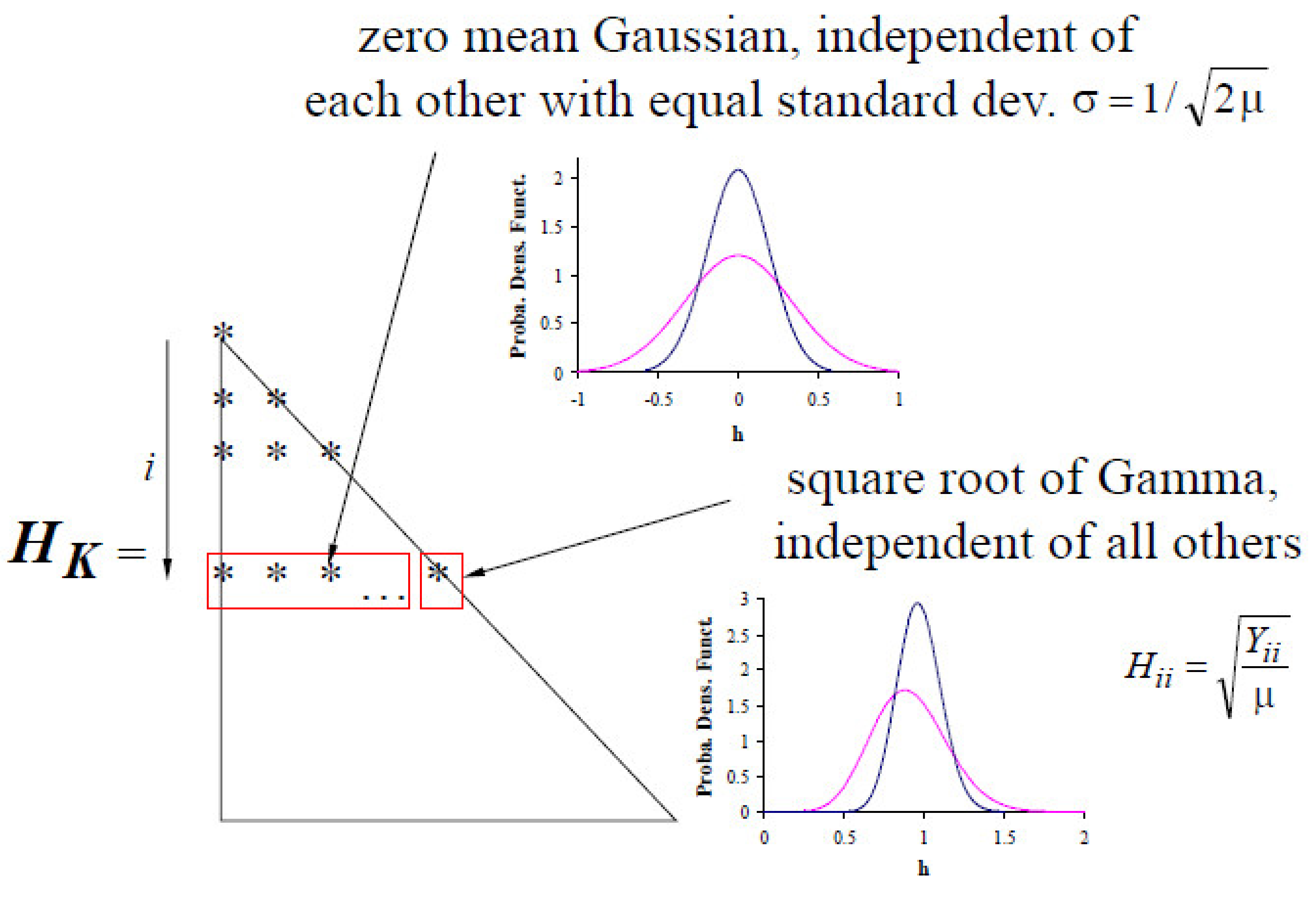
Moreover, in Equation (16), the random matrix H K , see Figure 10, is lower triangular, with all of its elements independent of each other and the off diagonal ones identically distributed as zero mean Gaussian random variables with common standard deviation σ. Finally, the diagonal elements of H K can be expressed as H k k = Y k / μ , where Y k is a Gamma random variable of parameter p k . In these definitions, one has
σ = 1 / 2 μ ;
μ = n + 1 2 δ 2
and   p k = 2 μ k
where n is the size of the matrix K L   and δ represents the overall level of randomness, defined as the coefficient of variation of the random matrix H K H K T .
The first 200 linear, mass normalized modes of the orthogrid panel were selected as basis for the above linear ROM. Accordingly, the matrix K L   was 200 × 200, diagonal with elements equal to the squared natural frequencies. Accordingly, L, see Equation (17), was also diagonal with elements equal to the frequencies. Then, 50 samples of the full random matrix K ˜ L   were simulated as above with δ = 0.1, which induces coefficients of variations (ratio of standard deviation by mean) of the 200 natural frequencies in the range of 0.4% to 0.6% for the frequency up to about 1300 Hz and drops to the range of 0.1% to 0.2% afterwards.
To assess the impact of the uncertainty on the linear forced response of the panel, the transfer functions of the response at various points were computed for each sample of stiffness matrix K ˜ L   assuming a uniformly distributed pressure on the skin varying harmonically in time. A Rayleigh damping was selected for these computations with α = 13.95/s and β = 2.386 × 10
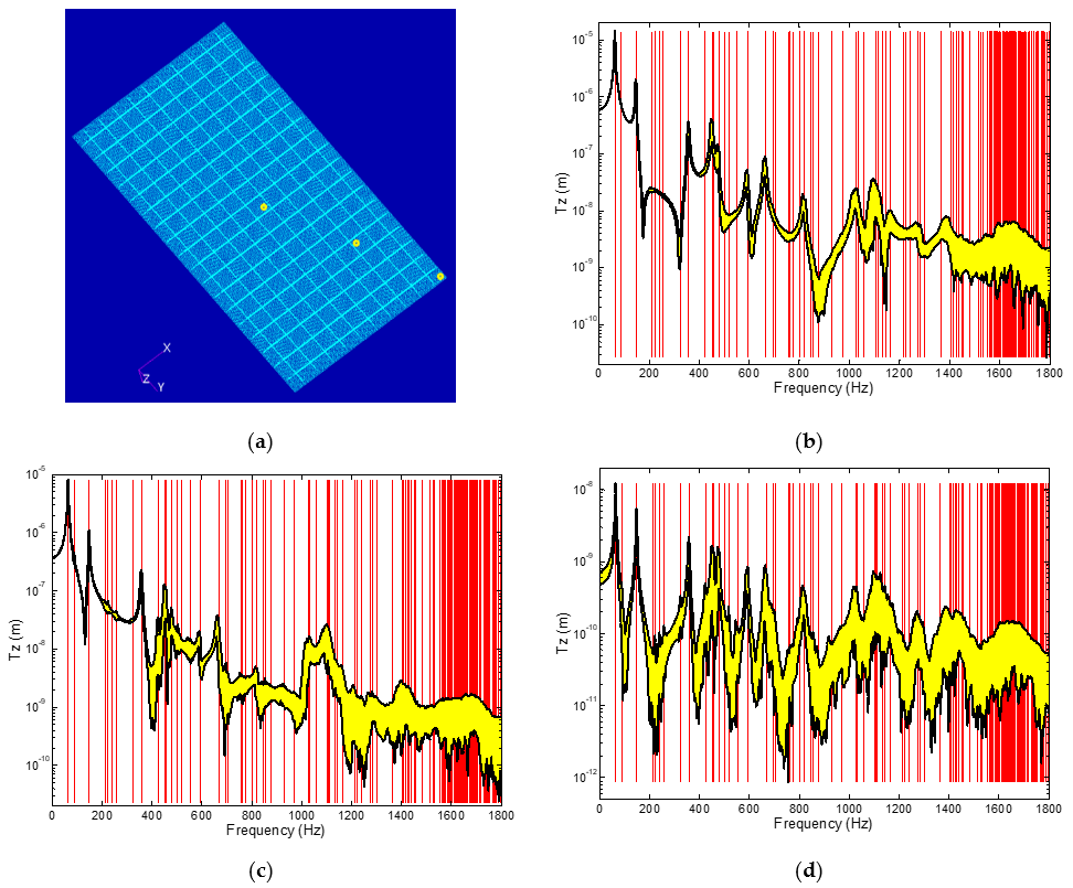
⁻⁶ s, which leads to damping ratios from 0.5% to 2% for the modes in the current frequency range. Shown in Figure 11 are typical results of these computations for the three locations of the panel shown in Figure 11a, i.e., the center point, a quarter point, and a point close to the edge. The figures of Figure 11b–d display (in yellow) the uncertainty bands of the transfer functions corresponding to the range between the 5th and the 95th percentiles of the responses and thus include 90% of the responses. Note on these figures that the red lines indicate the natural frequencies of the deterministic panel, which clearly become densely populated at high frequencies.
It is observed in Figure 11b–d that the uncertainty bands are narrow at low frequencies when the natural frequencies are well separated but become much more wide where the modal density is increasing. In these zones, the peaks also become broader due to the interactions of the modes of varying (random) natural frequencies and mode shapes. In these zones, i.e., for frequencies higher than 1100 Hz or so, the deterministic ROM would provide only one estimate of the response vs. the wide range of responses that can be expected from a physical panel. Accordingly, such a deterministic ROM should not be used above 1100 Hz as it would not be accurate. This frequency is thus set as the upper bound on the frequency range of interest. In this range, there are 33 linear modes of the panel, which will all be included in the nonlinear ROM basis.
For the construction of the duals, the first 4 symmetric modes (Modes 1, 3, 9, and 11) and the first 4 asymmetric modes (Modes 2, 4, 5, and 6) were selected to generate the required load cases (see Equations (3) and (10)). More specifically, the following 26 combinations of modes were considered: 1-1, 1-2, 1-3, 1-4, 1-5, 1-6, 1-9, 1-11, 2-2, 2-3, 2-4, 2-5, 2-6, 2-9, 2-11, 3-3, 3-4, 3-5, 3-6, 3-9, 3-11, 4-4, 4-5, 4-6, 4-9, and 4-11. For each combination, a set of 14 load factors were used to generate 14 force loadings of various magnitudes such that the maximum transverse displacement varies from 0.01 h to 4.0 h, where h is the thickness of the panel skin.
The usual procedure from that point on is to adopt all linear modes, then add on the dual modes one at a time from the residuals of the projections on all linear modes and prior duals of the 14 nonlinear static responses corresponding to each combination of linear modes considered. In this process, the first dual, i.e., the one associated with the dominant linear mode, is not coupled to just this mode but to all linear modes to which it was made orthogonal to by construction of the residuals. This property implies a broader coupling between duals and all linear modes than is physically expected, which, unfortunately, has been observed to be detrimental to the numerical stability of constructed ROMs with a large number of basis functions—as is the case for this panel. This issue is purely numerical and results from small inaccuracies in the identification of the large number of ROM coefficients.
A better approach proposed here is to construct first a “core reduced order model”, i.e., a ROM with only a few modes (linear and duals), that captures qualitatively the behavior of the panel but does not quite have the accuracy desired. This core ROM is then extended by adding sequentially linear modes and their associated duals as necessary. This process narrows the coupling between modes and has been found to enhance the identified ROM numerical stability.
For the current panel model, a core ROM including the 8 linear modes 1-6, 9, and 11 and 9 associated duals (i.e., ROM8L9D) resulting from the combinations of the basis functions 1-1, 1-3, 1-5, 2-4, 3-4, 3-5, 4-4, 2-8, 3-7 (1 dual each) was selected. The construction of the full ROM was then achieved by adding the linear modes 9-33 and, as necessary, their duals. The steps were specifically:
  • given the available core basis (8L9D), the remaining linear modes in the frequency range [0, 1100] Hz were first added to the core basis, yielding a 33L9D basis;
  • the residues of the nonlinear static response data corresponding to linear combinations of linear modes not involved in the core ROM dual modes were computed by making them orthogonal to the basis 33L9D;
  • the duals from the POD eigenvectors of these residues were selected and added to the 33L9D basis to obtain the modified full basis.
For the current panel model, the selection of duals gave rise to a full basis of 33 linear modes and 25 duals. The tangent stiffness matrix procedure was then used to identify the nonlinear stiffness coefficients of this full ROM (33L25D), as well as the core one (8L9D).
The representation errors of the data corresponding to the 26 linear combinations of Equations (3) and (10) are shown in Table 6 for both 8L9D and 33L25D bases. Note in this table that the combinations with a * were used for the construction of the 9 duals of the core 8L9D model. For most of the combinations, the errors obtained with the 33L25D are below or about the typical threshold of 1% in all 3 directions, suggesting that this basis should be appropriate.
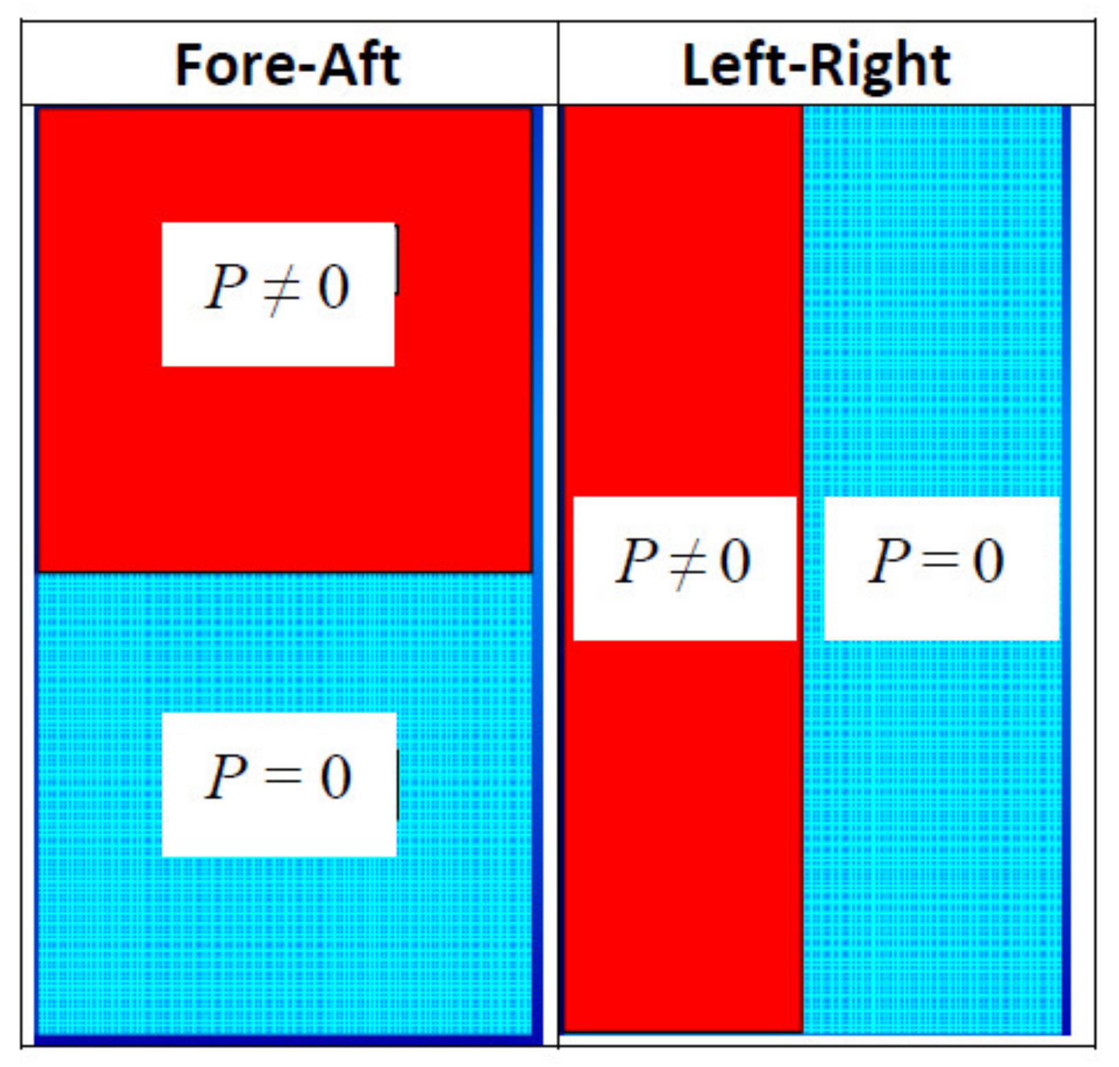
Nonlinear static validations were carried out for both the core (8L9D) and full (33L25D) ROMs by comparing several nonlinear static responses obtained from Nastran and their counterparts predicted by the ROMs. Three static pressure loadings of varying magnitude were considered for this effort: (1) a uniform pressure; (2) a pressure distribution asymmetric in the y-direction (fore-aft) but symmetric in the x-direction (left-right); and (3) a pressure distribution symmetric in the y-direction (fore-aft) but asymmetric in the x-direction (left-right). The last 2 pressure distributions are depicted in Figure 12. All pressures were applied only to the top surface of the panel skin.
For the uniform pressure loading, the pressure was varied from −20 kPa to +20 kPa, with negative pressures applied toward the top surface. The maximum transverse displacements computed by Nastran are about five and six thicknesses, for the negative and the positive pressures, respectively.
Shown in Figure 13 is the resulting comparison of the displacements obtained by Nastran and the two ROMs, at the center and a quarter point of the panel skin. Both ROMs predict transverse displacements very well, at both the center and the quarter point, with the full ROM slightly closer to Nastran. The predictions of in-plane displacements by the two ROMs also agree well to Nastran results. Note that the in-plane displacements of the center point are very small owing to the symmetry of the panel, and, thus, the comparison there is not particularly worthwhile. 
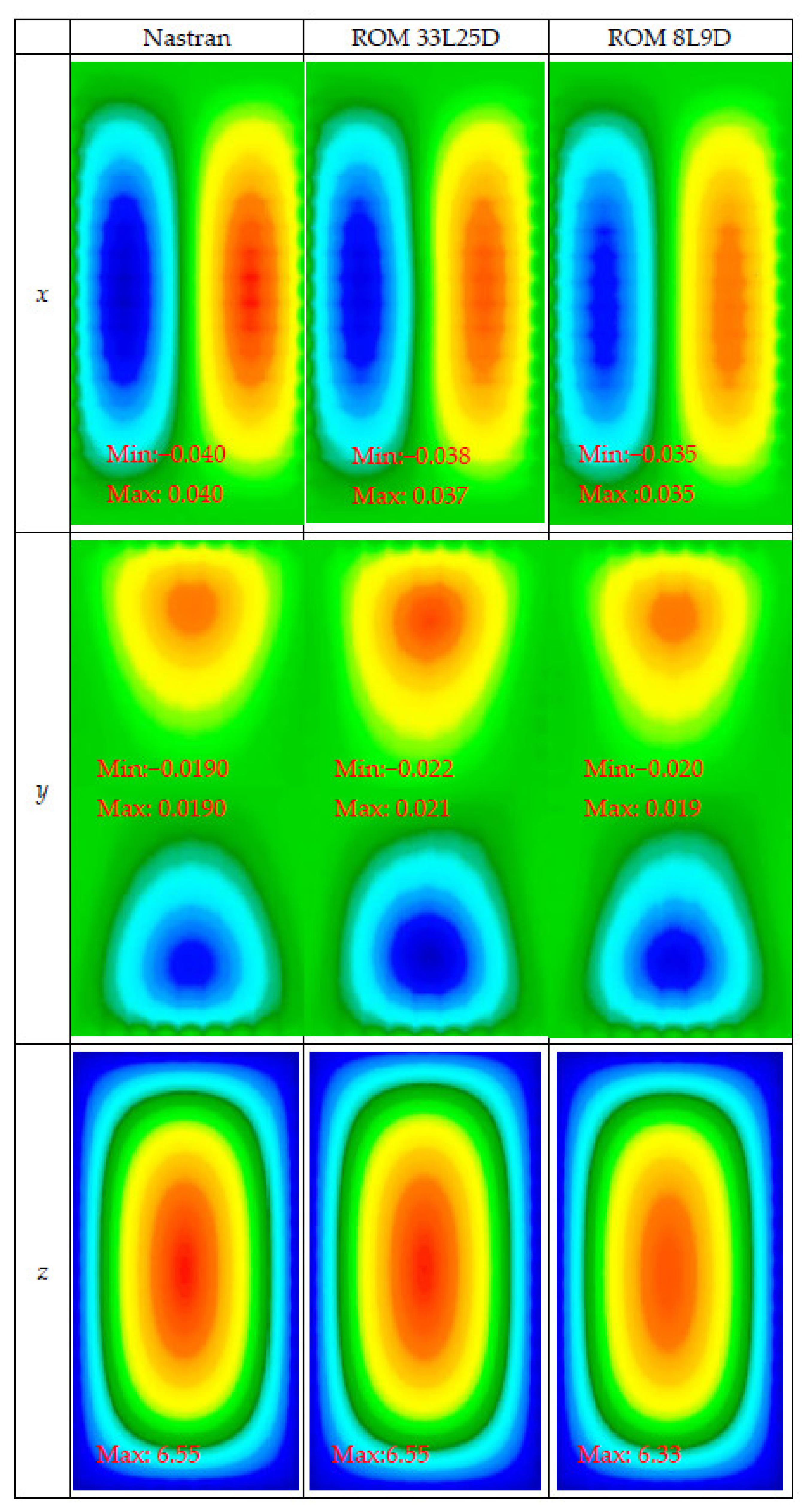
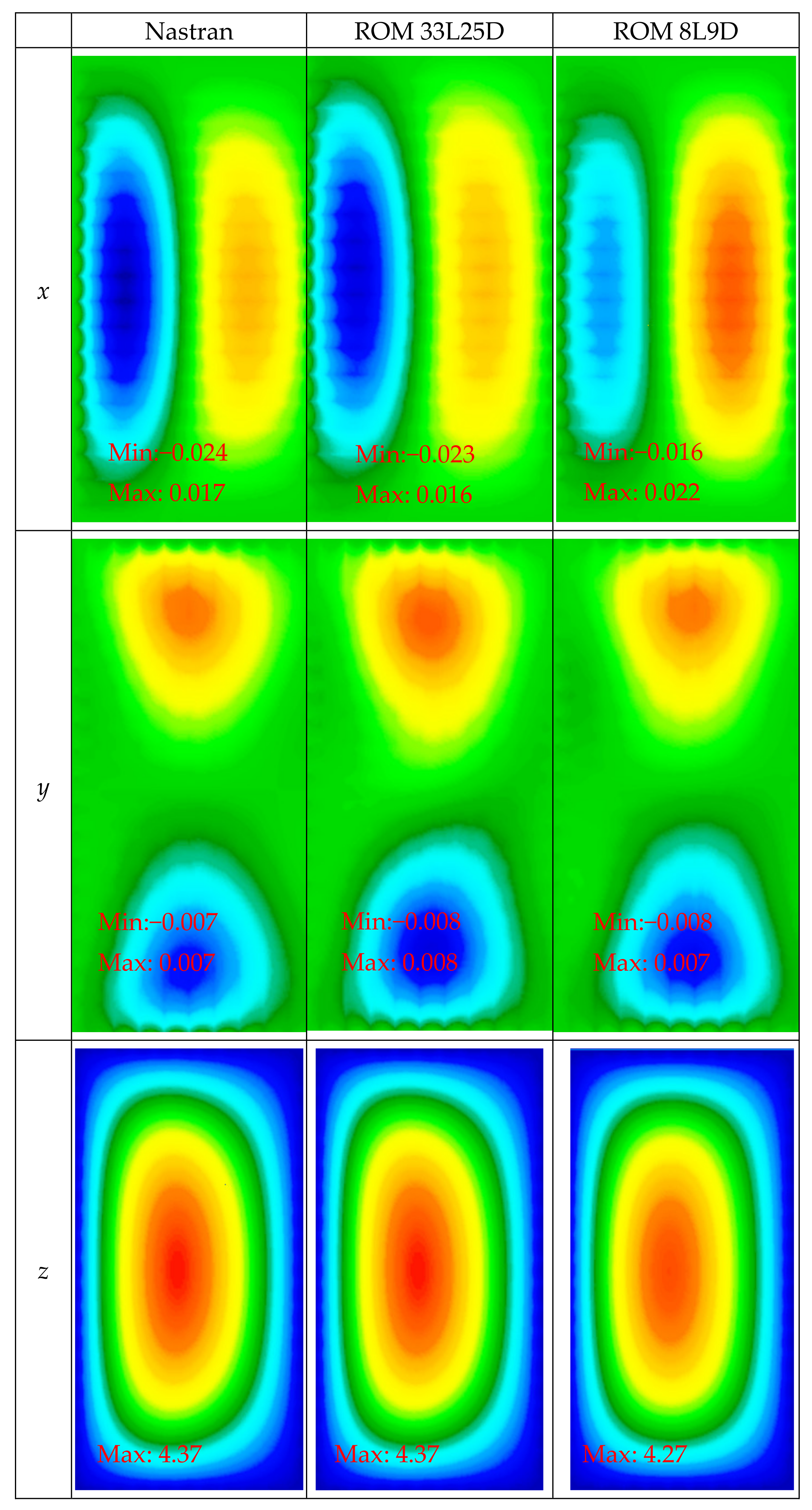
Figure 14 confirms these results by displaying the displacement fields along x, y, and z of the skin at the highest load level of 20 kPa at which the peak transverse displacement is 4.4 thicknesses.
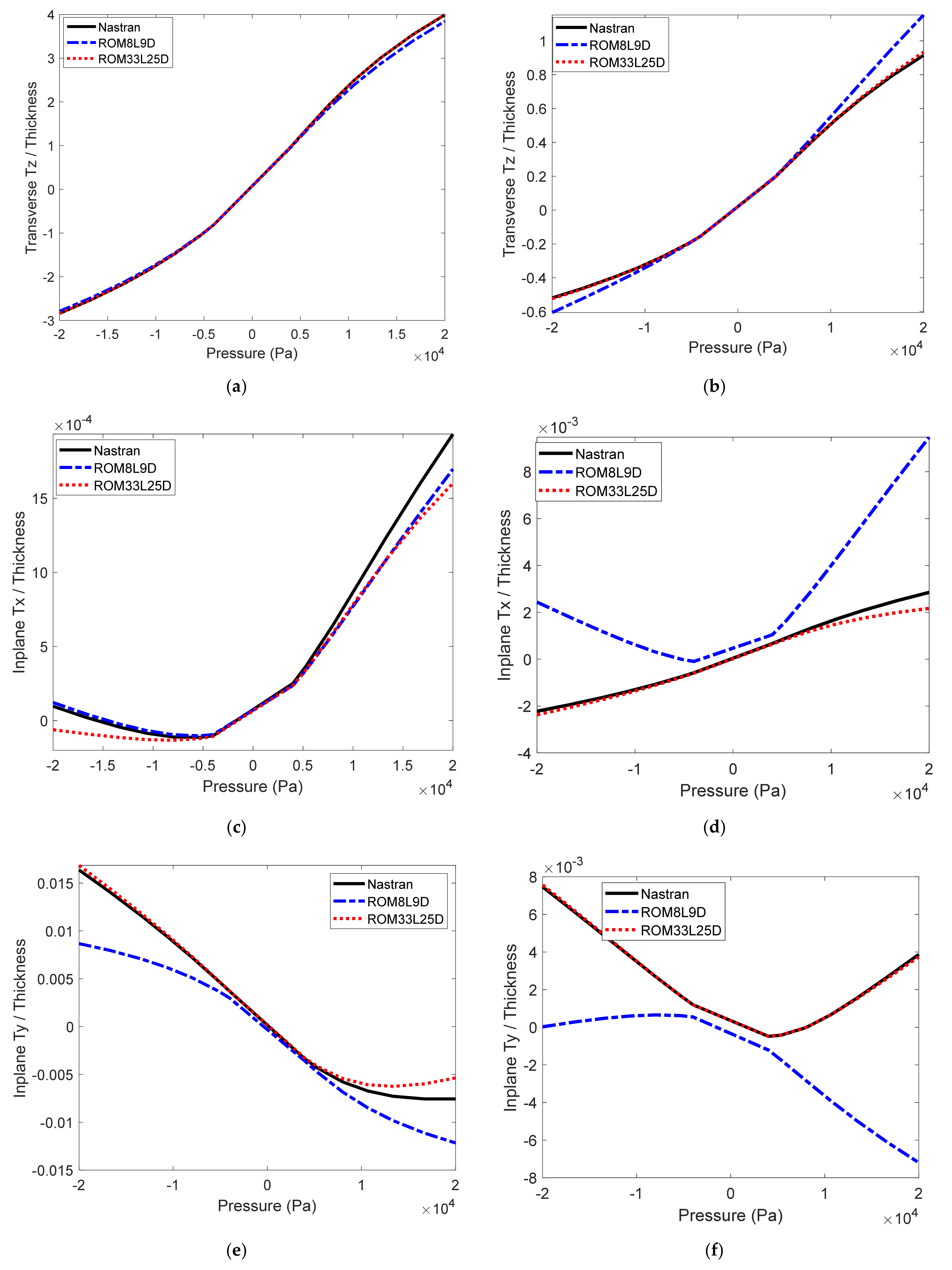
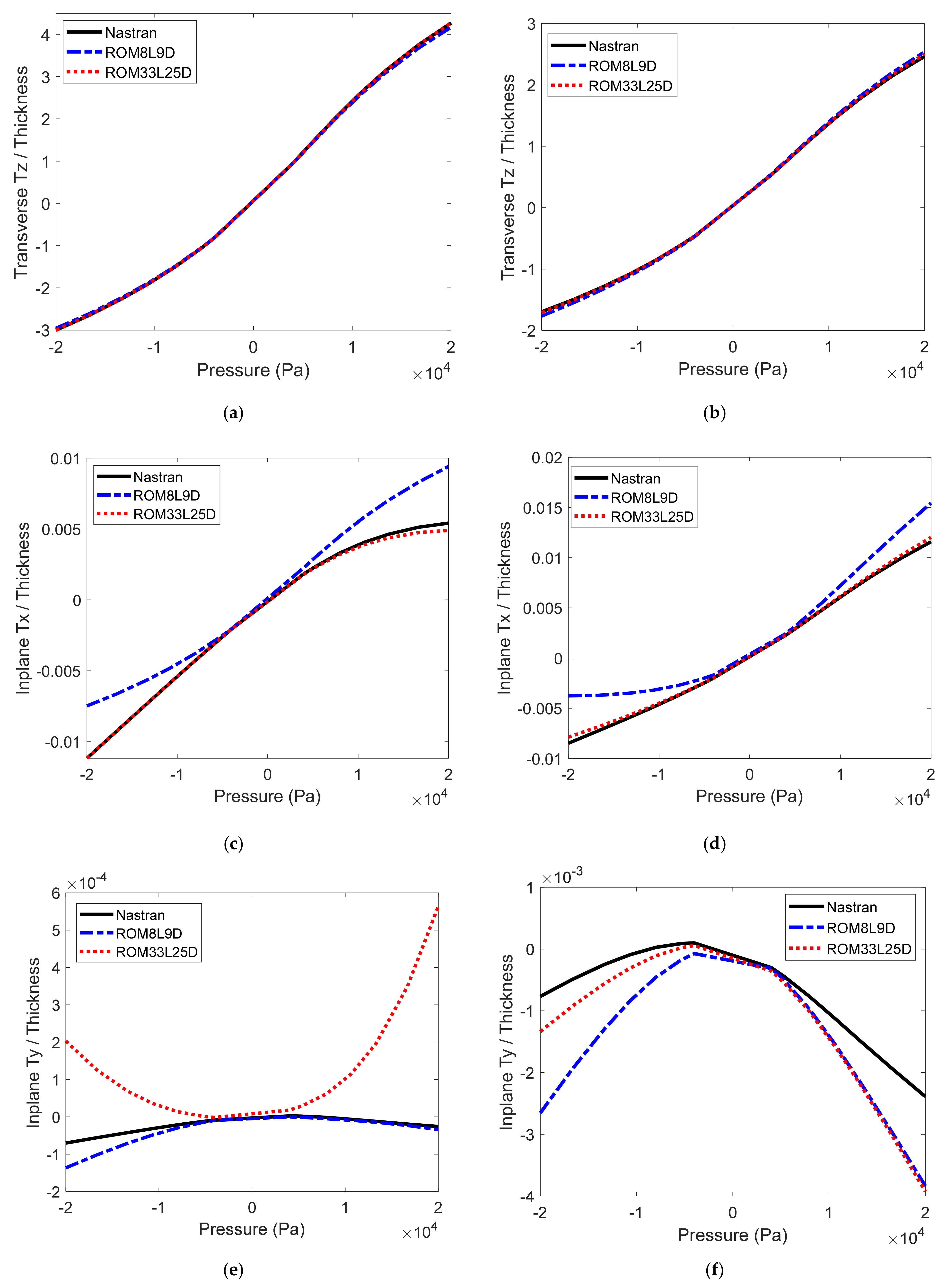
The above validation was repeated for the two asymmetric “split-uniform” pressure distributions of Figure 12, and the corresponding predictions from Nastran and the ROMs are shown in Figure 15, Figure 16, Figure 17 and Figure 18. For these two asymmetric loadings, the 33L25D model still provides excellent predictions of the Nastran responses in all three directions, while the 8L9D model is primarily successful at predicting the transverse displacements with noticeably larger errors on the in-plane displacements.

5. Further Discussions on Basis Construction

5.1. Linear Modes Selection

As discussed in Section 3.1, the selection of the linear modes to be included in nonlinear ROM bases may be more challenging than it is for linear modal analyses, but the static nonlinear responses to the loadings of Equations (3) and (10) or (12)–(13) provide some support in this respect. Indeed, while these loadings are designed to primarily (entirely in the linear case) excite either one or a pair of linear modes, the corresponding responses include a much broader set of them because of the nonlinear static coupling that exists between linear modes. A projection of these responses on a large number of linear modes will thus point to the single or pair of modes excited but also to other modes that are induced by the nonlinear static coupling mechanism. Any large contribution on modes not excited directly would clearly signal modes that will respond because of this coupling. Note that the above discussion and the derivations below are not applicable to the detection of internal resonances that lead to a dynamic, not static, nonlinear coupling between linear modes. Mathematically, the responses w n α n will be approximated by their projections on a set of linear modes, i.e.,
w n α n i = 1 N L η i α n V i
where N L is a “large” number, i.e., much larger than the number of linear modes taken for the linear problem. Since these modes are orthogonal to each other with respect to the mass matrix, the projection coefficients η i α n can be obtained directly by premultiplying Equation (21) by V i T M F E and applying the orthogonality property. This yields
η i α n = V i T M F E   w n α n .
Then, the ratio η i α n / η n α n can be used as a measure of the nonlinear coupling between linear modes n and i when the former is excited at a level α n . Thus, using the data that are already generated to determine the dual modes, one can assess which linear modes i will be excited through the nonlinear coupling with mode n by plotting the values of η i α n / η n α n vs. i. Any large peak of this curve indicates a linear mode that should definitely be considered for inclusion in the basis, even if it is out of band or not excited directly. The static response data generated with loadings of the form of Equations (10) or (13) can be analyzed similarly.
The above analysis permits to explain some observations drawn in earlier investigations, the first one of which relates to the beam of Figure 19 considered in [7]. The beam is made of isotropic elastic material with the following properties: Young’s modulus (E) = 205 MPa, Poisson’s ratio (v) = 0.3, density ( ρ ) = 1966.8 kg/m3. The beam thickness is 7.75 × 10⁻⁴ m, and it is 0.2286 m long and 0.0127 m wide. The springs are identical, with stiffness k = 200 N/m.
It was found in [7] that the nonlinear response of the beam of Figure 19 involved a large contribution of mode 3 even though that in-band mode was almost not directly excited. Moreover, clear contributions of the out of band transverse modes 5–8, 10, and 11 were also observed. To clarify these findings, the data used in [7] to generate the dual modes were analyzed again but, as above, focusing first on mode n = 1, which is the one that is directly excited. The coefficients η i α 1 were then evaluated for the 24 levels α 1 of [7] and for modes i = 1, 2, …, 50, which is much larger than the 4 in-band modes. This plot is shown in Figure 20a and shows clear peaks for the modes 1 (excited), 3, 6, 8, 11 but also mode 34. The coefficients η i α 1 of these modes, normalized by η 1 α 1 , are plotted vs. α 1 on Figure 20b. As expected, at very low excitation levels, the contributions of the non-excited modes are very small. It is also seen that the mode 3 response becomes very significant, which confirms the observations of [7] that this mode is a dominant one.
The plots of Figure 20 justify using linear modes 6, 8, and 11 in the ROM basis but not modes 5, 7, and 10. The absence of these modes is, in fact, due to the symmetry of the system, which leads to transverse modes that are either symmetric or antisymmetric. Modes 1, 3, 6, 8, and 11 are all antisymmetric and do not couple with the symmetric ones, i.e., modes 2, 4, 5, 7, 10. Repeating the above analysis with mode n = 2 leads to the results of Figure 21, which show the coupling with the other key modes, i = 5, 7, and 10.
A similar analysis was also carried out for the hat section panel shown in Figure 22, see [41,42], the material properties of which were selected as: Young’s Modulus of 2 × 10¹¹ Pa, shear modulus of 8 × 10¹⁰ Pa, and density of 7850 kg/m3. Of particular interest here are the modes that are nonlinearly coupled to modes n = 1 and mode n = 6, which are dominant modes in the response. Given the asymmetry of the structure, the loadings of the form of Equation (3) with positive and negative α n , s factors do not lead to opposite projections. Shown in Figure 23 are the normalized projection coefficients for the relevant linear modes, which demonstrate that mode 1 is only very weakly coupled to other linear modes, surprisingly most strongly to the higher frequency mode 18. On the contrary, mode 6 is very strongly coupled to mode 7 but also to mode 10 and, to a notably lower degree, to mode 1. This figure highlights, in particular, the lack of symmetry of the plot for positive and negative loadings when the structure is not symmetric, i.e., the coupling between modes varies with respect to the loading direction. Note finally that the coupling as defined here is not a symmetric property; the projection of the deflections induced by mode i on mode j does not equate to the projection on mode i of the deflections induced on mode j because the load levels α n will be different for these 2 loading scenarios as the level of deflection is controlled, not the force level.

5.2. Selection of the Values α n

Specific directions were given in Section 3.3 to select the load levels α n in Equations (3) and (10). A small updating of these recommendations is provided here based on recent experience. The first change relates to the peak values of α n for different mode numbers n, which were recommended in Section 3.3 to correspond to an identical peak displacement. This rule has led to reliable ROMs but occasionally larger bases than necessary because the deformations induced for higher order, very stiff modes were overly conservative. A more balanced selection focuses not on the peak deflection but rather on the peak stress, i.e., that peak values of α n for different mode numbers n correspond to an identical peak stress dictated by a maximum displacement on the lowest mode of the order of 1-4 thicknesses.
Consistent with this stress perspective, it is suggested here that the parameters α i and α j not be taken equal but rather that α i   ω i 2 = α j   ω j 2 , which leads to approximately equal stresses induced by the two modes i and j.
A second addition to Section 3.3 relates to the signs of α i and α j in Equation (10). Not only should these two parameters admit positive and negative values, as stated in Section 3.3, but these cases should also include equal and opposite signs of α i and α j . This entire dataset corresponding to 2 specific modes is then treated as discussed in Section 2. This selection leads for structures with symmetries to dual that better respect those symmetries than when the signs of α i and α j are always the same.

5.3. Revised Selection of the Number of Eigenvectors as Duals

It was emphasized in Section 3 that the information present in the deflections w n α n must be well captured in constructing the dual modes to obtain a good ROM basis. To this end, the number of POD eigenvectors retained as duals at each step (i.e., for each combination) was dictated by the convergence criterion of either Equations (8) or (9). One aspect that has not been considered to date is that duals that are selected when analyzing later combinations actually improve the representation of the data analyzed for earlier ones, even when the representation error threshold is low. This finding is clearly displayed in Figure 24, which provides the representation error for the duals corresponding to the combinations 1-1, 1-2, 1-3, 1-4, 2-2, and 2-3 for the clamped-clamped beam of Figure 25 and Table 7 at the end of each step, i.e., after taking 2, 3, 2, 1, 2, and 1 duals, respectively, for which convergence was assessed with the criterion of Equation (8) and ε r e p ( t h ) = 0.01.
The implication of the above finding is that the final basis provides a more refined representation of the data that the target of ε r e p ( t h ) = 0.01 and thus may be over conservative, i.e., leading to a ROM basis that may be larger than necessary for that target. Equivalently, this finding suggests that it may not be necessary to take a full set of duals from one combination in order to meet the target of the error threshold strictly, but rather let the duals selected later from other combinations to help reduce the error further.
This perspective leads to a different strategy for the selection of the modes numbers n or i and j considered in Equations (3) and (10). Specifically, rather than taking a limited number of combinations following the informed arguments of Section 3.2, the displacements of which are analyzed until strict convergence, one could consider a much broader, more straightforward set of combinations and tentatively take only a limited number (say 1 or 2) of POD eigenvectors (with largest energy measure) as duals. However, to ensure that all the information present in the deflections w n α n has been well captured at the end, a revisit at that time of the entire set of data (i.e., for all combinations) should be carried out and additional POD steps should be reformulated for combinations not meeting the target threshold ε r e p ( t h ) .
In summary, this new strategy proceeds as follows:
(i)
select a broad set of combinations of 1 and 2 modes
(ii)
for each combination, analyze the data using Equations (4)–(7) and take the 1 or 2 POD eigenvectors with largest strain measure or largest drop in representation error as dual.
(iii)
when all combinations have been treated, recompute the representation error of the data for each combination with the obtained basis.
(iv)
for any combination with representation error in (iii) larger than the threshold of ε r e p ( t h ) , determine the residuals U n , s or U i , j , s of the corresponding data with the final basis and proceed with a POD to decrease the representation error to below ε r e p ( t h ) .
The process (i)–(iv) will lead to a basis that achieves the target threshold of ε r e p ( t h ) on all combinations and is expected to have a smaller number of duals than using previous approaches of Section 3 and Section 3.2. Moreover, it will cover a broader set of combinations requiring less informed decision as before and thus leads to a more automatic construction of the dual modes.
Before demonstrating this new process in the following section, it should be noted that a single POD of the entire data of all combinations taken together could be carried out. This effort has been compared to the process (i)–(iv) and does not appear to lead to a smaller basis. Yet, the analysis of each combination alone is advantageous because it is fully expected that some combinations are more likely than others to be important, e.g., combinations involving lower order modes vs. those of higher order. This information is rather intuitive and is more challenging to introduce mathematically (through a weighting matrix) in a single POD framework.

5.4. Beam with Narrowly Distributed Loading

Most mechanical loading conditions (i.e., excluding heating) considered in previous investigations have been either distributed over the entire structure and generally uniformly or concentrated forces. To enrich this set of validations, the beam of Figure 25 is considered here with a uniform loading only over the left 1/4 of its length, which is either static or dynamic. It is desired to construct a ROM appropriate for an excitation band of [0, 1000] Hz, which includes the first 5 linear modes of frequencies 79.63, 219.49, 430.23, 711.09, 845.13 Hz. For the static loading, the consideration of these 5 linear modes also appears appropriate based on a linear analysis.
Following the discussion of Section 5.3, the dual modes were selected from the full set of combinations of modes 1-4, i.e., 1-1, 1-2, 1-3, 2-2, 1-4, 2-3, 2-4, 3-3, 3-4, 4-4 in this order, which reflects the relative magnitudes of the modes in the linear case. Mode 5 was only present minimally in the linear response and thus was not included in the dual selection. The displacement data used was in the range of 0.01 to 1.5–2.0 thicknesses with the load factors α i and α j spanning both positive and negative values and with both equal and opposite signs, see Section 5.2. For each combination, the POD eigenvector with the largest contribution to the total potential energy of the displacement data was selected as the dual leading to a 5L10D ROM. Figure 26 shows the evolution of the representation errors for the first 6 combinations as a function of the number of duals selected. It is clearly seen, as in Figure 24, that taking duals for later combinations does also reduce the error for earlier ones.
As discussed in Section 5.3, the next step is to check the representation errors of the 10 combinations and their maximum values are show on Table 8. It is clearly seen that these errors are not below the threshold of 1% for some of the combinations and for both transverse and in-plane directions. This situation will be remedied by reconsidering successively the data of the combinations with a representation error above the threshold and selecting as many duals as necessary to lower this error to below the 1% threshold. The representation errors of the 10 combinations will then be recomputed and any combination with a representation error larger than 1% will again be used to obtain new duals. This process was carried out first with the combination 1-4, which does not have the largest representation error but involves a key low frequency mode. A single POD eigenvector was selected and the representation errors with this 5L11D model were recomputed. At this point, the combination 4-4 remained the only one with a representation error above 1%, 1.44% specifically, and a POD of its residuals after projection on the 5L11D basis was carried out. The selection of the eigenvector with the largest strain measure as 12th dual led to a drop of the error below 1% for that combination as well, ending the selection of dual modes.
The reduction in the representation errors in the transverse direction was achieved by adding the linear modes most effective in reducing the representation error, which were determined by checking the curves of transverse representation error versus the number of linear modes for all the 10 combinations. In this process, the linear modes 6, 8, 10, 11, 13, 16, 18, and 20 were added for a final ROM with 12 linear modes and 12 duals.
Both the 5L10D and 12L12D ROMs were identified using the tangent stiffness approach of [4] and an assessment of the accuracy of their predictions was performed on the quarter beam loading of Figure 25 both in static and dynamic conditions. For the former, 3 loading levels were considered that lead to peak transverse displacements of 0.1, 0.75, and 2.5 thicknesses, i.e., low, medium, and high levels of nonlinearity. The corresponding values of the pressure were 4, 50, and 500 N/m, which is indeed seen to increase significantly faster than the peak transverse displacement level. Similarly, the peak in-plane displacements of 3 × 10⁻⁵, 3 × 10⁻³, and 0.04 thickness increase much faster than the peak transverse ones, approximately quadratically.
The comparison of the static deformed shapes, in the transverse and in-plane directions, is shown in Figure 27, and it is seen that the agreement is excellent for all levels with the 5L10D ROM. The corresponding results obtained with the 12L12D ROM are essentially identical to the finite element ones.
For the dynamic validation, the time dependence of the loading was modeled as a bandlimited white noise in the frequency band [0, 1000] Hz and its magnitude was selected to yield a standard deviation of the peak transverse displacement of 0.72 thickness. Moreover, the coefficients of the Rayleigh damping were selected as α = 12.838/s and β = 2.061 × 10⁻⁶ s which led to damping ratios of 1.4%, 0.6%, 0.5%, 0.5%, and 0.6% on the first 5 linear modes. Then, shown in Figure 28 is a comparison of the power spectra at the middle and quarter points in both transverse and in-plane directions between the finite element predictions and those corresponding to the 5L10D and 12L12D ROMs. It is seen that the 5L10D model provides an excellent prediction over the excitation band, up to 1500 Hz and a good one, especially for the in-plane displacements, from 1500 Hz to 3000 Hz, which is significantly above the excitation band. Also shown on these figures are the predictions obtained from the 12L12D and they match the finite element ones very closely up to 3000 Hz. The inclusion of the extra, out of band, linear modes and duals has thus led to the capture of the response not only in the excitation band but well above it. This richer model thus permits to also capture accurately the out of band transfer of energy that takes place. The excellent accuracy of the 5L10D model results from the low representation errors of the dual data, see Table 8, over a broad ensemble of combinations that include the 4 most significant modes.
In the POD strategy of Section 5.3, a dual derived from any loading combination provides, in general, a reduction in the representation error for other loading conditions. Thus, increasing the number of combinations to consider does not necessarily lead to a similar increase in the number of duals. For example, considering the 15 combinations that involve all 5 modes in band, i.e., 1-1, 1-2, 1-3, 2-2, 1-4, 2-3, 2-4, 3-3, 3-4, 4-4, 1-5, 2-5, 3-5, 4-5, and 5-5 leads after selecting 1 eigenvector as dual for each combination to representation errors on all 15 combinations that are below 1%. So, the consideration of 5 extra combinations has led to only adding 3 more duals. The corresponding 12L15D was also identified and its predictions of the static and dynamic loading conditions of Figure 27 and Figure 28 are very close to those of the 12L12D.

6. Summary

The focus of this investigation has been on complementing the existing work on reduced order modeling for the nonlinear geometric response of structures by, first, providing clarifications and recommendations for the determination of the basis and, second, by demonstrating the validity and accuracy of this approach to four novel, atypical structures. The basis used here is composed of a series of linear modes of the structures enriched by dual modes that represent the membrane stretching induced by the large displacements. Existing aspects of the construction of the dual modes are first reviewed in detail, but newer aspects are also presented, the most important of which is how the POD process involved in this construction is performed. This new process considers a broad set of loading combinations and takes a limited, e.g., one, eigenvector from each as a dual mode to form a first set of them. Once a first pass through this data has been completed, a revisit of the representation errors is carried out and additional POD steps are performed as needed to ensure that the representation error for all the combinations is lower than the desired threshold. This new strategy is expected to provide a more compact basis given a set of loading conditions or permits to model a broader set of those with the same basis size.
It is shown next that a by-product of the construction of the duals is data that permit to estimate the nonlinear coupling that exists between linear modes. This information is particularly useful in selecting which linear modes, especially out of band ones, must be included in the basis.
The above existing and novel basis construction strategies are applied to four novel structural problems that have atypical geometry, boundary conditions, or loading. These include a freely expanding plate, an orthogrid panel of complex geometry, and a beam loaded only on one quarter of its length. For each case, the construction of the basis is detailed, and comparisons of the static and/or dynamic response predictions from both the ROMs and the underlying finite element model are carried out for strongly nonlinear responses. The excellent match between the finite element and ROM predictions in all cases demonstrates the high accuracy that can be achieved with the proposed ROMs.

Author Contributions

Metholodogy: X.W. and M.P.M.; Validation, X.W., R.A.P., B.W. and Y.W. All authors have read and agreed to the published version of the manuscript.

Funding

This research was partially funded by the Air Force Office of Scientific Research (grant FA9550-07-1-0031 with V. Giurgiutiu as grant monitor), the AFRL-University Collaborative Center in Structural Sciences (Cooperative Agreement FA8650-13-2347 with B. Smarslok as Program Manager), and the Boeing Company.

Data Availability Statement

The data and the ASU developed models are freely available from the corresponding author. The codes are intellectual property of the Arizona Board of Regents and require intellectual property transfer approval.

Acknowledgments

The authors sincerely thank A. Gogulapati and J.J. MacNamara for the use of the orthogrid finite element model.

Conflicts of Interest

The authors declare no conflict of interest.

References

  1. Mignolet, M.P.; Przekop, A.; Rizzi, S.A.; Spottswood, S.M. A Review of Indirect/Non-Intrusive Reduced Order Modeling of Nonlinear Geometric Structures. J. Sound Vib. 2013, 332, 2437–2460. [Google Scholar] [CrossRef]
  2. Hollkamp, J.J.; Gordon, R.W.; Spottswood, S.M. Nonlinear Modal Models for Sonic Fatigue Response Prediction: A Comparison of Methods. J. Sound Vib. 2005, 284, 1145–1163. [Google Scholar] [CrossRef]
  3. Kim, K.; Radu, A.; Wang, X.Q.; Mignolet, M.P. Nonlinear Reduced Order Modeling of Isotropic and Functionally Graded Plates. Int. J. Non-Linear Mech. 2013, 49, 100–110. [Google Scholar] [CrossRef]
  4. Perez, R.A.; Wang, X.Q.; Mignolet, M.P. Non-Intrusive Structural Dynamic Reduced Order Modeling for Large Deformations: Enhancements for Complex Structures. J. Comput. Nonlinear Dyn. 2014, 9, 031008. [Google Scholar] [CrossRef]
  5. Spottswood, S.M.; Hollkamp, J.J.; Eason, T.G. Reduced-Order Models for a Shallow Curved Beam Under Combined Loading. AIAA J. 2010, 48, 47–55. [Google Scholar] [CrossRef]
  6. Przekop, A.; Guo, X.; Rizzi, S.A. Alternative modal basis selection procedures for reduced-order nonlinear random response simulation. J. Sound Vib. 2012, 331, 4005–4024. [Google Scholar] [CrossRef]
  7. Wang, Y.; Wang, X.Q.; Mignolet, M.P. Component-Centric Reduced Order Modeling for the Prediction of the Nonlinear Geometric Response of a Part of a Stiffened Structure. J. Comput. Nonlinear Dyn. 2018, 13, 121006. [Google Scholar] [CrossRef]
  8. Perez, R.A.; Wang, X.Q.; Mignolet, M.P. Prediction of Displacement and Stress Fields of a Notched Panel with Geometric Nonlinearity by Reduced Order Modeling. J. Sound Vib. 2014, 333, 6572–6589. [Google Scholar] [CrossRef] [Green Version]
  9. Wang, X.Q.; Phlipot, G.P.; Perez, R.A.; Mignolet, M.P. Locally Enhanced Reduced Order Modeling for the Nonlinear Geometric Response of Structures with Defects. Int. J. Non-Linear Mech. 2018, 101, 1–7. [Google Scholar] [CrossRef]
  10. O’Hara, P.J.; Hollkamp, J.J. Modeling Vibratory Damage with Reduced-Order Models and the Generalized Finite Element Method. J. Sound Vib. 2014, 333, 6637–6650. [Google Scholar] [CrossRef]
  11. Wang, X.Q.; O’Hara, P.J.; Mignolet, M.P.; Hollkamp, J.J. Reduced Order Modeling with Local Enrichment for the Nonlinear Geometric Response of a Cracked Panel. AIAA J. 2019, 57, 421–436. [Google Scholar] [CrossRef]
  12. Kuether, R.J.; Allen, M.S.; Hollkamp, J.J. Modal Substructuring of Geometrically Nonlinear Finite-Element Models. AIAA J. 2016, 54, 691–702. [Google Scholar] [CrossRef] [Green Version]
  13. Kuether, R.J.; Allen, M.S.; Hollkamp, J.J. Modal Substructuring of Geometrically Nonlinear Finite Element Models with Interface Reduction. AIAA J. 2017, 55, 1695–1706. [Google Scholar] [CrossRef]
  14. Mahdiabadi, M.K.; Bartl, A.; Xu, D.; Tiso, P.; Rixen, D.J. An Augmented Free-Interface-Based Modal Substructuring for Nonlinear Structural Dynamics Including Interface Reduction. J. Sound Vib. 2019, 462, 114915. [Google Scholar] [CrossRef]
  15. Kuether, R.J.; Deaner, B.J.; Hollkamp, J.J.; Allen, M.S. Evaluation of Geometrically Nonlinear Reduced-Order Models with Nonlinear Normal Modes. AIAA J. 2015, 53, 3273–3285. [Google Scholar] [CrossRef]
  16. Gordon, R.W.; Hollkamp, J.J. Reduced-Order Models for Acoustic Response Prediction of a Curved Panel. In Proceedings of the 52nd AIAA/ASME/ASCE/AHS/ASC Structures, Structural Dynamics and Materials Conference, Denver, CO, USA, 4–7 April 2011. [Google Scholar] [CrossRef]
  17. Hollkamp, J.J.; Perez, R.A.; Spottswood, S.M. Design Sensitivities of Components Using Nonlinear Reduced-Order Models and Complex Variables. In Proceedings of the International Modal Analysis Conference (IMAC XXXV), Garden Grove, CA, USA, 30 January–2 February 2017. [Google Scholar] [CrossRef]
  18. Perez, R.; Bartram, G.; Beberniss, T.; Wiebe, R.; Spottswood, S.M. Calibration of Aero-Structural Reduced Order Models using Full-Field Experimental Measurements. Mech. Syst. Signal Processing 2017, 86, 49–65. [Google Scholar] [CrossRef]
  19. Wiebe, R.; Perez, R.A.; Spottswood, S.M. Robust Simulation of Buckled Structures using Reduced Order Modeling. J. Phys. Conf. Ser. 2016, 744, 012118. [Google Scholar] [CrossRef] [Green Version]
  20. Givois, A.; Grolet, A.; Thomas, O.; Deü, J.-F. On the Frequency Response Computation of Geometrically Nonlinear Flat Structures using Reduced-Order Finite Element Models. Nonlinear Dyn. 2019, 97, 1747–1781. [Google Scholar] [CrossRef] [Green Version]
  21. Wang, X.Q.; Khanna, V.; Kim, K.; Mignolet, M.P. Nonlinear Reduced Order Modeling of Flat Cantilevered Structures: Challenges and Remedies. ASCE J. Aerosp. Eng. 2021, 34, 04021085. [Google Scholar] [CrossRef]
  22. Wang, X.Q.; Song, P.; Mignolet, M.P.; Chen, P.C. Reduced Order Nonlinear Damping Model: Formulation and Application to Post-Flutter Aeroelastic Behavior. AIAA J. 2021, 59, 4144–4154. [Google Scholar] [CrossRef]
  23. Mahdiabadi, M.K.; Tiso, P.; Brandt, A.; Rixen, D.J. A Non-Intrusive Model-Order Reduction of Geometrically Nonlinear Structural Dynamics Using Modal Derivatives. Mech. Syst. Signal Processing 2021, 147, 107126. [Google Scholar] [CrossRef]
  24. Wang, X.Q.; Mignolet, M.P. Discussion on ‘A Non-Intrusive Model-Order Reduction of Geometrically Nonlinear Structural Dynamics Using Modal Derivatives’. Mech. Syst. Signal Processing 2021, 159, 107638. [Google Scholar] [CrossRef]
  25. Wang, X.Q.; Mignolet, M.P. Toward a Systematic Construction of the Basis for Nonlinear Geometric Reduced Order Models. In Proceedings of the 11th International Conference on Structural Dynamics (EURODYN 2020), Athens, Greece, 23–25 November 2020; Available online: https://eurodyn2020.org/proceedings/ (accessed on 19 August 2021).
  26. Vizzaccaro, A.; Givois, A.; Longobardi, P.; Shen, Y.; Deü, J.-F.; Salles, L.; Touzé, C.; Thomas, O. Non-Intrusive Reduced Order Modelling for the Dynamics of Geometrically Nonlinear Flat Structures using Three-Dimensional Finite Elements. Comput. Mech. 2020, 66, 1293–1319. [Google Scholar] [CrossRef]
  27. Shen, Y.; Vizzaccaro, A.; Kesmia, N.; Yu, T.; Salles, L.; Thomas, O.; Touzé, C. Comparison of Reduction Methods for Finite Element Geometrically Nonlinear Beam Structures. Vibration 2021, 4, 175–204. [Google Scholar] [CrossRef]
  28. Givois, A.; Deü, J.-F.J.; Thomas, O. Dynamics of Piezoelectric Structures with Geometric Nonlinearities: A Non-Intrusive Reduced Order Modelling Strategy. Comput. Struct. 2021, 253, 106575. [Google Scholar] [CrossRef]
  29. Marconi, J.; Tiso, P.; Braghin, F. A Nonlinear Reduced Order Model with Parametrized Shape Defects. Comput. Methods Appl. Mech. Eng. 2020, 360, 112785. [Google Scholar] [CrossRef]
  30. Van Damme, C.I.; Allen, M.S.; Hollkamp, J.J. Updating Geometrically Nonlinear Reduced-Order Models Using Nonlinear Modes and Harmonic Balance. AIAA J. 2020, 58, 3553–3568. [Google Scholar] [CrossRef]
  31. Van Damme, C.I.; Allen, M.S.; Hollkamp, J.J. Evaluating Reduced Order Models of Curved Beams for Random Response Prediction Using Static Equilibrium Paths. J. Sound Vib. 2020, 468, 115018. [Google Scholar] [CrossRef]
  32. Shen, Y.; Béreux, N.; Frangi, A.; Touzé, C. Reduced Order Models for Geometrically Nonlinear Structures: Assessment of Implicit Condensation in Comparison with Invariant Manifold Approach. Eur. J. Mech. A/Solids 2021, 86, 104165. [Google Scholar] [CrossRef]
  33. Phlipot, G.; Wang, X.Q.; Mignolet, M.P.; Demasi, L.; Cavallaro, R. Nonintrusive Reduced Order Modeling for the Nonlinear Geometric Response of Some Joined Wings. In Proceedings of the AIAA Science and Technology Forum and Exposition (SciTech2014), National Harbor, MD, USA, 13–17 January 2014. [Google Scholar] [CrossRef]
  34. Kim, E.; Cho, M. Equivalent Model Construction for a Non-Linear Dynamic System Based on an Element-Wise Stiffness Evaluation Procedure and Reduced Analysis of the Equivalent System. Comput. Mech. 2017, 60, 709–724. [Google Scholar] [CrossRef]
  35. Lulf, F.; Tran, D.M.; Matthies, H.G.; Ohayon, R. An Integrated Method for the Transient Solution of Reduced Order Models of Geometrically Nonlinear Structures. Comput. Mech. 2015, 55, 327–344. [Google Scholar] [CrossRef]
  36. Mignolet, M.P.; Soize, C. Stochastic Reduced Order Models for Uncertain Geometrically Nonlinear Dynamical Systems. Comput. Methods Appl. Mech. Eng. 2008, 197, 3951–3963. [Google Scholar] [CrossRef] [Green Version]
  37. Matney, A.; Spottswood, S.M.; Mignolet, M.P. Nonlinear Structural Reduced Order Modeling Methods for Hypersonic Structures. In Proceedings of the 53rd Structures, Structural Dynamics and Materials Conference, Honolulu, HI, USA, 23–26 April 2012. [Google Scholar] [CrossRef]
  38. Murthy, R.; Wang, X.Q.; Perez, R.; Mignolet, M.P.; Richter, L.A. Uncertainty-Based Experimental Validation of Nonlinear Reduced Order Models. J. Sound Vib. 2012, 331, 1097–1114. [Google Scholar] [CrossRef]
  39. Muravyov, A.A.; Rizzi, S.A. Determination of Nonlinear Stiffness with Application to Random Vibration of Geometrically Nonlinear Structures. Comput. Struct. 2003, 81, 1513–1523. [Google Scholar] [CrossRef]
  40. Kerschen, G.; Golinval, J.-C.; Vakakis, A.F.; Bergman, L.A. The Method of Proper Orthogonal Decomposition for Dynamical Characterization and Order Reduction of Mechanical Systems: An Overview. Nonlinear Dyn. 2005, 41, 147–169. [Google Scholar] [CrossRef]
  41. Wainwright, B.A.; Wang, X.Q.; Mignolet, M.P. Investigation of Out-of-Band Response in Reduced Order Models of Nonlinear Geometric Response. In Proceedings of the International Modal Analysis Conference (IMAC XXXVIII), Houston, TX, USA, 10–13 February 2020. [Google Scholar]
  42. Wainwright, B.A.; Wang, X.Q.; Mignolet, M.P. Nonlinear Reduced Order Modeling for the Dynamic Response of a Built-up Structure with Strong Asymmetry through Thickness. In Proceedings of the International Modal Analysis Conference (IMAC XXXVII), Orlando, FL, USA, 28–31 January 2019. [Google Scholar]
  43. Spottswood, S.M.; Eason, T.G.; Wang, X.Q.; Mignolet, M.P. Nonlinear Reduced Order Modeling of Curved Beams: A Comparison of Methods. In Proceedings of the 50th Structures, Structural Dynamics, and Materials Conference, Palm Springs, CA, USA, 4–7 May 2009. [Google Scholar] [CrossRef]
  44. Lin, J.; Wang, X.Q.; Mignolet, M.P. On the Detection and Capturing of Strongly Nonlinear Geometric Events with Reduced Order Models. In Proceedings of the International Modal Analysis Conference (IMAC XXXVIII), Houston, TX, USA, 10–13 February 2020. [Google Scholar]
  45. Lin, J.; Wang, X.Q.; Mignolet, M.P. Nonlinear Reduced Order Modeling of a Cylindrical Shell Exhibiting Mode Veering and Symmetry Breaking. In Proceedings of the International Modal Analysis Conference (IMAC XXXVII), Orlando, FL, USA, 28–31 January 2019. [Google Scholar]
  46. Quiroz, R.; Embler, J.; Jacobs, R.; Tzong, G.; Liguore, S. Predictive Capability for Hypersonic Structural Response and Life Prediction, Phase II Detailed Design of Hypersonic Cruise Vehicle Hot-Structure. Air Force Technical Report AFRL-RQ-WP-TR-2012-0265. 2012. Available online: https://apps.dtic.mil/sti/citations/ADA564197 (accessed on 19 August 2021).
  47. Gogulapati, A.; Brouwer, K.; Wang, X.Q.; Murthy, R.; McNamara, J.J.; Mignolet, M.P. Full and Reduced Order Aerothermoelastic Modeling of Built-Up Aerospace Panels in High-Speed Flows. In Proceedings of the AIAA Science and Technology Forum and Exposition (SciTech2017), Dallas, TA, USA, 9–13 January 2017. [Google Scholar] [CrossRef]
  48. Soize, C. Uncertainty Quantification: An Accelerated Course in Advanced Applications in Computational Engineering; Springer: Berlin/Heidelberg, Germany, 2017. [Google Scholar]
  49. Soize, C. A Nonparametric Model of Random Uncertainties for Reduced Matrix Models in Structural Dynamics. Probabilistic Eng. Mech. 2000, 15, 277–294. [Google Scholar] [CrossRef] [Green Version]
Figure 1. Cantilevered curved beam geometry.
Vibration 05 00002 g001
Figure 2. Deflections of the tip of the cantilevered curved beam as a function of the magnitude of a uniformly distributed static load (positive down). Nastran and ROM predictions. (a) Transverse, (b) in-plane.
Vibration 05 00002 g002
Figure 3. Power spectral densities of the deflections of the tip of the cantilevered curved beam Nastran and ROM predictions for uniformly distributed pressure bandlimited in [0, 100] Hz and with magnitudes of 80 and 90dB. (a) Transverse, (b) in-plane.
Vibration 05 00002 g003
Figure 4. Boundary conditions of freely expanding plate.
Vibration 05 00002 g004
Figure 5. Finite element mesh representation of freely expanding plate. The black dots are the nodes at which the in-plane boundary conditions are imposed.
Vibration 05 00002 g005
Figure 6. Power spectral densities of the responses predicted by Nastran and the ROM. Freely expanding plate under an excitation of OASPL = 147 dB. (a,b) In-plane x and y displacements of the bottom left corner, (c) transverse displacement of panel center.
Vibration 05 00002 g006
Figure 7. Displacements predicted by Nastran and the ROM 6L7D. Freely expanding plate, uniform pressures of 6000 and 12,000 Pa. Displacements of the nodes along the (a,b) middle y = 0 line in the (a) x (in-plane) and (b) z (transverse) directions, (c,d) middle x = 0 line in the (c) y (in-plane) and (d) z (transverse) directions.
Vibration 05 00002 g007
Figure 8. Power spectral densities of the transverse responses of the panel center predicted by Nastran for the freely expanding plate and its fully clamped counterpart under an excitation of OASPL = 147 dB.
Vibration 05 00002 g008
Figure 9. Orthogrid panel (a) perspective view of the underside, (b) zoom of (a) near corner, and (c) cross-section showing the skin (in blue) and a tapered stiffener (in white).
Vibration 05 00002 g009
Figure 10. Structure of the random H K matrices with n = 8, i = 2, and μ = 4.5 and 13.5.
Vibration 05 00002 g010
Figure 11. Uncertainty band (in yellow) of linear frequency responses of the random linear ROM samples to uniform pressure load. (a) Three locations on the panel where the uncertainty band results are shown; (b) center point, (c) quarter point, and (d) edge point. The red lines indicate the natural frequencies of the deterministic orthogrid.
Vibration 05 00002 g011
Figure 12. Asymmetric pressure distributions on the orthogrid panel.
Vibration 05 00002 g012
Figure 13. Static displacements induced by a uniform pressure on the orthogrid panel. Predictions from Nastran and the 8L9D and 33L25D ROMs. (a,c,e) center point, (b,d,f) quarter point, displacements along (a,b) transverse z, (c,d) in-plane x, (e,f) in-plane y.
Vibration 05 00002 g013
Figure 14. Displacement fields along x, y, and z of the skin predicted by Nastran and by the 33L25D and 8L9D ROMs in units of thickness. Uniform pressure of magnitude +20 kPa.
Vibration 05 00002 g014
Figure 15. Static displacements induced by a fore-aft asymmetric pressure on the orthogrid panel. Predictions from Nastran and the 8L9D and 33L25D ROMs. (a,c,e) center point, (b,d,f) quarter point, displacements along (a,b) transverse z, (c,d) in-plane x, (e,f) in-plane y.
Vibration 05 00002 g015
Figure 16. Displacement fields along x, y, and z of the skin predicted by Nastran and the 33L25D and 8L9D ROMs in units of thickness. Fore-aft asymmetric pressure of magnitude +20 kPa.
Vibration 05 00002 g016
Figure 17. Static displacements induced by a left-right asymmetric pressure on the orthogrid panel. Predictions from Nastran, the 8L9D and 33L25D ROMs. (a,c,e) center point, (b,d,f) quarter point, displacements along (a,b) transverse z, (c,d) in-plane x, (e,f) in-plane y.
Vibration 05 00002 g017
Figure 18. Displacement fields along x, y, z of the skin predicted by Nastran and by the 33L25D and 8L9D ROMs in units of thickness. Left-right asymmetric pressure of magnitude +20 kPa.
Vibration 05 00002 g018
Figure 19. The clamped-clamped beam model supported by linear springs of [7].
Vibration 05 00002 g019
Figure 20. Projection coefficients η i α 1 of the static responses w 1 α 1 . Beam on spring supports from Figure 19. (a) η i α 1 vs. linear mode i for all load levels α 1 , s . (b) Normalized coefficients η i α 1 / η 1 α 1 vs. load level α 1 , s for selected modes i = 3, 6, 8, 11, and 34.
Vibration 05 00002 g020
Figure 21. Projection coefficients η i α 2 of the static responses w 2 α 2 . Beam on spring supports from Figure 19. (a) η i α 2 vs. linear mode i for all load levels α 2 , s . (b) Normalized coefficients η i α 2 / η 2 α 2 vs. load level α 2 , s for selected modes i = 4, 5, 7, and 10.
Vibration 05 00002 g021
Figure 22. Hat stiffened panel geometry, boundary conditions, and finite element model.
Vibration 05 00002 g022
Figure 23. Normalized projection coefficients η i α n / η n α n of the static responses w n α n vs. load level α n , s for selected linear modes i, hat section of Figure 22. Mode (a) n = 1, (b) n = 6.
Vibration 05 00002 g023
Figure 24. Representation errors of the combinations 1-1, 1-2, 1-3, 1-4, 2-2, and 2-3 at the end of the POD analysis for each of these combinations taking 2, 3, 2, 1, 2, and 1 duals.
Vibration 05 00002 g024
Figure 25. Clamped-clamped straight beam and loading.
Vibration 05 00002 g025
Figure 26. Representation errors of the combinations 1-1, 1-2, 1-3, 1-4, 2-2, and 2-3 as a function of the number of duals taken—1 dual per combination.
Vibration 05 00002 g026
Figure 27. Static deformed shapes, clamped straight beam loaded on left quarter. Nastran and ROM predictions for different load levels. (a,c,e) Transverse displacements, (b,d,f) in-plane displacements.
Vibration 05 00002 g027
Figure 28. Power spectral densities of the responses predicted by Nastran and the 5L10D and 12L15D ROMs, quarter beam loading. (a,b) Quarter point, (c,d) middle point. (a,c) Transverse and (b,d) in-plane displacement.
Vibration 05 00002 g028
Table 1. Maximum transverse and in-plane representation error (in %) of the dual data by the 3L6D basis. Cantilevered curved beam.
Combination1-11-21-32-22-33-3
Transverse<0.01<0.01<0.010.400.632.12
In-plane<0.01<0.010.010.120.150.54
Table 2. Dimensions and material properties of freely expanding plate.
Length0.3556 m
Width0.2540 m
Thickness0.00102 m
Density2763 kg/m3
Young’s Modulus73 GPa
Shear Modulus27.731 GPa
Table 3. Maximum transverse and in-plane representation error (in %) of the dual data. Freely expanding plate, 6L7D ROM.
Combination1-11-21-31-41-51-62-2
In-plane x0.0380.0730.0730.0460.0740.0480.058
In-plane y0.0440.0280.0340.0430.0280.0260.158
Trans. z0.0170.0120.0150.0210.0250.0120.042
Table 4. ROM coefficients relating to the first linear mode (“1”) and first dual (“7”). Freely expanding and fully clamped plates.
K 11 ( 1 ) K 77 ( 1 ) K 117 ( 2 ) K 711 ( 2 ) K 1111 ( 3 ) K ^ 1111 ( 3 )
Freely Expanding4.76 × 1057.93 × 1093.13 × 10111.56 × 10117.52 × 10121.29 × 1012
Fully Clamped4.76 × 1055.95 × 10105.30 × 10112.65 × 10117.52 × 10125.17 × 1012
Table 5. Orthogrid panel geometry and material properties.
Skin length1.3492 m
Skin width0.7015 m
Skin thickness1.27 mm
Stiffeners thickness1.78 mm
Stiffeners width14.29 mm
Young’s Modulus202.7 GPa
Poisson’s ratio0.292
Density8220 kg/m3
Table 6. Maximum representation errors (in %) of the dual data by the two bases.
Orthogrid Panel
8L9D33L25D
Combinationxyzxyz
1-1 *0.1930.4320.1280.0920.0950.101
1-25.1209.3300.2610.1690.1140.110
1-3 *2.5204.7200.2650.2230.1490.152
1-45.08010.6000.5970.3460.3110.172
1-5 *12.50010.1002.5402.1801.6300.366
1-65.55014.8000.4660.2540.2560.155
1-94.3505.3901.2600.6810.4850.401
1-117.0209.9801.8500.4660.4370.404
2-25.8408.7200.8320.4630.2400.217
2-37.5407.3500.8390.5320.4280.252
2-4 *17.1009.6101.5402.4301.0300.388
2-58.2209.0900.6060.3730.2990.397
2-67.7507.1101.2700.8920.7600.472
2-98.53010.4001.1401.8801.4700.318
2-11 *3.5906.4101.8600.8660.6580.344
3-39.85018.2005.0400.4380.7330.616
3-4 *9.30016.4002.6403.0307.3701.050
3-5 *10.20012.3001.4604.9403.2400.504
3-66.75019.6001.2600.7230.5590.280
3-9 *9.84017.8004.5106.7503.9300.613
3-1110.70026.6002.3601.8903.6600.966
4-4 *11.6009.1302.2003.8102.1300.532
4-57.4407.4601.7800.5870.6070.456
4-610.40023.4002.5205.01013.0001.110
4-99.4008.2602.2200.8170.9770.610
4-1137.40028.5004.8501.5404.5101.030
*: Combinations used for the 8L9D.
Table 7. Straight beam properties.
Beam Length0.2286 mYoung’s Modulus205,000 MPa
Cross-section Width0.0127 mShear Modulus80,000 Mpa
Cross-section Thickness7.75 × 10−4 mElements typeCBEAM
Mass per unit length7875 kg/m3Number of elements40
Table 8. Maximum representation errors of the 10 combinations for the fully clamped beam.
Combination1-11-21-32-21-42-32-43-33-44-4
Transverse0.211.111.901.805.461.915.082.534.717.38
In-plane0.020.330.090.001.891.010.360.332.561.44
Publisher’s Note: MDPI stays neutral with regard to jurisdictional claims in published maps and institutional affiliations.

