A Linearised Hybrid FE-SEA Method for Nonlinear Dynamic Systems Excited by Random and Harmonic Loadings

Abstract

The present paper proposes a linearised hybrid finite element-statistical energy analysis (FE-SEA) formulation for built-up systems with nonlinear joints and excited by random, as well as harmonic, loadings. The new formulation was validated via an ad-hoc developed stochastic benchmark model. The latter was derived through the combination of the Lagrange-Rayleigh-Ritz method (LRRM) and the Monte Carlo simulation (MCS). Within the build-up plate systems, each plate component was modelled by using the classical Kirchhoff’s thin-plate theory. The linearisation processes were carried out according to the loading-type. In the case of random loading, the statistical linearisation (SL) was employed, while, in the case of harmonic loading, the method of harmonic balance (MHB) was used. To demonstrate the effectiveness of the proposed hybrid FE-SEA formulation, three different case studies, made-up of built-up systems with localized cubic nonlinearities, were considered. Both translational and torsional springs, as joint components, were employed. Four different types of loadings were taken into account: harmonic/random point and distributed loadings. The response of the dynamic systems was investigated in terms of ensemble average of the time-averaged energy.

1. Introduction

Manufacture uncertainties are widespread in various industrial applications, e.g., aerospace, civil, mechanical, and marine engineering. The structural vibrations which arise from these applications, are normally investigated by using a variety of computational methods. One of the most used is the finite element method (FEM). It relies on a very large number of degrees of freedom (DOFs), which makes the determination of the dynamic system response rather complex. In addition to this, the uncertainties of the complex systems largely decrease the prediction accuracy of high-frequency structural vibration, due to the fact that high-frequency modes are very sensitive to uncertainties. A computational technique that can successfully be used to overcome these shortcomings is the statistical energy analysis (SEA). It is a powerful tool in the analysis of dynamic systems, and above all when it comes to predict the energy transfer within complex system for response in high-frequency range. In more than half a century’s development, the SEA has demonstrated its advantages when analysing several engineering applications.

The SEA aims to obtain the average energy level response of an ensemble of dynamic systems which are featured by uncertainties. It is based on the energy equilibrium and the assumption that the energy power injected in a structural assembly/dynamic systems from the external equals the dissipated energy plus the energy transferred to other components/subsystems. A comprehensive discussion on the theoretical fundamentals of the SEA can be found both in Lyon [1,2] and Hodges and Woodhouse [3]. However, the traditional SEA only applies well to high-frequency vibration problem, while the mid- and low-frequency modes are less influenced by uncertainty; in other words, the SEA cannot be successfully applied to low- and mid-frequency range problems. To realize the response prediction on the overall frequency range, hybrid finite element-statistical energy analysis (FE-SEA) models based on either modal approach or wave approach were proposed by Langley [4,5]. It is noted that in the specific case of the hybrid FE-SEA based on wave approach, the reciprocity relationship between the direct field and the reverberant field was a ground-breaking achievement [6]. In the hybrid FE-SEA models, the deterministic components are modelled by means of FE method, while the statistical ones, which are referred as subsystems, are modelled by SEA. The hybrid FE-SEA model was validated by both computational simulations and experiments [7]. The SEA assumes that the statistical distribution of modes follows either exponential or Rayleigh distribution. These are used to model the uncertainties through a non-parametric approach. Some researchers have considered cases with parametric uncertainties, which means that the uncertainty is described by parameters featured by probability density function (pdf). For the parameter uncertainty that exists in deterministic components, Cicirello and Langley proposed approaches to consider the parameters of the pdf and intervals, within the framework of the hybrid FE-SEA model [8,9]. The mixed fuzzy and interval parameters in deterministic components were introduced by Yin [10]. The uncertainty propagation and the sensitive analysis in SEA was investigated by several authors [11,12,13]. Chen has proposed a modified SEA based on the interval and fuzzy parameters [14,15].

All of the SEA-based methods mentioned above are assumed to be linear, however, nonlinear systems have also been investigated and some relevant contributions are discussed below. The entropy-based SEA method for weakly nonlinear vibrating system was proposed by Carcaterra [16] and Sotoude [17], but the systems were limited to low degrees of freedom. To investigate the energy scattering between different frequency ranges, Spelman and Langley [18] derived the nonlinear SEA equation along with the expression for the nonlinear coupling loss factor (CLF). Then, based on the method of harmonic balance (MHB), Fazzolari and various co-authors [19,20,21] derived a linearised FE-SEA formulation for system with nonlinear joint and excited by harmonic point loading, and a linearised Lagrange-Rayleigh-Ritz method (LRRM) plus Monte Carlo simulation (MCS) was proposed for validation.

However, when one considers the linearisation for vibrating system, the linearised process depends on the input loading-type. For instance, the MHB could be applied to dynamic systems excited by harmonic loading [22], while, for systems forced by random loading, other linearisation techniques are usually considered, e.g., the statistical linearisation (SL) [23]. Random vibration has been a research topic largely investigated for both linear and nonlinear systems. A very thorough description on linear random vibration was given by Peppin and Crandall [24,25]. Regarding nonlinear systems with random loading, Roberts and Spanos [26] gave a comprehensive review of stochastic averaging method, even for systems with strong nonlinear stiffness. Non-stationary response of nonlinear structures subjected to white and non-white noise excitation was discussed by Toland [27] and Kimura [28]. The dynamic response of systems with nonlinear damping, and subjected to white noise excitation was obtained by Kirk [29] and Roberts [30]. Langley proposed an FE model for random vibration including the geometrical nonlinearity within the analysis [31,32].

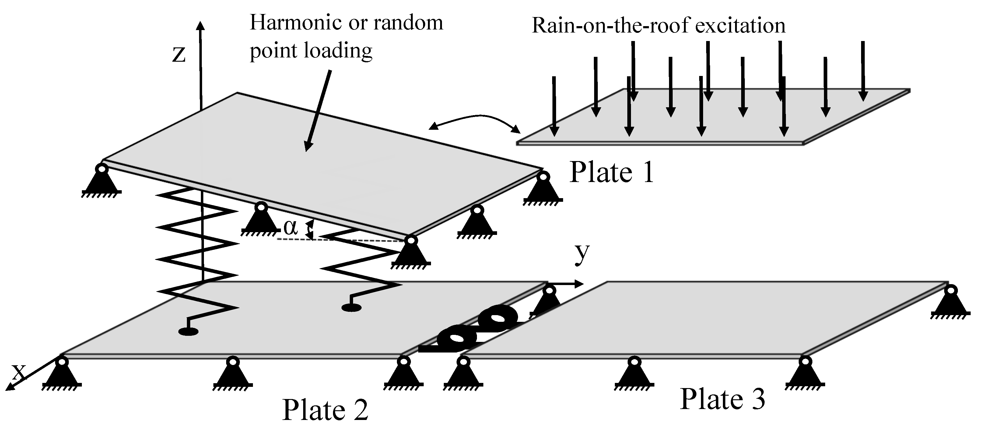
In fact, the traditional SEA assumes that the external input is the rain-on-the-roof type, which is a both spatial- and tempo-uncorrelated distributed loading. This assumption is consistent with many engineering applications, e.g., those which involve fluid-structure interaction loading-type affected by randomness. Therefore, actual difficulties occur when the dynamic system, modelled through hybrid FE-SEA, includes nonlinearities. The linearised FE-SEA formulation for the harmonic loading has already been derived in a previous authors’ work [21]; thus, the present investigations will further focus on the energy response of nonlinear dynamic systems subjected to random loading. More specifically, nonlinear dynamic systems with localized cubic nonlinearities introduced by translational and torsional springs, as joint components, are taken into account. Both harmonic and random loading-types are considered, and both point or distributed loadings are applied. The response of the dynamic systems was examined in terms of ensemble average of the time-averaged energy.

2. Benchmark Model-Lagrange-Rayleigh-Ritz Method

This section is entirely devoted to the derivation of the governing equations (GEs) for the benchmark model. The latter is used in all of the proposed case studies for validation purpose. The GEs are based on Kirchhoff’s thin-plate theory, the LRRM is performed to solve the linearised GEs. Various scenarios accounting for inclined plates and nonlinear translational and rotational springs, as well as several loading-types, are considered. With respect to the solution of the nonlinear GEs, the MHB and the SL are employed as linearisation techniques for systems excited by harmonic and random loadings, respectively. Some further information can be found in a previous article [19].

2.1. Built-Up System with Inclined Plate

The built-up system, schematically shown in Figure 1, is excited by an harmonic force P orthogonal to the inclined plate. The two plates are considered simply-supported, and the plate on top is inclined to an angle $\alpha$ with respect to the plate at the bottom. In the system, the out-of-plane motion is only considered. The stretch/compression of the translational spring can be written as $\Delta L_s=w_{1}cos\left(\alpha \right)-w_2$; where $w_1$ and $w_2$ denote the transverse displacement of plate 1 and plate 2, respectively. Then, the elastic potential energy of the built-up plate system, is given as:

$$\begin{array}{cc}\hfill & {\Phi }_e=\frac{1}{2}\sum _{mn}^{}{\omega }_{1,mn}^2{q}_{1,mn}^2+\frac{1}{2}\sum _{mn}^{}{\omega }_{2,mn}^2{q}_{2,mn}^2\hfill \\ \hfill & +\sum _{n_s=1}^{Ns}\frac{1}{2}{k}_{1,n_s}{\left[cos\left(\alpha \right)\sum _{mn}^{}{\psi }_{1,mn}\left({\mathbf{x}}_{k_s}\right)q_{1,mn}-\sum _{ij}^{}{\psi }_{2,ij}\left({\mathbf{x}}_{k_s}\right)q_{2,ij}\right]}^2\hfill \\ \hfill & +\sum _{n_s=1}^{Ns}\frac{1}{4}{k}_{3,n_s}{\left[cos\left(\alpha \right)\sum _{mn}^{}{\psi }_{1,mn}\left({\mathbf{x}}_{k_s}\right)q_{1,mn}-\sum _{ij}^{}{\psi }_{2,ij}\left({\mathbf{x}}_{k_s}\right)q_{2,ij}\right]}^4\hfill \end{array}.$$

(1)

The kinetic energy of the system, including the randomly distributed masses on the plates, is given as follows:

$$\begin{array}{cc}\hfill & T=\frac{1}{2}\sum _{mn}^{}{\dot{q}}_{1,mn}^2+\sum _{k=1}^{N_{1,m}}\frac{m_k}{2}\sum _{mn}^{}\sum _{ij}^{}{\dot{q}}_{1,mn}^2{\dot{q}}_{1,ij}^2{\psi }_{1,mn}\left({\mathbf{x}}_{m_k}\right){\psi }_{1,ij}\left({\mathbf{x}}_{m_k}\right)\hfill \\ \hfill & +\frac{1}{2}\sum _{mn}^{}{\dot{q}}_{2,mn}^2+\sum _{k=1}^{N_{2,m}}\frac{m_k}{2}\sum _{mn}^{}\sum _{ij}^{}{\dot{q}}_{2,mn}^2{\dot{q}}_{2,ij}^2{\psi }_{2,mn}\left({\mathbf{x}}_{m_k}\right){\psi }_{2,ij}\left({\mathbf{x}}_{m_k}\right)\hfill \end{array}.$$

(2)

The potential energy related to the application of the external force assumed to be concentrated and perpendicular to the upper plate can be written as

$${\Phi }_{ext}={\widehat{P}}_1\left(t\right)\left[\sum _{mn}^{}{\psi }_{1,mn}\left({\mathbf{x}}_{P_1}\right)q_{1,mn}\right].$$

(3)

It should be noted that, in addition to the random and harmonic point loadings, both rain-on-the-roof and harmonically distributed loading-types are taken into account in the present investigation. By using the Lagrange equations,

$$\frac{\mathrm{d}}{\mathrm{d}t}\left(\frac{\partial T}{\partial {\dot{q}}_{mn}}\right)-\frac{\partial T}{\partial q_{mn}}+\frac{\partial {\Phi }_e}{\partial q_{mn}}=\frac{\partial {\Phi }_{ext}}{\partial q_{mn}},$$

(4)

the GEs for a built-up plate system with nonlinear springs, inclination angle end harmonic point loading can be written as

$$\begin{array}{cc}\hfill & {\ddot{q}}_{1,mn}+{\omega }_{1,mn}^2{q}_{1,mn}+\sum _{k=1}^{N_{1,m}}{m}_k\sum _{ij}^{}{\ddot{q}}_{1,ij}{\psi }_{1,ij}\left({\mathbf{x}}_{m_k}\right){\psi }_{1,mn}\left({\mathbf{x}}_{m_k}\right)\hfill \\ \hfill & +\sum _{ns=1}^{Ns}{k}_{1,n_s}\left[cos\left(\alpha \right)\sum _{ij}^{}{q}_{1,ij}{\psi }_{1,ij}\left({\mathbf{x}}_{n_s}\right)-\sum _{ij}^{}{q}_{2,ij}{\psi }_{2,ij}\left({\mathbf{x}}_{n_s}\right)\right]cos\left(\alpha \right){\psi }_{1,mn}\left({\mathbf{x}}_{n_s}\right)\hfill \end{array}$$

(5)

$$\begin{array}{cc}\hfill & +\sum _{ns=1}^{Ns}{k}_{3,n_s}{\left[cos\left(\alpha \right)\sum _{ij}^{}{q}_{1,ij}{\psi }_{1,ij}\left({\mathbf{x}}_{n_s}\right)-\sum _{ij}^{}{q}_{2,ij}{\psi }_{2,ij}\left({\mathbf{x}}_{n_s}\right)\right]}^{3}cos\left(\alpha \right){\psi }_{1,mn}\left({\mathbf{x}}_{n_s}\right)\hfill \\ \hfill & ={\widehat{P}}_1{\psi }_{1,mn}\left({\mathbf{x}}_{P_1}\right)sin(\omega t+\varphi ),\hfill \\ \hfill \\ \hfill & {\ddot{q}}_{2,mn}+{\omega }_{2,mn}^2{q}_{2,mn}+\sum _{k=1}^{N_{2,m}}{m}_k\sum _{ij}^{}{\ddot{q}}_{2,ij}{\psi }_{2,ij}\left({\mathbf{x}}_{m_k}\right){\psi }_{2,mn}\left({\mathbf{x}}_{m_k}\right)\hfill \\ \hfill & +\sum _{ns=1}^{Ns}{k}_{1,n_s}\left[\sum _{ij}^{}{q}_{2,ij}{\psi }_{2,ij}\left({\mathbf{x}}_{n_s}\right)-cos\left(\alpha \right)\sum _{ij}^{}{q}_{1,ij}{\psi }_{1,ij}\left({\mathbf{x}}_{n_s}\right)\right]{\psi }_{2,mn}\left({\mathbf{x}}_{n_s}\right)\hfill \\ \hfill & +\sum _{ns=1}^{Ns}{k}_{3,n_s}{\left[\sum _{ij}^{}{q}_{2,ij}{\psi }_{2,ij}\left({\mathbf{x}}_{n_s}\right)-cos\left(\alpha \right)\sum _{ij}^{}{q}_{1,ij}{\psi }_{1,ij}\left({\mathbf{x}}_{n_s}\right)\right]}^3{\psi }_{2,mn}\left({\mathbf{x}}_{n_s}\right)\hfill \\ \hfill & =0.\hfill \end{array}$$

(6)

In Equations (5) and (6), $q_{mn}$ are the time-dependent modal coordinates; ${\psi }_{mn}$ are the mass-normalized shape functions; m and n represent the Ritz expansion order in the x and y direction, respectively; $N_1,m$ and $N_2,m$ are the number of the distributed lumped masses used to randomize plate 1 and plate 2, respectively; $k_1$ and $k_3$ are the linear and nonlinear stiffness coefficients of the connection springs; and $N_s$ refers to the number of springs introduced as joint elements amongst subsystems.

2.2. Random Loading and Statistical Linearization

Consider the situation schematically shown in Figure 1 with the random loading acting on plate 1 but its inclination angle is equal to zero ($\alpha =0$). The external force is vertically downward and concentrated, assumed to be white noise with mean value ${\mu }_P$ and standard deviation ${\sigma }_P$. The linearised equations of motion can be written as

$${\mathbf{M}}_0\ddot{\mathbf{q}}+{\mathbf{C}}_0\dot{\mathbf{q}}+{\mathbf{K}}_{eq}\mathbf{q}=\mathbf{P},$$

(7)

where ${\mathbf{M}}_0$ and ${\mathbf{C}}_0$ are mass and damping matrices; $\mathbf{q}$ is the generalized displacement; $\mathbf{P}$ represents generalized force; ${\mathbf{K}}_{eq}$ is the equivalent stiffness matrix. To solve the above equations, the calculation of the equivalent stiffness is fundamental. In this respect, the SL can be successfully used.

With respect to the single-degree system, described by the differential equation $m\ddot{x}+c\dot{x}+k_{1}x+k_3{x}^3=F$, where m, c, k denote the mass, damping, and stiffness of this system; x is the displacement; and the external force F follows normal distribution $F\sim N(\mu ,{\sigma }^2)$, statistical linearisation can be performed and the equation is transformed as $m\ddot{x}+c\dot{x}+k_{eq}x=F$, where

$$k_{eq}=k_1+3k_3〈x^2〉.$$

(8)

$k_{eq}$ is referred as equivalent stiffness; $〈x^2〉$ denotes the expectation of $x^2$ [23].

For the built-up system in Figure 1, the stretch or the compression of the translational spring Δ can be given as

$$\Delta =\sum _{mn}{\psi }_{1,mn}\left({\mathbf{x}}_s\right)q_{1,mn}-\sum _{ij}{\psi }_{2,ij}\left({\mathbf{x}}_s\right)q_{2,ij};$$

(9)

thence,

$$\begin{array}{cc}\hfill 〈{\Delta }^2〉& =〈{\left(\sum _{mn}{\psi }_{1,mn}\left({\mathbf{x}}_s\right)q_{1,mn}\right)}^2〉+〈{\left(\sum _{ij}{\psi }_{2,ij}\left({\mathbf{x}}_s\right)q_{2,ij}\right)}^2〉\hfill \\ \hfill & -2〈\left(\sum _{mn}{\psi }_{1,mn}\left({\mathbf{x}}_s\right)q_{1,mn}\right)\left(\sum _{ij}{\psi }_{2,ij}\left({\mathbf{x}}_s\right)q_{2,ij}\right)〉\hfill \\ \hfill & =\sum _{mn}\sum _{ij}{\psi }_{1,mn}\left({\mathbf{x}}_s\right){\psi }_{1,ij}\left({\mathbf{x}}_s\right)〈q_{1,mn}{q}_{1,ij}〉\hfill \\ \hfill & +\sum _{mn}\sum _{ij}{\psi }_{2,mn}\left({\mathbf{x}}_s\right){\psi }_{2,ij}\left({\mathbf{x}}_s\right)〈q_{2,mn}{q}_{2,ij}〉\hfill \\ \hfill & -2\sum _{mn}\sum _{ij}{\psi }_{1,mn}\left({\mathbf{x}}_s\right){\psi }_{2,ij}\left({\mathbf{x}}_s\right)〈q_{1,mn}{q}_{2,ij}〉.\hfill \end{array}$$

(10)

It should be born in mind that the linearised stiffness matrix derived by using MHB and SL, and considering a cubic nonlinearity, are different. For the former, it can be written as $k_{eq}=k_1+\frac{3}{4}{k}_3{x}^2$, while, for the latter, it is given in Equation (8). In addition, since Equation (7) is in time domain, it is necessary to obtain the energy in a time-averaged form (see Ref. [19]).

3. The Linearized Hybrid FE-SEA Formulation

The present section provides a overview of the hybrid FE-SEA formulation accounting for nonlinearities in the point joints of dynamic system. The hybrid FE-SEA formulation firstly requires the identification of those components, within the system, which are assumed to behave statistically. These components are modelled as SEA subsystems. The remaining components are deemed to be deterministic and are modelled by FE method. The relationship between the SEA and the FE subsystems is considered to satisfy the following conditions [5]:

$${\mathbf{D}}_{tot}\mathbf{q}=\mathbf{f}+\sum _k^{}{\mathbf{f}}_{rev}^k,$$

(11)

$${\mathbf{D}}_{tot}={\mathbf{D}}_d+\sum _k^{}{\mathbf{D}}_{dir}^k,$$

(12)

where $\mathbf{q}$ is the general displacement vector of FE parts under the frequency of $\omega$; $\mathbf{f}$ represents the external forces vector exerted to the FE components; ${\mathbf{f}}_{rev}^k$ is the forces vector resulting from the reverberant field in k-th subsystem; ${\mathbf{D}}_d$ corresponds to the dynamic stiffness matrix of the deterministic components; and ${\mathbf{D}}_{dir}^k$ is the the dynamic stiffness matrix arising from k-th direct field. Considering the diffuse field reciprocity relation between direct fields and reverberant fields [6], the energy equilibrium equation for each subsystem and the cross spectral matrix ${\mathbf{S}}_{qq}$ is given as [5]:

$$\omega \left({\eta }_j+{\eta }_{d,j}\right)+\sum _k^{}\omega {\eta }_{jk}{n}_j\left(\frac{E_j}{n_j}-\frac{E_k}{n_k}\right)=P_{in,j}+P_{in,j}^{ext},$$

(13)

$${\mathbf{S}}_{qq}={\mathbf{D}}_{tot}^{-1}\left[{\mathbf{S}}_{ff}+\sum _k\left(\frac{4E_k}{\omega \pi n_k}\right)\mathrm{Im}\left\{{\mathbf{D}}_{dir}^{\left(k\right)}\right\}\right]{\left({\mathbf{D}}_{tot}^{-1}\right)}^{*T},$$

(14)

where

$$\begin{array}{c}\hfill P_{in,j}^{ext}=\left(\frac{\omega }{2}\right)\sum _{rs}\mathrm{Im}\left\{D_{dir,rs}^j\right\}{\left[{\mathbf{D}}_{tot}^{-1}{\mathbf{S}}_{ff}{\left({\mathbf{D}}_{tot}^{-1}\right)}^{*T}\right]}_{rs},\end{array}$$

(15)

$${\eta }_{jk}=\frac{2}{\omega \pi n_j}\sum _{rs}\mathrm{Im}\left\{D_{dir,rs}^j\right\}{\left[{\mathbf{D}}_{tot}^{-1}\mathrm{Im}\left\{{\mathbf{D}}_{dir}^{\left(k\right)}\right\}{\left({\mathbf{D}}_{tot}^{-1}\right)}^{*T}\right]}_{rs},$$

(16)

$${\eta }_{d,j}=\frac{2}{\omega \pi n_j}\sum _{rs}\mathrm{Im}\left\{D_{d,rs}\right\}{\left[{\mathbf{D}}_{tot}^{-1}\mathrm{Im}\left\{{\mathbf{D}}_{dir}^{\left(j\right)}\right\}{\left({\mathbf{D}}_{tot}^{-1}\right)}^{*T}\right]}_{rs}.$$

(17)

In Equation (13), ${\eta }_j$ is the loss factor of j-th subsystem; ${\eta }_{d,j}$ corresponds to the power dissipation in j-th master system; ${\eta }_{jk}$ is the coupling loss factor; $n_j$ is the modal density; $E_j$ is the ensemble average energy of j-th subsystem; $P_{in,j}$ and $P_{in,j}^{ext}$ represent the power input from the loadings to subsystems and to master systems, respectively. In Equation (14), ${\mathbf{S}}_{ff}$ denotes the cross spectral matrix of external forces to master systems. Usually, Equations (13) and (14) are used to obtain the response of subsystems and FE components. To solve Equation (13), $P_{in,j}^{ext}$, ${\eta }_{jk}$ and ${\eta }_{d,j}$ can be calculated by Equations (15)–(17). Then, the responses of deterministic components are obtained using Equation (14). As far as the localized nonlinearity is concerned, it is treated exactly in the same way of the LRRM benchmark model. In the previous authors’ article [19], it is illustrated the linearisation of the MHB corresponding to harmonic loading; this section similarly applies the SL for the localized cubic nonlinearities (translational and/or torsional springs) under random loading.

4. Numerical Results

This section provides both validation and assessment of the linearised hybrid FE-SEA formulation regarding to both harmonic and random excitations. Three case studies are addressed; the first case study is made up of a three-plate build-up system accounts for both harmonic and random point loadings, rain-on-the-roof loading-type and inclination angle of the driven plate; the second case study focuses on the harmonically distributed excitation on a four-plate dynamic system; the third case study investigates a different four-plate dynamic system loaded by a white noise random point loading. The case study is based on the simulation of built-up plate systems with linear and nonlinear translational and/or torsional springs. In all of the addressed case studies, the thin plate is homogeneous, isotropic, and linear elastic with Young’s modulus $E=70$ GPa; Poisson’s ratio $\nu =0.3$; and density $\rho =2700$ kg/m³. The plates’ damping loss factors, modal densities, and sizes, including a and b (plate’s sides), as well as h (thickness), are given in the

Table 1. Plate parameters.

Plate	Edge a (m)	Edge b (m)	Thickness (mm)	Loss Factor $\mathit{\eta }$	Modal Density (Modes/Hz)
1	1.35	1.2	5	0.01	0.0942
2	1.05	1.2	15	0.01	0.0245
3	1.05	1.2	5	0.01	0.0733
4	1.35	1.2	5	0.03	0.0942

. The linear and nonlinear translational spring elastic coefficients are given as $k_l=2\times {10}^5$ and $k_{nl}=2\times {10}^{15}$, respectively. Those for torsional spring are given as $k_{\theta l}={10}^3$ and $k_{\theta nl}={10}^{12}$. With regard to the LRRM+MCS, the lumped masses are used to break the system symmetries inducing the Gaussian Orthogonal Ensemble (GOE) [21,33]. This paper applies 20 masses with 2.0% mass rate to the bare plate according to the authors’ previous paper [21]. Besides, 50 Monte Carlo samples are utilized to calculate the ensemble average energy response.

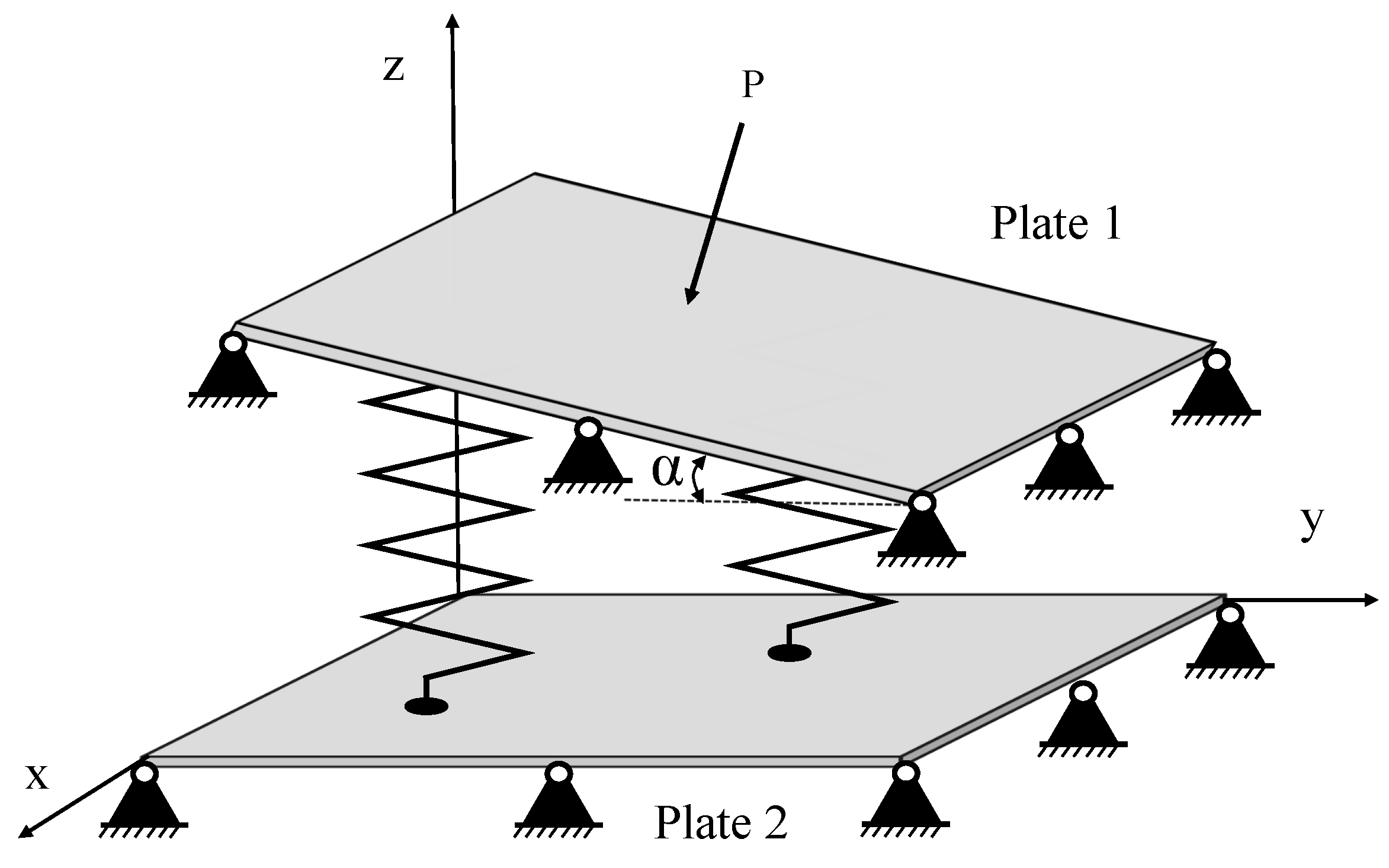
4.1. Case Study 1: Harmonic and Random Point-Load Excitations, as Well as Rain-on-the-Roof Loading

The schematic figure of first case study is shown in Figure 2. It includes three plates one of which is an with inclined angle $\alpha$ and excited by various loading types perpendicular to plate 1 middle surface. We consider several situations for this case studies for the purpose of finding what factors could effect the energy response of each subsystem within the built-up system. In the first situation, we explore the energy cascade through subsystem by changing the inclination angles. The translational springs are set to be nonlinear, while the torsional ones are linear. Different inclination angles, e.g., $0^{\circ }$, ${30}^{\circ }$, ${60}^{\circ }$, and ${80}^{\circ }$, are applied to plate 1, the external excitation applied to plate 1 is considered to be an harmonic point load. 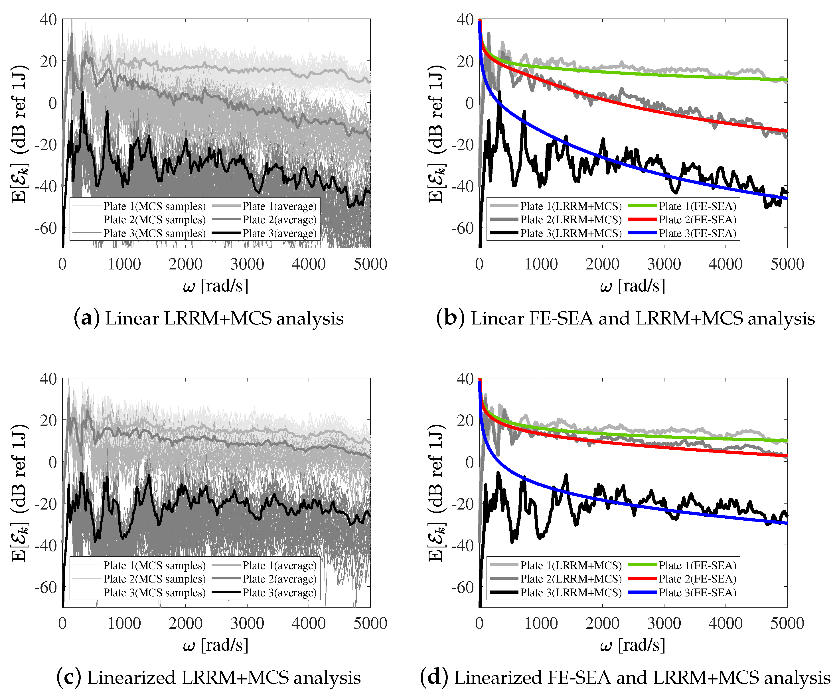Figure 3 depicts the ensemble average energy for both linear and linearised FE-SEA and LRRM+MCS analysis with $\alpha =0$. In the figure, the average energy of LRRM+MCS analysis fluctuates dramatically in lower-frequency range but tends to keep stable and close to the response obtained by using the hybrid FE-SEA formulation in higher-frequency range. This is because lower-frequency modes are hard to be randomized by uncertainties, due to the fact that the energy response in low-frequency range is mainly influenced by resonant modes. The higher-frequency modes are, instead, more affected by the randomization induced by the lumped masses, which leads to the mixing and veering of the modes and then to the Rayleigh distribution. It is noted that the energy responses obtained via LRRM+MCS analysis compare well with those computed through the hybrid FE-SEA method for both linear and linearised formulation. 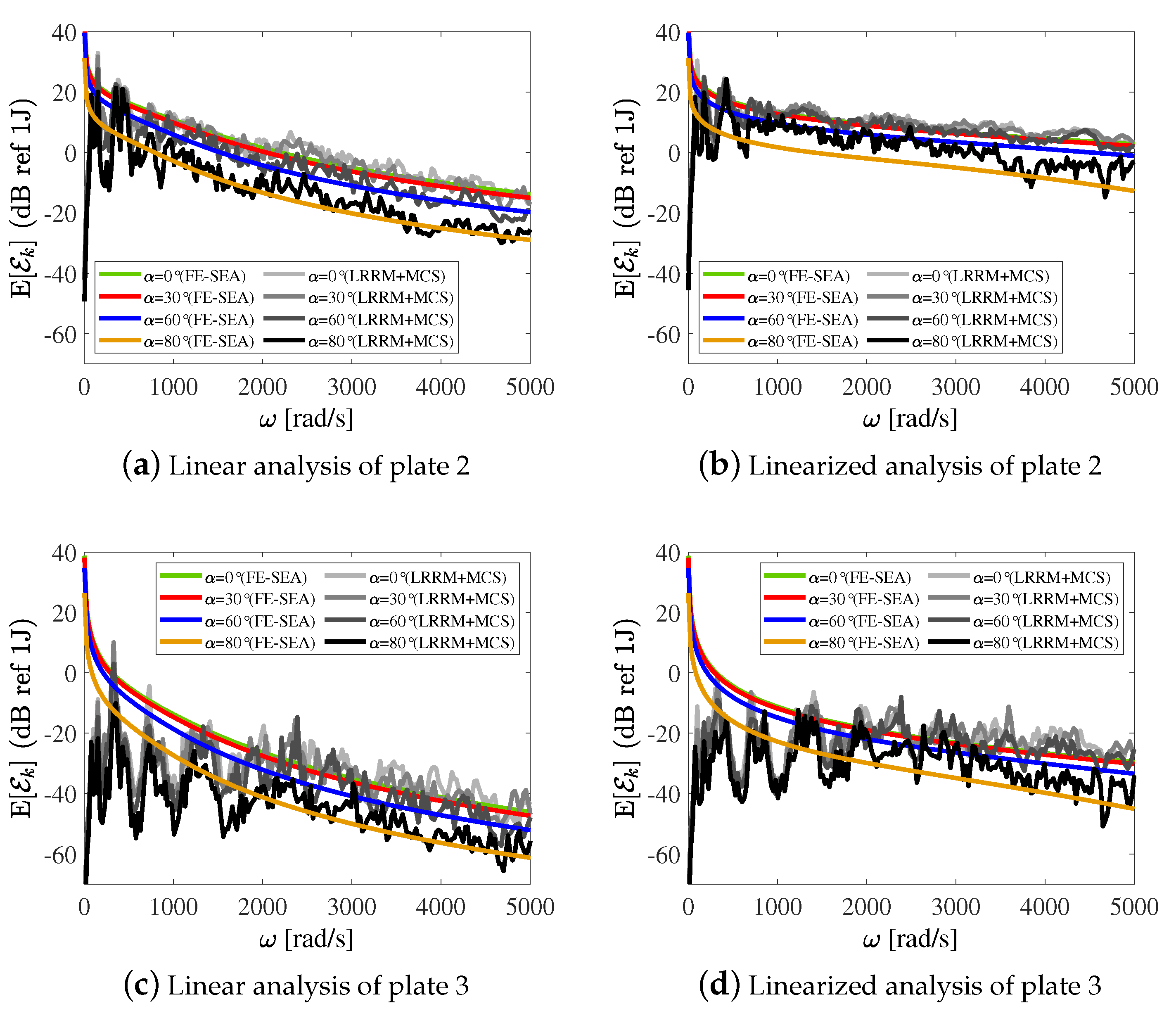This can also be seen in Figure 4, which shows the linear and linearised FE-SEA and LRRM+MCS analysis of plate 2 and plate 3 at different inclination angles. In this figure, it should be noted that, when the angle varies from $0^{\circ }$ to ${30}^{\circ }$, the average energy response just slightly decreases, whilst, from ${60}^{\circ }$ to ${80}^{\circ }$, a significant reduction is observed.

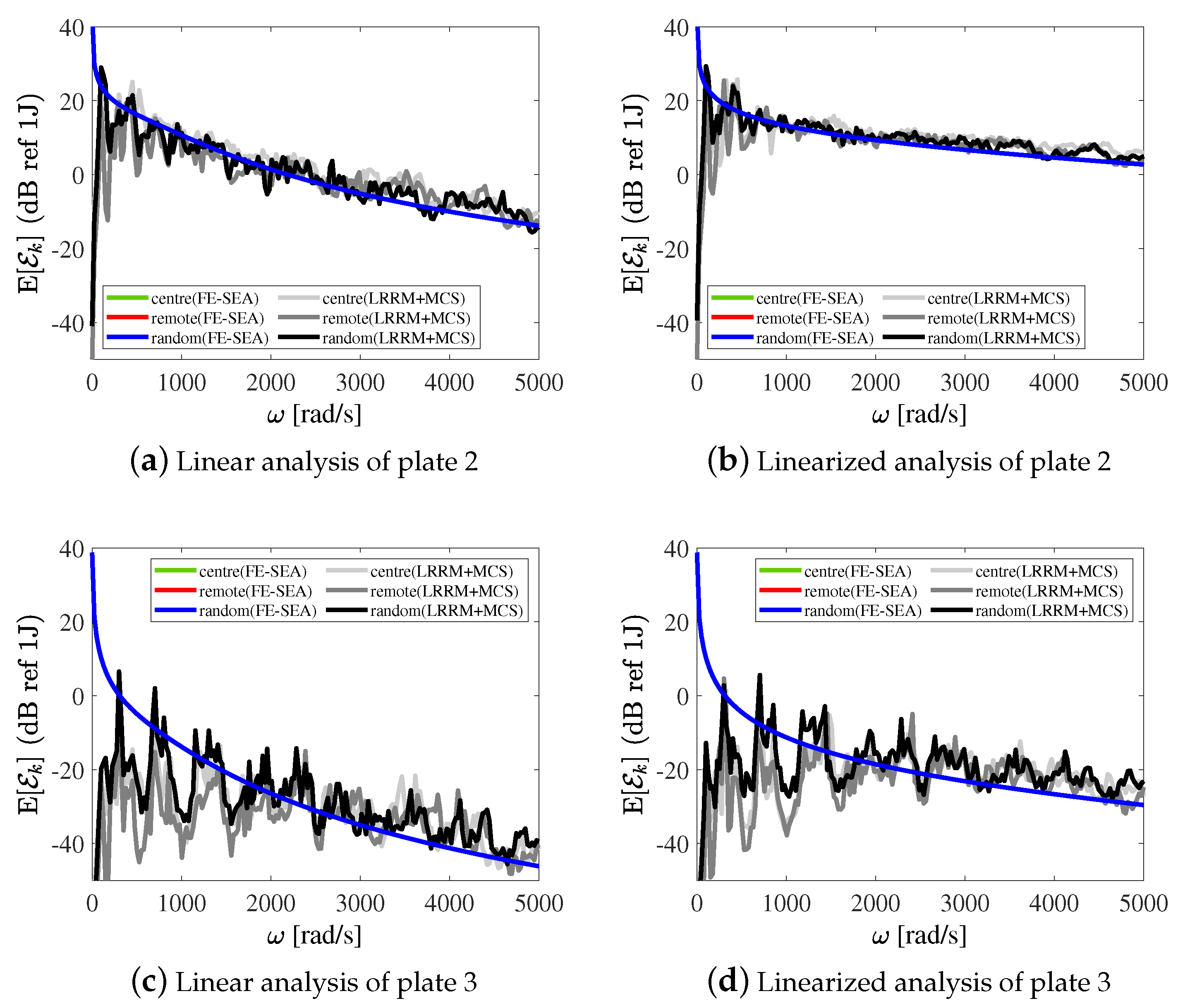
The second scenario of the first case study explores the influence by the spring position. The inclination angle is set to be zero, and the translational springs are linear and torsional springs are nonlinear. Three conditions in the spring position are considered: (i) the centre of plate 1 [coordinate (0.5a,0.5b)]; (ii) a remote position from the centre [coordinate (0.05a, 0.5b)]; and (iii) a random position in every MCS sample. The loading is still set as the harmonic point excitation. Results are shown in Figure 5 for both linear and linearised FE-SEA and LRRM+MCS analysis. As expected, all the energy responses calculated by means of the hybrid FE-SEA approach do not change prominently. This is because the FE-SEA method randomizes the spring position and estimates the average results; in other words, no specific positions of the joints are required. It can also be noted an excellent match between the linearised FE-SEA formulation and the benchmark model.

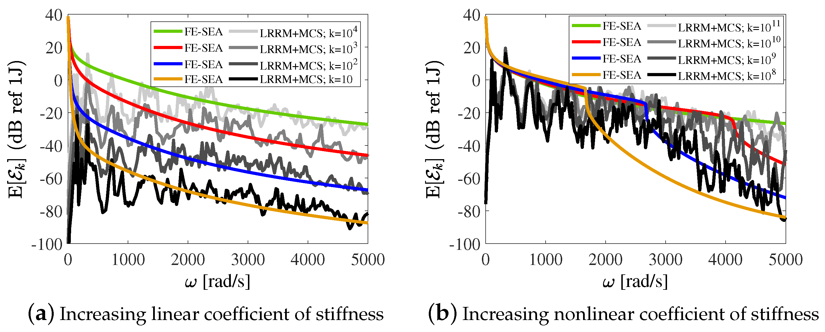
Next, investigation within the case study 1 considers different values of the springs stiffness coefficients. As the exploration to translational spring stiffness coefficients has been made in the previous work [21], this investigation focus on the torsional spring. We separately increase the linear and nonlinear stiffness coefficients of the torsional springs, while keeping the harmonic point loading as external excitation. Figure 6a is obtained by increasing the linear coefficients from 10 to ${10}^2$, ${10}^3$, and ${10}^4$, respectively. The energy response by linearised FE-SEA which matches the benchmark model increases very smoothly with the rise of linear coefficients. In Figure 6b, the increase of the nonlinear stiffness coefficient from ${10}^8$ to ${10}^9$, ${10}^{10}$, and ${10}^{11}$ generates an energy level rise in different frequency range. Smaller nonlinear stiffness coefficient values influence the energy level in lower-frequency range, while the larger ones effect the higher-frequency range. A similar trend was obtained in a previous work for focused on translational springs [21].

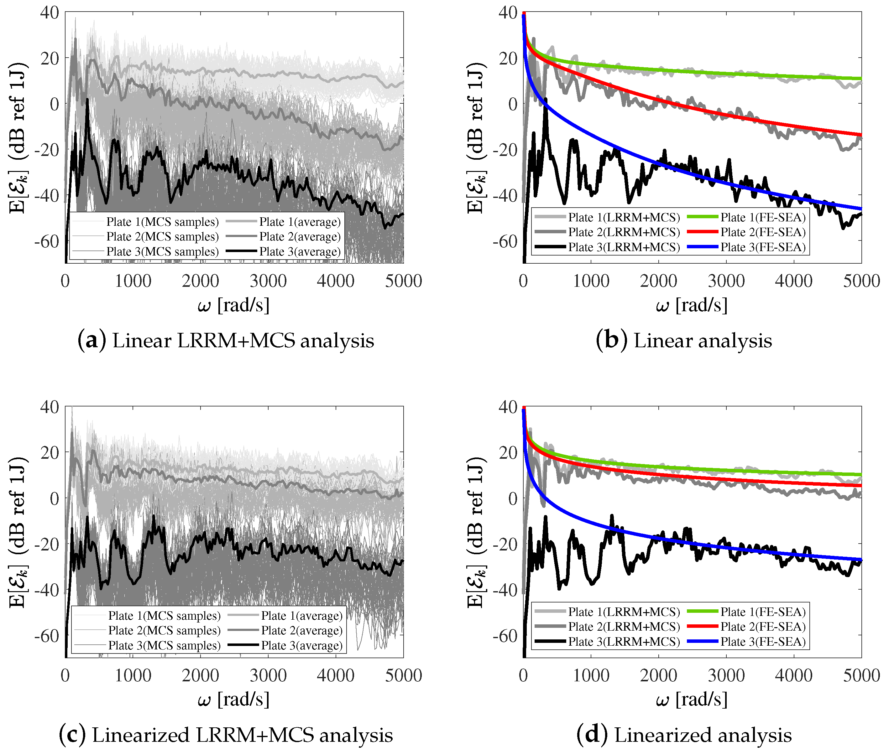
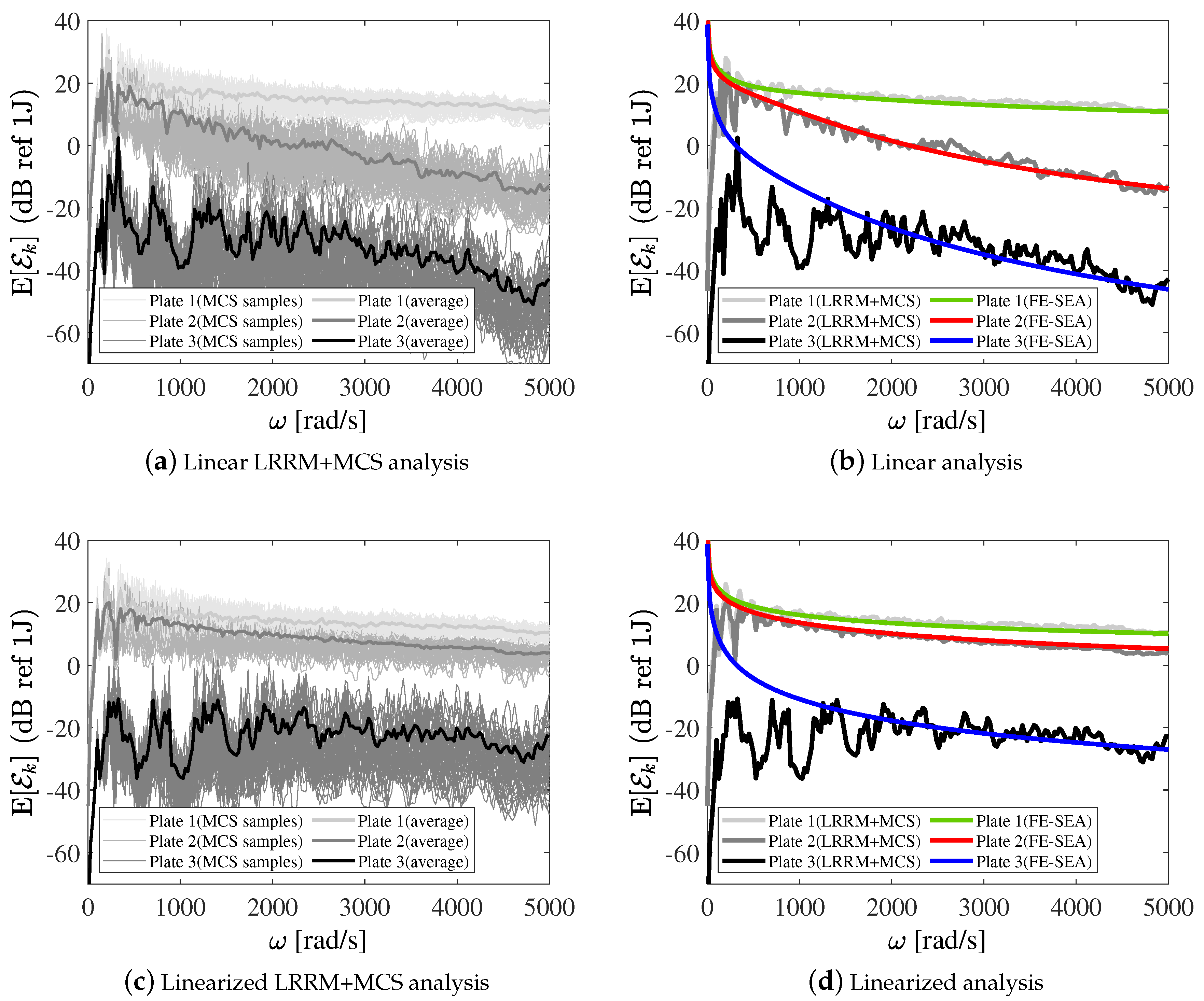
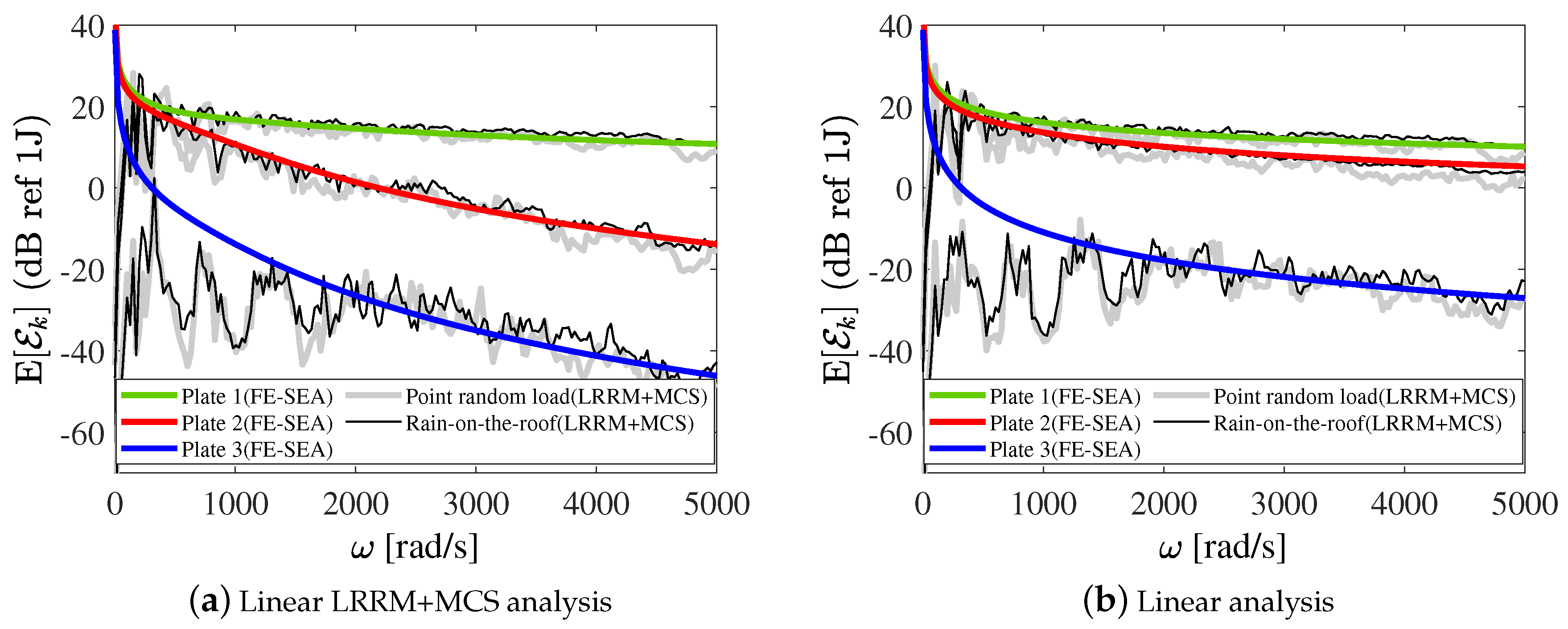
The built-up system in Figure 2 is now considered to be excited by a white noise loading on plate 1. The statistical linearisation is the one used to derive the linearised FE-SEA formulation. For the white noise point excitation, Figure 7 presents both the linear and the linearised results computed by using both the hybrid FE-SEA method and the benchmark model. A good match can be seen between two different analyses. We also considered another situation: rain-on-the-roof excitation on plate 1. The energy responses can be found in Figure 8. Besides the good agreement between the linearised hybrid FE-SEA model and LRRM+MCS formulation, the results yielded by the benchmark model are smoother than those with point random loading, and the MCS sample cloud of rain-on-the-roof is thinner than those of the point random load, due to that fact that rain-on-the-roof is evenly distributed on the surface of the plate, and it can help realize better randomization for the modes.

In Figure 9, the system energy responses with both point random load and rain-on-the-roof as external excitations for both linear and linearised hybrid FE-SEA formulation are depicted. It can be noted that the energy level of plate 2 around 4000 rad/s excited by rain-on-the-roof remains steady, while those evaluated by using the point random load show some oscillations.

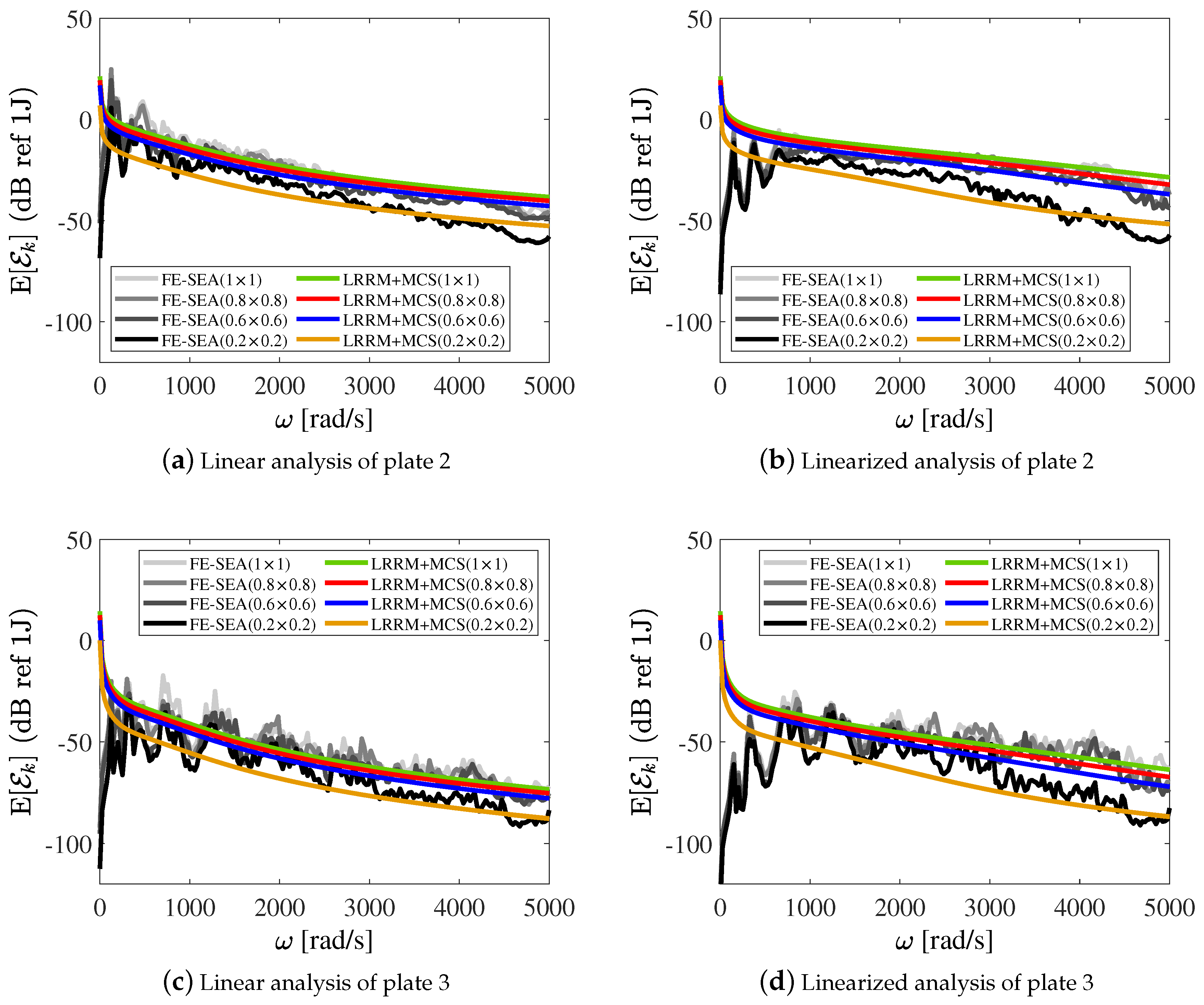
4.2. Case Study 2: Distributed Loading

This case study focuses on the harmonic distributed loading on the built-up plate system. The four-plate system with both translational and torsional springs, schematically shown in Figure 10, with localized nonlinearity in the spring set 1, is investigated. The distributed loading is set to excite plate 1 orthogonally to the middle surface. Different loading areas are applied in order to explore its effects on the energy response. The loading area varies from the small value of $0.2\times 0.2$ to the larger of $0.6\times 0.6$, $0.8\times 0.8$, $1\times 1$, where the case $1\times 1$ means that the distributed harmonic load area equals the plate surface. The average energy responses related to this latest case are depicted in Figure 11. The energy response of the linearised analysis increases comparing to those of linear analysis for the reason of cubic harden stiffness. In Figure 12, energy response of plate 2 and plate 3 for different loading area on plate 1 is shown. It can be observed that a larger gap between the energy responses with loading area $0.2\times 0.2$ and $0.6\times 0.6$ occurs.

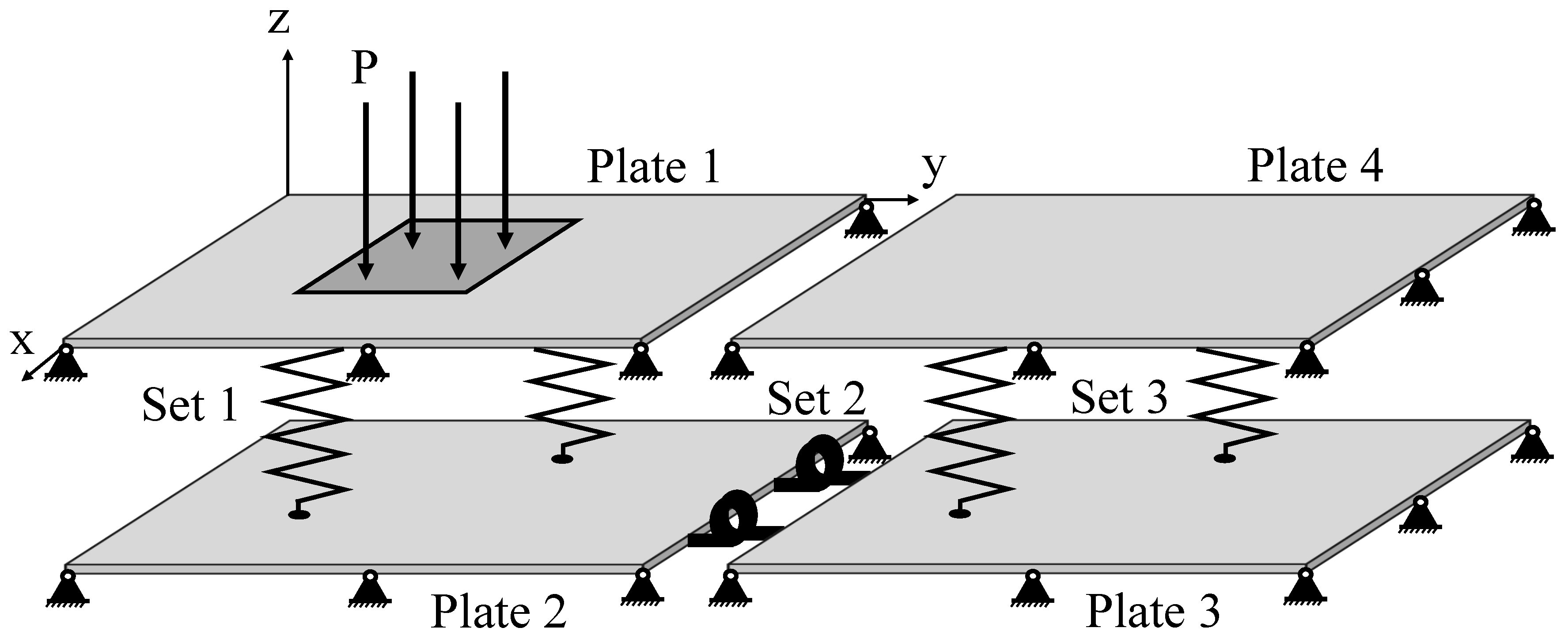
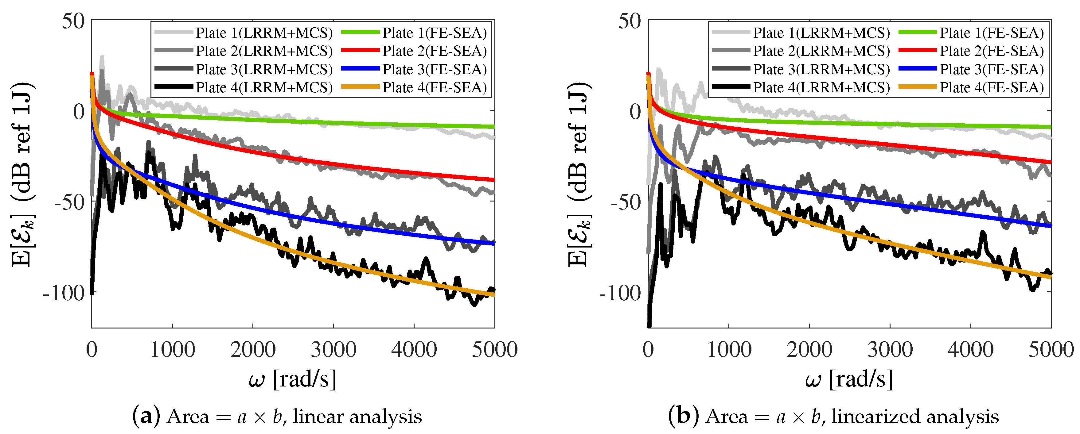
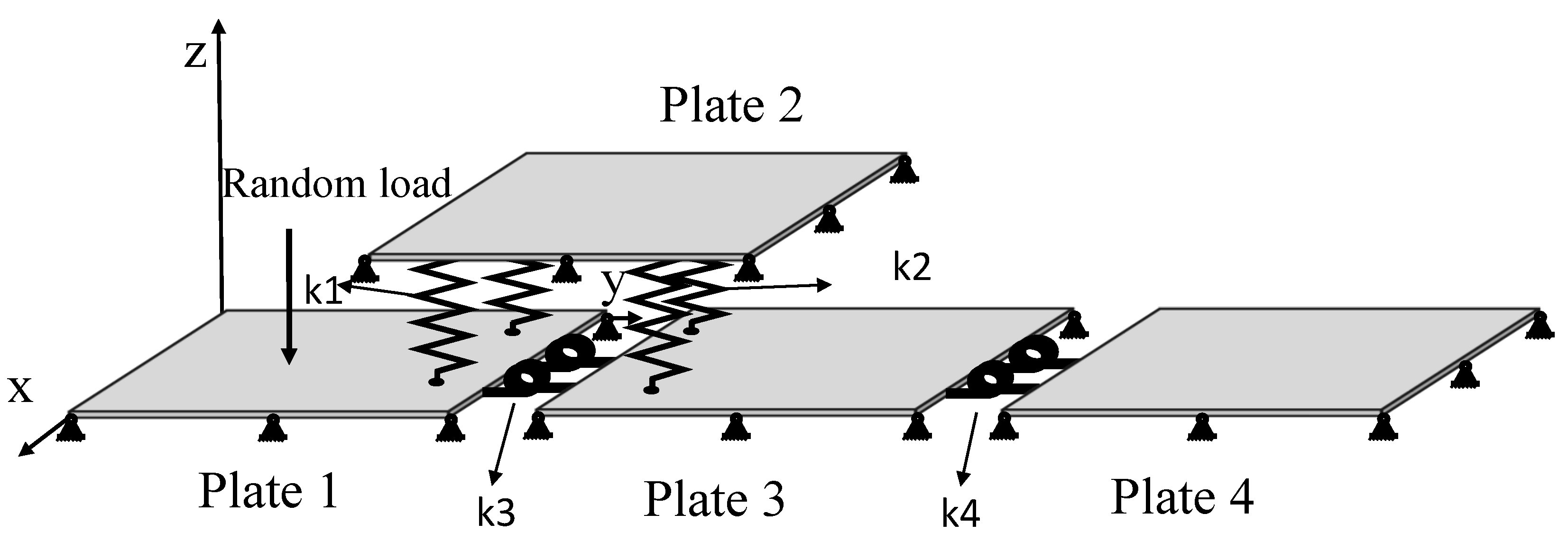
4.3. Case Study 3: Four-Plate Built-Up System

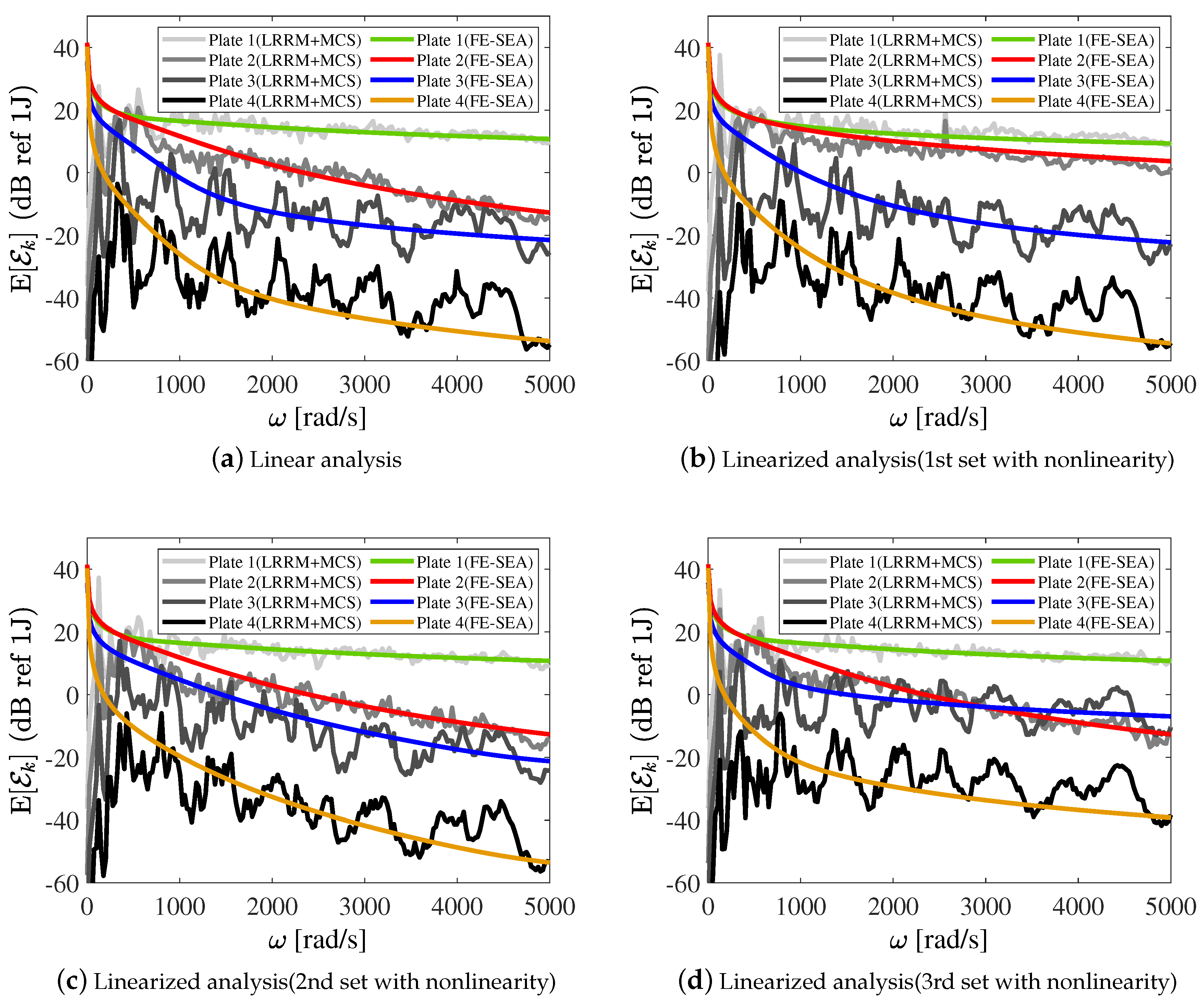
To further test the linearised FE-SEA formulation towards random loading, a more complex case study consisting of four-plate built-up system, shown in Figure 13, is addressed. All the plate parameters can be found in Table 1. The white noise point load in the figure orthogonally excites plate 1. Four cases are considered: (i) all spring sets are linear; (ii) only the first spring set is nonlinear; (iii) only the second spring set contains nonlinearity; (iv) only the third spring set is nonlinear. The energy responses from both linear and linearised FE-SEA and LRRM+MCS analysis are shown in Figure 14. Comparing the linear energy response given in Figure 14a with those of the second case shown in Figure 14b, the energy response of plate 2 significantly increases as the nonlinearity is applied, while those of the other plate subsystems are only slightly affected. A very similar result can be observed by comparing Figure 14a with Figure 14c, where only the energy level of plate 3 ramps up significantly due to the nonlinearity in second spring set. However, the nonlinearity existing in third spring set changes the energy response in a very different manner with respect to the previous two cases. Figure 14d demonstrates that: (1) the energy level of both plate 3 and 4 steps up remarkably due to the nonlinearity; (2) a cross of the curve of energy level of plate 2 and plate 3 can occur. Moreover, an excellent match between linear and linearised FE-SEA method and LRRM+MCS analysis is presented in all the faced cases.

5. Conclusions

The present article proposes a linearised hybrid FE-SEA formulation for the dynamic response of build-up systems featured by nonlinear joints and subjected to both harmonic and random excitations. The formulation was validated by developing a benchmark model based on the combination of both the Lagrange-Rayleigh-Ritz method and the Monte Carlo Simulation technique. Within the framework of the benchmark model, each plate subsystem of the dynamic system is modelled by using Kirchhoff’s thin plate theory. The two different linearisation procedures are used according to the external excitation type. More specifically, in the case of harmonic excitation, the method of harmonic balance was employed; in the case of random excitation, the statistical linearisation was used. Various case studies were examined to both validate and assess the new hybrid FE-SEA formulation. From all the analyses carried out, the following main conclusions can been drawn:

• The plate inclination angle within the built-up systems slightly affects the energy response for small values; on the contrary, its effect tends to be prominent for inclination angle close to ${90}^{\circ }$.
• The springs’ position—acting as joint components—, as expected, does not affect the energy response.
• Larger values of the cubic nonlinear stiffness coefficients of the torsional springs increase the energy level in a wider frequency range affecting also the higher frequency.
• Comparing the random point load with the rain-on-the-roof excitation can realize better randomization from the perspective of the LRRM, namely the energy level of the rain-on-the-roof tends to be closer to that of FE-SEA formulation.
• The hybrid FE-SEA formulation is enormously less computationally expensive than the benchmark model based on MCS technique. (Computer specifications: Windows 10 Home, Intel(R) Core(TM) i5-8300H CPU @ 2.30GHz, 8.00 GB installed memory (RAM), 64-bit Operating System, x64-based processor.)
• In all of the addressed case studies, the MHB and the SL, employed in both the hybrid FE-SEA formulation and the benchmark model, turned out to be highly effective in the linearisation process of built-up systems with localized nonlinearity.

References

1. Lyon, R.H. Statistical Energy Analysis of Dynamical Systems: Theory and Applications; MIT Press: Cambridge, MA, USA, 1975. [Google Scholar]
2. Lyon, R.H.; DeJong, R.G.; Heckl, M. Theory and application of statistical energy analysis. J. Acoust. Soc. Am. 1995, 98, 3021. [Google Scholar] [CrossRef]
3. Hodges, C.H.; Woodhouse, J. Theories of noise and vibration transmission in complex structures. Rep. Prog. Phys. 1986, 49, 107. [Google Scholar] [CrossRef]
4. Langley, R.S.; Bremner, P. A hybrid method for the vibration analysis of complex structural-acoustic systems. J. Acoust. Soc. Am. 1999, 105, 1657–1671. [Google Scholar] [CrossRef]
5. Shorter, P.J.; Langley, R.S. Vibro-acoustic analysis of complex systems. J. Sound Vib. 2005, 288, 669–699. [Google Scholar] [CrossRef]
6. Shorter, P.J.; Langley, R.S. On the reciprocity relationship between direct field radiation and diffuse reverberant loading. J. Acoust. Soc. Am. 2005, 117, 85–95. [Google Scholar] [CrossRef]
7. Cotoni, V.; Shorter, P.; Langley, R.S. Numerical and experimental validation of a hybrid finite element-statistical energy analysis method. J. Acoust. Soc. Am. 2007, 122, 259–270. [Google Scholar] [CrossRef]
8. Cicirello, A.; Langley, R.S. The vibro-acoustic analysis of built-up systems using a hybrid method with parametric and non-parametric uncertainties. J. Sound Vib. 2013, 332, 2165–2178. [Google Scholar] [CrossRef]
9. Cicirello, A.; Langley, R.S. Efficient parametric uncertainty analysis within the hybrid Finite Element/Statistical Energy Analysis method. J. Sound Vib. 2014, 333, 1698–1717. [Google Scholar] [CrossRef]
10. Yin, H.; Yu, D.; Yin, S.; Xia, B. Fuzzy interval finite element/statistical energy analysis for mid-frequency analysis of built-up systems with mixed fuzzy and interval parameters. J. Sound Vib. 2016, 380, 192–212. [Google Scholar] [CrossRef]
11. Culla, A.; D’Ambrogio, W.; Fregolent, A. Parametric approaches for uncertainty propagation in SEA. Mech. Syst. Signal Process. 2011, 25, 193–204. [Google Scholar] [CrossRef]
12. Xu, M.; Qiu, Z.; Wang, X. Uncertainty propagation in SEA for structural–acoustic coupled systems with non-deterministic parameters. J. Sound Vib. 2014, 333, 3949–3965. [Google Scholar] [CrossRef]
13. Christen, J.L.; Ichchou, M.; Troclet, B.; Bareille, O.; Ouisse, M. Global sensitivity analysis and uncertainties in SEA models of vibroacoustic systems. Mech. Syst. Signal Process. 2017, 90, 365–377. [Google Scholar] [CrossRef]
14. Chen, Q.; Fei, Q.; Wu, S.; Li, Y. Statistical Energy Analysis for the Vibro-Acoustic System with Interval Parameters. J. Aircr. 2019, 56, 1869–1879. [Google Scholar] [CrossRef]
15. Chen, Q.; Fei, Q.; Wu, S.; Li, Y. Uncertainty propagation of the energy flow in vibro-acoustic system with fuzzy parameters. Aerosp. Sci. Technol. 2019, 94, 105367. [Google Scholar] [CrossRef]
16. Carcaterra, A. Thermodynamic temperature in linear and nonlinear Hamiltonian Systems. Int. J. Eng. Sci. 2014, 80, 189–208. [Google Scholar] [CrossRef]
17. Sotoudeh, Z. Entropy and Mixing Entropy for Weakly Nonlinear Mechanical Vibrating Systems. Entropy 2019, 21, 536. [Google Scholar] [CrossRef] [Green Version]
18. Spelman, G.M.; Langley, R.S. Statistical energy analysis of nonlinear vibrating systems. Philos. Trans. R. Soc. Math. Phys. Eng. Sci. 2015, 373, 20140403. [Google Scholar] [CrossRef] [Green Version]
19. Fazzolari, F.A.; Langley, R.S. The Statistical Energy Analysis of Systems with Nonlinear Joints. In Proceedings of the 24th International Congress on Sounds and Vibration, London, UK, 24–27 July 2017. [Google Scholar]
20. Fazzolari, F.A. A hybrid finite element-statistical energy analysis formulation accounting for nonlinearities. In Proceedings of the 13th International Conference on Computing Sstructures Technologies, Sitges, Spain, 4–6 September 2018. [Google Scholar]
21. Fazzolari, F.A.; Tan, P. A Hybrid Finite Element-Statistical Energy Analysis Approach to the Dynamic Response of Built-up Systems with Nonlinear Joints. J. Sound Vib. 2020, in press. [Google Scholar] [CrossRef]
22. Worden, K. Nonlinearity in Structural Dynamics: Detection, Identification and Modelling; CRC Press: Boca Raton, FL, USA, 2019. [Google Scholar]
23. Roberts, J.B.; Spanos, P.D. Random Vibration and Statistical Linearization; Courier Corporation: North Chelmsford, MA, USA, 2003. [Google Scholar]
24. Peppin, R.J. An Introduction to Random Vibrations, Spectral and Wavelet Analysis; Courier Corporation: North Chelmsford, MA, USA, 1994. [Google Scholar]
25. Crandall, S.H.; Mark, W.D. Random Vibration in Mechanical Systems; Academic Press: Cambridge, MA, USA, 2014. [Google Scholar]
26. Roberts, J.B.; Spanos, P.D. Stochastic averaging: An approximate method of solving random vibration problems. Int. J. Non-Linear Mech. 1986, 21, 111–134. [Google Scholar] [CrossRef]
27. Toland, R.H.; Yang, C.Y.; Hsu, C.K. Non-stationary random vibration of non-linear structures. Int. J. Non-Linear Mech. 1972, 7, 395–406. [Google Scholar] [CrossRef]
28. Kimura, K.; Yasumuro, H.; Sakata, M. Non-Gaussian equivalent linearization for non-stationary random vibration of hysteretic system. Probab. Eng. Mech. 1994, 9, 15–22. [Google Scholar] [CrossRef]
29. Kirk, C.L. Random vibration with non-linear damping. Aeronaut. J. 1973, 77, 563–569. [Google Scholar]
30. Roberts, J.B. Stationary response of oscillators with non-linear damping to random excitation. J. Sound Vib. 1977, 50, 145–156. [Google Scholar] [CrossRef]
31. Langley, R.S. A finite element method for the statistics of non-linear random vibration. J. Sound Vib. 1985, 101, 41–54. [Google Scholar] [CrossRef]
32. Langley, R.S. Stochastic linearisation of geometrically non-linear finite element models. Comput. Struct. 1987, 27, 721–727. [Google Scholar] [CrossRef]
33. Kessissoglou, N.J.; Lucas, G.I. Gaussian orthogonal ensemble spacing statistics and the statistical overlap factor applied to dynamic systems. J. Sound Vib. 2009, 324, 1039–1066. [Google Scholar] [CrossRef]
Figure 1. Built-up system with inclined plate and excited by a point load.
Vibration 03 00021 g001
Figure 2. Built-up system with an inclined plate and excited by either harmonic or random point load, as well as rain-on-the-roof.
Vibration 03 00021 g002
Figure 3. Linear and linearised finite element-statistical energy analysis (FE-SEA) and Lagrange-Rayleigh-Ritz method plus Monte Carlo simulation (LRRM+MCS) analysis with α = 0 .
Vibration 03 00021 g003
Figure 4. Linear and linearised FE-SEA and LRRM+MCS analysis of plate 2 and plate 3 and different values of plate 1 inclination angle.
Vibration 03 00021 g004
Figure 5. FE-SEA and LRRM+MCS analysis of the system with different springs’ position.
Vibration 03 00021 g005
Figure 6. Energy response with different values of both linear and nonlinear stiffness coefficients of the torsional springs.
Vibration 03 00021 g006
Figure 7. Energy response of the system excited by a white noise point loading.
Vibration 03 00021 g007
Figure 8. Energy response of the system subjected to rain-on-the-roof excitation type.
Vibration 03 00021 g008
Figure 9. Comparison between the ensemble average energy responses of the system for different loading-types.
Vibration 03 00021 g009
Figure 10. Built-up system with 4 plates excited by an harmonic distributed load.
Vibration 03 00021 g010
Figure 11. Built-up systems excited by an harmonic distributed load on all of the plate surface area.
Vibration 03 00021 g011
Figure 12. Linear and linearised FE-SEA and LRRM+MCS analysis for different areas of the distributed harmonic load.
Vibration 03 00021 g012
Figure 13. Four-plate built-up system excited by random point load.
Vibration 03 00021 g013
Figure 14. Linear and linearised FE-SEA and LRRM+MCS analysis.
Vibration 03 00021 g014