Article

Bayesian Joint Input-State Estimation for Nonlinear Systems

Department of Mechanical Engineering, University of Sheffield, Sheffield S10 2TG, UK
*
Author to whom correspondence should be addressed.
Vibration 2020, 3(3), 281-303; https://doi.org/10.3390/vibration3030020
Submission received: 13 July 2020 / Revised: 24 August 2020 / Accepted: 2 September 2020 / Published: 7 September 2020
(This article belongs to the Special Issue Data-Driven Modelling of Nonlinear Dynamic Systems)

Abstract

:
This work suggests a solution for joint input-state estimation for nonlinear systems. The task is to recover the internal states of a nonlinear oscillator, the displacement and velocity of the system, and the unmeasured external forces applied. To do this, a Gaussian process latent force model is developed for nonlinear systems. The model places a Gaussian process prior over the unknown input forces for the system, converts this into a state-space form and then augments the nonlinear system with these additional hidden states. To perform inference over this nonlinear state-space model a particle Gibbs approach is used combining a “Particle Gibbs with Ancestor Sampling” Markov kernel for the states and a Metropolis-Hastings update for the hyperparameters of the Gaussian process. This approach is shown to be effective in a numerical case study on a Duffing oscillator where the internal states and the unknown forcing are recovered, each with a normalised mean-squared error less than 0.5%. It is also shown how this Bayesian approach allows uncertainty quantification of the estimates of the states and inputs which can be invaluable in further engineering analyses.

1. Introduction

This work proposes a Bayesian framework to address joint input-state estimation tasks, with application to structural dynamics. That is, the authors develop a methodology which is capable of recovering the posterior distributions over the unknown internal states and inputs of a given nonlinear system at every point in time. For example, in the Duffing oscillator used as a case study in this paper, this means the distributions over the displacement, velocity and forcing time histories at every point in time given a measured acceleration signal and the parameters of that system. This rigourous uncertainty quantification allows a fuller understanding of the behaviour of a system and can be invaluable in safety-critical applications. Recovering these distributions allows futher analysis of the system to be made under uncertainty—an example being fatigue damage accural calculations; doing so opens up the possibility of risk-based asset management. To achieve this aim a Gaussian process latent force model is combined with a nonlinear state-space representation of the system and joint inference is performed over the states, unknown inputs and hyperparameters of the Gaussian process by means of particle Gibbs [1].
The topic of joint input-state modelling of dynamical systems has been receiving increasing attention in recent years in the literature. Most of the work in this area has focused on the application of recursive estimation of the states and/or input. These works make use of a variety of tools for solving filtering or smoothing problems, which will be introduced mathematically in Section 2. Some examples include, Naets et al. [2] who use a Kalman filter approach for force identification, the Dual Kalman Filter approach of Azam et al. [3], and Maes et al. [4] who show the benefit of a smoothing approach to the problem at hand. Nayek et al. [5] adopt a Gaussian process latent force approach to the joint input-state problem, in a similar manner to the work of Rogers et al. [6] who also include parameter estimation.
The extension of the joint input-state problem to include parameters is also one key area of investigation. From output-only measurements, one now seeks to infer, not only the unknown inputs and internal states of a system, but also its parameters; in a structural dynamics setting these are commonly the modal properties of the system. This extended problem is also commonly approached via a filtering and smoothing framework. For instance, Naets et al. [7] and Dertimanis et al. [8] both build upon input-state estimation techniques to extend their methods to the input-state-parameter problem. Ding et al. [9] present an approach based on an unscented Kalman filter. In recent work, Rogers et al. [10] showed how the Gaussian process latent force framework could be used to solve this problem in a Bayesian manner with minimal user input.
These previous works have focussed on solving the joint input-state or input-state parameter problem on linear systems. As with almost any analysis in structural dynamics, the challenge increases significantly when moving to a nonlinear setting. Despite this difficulty, attention is turning to nonlinear systems; Lei et al. [11] present an approach based on an unscented Kalman filter for the task of input-state estimation. Similarly, Erazo and Nagarajaiah [12] consider the use of an unscented Kalman filter for recovery of a nonlinear system and its inputs showing very promising results in an experimental validation case study. Yuen and Beck [13] consider a Bayesian spectral density approach to identify nonlinear systems from output-only measurments, concerned with estimating the parameters of the nonlinear models. The work in this paper will present an alternative approach to the same problem. The key strength of the method proposed here is in rigorous quantification of the uncertainty in the unknown states and inputs to the system. This advantage is achieved via use of a particle filter over the unscented Kalman filter and the application of particle Markov Chain Monte Carlo for inference, namely particle Gibbs.
Section 2 will introduce the necessary theory to develop this type of model; this will include a general overview of the nonlinear filtering and smoothing problem, incorporation of the Gaussian process latent force approach into that model and inference for the inputs, states and hyperparameters. To demonstrate the effectiveness of this approach, a case study of a Duffing oscillator is shown in Section 3 which is then discussed in Section 4.

2. A Bayesian Viewpoint on Nonlinear Joint Input-State Estimation

This section will introduce the theory necessary to perform inference over the unknown states and inputs of a nonlinear system. In doing so, a number of hyperparameters are introduced into the model which must also be identified. The hyperparameters could be learnt in a pointwise manner, i.e., as an optimisation problem; this will be discussed but here the fully Bayesian approach is shown in Section 3, where the distributions over these parameters are also inferred. Before inference can be discussed it is necessary to build a statistical model which can represent the nonlinear system including its unknown inputs.

2.1. Bayesian State-Space Models

The framework used for this analysis will be that of a general Bayesian state-space model. Such a model is fully defined in terms of its transition and observation densities f θ ( x t + 1 | x t , u t ) and g θ ( y t | x t , u t ) dependent on a set of parameters θ . The transition density defines, in a probabilistic sense, the distribution over the hidden states at a time t + 1 given the states at time t and any external inputs u t at time t. The observation density defines the distribution of the observed quantity y t at time t given the states x t and external inputs u t also at time t. This framework allows a model to be built for evolving sequences of states x 1 : T from the inital prior states to those at time T. Where the notation ( · ) a : b indicates the variable from time a to time b inclusively. One important property of this model is that it obeys the Markov property, i.e., the distribution of the states at any point in time t only needs to be conditioned on time t 1 in order to capture the effect of the full history of the states from time 0 to t 1 .
So far no restriction has been placed on the form of the above densities. It is possible to define the transition in terms of any distribution, although, it can be useful to consider the transition in terms of a function which moves the states from time t 1 to t and a process noise. Likewise, for the observation, it is possible to consider a function which is corrupted with some measurement noise. The generative process can be written as,
x t | x t 1 , u t 1 f θ ( x t | x t 1 , u t 1 )
y t | x t , u t g θ ( y t | x t , u t )
It is also possible to represent the structure of this model graphically as in Figure 1. The graphical model is useful in revealing the Markov structure of the process. There are broadly three tasks associated with models of this form; these are prediction (simulation), filtering and smoothing. These are concerned with recovering the distributions of the hidden states x 1 : t given differing amounts of information regarding y . The prediction task is to determine the distribution of the states into the future, i.e., predicting p ( x t | y 1 : t k , u 1 : t ) for some k. Filtering considers the distribution of the states given observations up to that point in time, p ( x t | y 1 : t , u 1 : t ) . Smoothing infers the distributions of the states given the complete sequence of observations, p ( x t | y 1 : t , u 1 : t ) , where T t .
By restricting the forms of the transition and observation densities to be linear models with additive Gaussian noise, it is possible to recover closed-form solutions for the filtering and smoothing densities. These solutions are given by the now ubiquitous Kalman filtering [14] and Rauch-Tung-Striebel (RTS) smoothing [15] algorithms. With these approaches, it is possible to recover the densities of interest for all linear dynamical systems. However, when the model is nonlinear or the noise is no longer additive Gaussian, the filtering and smoothing densities become intractable.
In order to solve nonlinear state-space problems a variety of approximation techniques have been developed; these include the Extended Kalman Filter (EKF) [16,17] and the Unscented Kalman Filter (UKF) [18]. Each of these models, and others [19], approximate the nonlinear system by a Gaussian distribution at each time step. This approach can work well; however, it will not converge to complex (e.g., multimodal) distributions in the states. An alternative approach is one based on importance sampling, commonly referred to as the Particle Filter (PF).
The particle filtering approach will be used in this paper, a good introduction to the method can be found in Doucet and Johansen [20]; however, a short overview is presented here. The task is to approximate the filtering density of a general nonlinear state-space model as defined in Equation (1). Importance sampling forms a representation of the distribution of interest as a set of weighted point masses (particles) which form an approximation to the distribution in a Monte Carlo manner. The distribution of the states (The conditioning on y 1 : t is not explicitly shown here but will still exist). π x 1 : t is approximated as,
π x 1 : t i = 1 N w t i δ x 1 : t i x 1 : t
with N particles δ x 1 : t i x 1 : t and corresponding importance weights w t i . The importance weights are normalised such that the sum over the weights equals unity, from a set of unnormalised importance weights, at time t, w ˜ t i . These unnormalised weights are calculated by the ratio of the unnormalised posterior likelihood (For clarity, while π x 1 : t is the object of interest, normally there is only access to γ t x 1 : t when π x 1 : t = γ t x 1 : t / Z x 1 : t . In other words, the posterior distribution of interest is only known up to a constant.). of the states γ t x 1 : t and a proposal likelihood q t ( x 1 : t ) at each point in time,
w ˜ t i = γ t x 1 : t q t ( x 1 : t )
The importance weights can be computed sequentially, such that,
w ˜ t i = w ˜ t 1 i γ t x 1 : t γ t 1 x 1 : t 1 q t 1 ( x t | x 1 : t 1 )
Applying this sequential method naïvely gives rise to problems where the variance of the estimation increases to unacceptable levels. To avoid this increase, the final building block of the particle filter is to introduce a resampling scheme. At a given time the particle system is resampled according to the importance weight of each particle. The aim of this resampling is to keep particles which approximate the majority of the probability mass of the distribution while discarding particles that do not contribute much information. A general SMC algorithm for filtering in state-space models is shown in Algorithm 1. The external inputs u 1 : t have been omitted from the notation here for compactness, but can also be included.
Algorithm 1 SMC for State-Space Filtering
All operations for i = 1 , , N particles
  1:
Sample x 1 i q ( x 1 | y 1 )
  2:
Calculate w ˜ 1 i = p ( x 1 i | x 0 i ) g θ ( y 1 | x 1 i ) q ( x 1 i | y 1 ) and normalise to obtain w t i
  3:
Resample w 1 i , x 1 i i = 1 N updating the particle system to 1 N , x ˆ 1 i i = 1 N
  4:
for t = 2 , , T do
  5:
      Sample x t i q ( x t | y t , x ˆ t 1 i )
  6:
      Update path histories x 1 : t i x ˆ 1 : t 1 i , x t i i = 1 N
  7:
      Calculate w ˜ t i = g ( y t | x t i ) f ( x t i | x t 1 i ) q ( x t i | x t 1 i ) and normalise to obtain w t i
  8:
      Resample w t i , x 1 : t i i = 1 N updating the particle system to 1 N , x ˆ 1 : t i i = 1 N
  9:
end for
Before an effective application of this method can be made, there remains a key user choice. That is, the choice of proposal distribution q ( x t i | x t 1 i ) . The optimal choice of this proposal distribution would be the true filtering distribution of the states. This choice is rarely possible; therefore, a different proposal must be chosen. The simplest approach is to set the proposal distribution to be the transition density of the model, i.e.,  q ( x t i | x t 1 i ) = f θ ( x t | x t 1 , u t 1 ) , this is commonly referred to as the bootstrap particle filter. In this case the value of the (unnormalised) weights is given by the likelihood of the observation y t under the observation density g θ ( y t | x t , u t ) . It is possible to reduce the variance in the proposal, which can improve efficiency by choosing an alternative proposal density [21]; however, that will not be covered here.
The particle filter, alongside providing an approximate representation of the filtering densities, provides an unbiased estimate p ˆ θ y 1 : T of the marginal likelihood of the filter p θ y 1 : T . This is given by,
p ˆ y 1 : T = p ˆ y 1 i = 2 T p ˆ ( y t | y t 1 ) = i = 1 N w ˜ 1 i i = 2 T i = 1 N w t 1 i w ˜ t i
Access to this unbiased estimatior will be a key component of a particle Markov Chain Monte Carlo (pMCMC) scheme.
So far, it has been shown how a general model of a nonlinear dynamical system can be established as a nonlinear state-space model. It has been stated that, in general, this model does not have a tractable posterior and so an approximation is required. The particle filter, an SMC-based scheme for inference of the filtering density, has been introduced as a tool to handle this type of model. This algorithm will form the basis of the approach taken in this paper to solve the joint input-state problem for a nonlinear dynamic system.

2.2. Input Estimation as a Latent Force Problem

The specific model form used for the joint input-state estimation task can now be developed. The starting point for this will be the second-order differential equation which is the equation of motion of the system. The methodolgy will be shown for a single-degree-of-freedom (SDOF) nonlinear system, although the framework can extend to the multi-degree-of-freedom (MDOF) case. Defining some nonlinear system as,
m z ¨ + h ( z , z ˙ ) = U ,
a point with mass m is subjected to an external forcing as a function in time U and its response is governed by its inertial force m z ¨ and some internal forces h ( z , z ˙ ) which are a function of its displacement and velocity (Although not shown explicitly to reduce clutter in the notation, it should be realised that the displacement, velocity and acceleration of the system are time-dependent. In other words the z implies z ( t ) and similar for the velocity and acceleration.). If h ( z , z ˙ ) = k z + c z ˙ for some contant stiffness k and damping coefficent c, the classical linear system is recovered.
When U is known (measured), the particle fiter can be used to recover the internal states of the oscillator, the displacement and velocity (computing the acceleration from these is also trivial). By modifying the observation density, a variety of sensor modalities can be handled; however, measuement of acceleration remains the most common approach because of ease of physical experimentation. In this work it is assumed that the parameters are known and the input is not, for the opposite scenario see [22], it is hoped in future to unify these two into a nonlinear joint input-state-parameter methodolgy. However, in the situation being addressed in this work it is assumed that there is no access to U.
Here, the unknown input will be estimated simultaneously with the unknown states of the model. To do so, a statistical model of the missing force must be established. One elegant approach to this was introduced in Alvarez et al. [23]. To infer the forces, it is necessary to make some assumption about their generating process. The assumption in Alvarez et al. [23] is that the unknown forcing U can be represented by a Gaussian process in time—the same assumption is made in this work.
The Gaussian process (GP) [24,25] is a flexible nonparametric Bayesian regression tool. A GP represents a function as an infinite-dimensional joint Gaussian distribution, where each datapoint conditioned on a given input is a sample from a univariate Gaussian conditioned on that input. An intuitive way of viewing the GP is as a probability distribution over functions; in other words, a single sample from a GP is a function with respect to the specified inputs. A temporal GP, is simply a GP where the inputs to the model are time. The temporal GP over a function l ( t ) is fully defined in terms of its mean function m ( t ) and covariance kernel k ( t , t ) ,
l ( t ) GP m ( t ) , k ( t , t )
In this work, as is common, it will be assumed that the prior mean function is zero for all time, i.e., m ( t ) = 0 .
Alvarez et al. [23] show how to solve the latent force problem for linear systems where,
m z ¨ + c z ˙ + k z = U U GP 0 , k ( t , t ) ,
and in the MDOF case. One of the difficulties in the approach is the computational cost of solving such a problem. However, it is possible to greatly reduce this cost by transforming the inference into a state-space model. It was shown in Hartikainen and Särkkä [26], that inference for a Gaussian process in time can be converted into a linear Gaussian state-space model. Using the Kalman filtering and RTS smoothing solutions, an identical solution to the standard GP is recovered in linear time rather than cubic.
Given the availability of this solution, it was sensibile to use this result to improve the efficiency of inference in the latent force model. The combination of the state-space form of the Gaussian process with the linear dynamical system is natural, given the equivalent state-space form of the dynamics; this was shown in Hartikainen and Sarkka [27]. One of the most useful aspects of this approach is that the whole system remains a linear Gaussian state-space model which can be solved with the Kalman filter and RTS smoother to recover the filtering and smoothing distributions exactly. It is this form of the model that has been exploited previously in structural dynamics [5,6,10].
A full derivation of the conversion from the GP to its state-space form will not be shown here, although it can be found in Hartikainen and Särkkä [26]. Instead it will be shown how this transformation can be performed for one family of kernels, the Matérn class. This set of kernels are a popular choice in machine learning and have been argued to be a sensible general purpose nonlinear kernel for physical data [28]. The Matérn kernel is defined as a function of the absolute difference between any two points in time r = | t t | . As such, it is a stationary isometric kernel, i.e., it is invariant to the absolute values of the inputs, their translation or rotation. Its characteristics are controlled by two hyperparameters; a total scaling σ f 2 and a length scale which mediates the characteristic frequency of the function. In addition, particular kernels are selected from this family by virtue of a smoothness parameter ν . The general form of the kernel is given by,
k ( t , t ) = k ( r ) = σ f 2 2 1 ν Γ ( ν ) 2 ν r 𝓁 ν K ν 2 ν r 𝓁 ,
where Γ ( · ) is the gamma function and K ν ( · ) is the modified Bessel function of the second kind. The most common Matérn kernels are chosen such that ν = p + 1 / 2 where p is zero or a positive integer. When p = 0 , Equation (9) recovers the Matérn 1/2 kernel which is equivalent to the function being modelled as an Ornstein-Uhlenbeck process [19], as  ν the Matérn covariance converges to the squared-exponential or Gaussian kernel.
To convert these covariance functions into equivalent state-space models, the spectral density of the covariance function is considered. Taking the Fourier transform of Equation (9) gives the spectral density,
S ( ω ) = 2 n π n / 2 Γ ( ν + n / 2 ) ( 2 ν ) ν Γ ( ν ) 𝓁 2 ν 2 ν 𝓁 2 + 4 π 2 ω 2 ( ν + n / 2 ) .
where S ω = F k ( r ) . This density can then be rearranged into a rational form with a constant numerator and a denominator that can be expressed as a polynomial in ω 2 . This can be rewritten in the form S ( ω ) = H ( i ω ) q H ( i ω ) , where H ( i ω ) defines the transfer function of a process for l ( t ) governed by the differental equation, with q being the spectral density of the white noise process w ( t ) ,
d a d t a l ( t ) + σ a 1 d a 1 d t a 1 l ( t ) + + σ 1 d d t l ( t ) + σ 0 = w ( t ) .
The differential equation has order a with associated coefficients σ 0 , , σ a 1 assuming σ a = 1 . This system is driven by a continuous time white noise process w ( t ) which has a spectral density equal to the numerator of the rational form of the spectral density of the kernel.
Returning to the Matérn kernels, it can be shown that,
S ( ω ) λ 2 + ω 2 ( p + 1 )
defining λ = ( 2 ν ) / 𝓁 . With this being the denominator of the rational form, the numerator is simply the constant of proportionality for Equation (12) which will be referred to as q with
q = 2 σ f 2 π 1 / 2 λ ( 2 p + 1 ) Γ ( p + 1 ) Γ ( p + 1 / 2 ) .
Therefore, the spectral density of w ( t ) is equal to q.
The expression for the GP in Equation (11) can now easily be converted into a linear Gaussian state-space model. In continuous time, this produces models in the form,
l ˙ = F l + L w ( t )
For example, setting p = 0 yields,
l ˙ = 1 𝓁 l + w ( t )
p = 1 :
l ˙ l ¨ = 0 1 λ 2 2 λ l l ˙ + 0 1 w ( t ) ,
p = 2 :
l ˙ l ¨ l = 0 1 0 0 0 1 λ 3 3 λ 2 3 λ l l ˙ l ¨ + 0 0 1 w ( t ) .
This procedure has now provided a state-space representation for the temporal GP which is the prior distribution for a function in time placed over the unknown force on the oscillator.
At this point, the states of the linear system can be augmented with this new model for the forcing. For example, for a model with a Matérn 3/2 kernel chosen to represent the force, the full system would be,
z ˙ z ¨ u ˙ u ¨ = 0 1 0 0 k m c m 1 m 0 0 0 0 1 0 0 λ 2 2 λ z z ˙ u u ˙ + 0 0 0 1 w ( t )
where u is the augmented hidden state which represents the unknown forcing; as a consequence of the model formulation its derivative u ˙ is also estimated. Since this is a linear system, it is a standard procedure to covert it into a discrete-time form and the Kalman filtering and RTS smoothing solutions can be applied, see [22] for an example of this. Doing so, the smoothing distribution over the forcing is identical to solving the problem in Equation (8) as in [23].
Up to this point, the model has been shown in the context of linear systems. This has hopefully provided a roadmap for the construction of an equivalent nonlinear model. The start of developing the nonlinear model will be to generalise Equation (8) to the nonlinear case,
m z ¨ + h ( z , z ˙ ) = U U GP 0 , k ( t , t )
Considering the development of the model for the linear system shown previously, the reader will notice that the dynamics of the system do not enter until the final step in the model construction. It is therefore possible to use an identical procedure to convert the forcing modelled as a GP into a state-space form. Depending on the kernel, the force will still be represented in the same way, for example as in Equations (15)–(17). In order to extend the method to the nonlinear case, it is necessary to consider how this linear model of the forcing may interact with the nonlinear dynamics of the system. This can be done by forming the nonlinear state-space equation for the system. Again using the Matérn 3/2 kernel as an example,
z ˙ z ¨ u ˙ u ¨ = z ˙ 1 m h ( z , z ˙ ) + u m u ˙ λ 2 u 2 λ u ˙ + 0 0 0 1 w ( t )
with the spectral density of w ( t ) being q as before. Since this is now a nonlinear model, it is no longer possible to write the transition as a matrix-vector product and the state equations are written out in full. It is worth bearing in mind that there are certain nonlinearities which may increase the dimension of the hidden states in the model; for example, the Bouc-Wen hysteresis model. This form of nonlinearity can be incorporated into this framework, provided the system equations can be expressed as a nonlinear state-space model.

2.3. Inference

In possession of a nonlinear model for the system, attention turns to inference. There are two unknowns in the system, the hyperparameters associated with the model of the forcing ( σ f 2 and ) and the internal states which have now been augmented with states related to the forcing signal. Additionally, in order to recover the GP representation of the force, the smoothing distribution of the states is required [26]. In this model, the parameters of the physical system are known or fixed a priori and that the task being attempted is joint input-state estimation.
Identification of the smoothing distribution of a nonlinear state-space model is a more challenging task than filtering; however, the basic framework of particle filtering can be used. There are a variety of methods to recover the smoothing distribution of the states starting from a particle filtering approach [19]. In this case, however, since there are also (hyper)parameters which require identification and the Bayesian solution is desired, a Markov Chain Monte Carlo (MCMC) approach is adopted. Specifically, particle MCMC (pMCMC) [1] is an approach to performing MCMC inference for nonlinear state-space models.
The particular approach used in this work is a particle Gibbs scheme. In this methodology, a form of particle filter is used to build a Markov kernel which can draw valid samples from the smoothing distribution of the nonlinear state-space model conditioned on some (hyper)parameters. This sample of the states is then used to sample a new set of (hyper)parameters. Similarly to a classical Gibbs sampling approach, alternating samples from these two conditional distributions allows valid samples from the joint posterior to be generated. This approach shows improved efficiency in the sampler due to a blocked construction where all the states are sampled simultaneously and likewise the (hyper)parameters are sampled together. Each of these two updating steps will now be considered.

2.3.1. Inferring the States

In order to generate samples from the smoothing distributions of the states, the particle Gibbs with Ancestor Sampling (PG-AS) [29] method is used. This technique will be briefly described here but the reader is reffered to Lindsten et al. [29] for a full introduction and proof that this is a valid Markov kernel with the smoothing distribution as its stationary distribution.
To generate a sample from the smoothing distribution using the particle filter, some modification needs to be made to the procedure seen for the basic particle filter. A more compact form of the Sequential Monte Carlo (SMC) scheme in Algorithm 2 is shown to make clear the necessary modifications. In particular, the notation M θ , 1 a t , x t will be used to representation a proposal kernel which returns an ancestor index a t i and proposed sample for the states at time t, x t i . M θ , 1 a t , x t represents the usual resampling and proposal steps in the particle filter and the explicit book-keeping for the ancestors at each time step aids in recovering the particle paths. The ancestor index a t i is simply an integer which indicates which particle from time t 1 was used to generate the proposal of x t i . The weighting of each particle is also now more compactly represented by a general weighting function W θ , t x 1 : t .
Algorithm 2 Sequential Monte Carlo
All operations for i = 1 , , N
    Sample x 1 i q θ ( x 1 )
  2:
Calculate w 1 i = W θ , 1 x 1 i
    for t = 2 , , T do
  4:
      Sample a t i , x t i M θ , t a t , x t
    Set x 1 : t i x 1 : t 1 a t i , x t i
  6:
     Calculate w t i = W θ , t x 1 : t i
   end for
Simply taking samples of the paths from this algorithm does not give rise to a valid Markov kernel for sampling the smoothing distribution [1]; in order to do so it is necessary to make a modification which ensures stationarity of the kernel. This modification is to include one particle trajectory which is not updated as the algorithm runs, referred to as the reference trajectory. Although the index of this particle does not affect the algorithm, it is customary to set it to be the last index in the filter, i.e., for a particle system with N particles the Nth particle would be the reference trajectory. This reference will be denoted as x 1 : T = x 1 , , x T . This small change forms the conditional SMC algorithm (CSMC) (Algorithm 3) which is valid for generating samples of the smoothing distribution.
Algorithm 3 Conditional Sequential Monte Carlo
  1:
Sample x 1 i q θ ( x 1 ) for i = 1 , , N 1
  2:
Set x 1 N = x 1
  3:
Calculate w 1 i = W θ , 1 x 1 i for i = 1 , , N
  4:
for t = 2 , , T do
  5:
      Sample a t i , x t i M θ , t a t , x t for i = 1 , , N 1
  6:
      Set x 1 : t i x 1 : t 1 a t i , x t i for i = 1 , , N 1
  7:
      Set a t N = N
  8:
      Set x t N = x t
  9:
      Calculate w t i = W θ , t x 1 : t i for i = 1 , , N
  10:
end for
To sample from the smoothing distribution of the states, a path is selected based on sampling from a multinomial distribution with probabilities w T , i.e., the weights of each particle at the final time step. The path is defined in terms of the ancestors for that particle working backwards in time, but this has been updated as the algorithm runs (line 6 of Algorithm 3). CSMC forms a servicable algorithm; however, it can show poor mixing in the Markov chain close to the beginning of the trajectories owing to path degeneracy.
The ancestor sampling approach is a simple yet powerful modification to the algorithm proposed in [29]. This ancestor sampling adds the additional step of sampling the ancestor for the reference trajectory in the CSMC filter. The ancestor is sampled at each time step according to the following unnormalised weight,
w ˜ t 1 | T i = w t 1 i γ θ , T x 1 : t 1 i , x t : T γ θ , t 1 x 1 : t 1 i
When using the bootstrap filter discussed earlier and resampling at every time step Equation (21) reduces to,
w ˜ t 1 | T i = f θ ( x t | x t 1 i )
remembering that x t 1 N = x t 1 . Conceptually, this is sampling the ancestor for the remaining portion of the reference trajectory according to the likelihood of the reference at time t given the transition from all of the particles (including the reference) at the previous time step; doing so maintains an invariant Markov kernel on p θ ( x 1 : T ) .
Given this ancestor sampling procedure, the PGAS Markov kernel can be written down as in Algorithm 4. This PGAS kernel will generate a sample x 1 : T given the inputs of the parameters θ and a reference trajectory x 1 : T .
Algorithm 4 PGAS Markov Kernel
  1:
Sample x 1 i q θ ( x 1 ) for i = 1 , , N 1
  2:
Set x 1 N = x 1
  3:
Calculate w 1 i = W θ , 1 x 1 i for i = 1 , , N
  4:
for t = 2 , , T do
  5:
      Sample a t i , x t i M θ , t a t , x t for i = 1 , , N 1
  6:
      Calculate w ˜ t 1 | T i i = 1 N
  7:
      Sample a t N with P ( a t N = i ) w ˜ t 1 | T i
  8:
      Set x t N = x t
  9:
      Set x 1 : t i x 1 : t 1 a t i , x t i for i = 1 , , N
  10:
    Calculate w t i = W θ , t x 1 : t i for i = 1 , , N
  11:
end for
  12:
Draw k with P ( k = 1 ) w T i
  13:
return x 1 : T = x 1 : t k
The methodology outlined in Algorithm 4 now provides an algorithm for generating samples from the smoothing distribution of the states give a previous sample of the states and a sampled set of parameters. Therefore, initialising the algorithm with a guess of the state trajectory and parameters allows samples from the posterior to be generated. It is also necessay to bear in mind the usual burn-in required for an MCMC method meaning that the inital samples will be discarded. In other words, it is now possible to sample, at step j in the MCMC scheme, x 1 : T ( j ) as x 1 : T | x 1 : T ( j 1 ) , θ ( j 1 ) . It remains to develop a corresponding update for sampling θ ( j ) .

2.3.2. Inferring the Hyperparameters

Working in the Gibbs sampling setting means that the samples of the hyperparameters are generated based upon the most recent sample for the state values. Therefore, it is necessary to consider samples from the posterior of the (hyper)parameters given the total data likelihood. In other words, a method must be developed to sample from p ( θ | x 1 : T ( j ) , y 1 : T ) . Before addressing how that is done, it is useful to clarify what is meant by θ in the context of this nonlinear joint input-state estimation problem. Since it is assumed that the physical parameters of the system are known a priori, the only parameters which need identification in this model are the hyperparameters of the GP, this should simplify the problem, as the dimensionality of the parameter vector being inferred remains low. As such, it can be said that θ = σ f 2 , 𝓁 ; another advantage of taking the GP latent force approach is that the GP over the unknown input also defines the process noise in the model; therefore, this does not need to be estimated explicitly.
It can now be explored how to sample the conditional distribution of θ , given a sample from the states. Applying Bayes theorem,
p ( θ | x 1 : T ( j ) , y 1 : T ) = p ( x 1 : T ( j ) , y 1 : T | θ ) p ( θ ) p ( x 1 : T ( j ) , y 1 : T ) γ x 1 : T θ Z x 1 : T θ
Unfortunately, in this case it is not possible to sample directly from the posterior in Equation (23) in closed form. Therefore, a Metropolis-in-Gibbs approach is taken. That is, a Metropolis-Hastings kernel is used to move the parameters from θ ( j 1 ) to θ ( j ) conditioned on a sample of the states x 1 : T ( j ) . The use of this approach is convenient since there is no simple closed-form update for the hyperparameters, which precludes the use of a Gibbs update for them. This follows much the same approach as the standard Metropolis-Hastings kernel where a new set of parameters are proposed according to a proposal density θ q ( θ | θ ( j 1 ) ) and these are accepted with an acceptance probability,
α = min p ( θ | x 1 : T ( j ) , y 1 : T ) q ( θ ( j 1 ) | θ ) p ( θ ( j 1 ) | x 1 : T ( j ) , y 1 : T ) q ( θ | θ ( j 1 ) ) , 1
To calculate this acceptance probability, it is not necessary to evaluate the normalising constant in Equation (23) Z x 1 : T θ , since this cancels. It is necessary however, to develop an expression for γ x 1 : T θ . The distribution p ( θ ) is the prior over the hyperparameters which is free to be set by the user. The other distribution in the expression for γ x 1 : T θ is the total data likelihood of the model given a sampled trajectory for x 1 : T and the observations y 1 : T . Given that this is a nonlinear state-space model, the likelihood of interest is given by,
p ( x 1 : T ( j ) , y 1 : T | θ ) = p ( x 1 ( j ) | θ ) g ( y 1 | x 1 ( j ) , θ ) t = 2 T f ( x t ( j ) | x t 1 ( j ) , θ ) g ( y t | x t ( j ) , θ )
As can be seen in Equation (25), this quantity is directly related to transition and observation densities in the state-space model. Since these densities and observations are known and a sample of the states is available from the PGAS kernel, the quantity in Equation (25) is relatively easy to compute. Therefore, so is γ x 1 : T θ (provided a tractable prior is chosen!). To compute α in Equation (24) is a standard procedure; often the proposal density q ( θ | θ ( j 1 ) ) is chosen to be symmetric (e.g., a random walk centered on θ ( j 1 ) ) so it cancels in Equation (25). As an implementation note, the authors have found that it can be helpful for stability to run a number of these Metropolis-Hastings steps for each new sample of the states x 1 : T ( j ) ; this does not affect the validity of the identification procedure. It has now been possible to define a Markov kernel K θ ( j 1 ) , x 1 : T ( j ) , · which moves the parameters θ from step j 1 to step j with the stationary distribution π ( θ | x 1 : T ( j ) ) .

2.3.3. Blocked Particle Gibbs for Joint Input-State Estimation

The full inference procedure is then the combination of these two steps into a blocked Gibbs sampler [30]. Starting from some initial guess of x 1 : T and θ , the sampler alternates between sampling from the states x 1 : T using Algorithm 4 conditioned on the current sample of θ and sampling θ by K θ ( j 1 ) , x 1 : T ( j ) , · conditioned on the latest sample of the states.
With this algorithm in hand, it is now possible to perform the joint input-state estimation for a nonlinear system where the forcing is modelled as a Gaussian process. The number of steps J, which this chain should be run for remains a user choice, although diagnostics on the chain can help to check for convergence [30]. It should also be noted that up to this point the form of the nonlinear system has not been restricted, but it is assumed that the system parameters are known. Likewise, other kernels than the Matérn can be used within this framework by following a similar line of logic.
Before moving to the results, it is worth considering theoretically what will happen when the model of the system is mis-specified: if the system parameters used for the input-state estimation were not correct. Since the Gaussian process model of the forcing is sufficiently flexible, the estimated input to the system will be biased. The associated recovered “forcing” state related, which is the Gaussian process, will now be a combination of the unmeasured external forcing and the required internal forces to correct for the discrepancy between the specified nonlinear system model and the “true system” which generated the observations. The level of the bias in the force estimated will be affected by a number of factors; firstly, by the degree to which the parameters (or model) of the nonlinear system are themselves biased and secondly, the relative size of the external force to the correction required to align the assumed system with the true model. The authors would caution a potential user as to the dangers of a mis-specified nonlinear dynamical model if seeking a highly accurate recovery of the forcing signal, however, the results returned can still be of interest and may give potential insight into the dynamics of the system even in the case of bias in the results.
3. Results

It remains to demonstrate how this method, which so far has been discussed in the abstract, can be applied to an example nonlinear system. In order to do this, the Duffing oscillator is chosen as the nonlinear system of interest, since it is a conceptually simple system which is still capable of exhibiting many interesting behaviours. It has also been extensively studied in the literature, a good introduction to this system can be found in Kovacic and Brennan [31]. The Duffing oscillator is formed by the addition of a cubic stiffness term to the classic linear system, i.e., h ( z , z ˙ ) = k z + c z ˙ + k 3 z 3 . Therefore, the equation of motion of the system is given by,
m z ¨ + c z ˙ + k z + k 3 z 3 = U
The system is simulated subject to a forcing signal which is a sample from a zero-mean temporal GP with a Matérn 1/2 covariance. By choosing the loading to be a GP with a known kernel the distributions inferred from the MCMC can be compared to a known ground truth. In this experiement σ f 2 is set to 20 and to 0.1. The parameters of the system are set as m = 1 , c = 20 , k = 1 × 10 4 and k 3 = 1 × 10 9 . The high value for k 3 , the cubic stiffness, ensures that the nonlinearity is contributing a meaningful amount at the forcing level applied. The system is simulated for 0.5 s at a sample rate of 2048 Hz and a white Gaussian measurement noise is applied to the acceleration at a level of 1% RMS to mimic an experimental measurement.
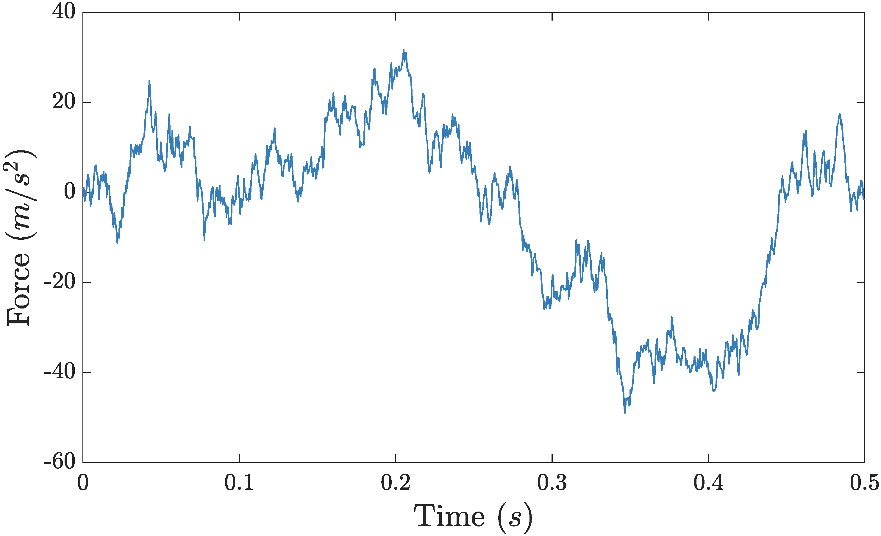
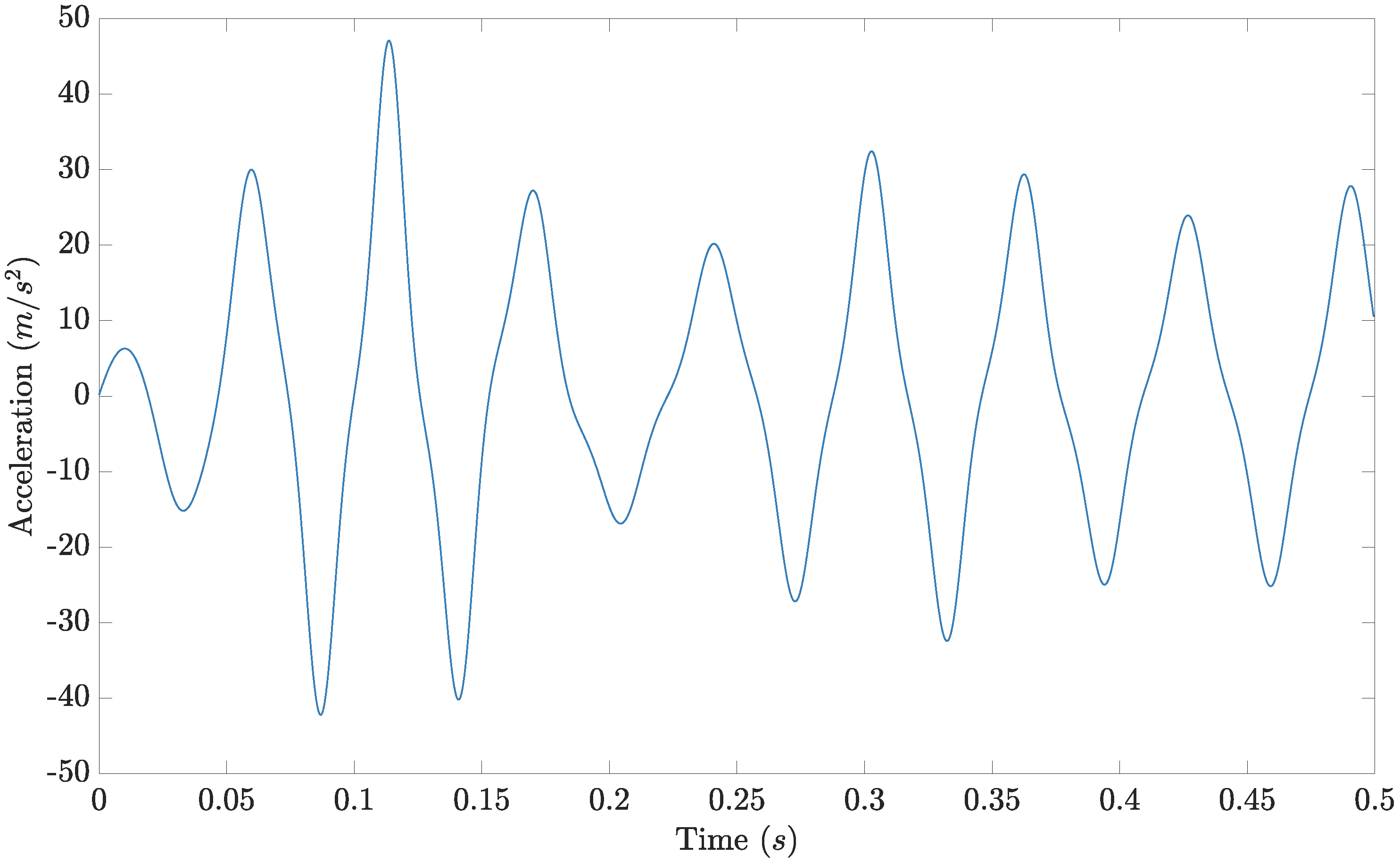
The acceleration of the oscillator with this added measurement noise is shown in Figure 2 and the time history of the force which generated this response is seen in Figure 3. The frequency content of the forcing applied is sufficiently rich to ensure that the system responds with rich dynamic behaviour.
The methodolgy described in Section 2 can be readily applied with little user modification. The Duffing oscillator is first rewritten as a nonlinear state-space model with two states the displacement and the velocity,
z ˙ z ¨ = z ˙ U m k m z c m z ˙ k 3 m z 3 = z ˙ U m 1 m h ( z , z ˙ )
This model is then combined with the state space form of the chosen kernel, in this case a Matérn 1/2 kernel is used to give the continuous time model,
z ˙ z ¨ u ˙ = z ˙ u m 1 m h ( z , z ˙ ) λ u + 0 0 1 w ( t )
where λ and w ( t ) are related to the hyperparameters of the GP kernel as described.
Algorithm 5 is run to perform the joint input-state estimation on the system and recover samples from the full joint posterior over the states and the hyperparameters p ( x 1 : T , θ | y 1 : T ) . The algorithm is run for 1 × 10 5 iterations (i.e., J = 100 , 000 ) and the first 10,000 samples are discarded as burn-in (Code used in this experiment can be found at https://github.com/TimothyRogers/vibration-NL-input-state). The states are sampled every five iterations, which helps with stability in sampling the parameters. The proposal for the particle filter in Algorithm 4 is a bootstrap filter with the number of particles set to fifty. With these algorithm settings the computation takes close to two hours to complete (with some variation between runs) on a commercially availabile laptop computer (CPU:Intel i7-8550U 1.80 GHz, 16 GB RAM). It is worth noting that the code has been written by the authors in Matlab and not fully optimised for speed, for example the possible parallelisation of the algorithm has not been fully exploited and it is expected that the computational time and “wall-clock time” could be significantly reduced with further consideration of the software.
Algorithm 5 A Blocked Gibbs Sampler for Joint Input-State Estimation
  1:
Set x 1 : T ( 0 ) and θ ( 0 )
  2:
for j = 1 , , J do
  3:
      Set x 1 : T x 1 : T ( j 1 )
  4:
      Sample x 1 : T | θ ( j 1 ) according to Algorithm 4
  5:
      Set x 1 : T ( j ) x 1 : T
  6:
      Sample θ ( j ) | x 1 : T ( j ) K θ ( j 1 ) , x 1 : T ( j ) , ·
  7:
end for
To form the transition density of the state-space model it is necessary to discretise the nonlinear stochastic differential equation, an Euler-Maruyama method [32] is used to do this. This discretisation was found to be an acceptable approach for the results shown here, however, it is relatively simple to use a higher-order discretisation if desired [33]. For this case study, uninformative priors are used for the hyperparameters in a transformed space which ensures they remain positive. It is strongly advsied, however, that should prior information be available, it is incorporated. Including proper priors for the hyperparameters will aid identifiability and improve the efficiency of the inference.
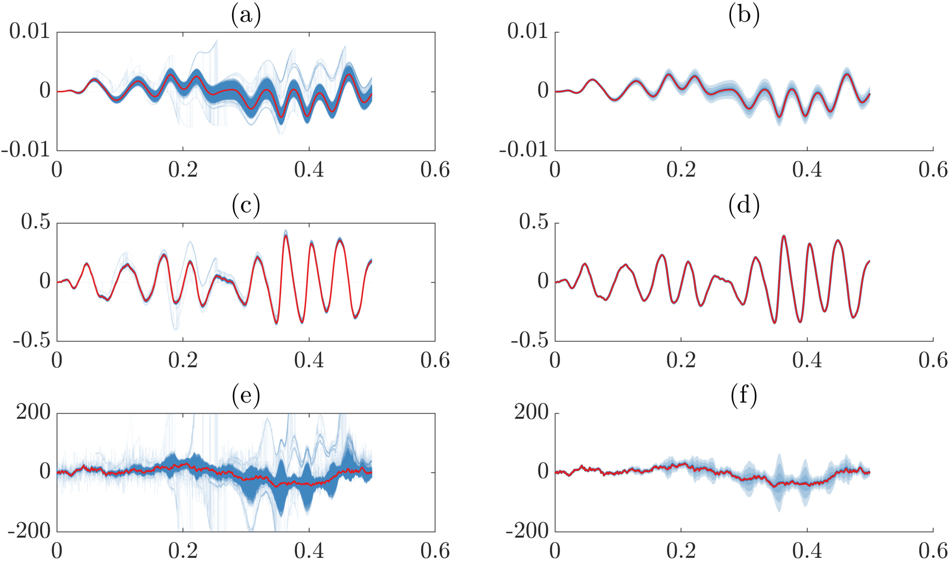
The resulting samples from the MCMC inference over the smoothing distributions of the states are shown in Figure 4. The full set of samples is shown in the left three frames (a), (c) and (e) which correspond to the displacement, velocity and unknown input force respectively (Note: the y-axis limits have been truncated in Figure 4 frame (e) to increase legibility; the full limits are shown in Figure 5.). On the right hand side of Figure 4 the distributions over the states at each time step have been approximated by computing the first two moments of the empirical distribution at each point in time. The uncertainty in the distributions is shown by shading in progressively lighter colours from one to three standard deviations from the mean. For each state, the ground truth values for the state trajectories are shown in red.
From these plots it is clear to see that the states have been well approximated by the MCMC inference. The ground truth passes through all the sample distributions and in the approximate distributions shown in frames (b), (d), (f) of the ground truth is very close to the mean. To measure this a Normalised Mean-Squared Error metric is computed using the following formula,
N M S E = 100 T σ x 2 t = 1 T x t x ˆ t 2
where x is the true value, x ˆ the estimated value (in this case the mean of the samples of the states at time t), T the number of time points and σ x 2 the variance of the ground truth as the model. This metric has some desirable properties in its interpretability, a score of zero indicates a perfect match with the ground truth, a score of 100 is equivalent to simply taking the mean of the ground truth. The NMSE scores for the three states; displacement, velocity and estimated force are 0.10 %, 5.4 × 10 4 % and 0.31% respectively. These values indicate that the expected values of the states very closely align with the ground truth and that they provide accurate estimates of those quantities.
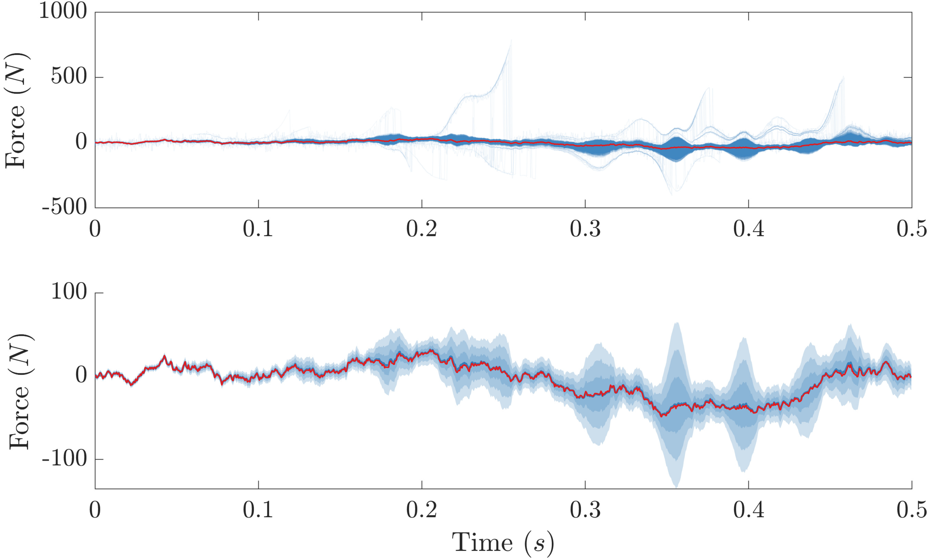
The uncertainty present in the estimates is also of interest, since this was argued as a strength of the Bayesian approach. The quality of the uncertainty estimation is somewhat harder to quantify; however, it can be seen from Figure 4 that the uncertainty is, visually, captured well. Considering the velocity state, which has very low uncertainty throughout the time history, it is reassuring that the mean response in this state is also the closest match to the ground truth—by some margin. This pattern continues where the greatest uncertainty is seen in the forcing state which is also the state with the highest NMSE score—although this score is still very low. Considering more closely this forcing state, which is shown again in Figure 5, it can be see that this is the state which has been hardest to identify. Increased uncertainty is seen, especially around 0.3 s , 0.35 s and 0.4 s . Also considering the samples from this state it can be seen that there have been several samples which deviate significantly from the bulk of the probability mass. Since the observation density mean quantity is dominated by the dynamic response of the oscillator not the shoot-through of the force, perhaps this is to be expected, although it does warrant futher investigation in a later work. One other interesting feature of the recovered distributions is the reduction in variance close to the beginning of the time history. This could be due to poor mixing in the MCMC; however, investigating this it is found that the chain is well mixed. It is suspected that this behaviour is due to the initial conditions of the state-space model having a small prior variance; this again may be an avenue for future investigation.
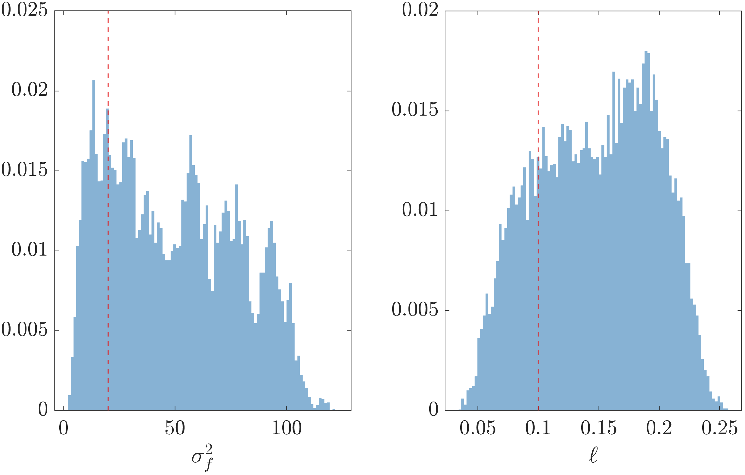
Although the primary object of interest in this work is the smoothing distribution over the states— which recovers the internal states of the oscillator and the unknown inputs—it is also worthwhile investigating the posterior distributions of the hyperparameters. Figure 6 shows the histograms of the marginal posterior densities for each of the hyperparameters with the ground truth value shown by a dashed red line. It can be seen that the posterior distributions for these parameters appear to be more complicated than might be expected. It is reassuring that the ground truth values lie within the bulk of the probability mass of the distributions, but it may be concerning that the maximum a posteriori value for the length scale does not coincide with the ground truth. This behaviour of the distribution is, in fact, expected when identifying hyperparameters of a Gaussian process. It is known that there is significant correlation between the signal variance σ f 2 and the lengthscale and that this can lead (when optimising these quantities) to two different but similarly “good” solutions. This phenomenon has been studied in the context of emulating computer models [34], but is equally relevant here.
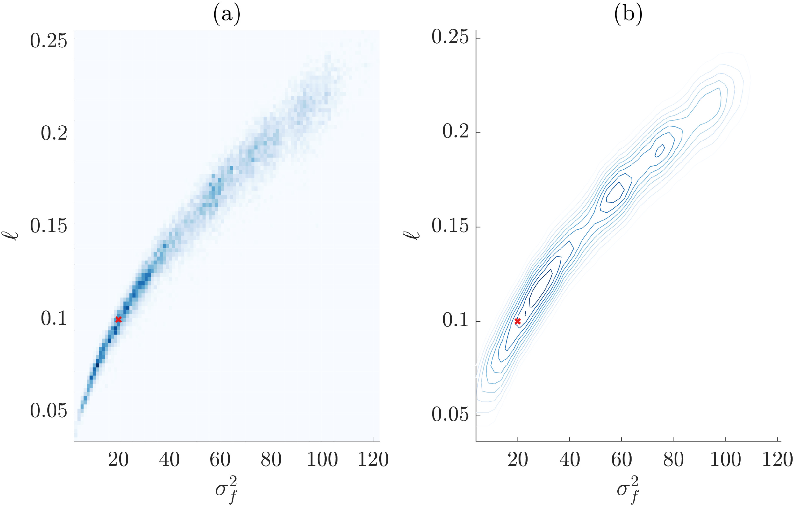
This interplay between the hyperparameters gives rise to a characteristic “elbow-shaped” posterior distribution, this is also discussed in [25]. When considering the joint posterior of the hyperparameters this correlation can be clearly seen. In Figure 7, the density of samples in the posterior is shown as a two-dimensional histogram in frame (a) where the darker blue indicates a higher density and in frame (b) as a contour plot. It can be seen that the Gibbs sampler is exploring the posterior which trades off the length scale and the signal variance of the Gaussian process to find a plausible set of hyperparameters. In the two dimensional figure it is more apparent that the ground truth values for the hyperparameters lie very comfortably in the bulk of the probability mass of the distribution. The increased uncertainty around these hyperparameters is not a concern, as it reveals the inherent distribution of solutions available when choosing a GP as the model for the unknown force.
This section has served as a case study on the application of the methodology presented. It has been seen that by applying this approach to joint input-state estimation it is possible to recover distributions over the unknown states in the model, which have now been augmented with the unmeasured force. It was also seen that the distribution over the hyperparameters of the GP which is chosen to model this unknown force can be simultaneously inferred alongside the states leading to a fully Bayesian solution.
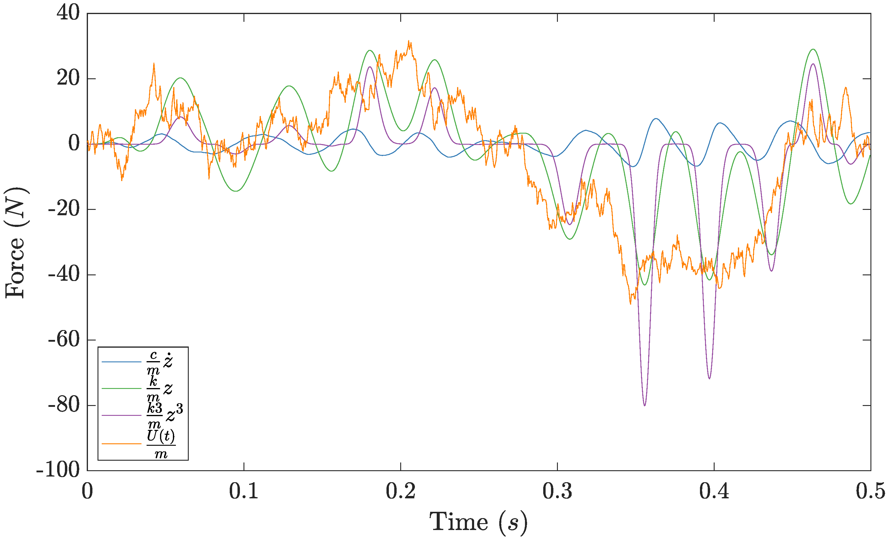
Investigating this uncertainty it appears that, there is the greatest uncertainty in the estimate of the external force state when the nonlinear term is contributing more to the restoring force in the oscillator; this is visible in Figure 8, where each of the terms of the equation of motion are shown individually. This relationship is an interesting behaviour of the technique and one which may be a valuable avenue of futher investigation.

4. Conclusions

This paper has presented a methodology for joint input-state estimation for nonlinear systems based on a particle Gibbs identification of a nonlinear Gaussian process latent force model. It has been shown how, for a given nonlinear system, the forcing on that system can be assumed to be some Gaussian process in time whose behaviour is governed by a covariance kernel. With the correct choice of this kernel the GP can be converted into a linear Gaussian state-space model. This is then used to augment a state space representation of the nonlinear system.
In possession of this nonlinear state-space model, which represents the dynamics of the system and the unknown force, the task is to infer the smoothing distributions of that model and the distributions of the unknown hyperparameters. It was shown here how a particle Gibbs approach could be used to solve this problem. The Particle Gibbs with Ancestor Sampling kernel is used to efficiently draw samples from the smoothing distribution of the states. A Metropolis-Hastings kernel is then used to draw samples for the hyperparameters conditioned on the sampled states.
The effectiveness of this methodology was shown in a numerical case study of a Duffing oscillator. It was seen that the approach is able to recover the input to the system and the internal states of the oscillator. The MCMC procedure produced a set of samples from the smoothing distribution which captured well the uncertainty in the model; this was futher evidenced by considering a Gaussian approximation based on the first two moments of the samples at each time step. The mean of the sampled distribution showed very low NMSE scores, indicating that the maximum a posteriori estimates of the inferred distribution are accurate with respect to the ground truth. The results also show increased uncertainty in the forcing state relative to the displacement or velocity.

Future Work

While the method shown here represents a reasoned and powerful approach to the nonlinear input-state estimation problem, there is further investigation to be carried out. It will be of interest to investigate the performance of the model in hysteretic systems, a task which should be possible within this model form but which has not been explicitly shown here. The performance of the method with increasing “strength” of nonlinearity also bears investigation. If the trend of increasing uncertainty with increased contribution of the nonlinear terms in the model continues, whether the methodology breaks down at high forcing levels should be investigated. Likewise, the performance of this approach when the oscillator is pushed into a chaotic regime also requires further investigation; in that situation it is likely that this method would struggle to separate the forcing from the dynamics of the system. Finally, two obvious extensions to the method which should be shown are the extension to joint input-state estimation in the MDOF case and the extension of this approach to include parameter estimation in the nonlinear system. It is expected that extending this methodology to the joint input-state-parameter case will significantly increase the difficulty in inference. This difficultly will arise from a non-identifiability between the nonlinear components and the external force components in the equation of motion. As the complexity of the system increases in terms of the number of degrees of freedom, to a very high number then there will be two major barriers to application of the proposed methodolgy. The first will be purely computational, increasing the number of states in the model will require a larger number of particles to be included in the filter and it will become infeasible to accurately compute the filtering or smoothing distributions. Likewise, if the complexity of the system increases due to emergent dynamics or chaotic behaviour then the authors would not recommended application of this methodolgy. This does warrant further investigation, but the number of required particles to recover the hidden states would need to be significantly increased again leading to computational infeasibility.
In conclusion, this paper has shown a methodolgy for performing joint input-state estimation on nonlinear systems in a Bayesian manner with a focus on uncertainty quantification in the estimation. It has been shown that the nonlinear Gaussian process latent force approach can accurately recover an unknown input to a nonlinear sytem using a particle Gibbs inference procedure. This work opens up the possibility of input-state estimation on more complicated nonlinear systems and even joint input-state-parameter schemes.

Author Contributions

Conceptualization, T.J.R.; methodology, T.J.R.; software, T.J.R.; validation, T.J.R.; investigation, T.J.R.; writing—original draft preparation, T.J.R.; writing—review and editing, T.J.R., K.W. and E.J.C. All authors have read and agreed to the published version of the manuscript.

Funding

This research was funded by the Engineering and Physical Sciences Research Council (EPSRC), UK grant number EP/S001565/1 and EP/R003645/1. The APC was funded by University of Sheffield.

Acknowledgments

The authors would also like to thank Fredrik Lindsten for some very helpful discussions on particle MCMC.

Conflicts of Interest

The authors declare no conflict of interest.

Appendix A. Sine Wave Input Example

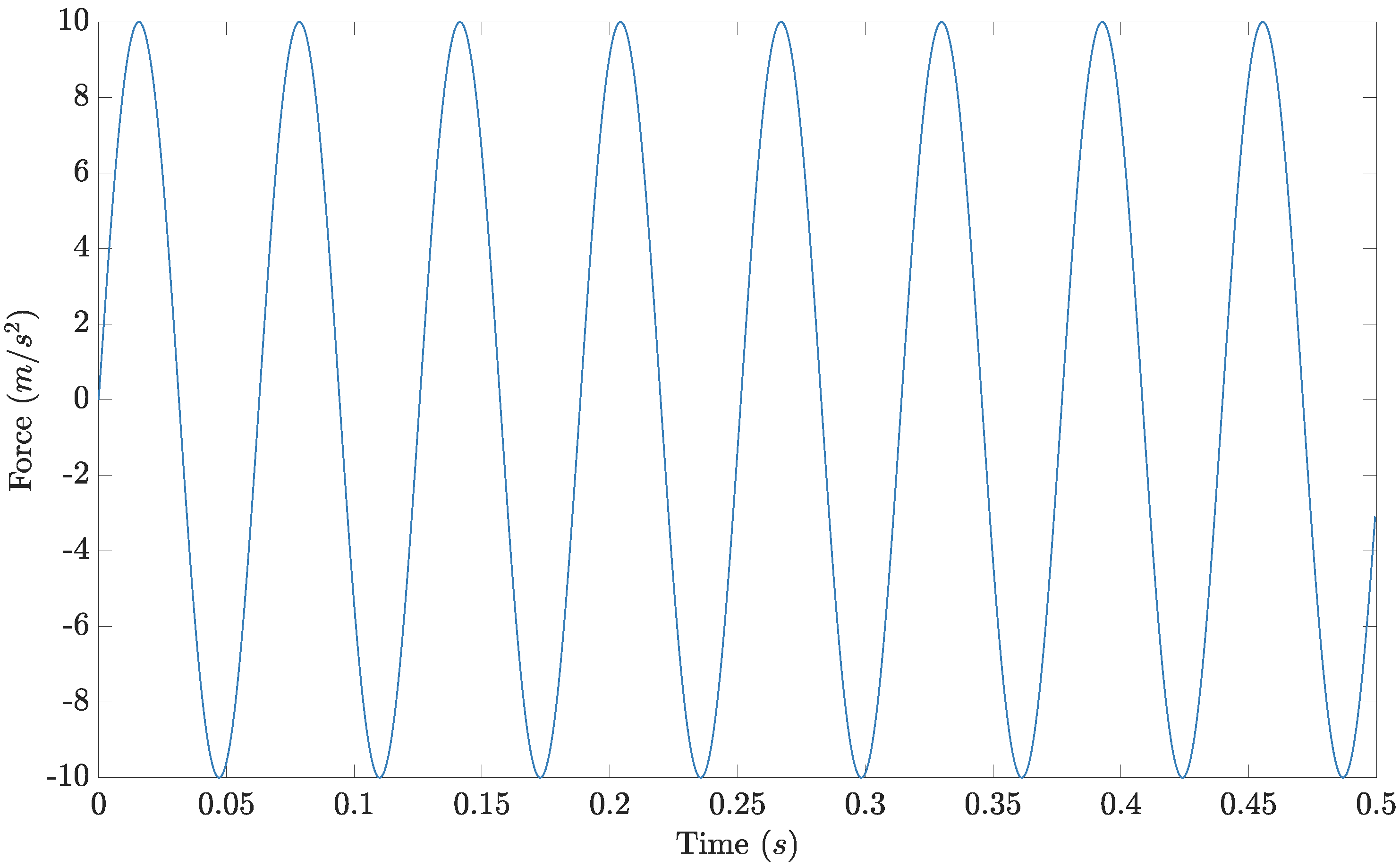
In this appendix, a second application of the method is shown. The setup is unchanged from that used in Section 3, except that the forcing on the system is now chosen to be a sine wave with an amplitude of 10 and a frequency of 100 rad (equal to the natural frequency of the linear system k / m ).
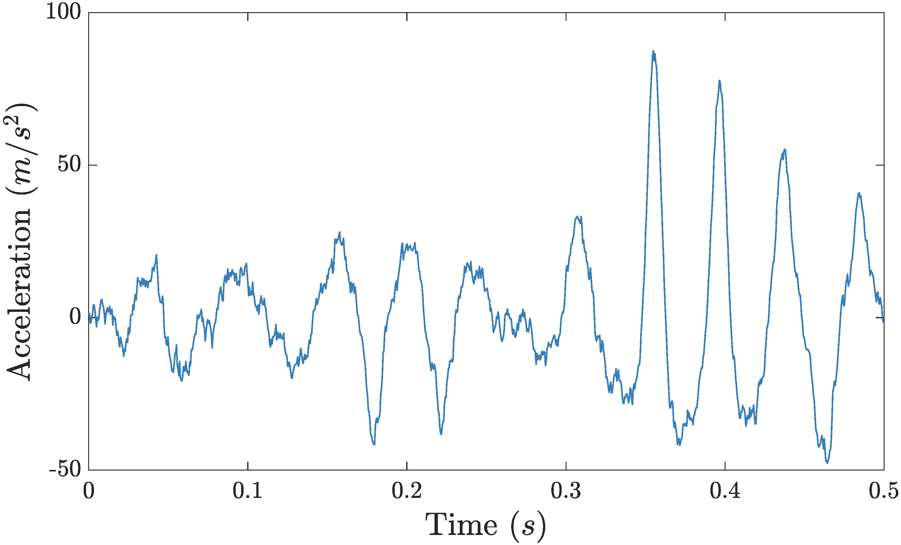
The acceleration of the oscillator with the same added measurement noise of 1% RMS is shown in Figure A1 and the time history of the the sine wave which is the specified external forcing is seen in Figure A2.
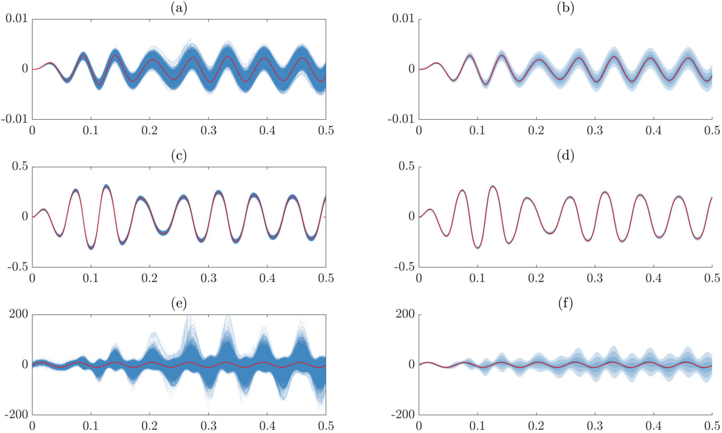
Performing this inference as before leads to the results seen in Figure A3 for recovery of the state smoothing distributions. The observed results are very similar in quality to the case study shown in Section 3. The displacement and velocity states show lower but plausible uncertainty in the samples, which is well approximated by a Gaussian distribution at each time step. The uncertainty in the forcing state is higher, as may be expected due to the mismatch between the prior Gaussian process and the sine wave input; however, the uncertainty reflects the difficulty in precisely recovering this unmeasured quantity.
Figure A1. Measured acceleration from the Duffing oscillator.
Vibration 03 00020 g0a1
Figure A2. Ground truth forcing time history applied to the oscillator.
Vibration 03 00020 g0a2
Specifying the same Matérn 1/2 kernel and dynamic model as before, the same MCMC inference scheme is run, 1 × 10 5 samples are taken with a burn-in of 10,000 samples where the states are sampled every 5 iterations. An identical model for the dynamics in the state-space model is used.
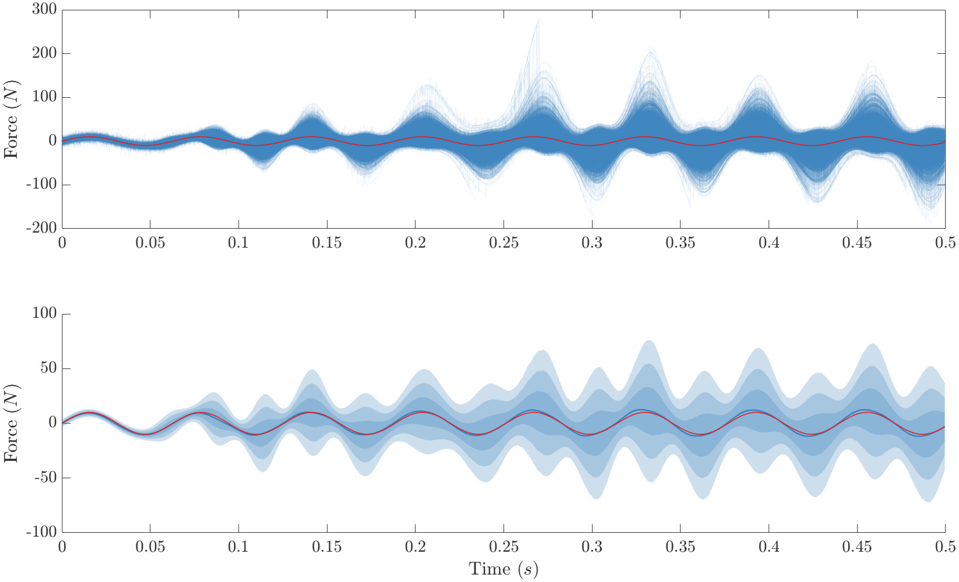
Inspecting more closely the estimate of the sine wave forcing (Figure A4) it can be seen that the mean of the samples aligns well with the known deterministic forcing giving a normalised mean-squared error of 3.2%. This set of results for the sine wave input is expected but still reassuring. The flexibility of the GP prior over the forcing function allows the posterior of the smoothing distribution to move to the true forcing that the system has experienced with very little prior modelling input from the user, provided a model of the system itself is available. As has been mentioned in the main text, this should mean that a diverse set of inputs can be recovered, provided they can be represented under the prior.
Figure A3. Paths sampled using the PGAS kernel for the three states in the model, on the left in (a,c,e) the samples in blue from the MCMC; on the right in (b,d,f) a Gaussian approimation of the posterior at every time step showing the mean in solid blue and one, two and three standard deviations shaded in blue. The ground truth values for the displacement, velocity and force are superimposed in red.
Vibration 03 00020 g0a3
Figure A4. In the upper frame, samples from the MCMC inference of the states for the state corresponding to the unknown forcing on the Duffing oscillator. The samples are shown in blue with the ground truth superimposed in red. In the lower frame, the result of taking a Gaussian approximation at every time step. The mean of the samples is shown as a solid blue line, the intervals at one, two and three standard deviations are shaded in blue. The ground truth is, again, superimposed in red.
Vibration 03 00020 g0a4

References

  1. Andrieu, C.; Doucet, A.; Holenstein, R. Particle Markov chain monte carlo methods. J. R. Stat. Soc. Ser. B (Stat. Methodol.) 2010, 72, 269–342. [Google Scholar] [CrossRef] [Green Version]
  2. Naets, F.; Cuadrado, J.; Desmet, W. Stable force identification in structural dynamics using Kalman filtering and dummy-measurements. Mech. Syst. Signal Process. 2015, 50, 235–248. [Google Scholar] [CrossRef]
  3. Azam, S.E.; Chatzi, E.; Papadimitriou, C. A dual Kalman filter approach for state estimation via output-only acceleration measurements. Mech. Syst. Signal Process. 2015, 60, 866–886. [Google Scholar] [CrossRef]
  4. Maes, K.; Karlsson, F.; Lombaert, G. Tracking of inputs, states and parameters of linear structural dynamic systems. Mech. Syst. Signal Process. 2019, 130, 755–775. [Google Scholar] [CrossRef]
  5. Nayek, R.; Chakraborty, S.; Narasimhan, S. A Gaussian process latent force model for joint input-state estimation in linear structural systems. Mech. Syst. Signal Process. 2019, 128, 497–530. [Google Scholar] [CrossRef] [Green Version]
  6. Rogers, T.; Worden, K.; Manson, G.; Tygesen, U.; Cross, E. A Bayesian filtering approach to operational modal analysis with recovery of forcing signals. In Proceedings of the ISMA 2018-International Conference on Noise and Vibration Engineering and USD 2018-International Conference on Uncertainty in Structural Dynamics, Leuven, Belgium, 17–19 September 2018. [Google Scholar]
  7. Naets, F.; Croes, J.; Desmet, W. An online coupled state/input/parameter estimation approach for structural dynamics. Comput. Methods Appl. Mech. Eng. 2015, 283, 1167–1188. [Google Scholar] [CrossRef]
  8. Dertimanis, V.K.; Chatzi, E.; Azam, S.E.; Papadimitriou, C. Input-state-parameter estimation of structural systems from limited output information. Mech. Syst. Signal Process. 2019, 126, 711–746. [Google Scholar] [CrossRef]
  9. Ding, Y.; Zhao, B.; Wu, B.; Zhang, X.; Guo, L. Simultaneous identification of structural parameter and external excitation with an improved unscented Kalman filter. Adv. Struct. Eng. 2015, 18, 1981–1998. [Google Scholar] [CrossRef]
  10. Rogers, T.; Worden, K.; Cross, E. On the application of Gaussian process latent force models for joint input-state-parameter estimation: With a view to Bayesian operational identification. Mech. Syst. Signal Process. 2020, 140, 106580. [Google Scholar] [CrossRef]
  11. Lei, Y.; Xia, D.; Erazo, K.; Nagarajaiah, S. A novel unscented Kalman filter for recursive state-input-system identification of nonlinear systems. Mech. Syst. Signal Process. 2019, 127, 120–135. [Google Scholar] [CrossRef]
  12. Erazo, K.; Nagarajaiah, S. An offline approach for output-only Bayesian identification of stochastic nonlinear systems using unscented Kalman filtering. J. Sound Vib. 2017, 397, 222–240. [Google Scholar] [CrossRef]
  13. Yuen, K.V.; Beck, J.L. Updating properties of nonlinear dynamical systems with uncertain input. J. Eng. Mech. 2003, 129, 9–20. [Google Scholar] [CrossRef] [Green Version]
  14. Kalman, R.E. A new approach to linear filtering and prediction problems. J. Basic Eng. 1960, 82, 35–45. [Google Scholar] [CrossRef] [Green Version]
  15. Rauch, H.E.; Striebel, C.; Tung, F. Maximum likelihood estimates of linear dynamic systems. AIAA J. 1965, 3, 1445–1450. [Google Scholar] [CrossRef]
  16. Julier, S.J.; Uhlmann, J.K.; Durrant-Whyte, H.F. A new approach for filtering nonlinear systems. In Proceedings of the 1995 IEEE American Control Conference, Seattle, WA, USA, 21–23 June 1995; Volume 3, pp. 1628–1632. [Google Scholar]
  17. Julier, S.J.; Uhlmann, J.K. New extension of the Kalman filter to nonlinear systems. In Signal Processing, Sensor Fusion, and Target Recognition VI; International Society for Optics and Photonics: Bellingham, WA, USA, 1997; Volume 3068, pp. 182–194. [Google Scholar]
  18. Wan, E.A.; Van Der Merwe, R. The unscented Kalman filter for nonlinear estimation. In Proceedings of the IEEE 2000 Adaptive Systems for Signal Processing, Communications, and Control Symposium (Cat. No.00EX373), Lake Louise, AB, Canada, 4 October 2000; pp. 153–158. [Google Scholar]
  19. Särkkä, S. Bayesian Filtering and Smoothing; Cambridge University Press: Cambridge, UK, 2013. [Google Scholar]
  20. Doucet, A.; Johansen, A.M. A tutorial on particle filtering and smoothing: Fifteen years later. Handb. Nonlinear Filter. 2009, 12, 3. [Google Scholar]
  21. Pitt, M.K.; Shephard, N. Auxiliary variable based particle filters. In Sequential Monte Carlo Methods in Practice; Springer: New York, NY, USA, 2001; pp. 273–293. [Google Scholar]
  22. Rogers, T.; Schön, T.; Lindholm, A.; Worden, K.; Cross, E. Identification of a Duffing oscillator using particle Gibbs with ancestor sampling. J. Phys. Conf. Ser. 2019, 1264, 012051. [Google Scholar] [CrossRef]
  23. Alvarez, M.; Luengo, D.; Lawrence, N. Latent force models. In Proceedings of the Artificial Intelligence and Statistics, Clearwater Beach, FL, USA, 16–18 April 2009; pp. 9–16. [Google Scholar]
  24. O’Hagan, A.; Kingman, J. Curve fitting and optimal design for prediction. J. R. Stat. Soc. Ser. (Methodol.) 1978, 40, 1–42. [Google Scholar] [CrossRef]
  25. Rasmussen, C.E.; Williams, C.K.I. Gaussian Processes for Machine Learning; The MIT Press: Cambridge, MA, USA, 2005. [Google Scholar]
  26. Hartikainen, J.; Särkkä, S. Kalman filtering and smoothing solutions to temporal Gaussian process regression models. In Proceedings of the 2010 IEEE International Workshop on Machine Learning for Signal Processing (MLSP), Kittila, Finland, 29 August–1 September 2010; pp. 379–384. [Google Scholar]
  27. Hartikainen, J.; Sarkka, S. Sequential inference for latent force models. arXi 2012, arXiv:1202.3730. [Google Scholar]
  28. Stein, M.L. Interpolation of Spatial Data: Some Theory for Kriging; Springer: Berlin/Heidelberg, Germany, 1999. [Google Scholar]
  29. Lindsten, F.; Jordan, M.I.; Schön, T.B. Particle Gibbs with ancestor sampling. J. Mach. Learn. Res. 2014, 15, 2145–2184. [Google Scholar]
  30. Gelman, A.; Carlin, J.B.; Stern, H.S.; Dunson, D.B.; Vehtari, A.; Rubin, D.B. Bayesian Data Analysis; CRC Press: Boca Raton, FL, USA, 2013. [Google Scholar]
  31. Kovacic, I.; Brennan, M.J. The Duffing Equation: Nonlinear Oscillators and Their Behaviour; John Wiley & Sons: Hoboken, NJ, USA, 2011. [Google Scholar]
  32. Särkkä, S.; Solin, A. Applied Stochastic Differential Equations; Cambridge University Press: Cambridge, UK, 2019; Volume 10. [Google Scholar]
  33. Kloeden, P.E.; Platen, E. Numerical Solution of Stochastic Differential Equations; Springer Science & Business Media: Berlin/Heidelberg, Germany, 2013; Volume 23. [Google Scholar]
  34. Andrianakis, I.; Challenor, P.G. The effect of the nugget on Gaussian process emulators of computer models. Comput. Stat. Data Anal. 2012, 56, 4215–4228. [Google Scholar] [CrossRef]
Figure 1. The graphical model of a general probabilistic state-space model.
Vibration 03 00020 g001
Figure 2. Measured acceleration from the Duffing oscillator.
Vibration 03 00020 g002
Figure 3. Ground truth forcing time history applied to the oscillator.
Vibration 03 00020 g003
Figure 4. Paths sampled using the PGAS kernel for the three states in the model, on the left in (a,c,e) the samples in blue from the MCMC; on the right in (b,d,f) a Gaussian approimation of the posterior at every time step showing the mean in solid blue and one, two and three standard deviations shaded in blue. The ground truth values for the displacement, velocity and force are superimposed in red.
Vibration 03 00020 g004
Figure 5. In the upper frame, samples from the MCMC inference of the states for the state corresponding to the unknown forcing on the Duffing oscillator. The samples are shown in blue with the ground truth superimposed in red. In the lower frame, the result of taking a Gaussian approximation at every time step. The mean of the samples is shown as a solid blue line, the intervals at one, two and three standard deviations are shaded in blue. The ground truth is, again, superimposed in red.
Vibration 03 00020 g005
Figure 6. Histograms of the marginal distributions for each hyperparameter from the MCMC samples, the ground truth is indicated with the red dashed line.
Vibration 03 00020 g006
Figure 7. In frame (a), the joint posterior of the hyperparameters as a two-dimensional histogram, with darker areas indicating higher density. In frame (b), a contour plot from estimating this joint density using convolution over the two-dimensional histogram. On both plots the ground truth is indicated with the red cross (x).
Vibration 03 00020 g007
Figure 8. The individual ground truth terms contributing to the motion of the oscillator.
Vibration 03 00020 g008