1. Introduction
Wildfire smoke exposure has increased sharply across the United States in recent decades, and smoke now contributes a growing fraction of fine particulate matter (PM
2.5) pollution [
1,
2]. Consistent with this trend, burned area in the western United States has increased approximately fourfold since the 1980s [
3,
4]. In some western regions, wildfire smoke has accounted for up to half of ambient PM
2.5 in recent years [
5,
6]. These smoke episodes produce short-lived but intense PM
2.5 spikes locally, while longer-range transported smoke contributes additional episodic pollution over broader regions [
7,
8,
9]. A growing body of epidemiologic evidence links wildfire-attributable PM
2.5 to increased all-cause, cardiovascular, respiratory mortality, and other cardiopulmonary conditions [
10,
11,
12,
13,
14,
15,
16], as well as adverse birth outcomes and mental-health effects [
17,
18]. Collectively, these findings underscore the urgent need to better understand and mitigate pollution exposure to wildfire smoke.
To date, most studies estimate wildfire smoke exposure using outdoor ambient PM
2.5 measurements. However, outdoor concentrations do not fully capture personal exposure because people in the United States spend about 93% of their time in enclosed buildings and vehicles [
19]. While public health agencies recommend remaining indoors during smoke events to reduce exposure, indoor environments are not fully insulated from outdoor smoke [
20]. Wildfire-related PM
2.5 can infiltrate buildings through leaks, open windows and doors, and mechanical ventilation systems [
21,
22]. The extent of infiltration varies widely across buildings, ventilation systems, and occupant behaviors [
23]. Hence, indoor PM
2.5 concentrations can rise substantially during smoke episodes and may approach outdoor concentrations [
24,
25,
26].
Under routine (non-fire) conditions, the determinants of indoor–outdoor PM
2.5 exchange are reasonably well understood at the building level but are difficult to characterize across large, heterogeneous housing stocks [
21,
27]. Outdoor particles enter indoor areas through leakage and ventilation, while filtration and deposition affect how long they remain suspended [
22,
27,
28]. These processes are often summarized by the “infiltration factor” [
29], which reflects particle penetration, air exchange rate, and indoor loss. In practice, infiltration factors vary widely across homes due to differences in construction, HVAC configuration, operation and filter efficiency, indoor sources, and resuspension [
29,
30,
31,
32].
Wildfire smoke presents a different exposure context. Outdoor concentrations can be extremely high and fluctuate quickly over hours to days; smoke particles can differ from typical urban PM [
33,
34]. Smoke episodes also trigger heterogeneous behavioral and operational responses that can either reduce or amplify indoor exposure. Additionally, occupants may remain indoors longer, close windows and exterior doors, switch HVAC systems to recirculation, upgrade filters, or run portable cleaners [
35,
36,
37,
38], whereas heat stress or power outages may increase window opening or limit filtration [
39], increasing infiltration. Hence, the indoor PM
2.5 burden during smoke events is jointly determined by fast-changing outdoor concentrations and concurrent changes in building operation and human behavior.
Recent fire-season studies [
24,
25,
26], including targeted field monitoring and analyses of crowdsourced sensors, have begun to quantify how wildfire smoke affects indoor air. One large California study using more than 2.4 million sensor-hours from over 1400 buildings in the PurpleAir network [
24] found that mean infiltration ratios (indoor PM
2.5 of outdoor origin divided by outdoor PM
2.5) dropped from about 0.4 on non-fire days to 0.2 on wildfire days, yet indoor PM
2.5 still nearly tripled during smoke episodes. A year-long [
40] campaign at four skilled nursing facilities in the western United States reported 24 h indoor PM
2.5 peaks up to 200 µg/m
3 and infiltration efficiencies ranging from 0.22 to 0.76 across facilities, highlighting the importance of building characteristics and operation. Intervention studies [
31] further show that filtration and behavior can substantially reduce indoor smoke concentrations. Together, these studies suggest that although mitigation can reduce infiltration on smoke days, indoor exposure remains highly context-dependent.
Despite this progress, key gaps remain. Much of the literature focuses on single regions (primarily the western United States), specific building types, and one or a few fire seasons, which constrains generalizability across climates, housing stocks, and policy contexts [
24,
25,
26,
41]. In addition, outcomes are often summarized as indoor-to-outdoor ratios or infiltration factors that assume near-steady conditions [
21,
42,
43], which may be less informative when outdoor concentrations change rapidly during smoke plumes. Many analyses [
25,
26] also rely on cross-sectional summaries rather than longitudinal time-series frameworks that adjust for confounders to quantify how wildfire smoke alters the outdoor–indoor PM
2.5 difference. These limitations highlight the need for large-scale longitudinal analyses across diverse geographic settings that both use meteorology-adjusted time-series models to quantify smoke-associated shifts in the outdoor–indoor PM
2.5 difference and characterize heterogeneity in indoor protection through data-driven response patterns rather than a single summary ratio during wildfire events.
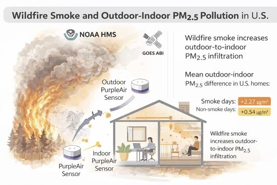
We address this need by leveraging a large U.S. dataset of paired indoor and nearby outdoor PM2.5 measurements from 2019 to 2024 across diverse climate zones. We first use meteorology-adjusted time-series models to estimate how smoke days differ from non-smoke days in the outdoor–indoor PM2.5 difference, adjusting for temperature, humidity, and temporal variation. We then use an unsupervised clustering approach as a complementary descriptive tool to summarize recurring outdoor–indoor response modes on smoke days, identifying distinct and interpretable patterns in which smoke-day changes are dominated by increases in outdoor concentration, smaller indoor responses relative to outdoor changes, or by both. We address three related questions: whether the outdoor–indoor PM2.5 difference is larger on smoke days than on non-smoke days; whether increases in this difference are driven primarily by larger outdoor PM2.5 increases, smaller indoor PM2.5 responses, or both; and whether these smoke-day response patterns vary geographically across broad U.S. climate regions represented in the monitored samples. Together, these analyses provide a quantitative assessment of indoor PM2.5 during wildfire events, clarify when and where indoor environments offer meaningful protection, and inform exposure mitigation and public-health guidance.
2. Methods
2.1. Sensor Data Acquisition, Quality Control, and Calibration
PurpleAir is a citizen science–based, low-cost air quality monitoring network that provides high-resolution, real-time particulate matter (PM) measurements. Each PurpleAir PA-II monitor (PurpleAir, Inc., Draper, UT, USA) contains two Plantower PMS5003 optical particle counters (Plantower, Beijing, China), corresponding to channels A and B, that measure the same underlying particle signal and provide two parallel PM2.5 estimates for quality assurance. The monitor reports minute-level PM2.5 using two processing outputs: (1) the Plantower factory algorithm (“ATM”) and (2) a U.S. EPA correction (“CF1”), which applies a different formula to derive PM2.5 and is generally more appropriate for indoor environments. In addition, the sensors report temperature and relative humidity (RH).
PurpleAir metadata do not provide a standardized verified building-use classification for all indoor sensors. To better characterize the indoor environments represented in the analytic sample, we reviewed the sensor name metadata for the indoor monitors retained after all quality-control and pairing procedures. This review suggested that the indoor sensors represented a heterogeneous mix of indoor environments, including some residential/private settings and some clearly non-residential settings, although many sensor names were generic or too unclear to classify confidently.
We retrieved minute-level data from 13,487 PurpleAir sensors located in the contiguous United States (2019–2024) via the U.S. EPA RSIG3D PurpleAir data inventory. We applied a standardized preprocessing and quality-control workflow to generate analysis-ready PM2.5 time series. First, the channel A and B measurements were temporally aligned. We excluded sensor-days with poor inter-channel agreement (Pearson R2 < 0.75 based on ATM values). The remaining minute-level observations were aggregated to hourly means; sensor-days with fewer than 18 valid hourly observations were removed. Daily averages were then computed from qualified hourly data. The sensors were classified as indoor or outdoor using PurpleAir metadata.
To ensure internal consistency, observations were retained only when the absolute difference between channels was <5 µg/m3 and the relative difference (absolute difference divided by the channel mean) was <2. To identify anomalous meteorological values, RH, temperature, and pressure outliers were removed using a robust median absolute deviation (MAD; Hampel) filter. For each residence and variable, rolling 7-day medians and scaled MADs (×1.4826) were computed, and observations exceeding 6 MAD from the local median were flagged as missing. When data density was insufficient, the rolling window was expanded to 14 days or to the full available time series.
All primary analyses were conducted using the Plantower CF1 PM
2.5 measurements. Measurement consistency was assessed using Pearson correlations, computed within each paired indoor–outdoor monitor set and indexed by the indoor monitor identifier (indoor ID), which served as the pair ID throughout.
Supplementary Figure S1 shows within-sensor agreement between CF1 channels for randomly selected monitors. Pearson correlations ranged from ~0.87 to 1.00 (median ≈ 0.99). Points lay close to the 1:1 line in all panels, and all retained monitors exceeded the screening threshold (R
2 ≥ 0.75), supporting use of the channel average in subsequent analyses. Corrected PM
2.5 concentrations were obtained using the U.S.-specific PurpleAir correction developed and validated by Barkjohn et al. (2021) [
44], applied to the CF1 values after averaging channels A and B and implemented separately for indoor and outdoor sensors.
2.2. Outdoor–Indoor Monitor Pairing
Indoor–outdoor monitor pairing was conducted separately for each year from 2019 to 2024. For each indoor monitor, we identified nearby outdoor monitors within a 5 km radius and selected the closest available outdoor monitor; in cases where multiple monitors were equidistant to the indoor monitor, the outdoor monitor with greater data availability was retained. Indoor monitors without a nearby outdoor counterpart were excluded. The 5 km threshold was selected to balance spatial proximity with retention of a sufficient number of indoor–outdoor pairs and valid observation days across years and locations. In exploratory analyses, narrower thresholds of 1 km, 2 km, and 3 km were considered, but under our annual completeness requirement these thresholds yielded substantially fewer usable monitor pairs and reduced geographic coverage. We note that some previous studies have used much tighter pairing thresholds, for example 30 m, but these reflect different study designs based on near-co-located indoor and outdoor sensors and more localized objectives [
41]. In contrast, our multi-region analysis required a broader threshold to preserve analytic feasibility while maintaining reasonable spatial comparability. This choice is also consistent with prior work [
45] showing that outdoor PM
2.5 can remain spatially relatively homogeneous over 10 km scales in western U.S. settings. Paired monitor data were then combined across years, and analyses were restricted to monitor pairs with sufficient temporal coverage, defined as at least 270 valid daily observations per year.
2.3. Smoke-Day Classification
To classify smoke exposure, we used daily smoke-plume data from the Hazard Mapping System (HMS) [
46], produced by the Satellite Analysis Branch of NOAA’s National Environmental Satellite, Data, and Information Service (NESDIS). These data are derived from manual visual classification of true-color imagery captured by the GOES-16 and GOES-17 Advanced Baseline Imagers (ABIs). Each smoke plume is represented as a spatial polygon with associated attributes, including categorical plume density (e.g., light, medium, heavy) and the start and end times of the satellite image sequence used to delineate the plume.
In this study, we used HMS to create a binary smoke-day classification. For each day and location, we defined a smoke day if any HMS smoke-plume polygon overlapped the location; otherwise, we defined a non-smoke day. We chose HMS because it provides a spatially consistent nationwide indicator of smoke presence across years and regions. In addition, although HMS plume polygons do not guarantee near-surface smoke at every location and hour, prior studies [
33,
47] have shown that plume-overhead days are generally associated with higher daily surface PM
2.5, supporting HMS as a reasonable day-level smoke indicator in large-scale analyses. However, because HMS is derived from satellite-observed plume extent, some classified smoke plumes may be aloft or may not correspond to strong ground-level PM
2.5 enhancement at a given location on every day.
2.4. Mapping Smoke Days to Monitor Pairs
For each monitor-day, we assigned smoke exposure using daily HMS smoke-plume shapefiles. For each date, a point-in-polygon overlay was performed between monitor locations and the corresponding HMS smoke-plume polygons. Monitor-set (indexed by indoor ID) observations whose locations fell inside any smoke-plume polygon on that date were flagged as smoke days (smoke = 1), and all others were treated as non-smoke days (smoke = 0). If no HMS shapefile was available for a given date, all monitors for that date were classified as non-smoke.
2.5. Statistical Modeling
To quantify the impact of wildfire smoke on outdoor–indoor PM2.5 differences, we employed a two-stage modeling approach. In the first stage, we fitted linear regression models separately for each monitor pair. The outcome variable was the daily outdoor–indoor PM2.5 difference (outdoor minus indoor), with binary smoke day as the main exposure variable. Models also included the daily temperature and relative humidity as covariates, along with a smooth temporal function to adjust for seasonal trends and long-term variation. The result from each model was a site-specific estimate of the smoke-day effect on outdoor–indoor PM2.5 difference, along with its standard error.
In the second stage, we combined the site-specific estimates using random-effects meta-analysis to account for spatial heterogeneity. The primary second-stage analysis was an overall random-effects meta-analysis across all monitor pairs to estimate the average smoke-day change in outdoor–indoor PM
2.5 difference across the monitored sites. To further explore potential spatial heterogeneity in these associations, we conducted a secondary stratified analysis by U.S. climate region. Monitoring sites were classified according to the U.S. Climate Regions defined by the National Centers for Environmental Information (NCEI), which partition the contiguous United States into nine climatologically coherent regions [
48]: Northwest, West, Southwest, Northern Rockies and Plains, Upper Midwest, Ohio Valley, South, Southeast, and Northeast. These regions reflect large-scale similarities in climate and meteorological conditions and are commonly used in national-scale environmental and climate analyses. Each monitor was assigned to one of these regions based on its geographic location, and separate random-effects meta-analyses were conducted within regions using inverse-variance weighting. Because several climate regions contained relatively few monitor pairs, these stratified regional estimates were interpreted cautiously as descriptive summaries of geographic heterogeneity rather than definitive region-specific effect estimates.
2.6. Clustering Analysis of Outdoor–Indoor PM2.5 Response Mechanisms on Smoke Days
To investigate the mechanisms underlying increases in the outdoor–indoor PM2.5 difference during wildfire smoke events, we conducted an unsupervised clustering analysis based on monitor-level contrasts between smoke and non-smoke days. The analysis aimed to disentangle whether observed increases in the outdoor–indoor PM2.5 gradient were driven primarily by amplified outdoor PM2.5 concentrations, attenuated indoor responses, or combinations of both processes across monitoring locations.
For each paired monitor
, we computed changes in mean outdoor and indoor PM
2.5 concentrations between smoke and non-smoke days. These contrasts were defined as
where superscripts (1) and (0) denote smoke and non-smoke days, respectively.
Because changes in outdoor and indoor PM
2.5 have opposing effects on the outdoor–indoor PM
2.5 difference, indoor changes were re-expressed as an attenuation metric:
Under this parameterization, positive values of both and represent processes that increase the outdoor–indoor PM2.5 difference, enabling joint interpretation of outdoor amplification and indoor attenuation mechanisms within a common feature space. The final feature space used for clustering consisted of two variables: outdoor amplification: and indoor attenuation: This two-dimensional representation directly reflects the competing contributions of outdoor PM2.5 increases and indoor attenuation to changes in the outdoor–indoor PM2.5 difference.
2.7. Clustering Procedure
Prior to clustering, both features, outdoor amplification and indoor attenuation, were standardized to zero mean and unit variance to ensure equal weighting. We used a hybrid grouping strategy to characterize smoke-day response patterns. Monitor pairs with smoke-day decreases in indoor PM2.5, corresponding to positive values of the indoor attenuation metric (), were treated as a separate rule-based group because this response direction is qualitatively distinct and could be obscured in a purely unsupervised partition.
Among the remaining monitor pairs with , we performed model-based clustering using Gaussian mixture models (GMMs) in the standardized two-dimensional feature space of outdoor amplification and indoor attenuation. This probabilistic framework allows each monitor pair to have partial membership across clusters through posterior assignment probabilities, thereby capturing uncertainty in cluster allocation. The fitted model identified three dominant response modes among monitor pairs with smoke-day indoor PM2.5 increases. For presentation, each monitor pair was assigned to the cluster with the largest posterior probability, and the clusters were subsequently ordered by the magnitude of outdoor amplification and labeled as low outdoor increase with strong indoor attenuation (Cluster A), moderate outdoor increase with partial indoor attenuation (Cluster B), and extreme outdoor amplification (Cluster C). The predefined rule-based indoor-reduction group was labeled Cluster D, yielding four final response patterns in total.
To assess clustering robustness, we summarized the posterior membership probabilities from the GMM and examined the maximum assignment probability (
Supplementary Table S4) for each monitor pair. As a supplementary robustness analysis, we repeated the grouping procedure using fuzzy c-means clustering applied to the same non-D subset while retaining the same rule-based Cluster D for comparability. The supplementary fuzzy clustering results are presented in the
Supplementary File and showed a similar overall four-group structure.
All data processing and statistical analyses were performed in R software Version 4.2.2.
3. Results
This study analyzed paired indoor–outdoor PurpleAir measurements from 2019 to 2024 to assess the association between smoke days and the outdoor–indoor PM
2.5 difference.
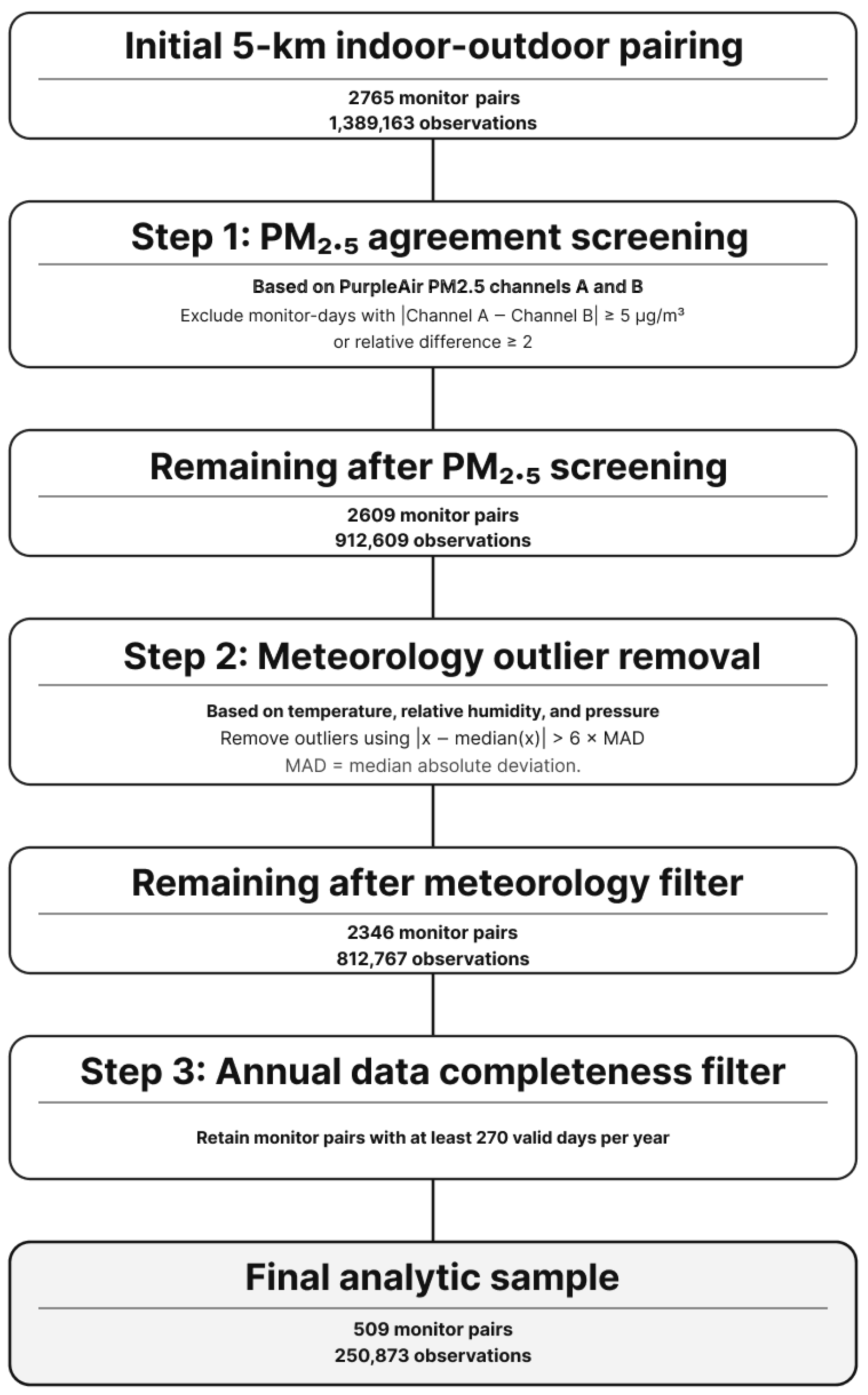
Figure 1 summarizes the data processing pipeline. We first formed 2765 indoor–outdoor monitor pairs within a 5 km buffer, yielding 1,389,163 daily paired observations. After applying CF1 channel-agreement quality control, removing meteorologic outliers in humidity, temperature, and pressure using a 6× MAD rule, and requiring at least 270 valid days per year for each pair, the analytic dataset included 509 unique indoor–outdoor pairs contributing 250,873 daily observations. Within-sensor agreement between CF1 channels was high among retained monitors (Pearson r: 0.97–1.00;
Supplementary Figure S1), supporting use of the channel-averaged PM
2.5 in subsequent analyses.
After all quality-control filters were applied, the number of paired monitors providing data increased from 22 in 2019 to 184 in 2024, with annual daily observations ranging from 6453 to 53,028 (
Table 1a). Of the monitors used in the analysis, 320 pairs (62.9%) contributed data for only one year, 112 (22%) for two years, and 45 (8.8%) for three years, whereas only 27 (5.3%) pairs contributed four years of data and 5 monitors (1%) contributed five years (
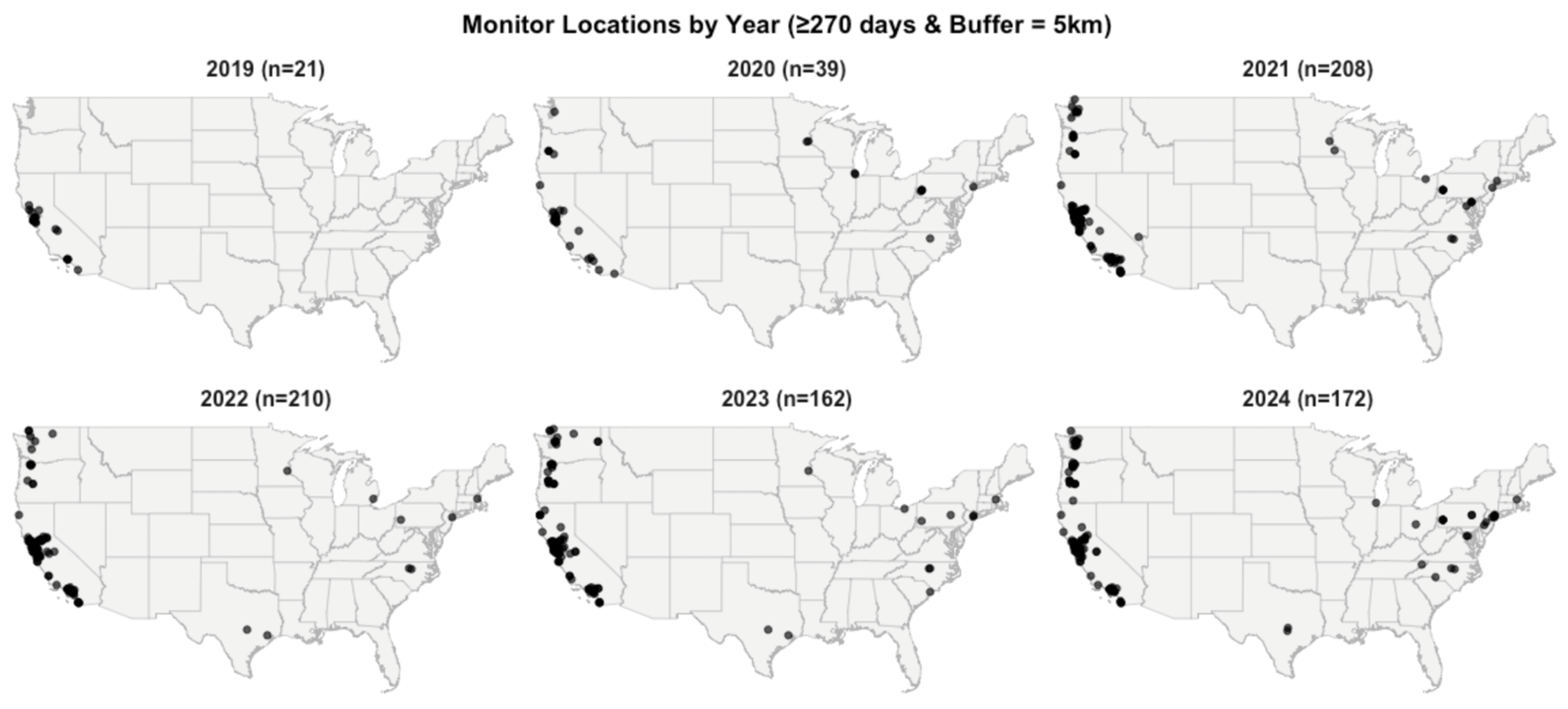
Table 1b). In 2019 and 2020, monitors were mostly located along the west coast, with clusters in coastal California and scattered sites in Washington, Oregon, and a few locations in the eastern United States (
Figure 2). Beginning in 2021, the network expanded substantially, with dense coverage throughout California and additional sites in the Southeast and Mid-Atlantic. The 2022–2024 panels show similar patterns, with the highest concentration of pairs in western states but increasing representation of eastern locations, spanning marine west-coast, Mediterranean, and humid continental to humid subtropical climate zones. Each dot represents one monitor pair contributing to the final analysis in that year.
Supplementary Figure S2 shows the geographic distribution of all unique monitors across U.S. climate regions. Among accepted indoor–outdoor pair-years, the pairing distance ranged from 0.000 to 4.822 km, with a median of 0.483 km and an interquartile range of 0.120 to 1.172 km. Most accepted pairs were substantially closer than the 5 km threshold, with 69.4% within 1 km and 85.6% within 2 km (
Supplementary Table S7). Among the 509 indoor sensors retained in the final analytic dataset, 43 (8.4%) had names suggestive of residential/private settings, 62 (12.2%) had clearly non-residential names, 76 (14.9%) used only generic indoor labels, and 328 (64.4%) had names that were too unclear to classify confidently (
Supplementary Table S8).
Smoke days exhibited substantially higher PM
2.5 both outdoors and indoors: mean outdoor PM
2.5 was 8.61 (SD 7.56) µg/m
3 on smoke days versus 5.63 (4.39) µg/m
3 on non-smoke days and mean indoor PM
2.5 was 6.33 (4.25) µg/m
3 versus 5.09 (3.21) µg/m
3 (both
p < 0.001) (
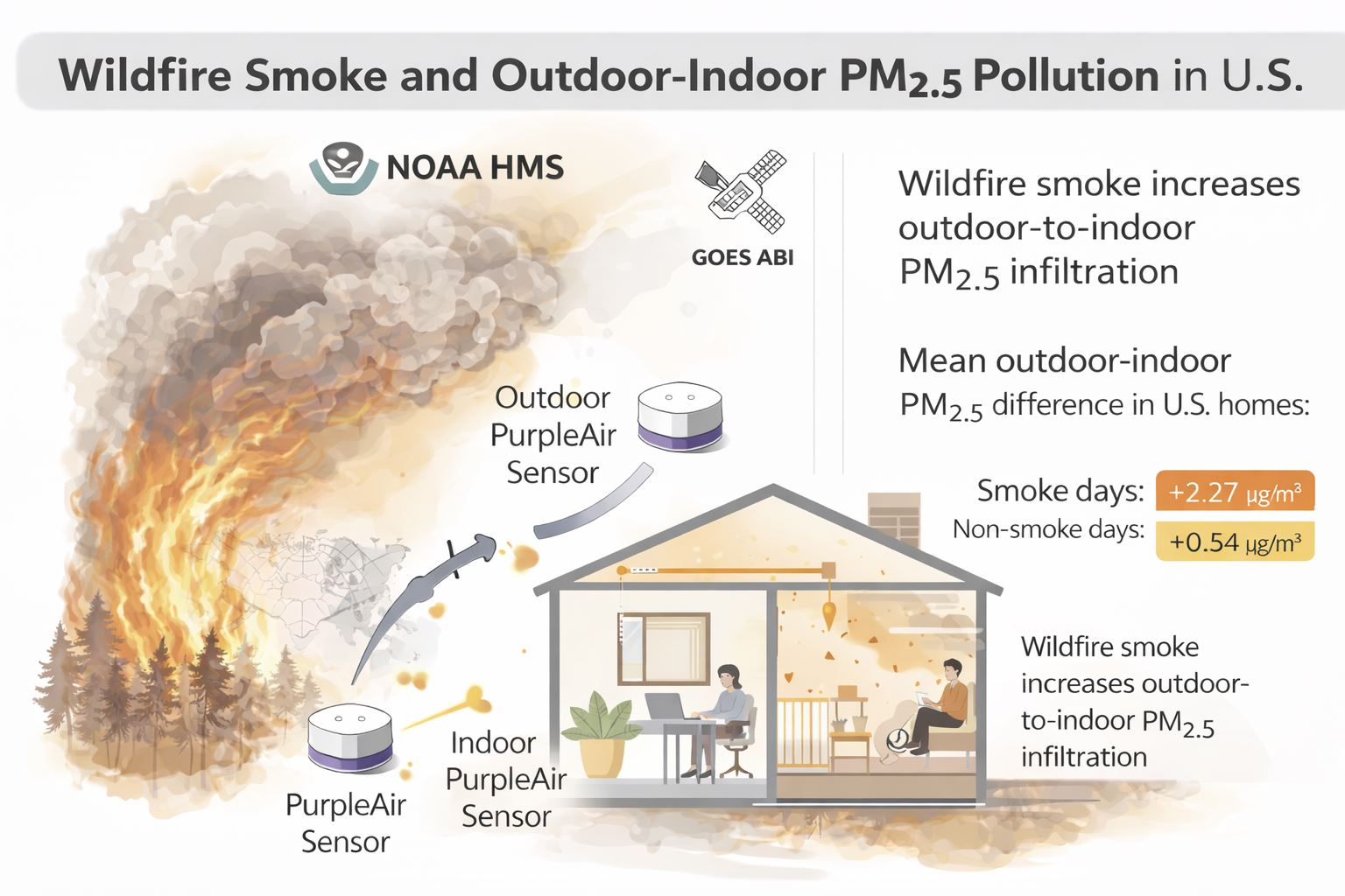
Table 2). Additionally, the outdoor–indoor difference increased from 0.54 (4.26) µg/m
3 on non-smoke days to 2.27 (6.16) µg/m
3 on smoke days (
p < 0.001). The median of the indoor/outdoor (I/O) ratios decreased from 0.97 (IQR: 0.72, 1.33) on non-smoke days to 0.83 (IQR: 0.61, 1.06) on smoke days (
p < 0.001). The meteorological conditions also differed significantly between smoke and non-smoke days: outdoor relative humidity was lower on smoke days, whereas indoor relative humidity was higher; both outdoor and indoor temperatures were higher on smoke days. These differences support the inclusion of temperature and relative humidity as covariates in the adjusted models.
As a supplementary paired nonparametric comparison, paired Wilcoxon signed-rank tests showed that outdoor PM
2.5 concentrations were significantly higher than indoor concentrations on both smoke days and non-smoke days (both
p < 2.2 × 10
−16). The estimated paired outdoor–indoor shift was larger on smoke days (pseudo-median shift = 1.460 µg/m
3, 95% CI: 1.428, 1.493) than on non-smoke days (pseudo-median shift = 0.265 µg/m
3, 95% CI: 0.255, 0.276), consistent with the main findings (
Supplementary Table S6).
Although the overall smoke-day mean outdoor PM
2.5 was modest, distributional summaries showed that smoke-day observations were consistently shifted upward relative to non-smoke days across the distribution. In
Supplementary Table S2, outdoor PM
2.5 on smoke days had higher median, 90th percentile (Q90), 95th percentile (Q95), and 99th percentile (Q99) values than on non-smoke days, and similar upward shifts were observed for indoor PM
2.5 and the outdoor minus indoor PM
2.5 difference.
Supplementary Figure S7 further shows that the smoke-day distribution includes a long upper tail of elevated concentrations despite the relatively modest overall mean. To further characterize this heterogeneity, we conducted an additional descriptive analysis (
Supplementary Table S5) focused on the upper tail of the smoke-day distribution. We defined high-smoke days as smoke-day observations with outdoor PM
2.5 at or above the smoke-day Q95 threshold. In this high-smoke subset, outdoor PM
2.5 was substantially more elevated than in the overall smoke-day sample, with a mean of 32.19 (15.62) µg/m
3, a median of 27.33 µg/m
3, a Q90 of 47.24 µg/m
3, a Q95 of 57.29 µg/m
3, a Q99 of 95.80 µg/m
3, and a maximum of 276.25 µg/m
3. Indoor PM
2.5 was also higher in this subset, with a mean of 14.36 µg/m
3 and a median of 12.16 µg/m
3, and the outdoor minus indoor PM
2.5 difference increased markedly, with a mean of 17.83 µg/m
3 and a median of 15.62 µg/m
3. These results indicate that the HMS-based smoke-day category encompasses a continuum of smoke influence, ranging from lower-intensity or transported smoke to substantially elevated smoke events.
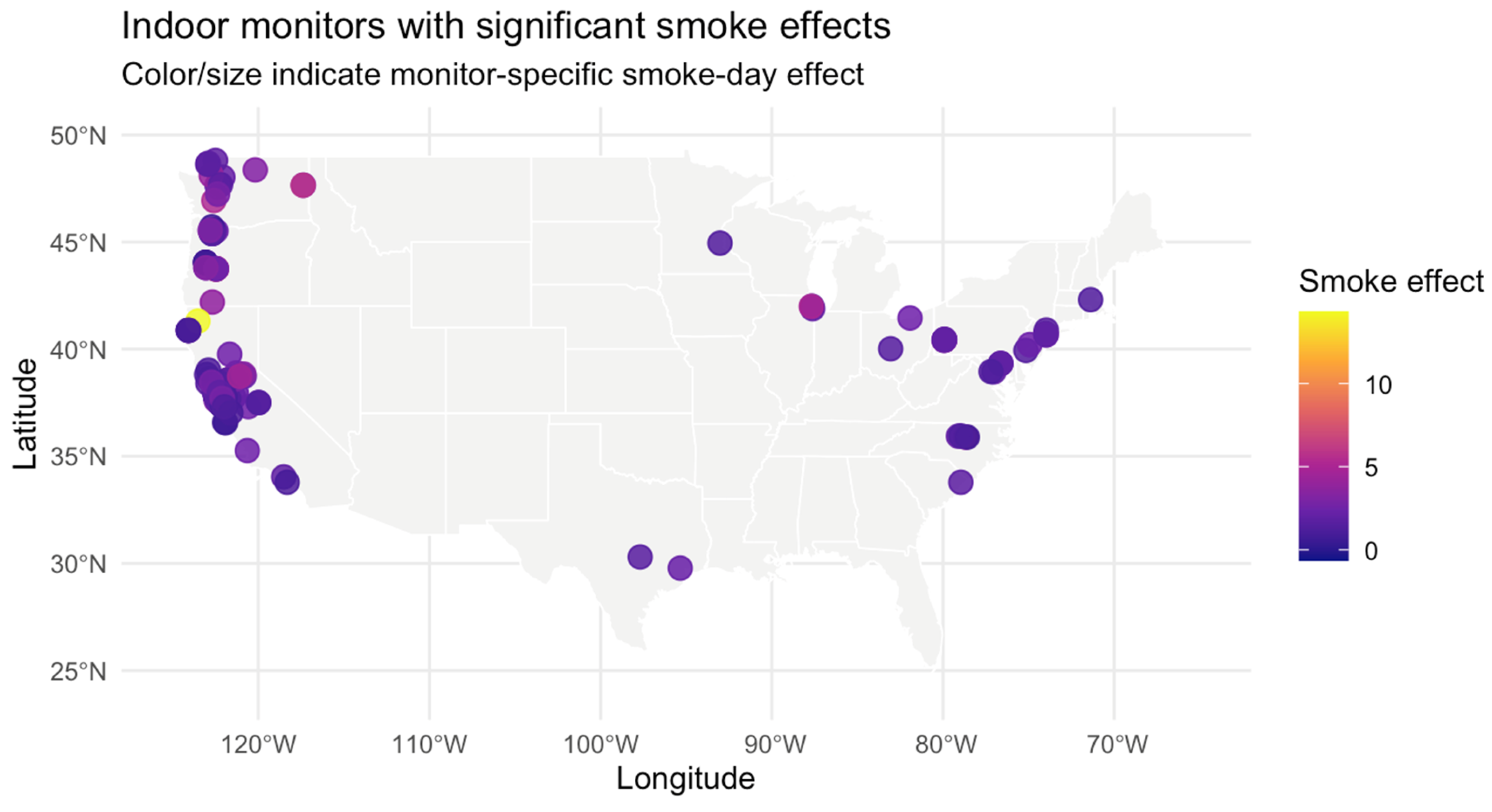
Figure 3 maps the mean significant smoke-day effect on the outdoor–indoor PM
2.5 difference across the United States. These significant smoke-day effects (N = 194) were obtained from the first-stage monitor-specific regression model adjusting for the temporal trends, humidity, and temperature. Nearly all occupied cells show positive effects, indicating that on smoke days outdoor PM
2.5 increased more than indoor PM
2.5 at most locations. The largest mean effects cluster along the west coast, especially in coastal California and the Pacific Northwest, where several grid cells exceed ~10 µg/m
3. Moderate positive effects are also evident in the Northeast and Mid-Atlantic corridor, while cells in the interior West and South show smaller but still generally positive smoke-day impacts. To enhance the visualization of spatial distribution, we divided the study area into a 40 by 40 grid, based on longitude and latitude. For each grid cell, we calculated the average smoke effect, and the color intensity in the heatmap represents the strength of the effect (
Supplementary Figure S3).
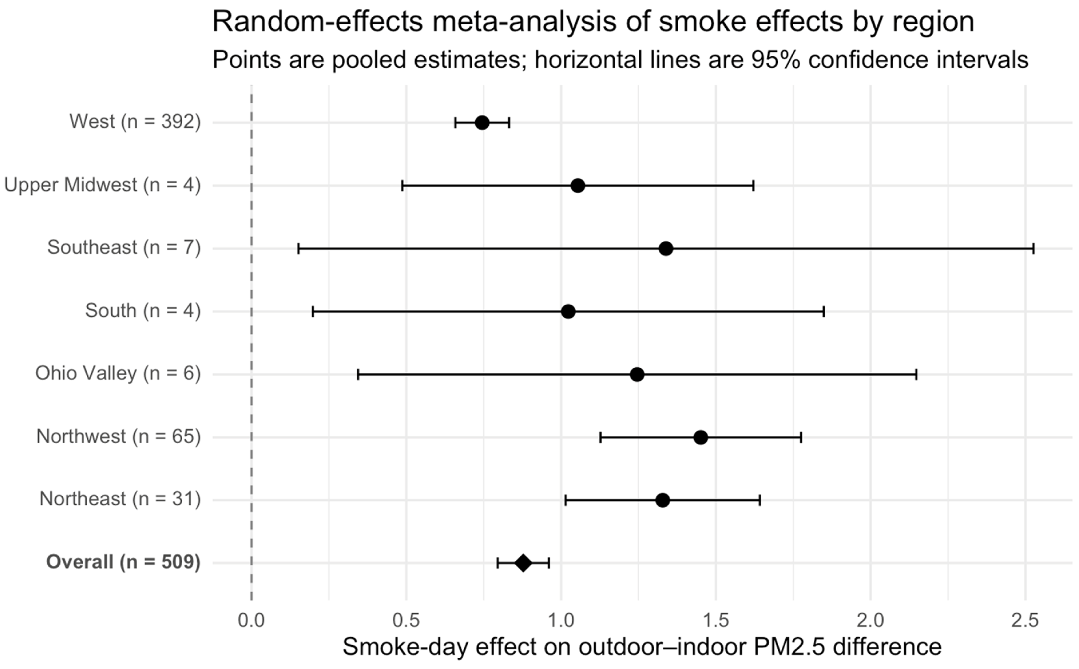
Figure 4 shows the smoke-day effects for all (N = 509) monitors, including those with non-significant first-stage estimates, using a random-effects meta-analysis stratified by geographic climate region. The pooled smoke-day effects on the outdoor–indoor PM
2.5 concentration difference (µg/m
3; 95% CI) were 1.45 µg/m
3 (1.13, 1.78) for the Northwest (n = 65), 0.72 µg/m
3 (0.66, 0.83) for the West (n = 392), 1.05 µg/m
3 (0.49, 1.62) for the Upper Midwest (n = 4), 1.25 µg/m
3 (0.34, 2.15) for Ohio Valley (n = 6), 1.02 µg/m
3 (0.20, 1.85) for the South (n = 4), 1.34 µg/m
3 (0.15, 2.53) for the Southeast (n = 7), and 1.33 µg/m
3 (1.01, 1.64) for the Northeast (n = 31). The overall pooled effect across all monitors is 0.88 µg/m
3 (95% CI: 0.80, 0.96). Numerical values corresponding to
Figure 4 are provided in
Supplementary Table S1.
Table 3 shows the clustering results across 472 monitor pairs that showed increased outdoor PM
2.5 on smoke days. Four distinct patterns of indoor–outdoor PM
2.5 response during smoke days were grouped. The most common pattern, low outdoor increase, strong indoor attenuation (Cluster A; n = 224, 47.5%), was characterized by relatively small outdoor PM
2.5 increases (mean d_out = 1.60 μg/m
3, SD: 0.68) and even smaller indoor increases (mean d_in = 0.84 μg/m
3, 0.57). A second group, moderate outdoor increase, partial indoor attenuation (Cluster B; n = 167, 35.3%), exhibited larger outdoor PM
2.5 increases (mean d_out = 4.04 μg/m
3, SD: 1.31) accompanied by appreciable indoor increases (mean d_in = 1.89 μg/m
3, SD: 1.17), reflecting incomplete attenuation and substantial indoor exposure during smoke events. A small subset of locations fell into an extreme outdoor amplification pattern (Cluster C; n = 12, 2.5%), with very large outdoor PM
2.5 increases (mean d_out = 11.91 μg/m
3, SD: 7.24) and correspondingly elevated but variable indoor responses (mean d_in = 4.83 μg/m
3, SD: 3.96). Notably, a fourth pattern emerged in which indoor PM
2.5 concentrations decreased during smoke days relative to non-smoke days (indoor reduction during smoke events; Cluster D; n = 69, 14.6%). Despite modest outdoor PM
2.5 increases (mean d_out = 1.75 μg/m
3, SD: 1.25), these monitors exhibited negative indoor changes (mean d_in = −0.60 μg/m
3, SD: 0.62).
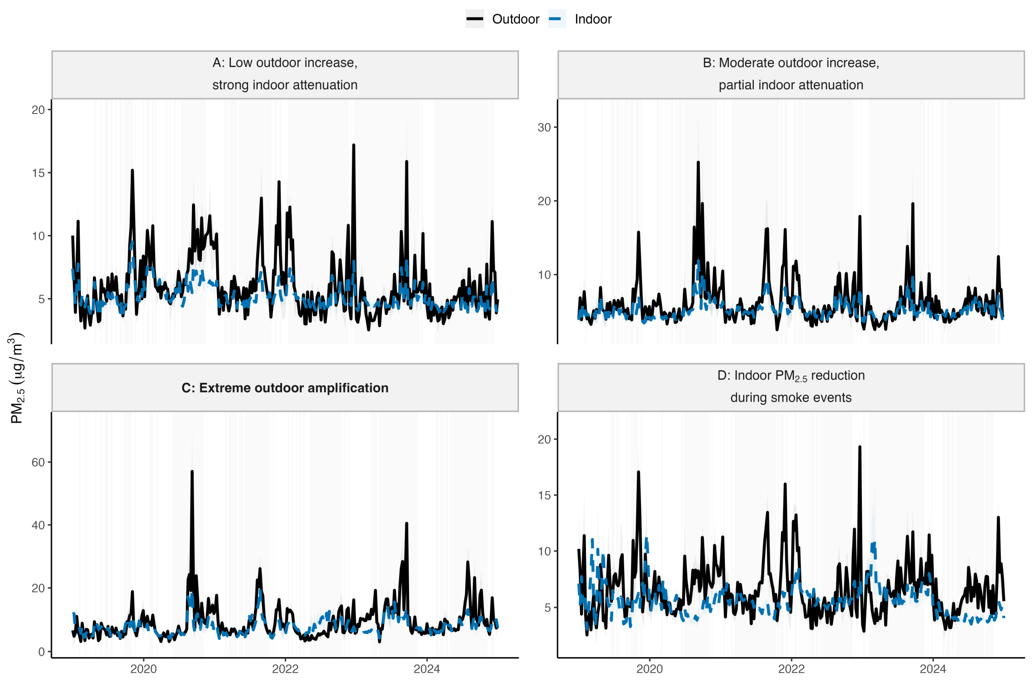
For visualization in
Figure 5, we aggregated the indoor and outdoor PM
2.5 time series to weekly means within each cluster and overlaid a smoothed trend; gray shading denotes weeks containing at least one smoke day.
Figure 5 shows a clear gradient in smoke-related outdoor excursions across clusters, with progressively larger outdoor peaks from Clusters A to C. Indoor PM
2.5 generally tracks these outdoor increases but with attenuated magnitude in Clusters A–C, whereas Cluster D departs from this pattern and shows lower indoor PM
2.5 during smoke weeks despite concurrent outdoor increases.
In the
–
plane (
Supplementary Figure S4), the clusters formed a continuous gradient rather than sharply separated groups. Outdoor amplification increased along the horizontal axis, while indoor attenuation decreased along the vertical axis. Notably, Cluster D (green dots, the PM
2.5 concentrations decreased during smoke days) was confined to the far left of the plot, indicating consistently low outdoor PM
2.5 increases on smoke days.
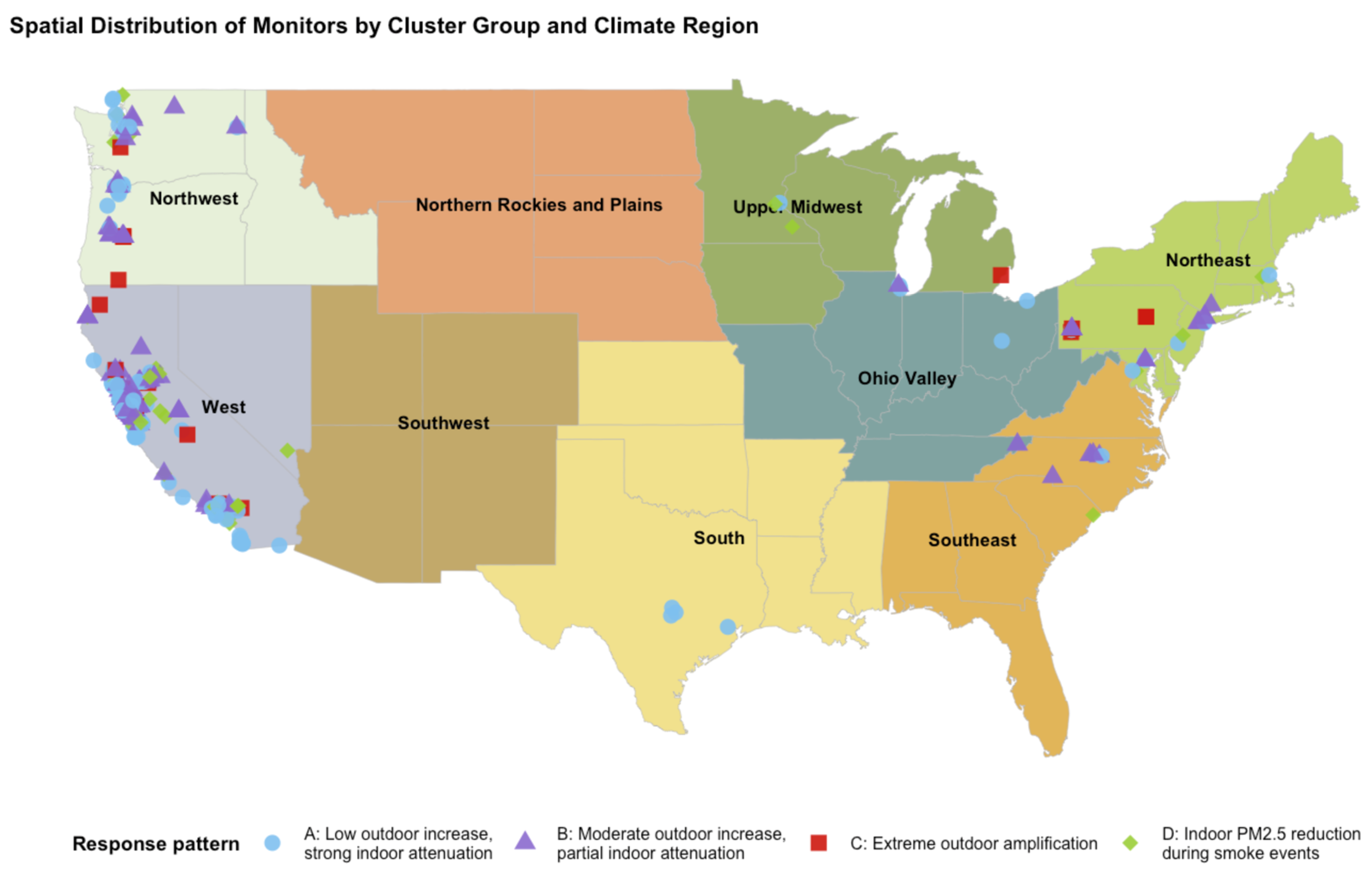
Figure 6 displays the geographic distribution of monitoring locations by outdoor–indoor PM
2.5 response pattern overlaid on U.S. climate regions. Overall, response patterns were spatially heterogeneous but exhibited clear regional tendencies. Monitors classified as low outdoor increase with strong indoor attenuation (Cluster A) and moderate outdoor increase with partial indoor attenuation (Cluster B) were widely distributed across the United States and represented the dominant response patterns in most climate regions. Locations exhibiting extreme outdoor amplification (Cluster C) were rare and geographically concentrated, appearing primarily in the western United States, including the West and Northwest climate regions. These sites coincided with regions more frequently affected by intense wildfire smoke episodes, consistent with the large outdoor PM
2.5 increases observed for this cluster. Similarly, monitors classified as indoor PM
2.5 reduction during smoke events (Cluster D) were scattered primarily in the West regions, with smaller numbers in the Upper Midwest, Northeast, and Southeast regions.
4. Discussion
4.1. Outdoor–Indoor PM2.5 Differences Increase During Smoke Days
In unadjusted comparisons (two-sample t-tests), smoke days had higher outdoor PM2.5, higher indoor PM2.5, and a larger outdoor–indoor difference than non-smoke days. Site-specific linear models that controlled for temperature and humidity produced mostly positive smoke-day coefficients, and the primary overall random-effects meta-analysis across all monitored sites showed a positive association between smoke days and the outdoor–indoor PM2.5 difference. Region-stratified estimates were also generally positive, but these were intended as secondary descriptive summaries of geographic heterogeneity and should be interpreted cautiously in sparsely sampled regions. Regional analyses suggested that the smoke-day effect on the outdoor–indoor PM2.5 difference was positive overall and generally positive across regions, although precision varied substantially because monitor coverage was highly uneven. Estimates were most stable in the West and Northwest, where monitor density was greatest, whereas several other regions had much wider confidence intervals due to sparse representation.
These patterns align with prior reports showing that wildfire episodes substantially elevate outdoor concentrations while buildings provide only partial attenuation. Studies using both crowdsourced and targeted field monitors have documented sharp increases in outdoor PM
2.5 on smoke days, with indoor concentrations rising as well but remaining well below outdoor levels because only a fraction of outdoor smoke penetrates indoors [
24,
25,
26,
49]. These studies also report lower I/O ratios and reduced infiltration factors during smoke events, which aligns with our observation that the I/O ratios were lower on smoke days compared with non-smoke days.
Comparison with studies from other geographical regions supports the broader relevance of our findings. In Australia, wildfire smoke has been shown to contribute substantially to ambient PM
2.5 during fire seasons, with especially strong impacts during severe years in southeastern cities, while plume studies in New South Wales [
50] indicate that not all mapped smoke plumes produce strong surface PM
2.5 enhancement because some smoke remains aloft. In Europe, both local wildfire episodes, such as the 2017 Portuguese fires, and long-range transport events, such as smoke from the 2023 Canadian wildfires, have been linked to elevated PM
2.5 and degraded air quality [
51,
52]. Together, these studies suggest that our results fit a broader international pattern in which wildfire emissions consistently increase outdoor PM
2.5, but the observed magnitude varies with fire intensity, transport distance, plume injection height, and meteorological conditions [
41]. This also helps explain why our HMS-based multi-region analysis captured a wide range of smoke conditions, including lower-intensity and transported-smoke days, rather than only severe near-source wildfire episodes.
However, the overall mean concentration on smoke days should be interpreted cautiously. Because smoke days were defined using a binary HMS plume-overlap indicator, this category captures a broad spectrum of smoke influence, including dilute transported smoke, moderate smoke conditions, and a smaller number of substantially elevated episodes, rather than isolating only severe wildfire events. This interpretation is supported by the new supplementary distributional analyses.
Supplementary Table S2 shows that the smoke-day distribution is shifted upward relative to the non-smoke-day distribution across the median and upper quantiles, and
Supplementary Figure S7 shows that smoke days include a long upper tail of relatively high concentrations. In addition,
Supplementary Table S5 demonstrates that smoke-day observations at or above the smoke-day Q95 threshold had much higher outdoor and indoor PM
2.5 concentrations than the overall smoke-day average. Taken together, these results indicate that the relatively modest mean outdoor PM
2.5 on all smoke days reflects averaging across a heterogeneous distribution, rather than the absence of meaningful smoke episodes.
To move beyond the overall upward shift in outdoor–indoor PM2.5 during smoke days, we next used a clustering approach to identify four distinct patterns of smoke-day outdoor and indoor PM2.5 changes.
4.2. Outdoor Amplification Is the Dominant Driver; Indoor Responses Modulate How Wide the Gap Becomes
The clustering results show that smoke-day changes in the outdoor–indoor PM
2.5 gap are not a single uniform pattern but instead fall into four consistent response modes. Across clusters, the dominant feature is outdoor amplification: outdoor PM
2.5 increases are consistently larger and more variable than indoor changes, helping explain the overall reduction in the I/O ratio on smoke days. The clusters further indicate that indoor PM
2.5 does not respond uniformly to outdoor smoke. Three clusters (
Supplementary Figure S4) span a spectrum from relatively modest to extreme smoke impacts, in which indoor PM
2.5 generally increases but less than outdoors, consistent with partial indoor tracking whose strength varies across conditions. In contrast, the fourth cluster is qualitatively distinct, characterized by smoke-day decreases in indoor PM
2.5 despite outdoor increases, indicating a weakly coupled indoor response that can offset or even reverse the expected indoor elevation during smoke events.
Interpretively, the clusters provide a data-driven typology that separates the magnitude of the smoke-day outdoor PM2.5 increase from the magnitude and direction of the corresponding indoor PM2.5 change. In this framework, monitor pairs are distinguished by whether smoke days are characterized by relatively small, moderate, or extreme outdoor PM2.5 increases, and by whether indoor PM2.5 increases only slightly, increases substantially but less than outdoors, remains near baseline, or decreases. This distinction shows that a larger outdoor–indoor PM2.5 contrast can arise under multiple indoor response patterns, even when outdoor smoke is present in all settings. Thus, the public-health relevance of a smoke day depends not only on the severity of outdoor smoke, but also on how strongly indoor concentrations rise or are attenuated relative to that outdoor increase. In the following sections, we describe each cluster’s characteristic smoke-day signature and its implications for indoor exposure during wildfire smoke events.
4.3. Cluster A and D: Small Outdoor Increases with Contrasting Indoor Response
Cluster A and Cluster D both occur under smoke episodes with relatively small outdoor PM2.5 increases, but they differ markedly in indoor response. This contrast shows that similar outdoor smoke conditions do not necessarily produce similar indoor PM2.5 changes. Under modest outdoor smoke conditions, variability in indoor response becomes especially apparent, ranging from slight indoor increases (Cluster A) to net indoor decreases (Cluster D).
Cluster A represents a “dampened increase” regime, where outdoor PM
2.5 rises on smoke days but indoor PM
2.5 increases only slightly. This pattern is consistent with limited net particle entry and/or effective indoor removal during modest smoke loading. Although the present analysis does not directly identify mechanisms, possible contributors include reduced particle penetration associated with lower air exchange rates, or more effective indoor particle removal. Prior studies suggest that tighter building envelopes, reduced outdoor air intake, and filtration can all reduce the rate at which outdoor particles contribute to indoor concentrations [
24,
29]. In addition, indoor concentrations may remain near baseline when filtration and deposition remove particles at a rate comparable to or greater than the incoming particle load [
31,
53]. Thus, Cluster A likely reflects settings in which outdoor smoke influences indoor air quality, but that influence is substantially damped.
Cluster D is qualitatively distinct because indoor PM
2.5 decreases on smoke days even as outdoor PM
2.5 increases. This pattern suggests that the net indoor PM
2.5 change reflects the combined effects of outdoor infiltration, indoor removal, and indoor source dynamics, rather than outdoor smoke alone [
54]. One plausible pathway is that when outdoor smoke increases are modest, reduced indoor particle generation or stronger indoor removal can outweigh the additional outdoor contribution. Previous work suggests that indoor PM
2.5 can be shaped by household activities, source control, filtration, and ventilation behaviors during smoke events [
55,
56]. For example, some households may respond to smoke by increasing filtration (operating portable air cleaners or running HVAC fans continuously) to minimize outdoor air intake. If removal increases and air exchange decreases sufficiently, indoor PM
2.5 can drop below its typical level [
24,
31]. However, because our analysis does not include household-level information such as filtration use, occupancy, cooking, or HVAC operation, Cluster D should be interpreted cautiously as an empirical response pattern rather than evidence for any single mechanism. In addition, given the broader HMS-based smoke-day definition used in this study, Cluster D is best understood as a pattern arising primarily under relatively modest smoke-related outdoor increases, rather than as evidence of indoor protection during severe wildfire smoke episodes.
Geographically, Cluster A was observed across multiple regions, including the West and parts of the East, indicating that this damped indoor response is not limited to the most smoke-affected areas. In contrast, Cluster D was more concentrated in California and the western U.S., with fewer sites elsewhere. One possible explanation is that California and other western regions experience wildfire smoke more frequently and intensely than most other parts of the U.S., which may increase the likelihood that households adopt protective behaviors or use filtration during smoke episodes. However, because the present study did not directly measure mitigation practices or housing characteristics, this interpretation remains speculative. Overall, the contrast between Clusters A and D highlights that even under relatively small outdoor smoke increases, indoor responses can vary substantially across settings.
4.4. Cluster B: Moderate Outdoor Increase with Partial Indoor Attenuation
Cluster B represents a common and policy-relevant regime in which outdoor PM
2.5 increases during smoke episodes are large enough to produce a clear indoor response, yet indoor concentrations remain lower than outdoors. In
Figure 5B, indoor and outdoor trajectories rise and fall together over extended smoke-week intervals, indicating that indoor air quality is meaningfully influenced by outdoor smoke under these conditions. This co-movement implies partial attenuation rather than full protection: staying indoors reduces exposure relative to outdoors, but it does not prevent indoor PM
2.5 from reaching elevated levels during smoke episodes. In practice, Cluster B is the scenario where the public message “stay indoors” is directionally correct but may be insufficient by itself, because a large fraction of homes can still experience appreciable indoor degradation even when outdoor increases are not extreme.
A parsimonious explanation for Cluster B is that outdoor particle entry remains substantial while indoor removal is not strong enough to offset the incoming load. Possible contributors include building leakage, door opening, and ventilation operation that admits outdoor air [
24], as well as limited filtration effectiveness relative to event intensity [
31]. These factors are not mutually exclusive, and together they can produce the observed pattern of indoor increases that lag only slightly behind outdoor changes and remain persistently elevated during smoke-week periods. Indoor activities may also contribute, since greater time spent indoors during smoke events can increase particle generation or resuspension. When people stay indoors more, indoor particle generation can increase through cooking and other activities, and resuspension can rise with occupancy [
55,
57].
Cluster B appears in both the western U.S. and multiple eastern locations, indicating that the moderate-outdoor-increase, partial-indoor-attenuation regime is not confined to a single region. This broad distribution suggests that partial indoor attenuation under moderate smoke can arise across a wide range of building types, climates, and household conditions.
4.5. Cluster C: Extreme Outdoor Amplification with Elevated but Variable Indoor Response
Cluster C captures rarer but high-impact episodes characterized by very large outdoor PM
2.5 increases and substantial indoor elevations. In
Figure 5C, this mode stands out not only for higher outdoor peaks but also for longer intervals of elevated concentrations, with indoor PM
2.5 remaining high across smoke-week periods rather than showing only brief excursions. This sustained elevation indicates that extreme events can move indoor air from “lower than outdoors” to “still high enough to be concerning,” especially when high outdoor loading persists for multiple days.
Mechanistically, Cluster C is consistent with a nonlinear exposure dynamic: even if the fraction of outdoor particles that enter indoors is reduced, very high outdoor concentrations can still yield large indoor burdens because the absolute amount entering remains large [
24]. Prolonged outdoor loading further increases the likelihood of indoor accumulation, since indoor PM
2.5 reflects the balance between continuous entry and removal processes that operate over time [
58,
59]. When outdoor concentrations remain high for days, indoor removal by filtration, deposition, and air exchange may not be sufficient to quickly return indoor levels to baseline, producing a raised indoor plateau and slower recovery. The variability in indoor response within Cluster C is also expected. Differences in housing tightness, filtration capacity, HVAC operation, and occupant mitigation behavior can produce substantial between-home heterogeneity even under similarly severe outdoor conditions, which aligns with the wider spread of indoor values in this cluster. It is also plausible that extreme events trigger sustained time indoors and behavior changes that can either reduce infiltration (for example closing windows) or increase indoor sources (for example more cooking), and the net effect may differ by household [
24,
29].
Geographically, Cluster C is much less prevalent and is concentrated primarily in the western U.S., with only a small number of sites outside the West. This spatial pattern is consistent with Cluster C, representing high-severity episodes that occur more often where intense smoke events are more common, while also indicating that severe impacts can occur outside the West within this monitoring network. Geographic patterns should be interpreted alongside monitoring density, which is higher in parts of the West and may influence the apparent distribution of sites.
4.6. Public Health Implications
These findings imply that a “smoke day” should not be treated as a single indoor exposure condition. Being indoors typically leads to reduced exposures compared to corresponding estimates of exposure based on outdoor concentrations, but indoor PM
2.5 often increases during smoke episodes, and this can occur even when outdoor smoke levels are only small-to-moderate. Public guidance should therefore avoid implying that staying indoors alone is sufficient, and should pair location-based advice with clear, actionable steps that reduce indoor particle levels, including continuous filtration, minimizing outdoor air entry when feasible, and avoiding indoor particle-generating activities during smoky periods. At the same time, the observed instances of indoor PM
2.5 reductions during small outdoor smoke increases indicate that timely and sustained mitigation can meaningfully change indoor conditions, supporting early action rather than waiting until smoke becomes severe. Because we lack household-level information on behaviors and building operation, this pattern should be interpreted as evidence of potential, rather than as attribution to any specific action. Finally, the most intense smoke episodes were associated with sharp and persistent indoor elevations, underscoring the importance of escalation strategies during severe events, including approaches that increase effective particle removal and provide access to cleaner indoor environments for households unable to maintain adequate indoor air quality at home. Future work incorporating neighborhood socioeconomic context, housing characteristics, and more standardized information on building type and indoor setting could help explain heterogeneity in smoke-related indoor PM
2.5 responses and identify which communities are most vulnerable to higher indoor smoke exposure, consistent with prior evidence [
60] that county-level socioeconomic and environmental factors contribute to spatial heterogeneity in health burden. Future work linking sensor data with time-resolved mitigation behaviors, such as HVAC operation, portable air cleaner use, and window-opening patterns, could help identify which actions most effectively reduce indoor PM
2.5 during smoke events and strengthen behavior-specific public health guidance.
4.7. Strengths and Limitations
This study has several strengths. First, we leveraged paired indoor and nearby outdoor PurpleAir sensors across multiple seasons, years, and U.S. regions, yielding a large, high-time-resolution dataset for characterizing indoor–outdoor relationships during wildfire smoke events. Second, we applied a two-stage analytic framework that adjusted for meteorology (temperature and humidity) and temporal trends to reduce confounding by seasonal cycles and weather-related co-variation with smoke. This approach estimated site-specific associations and then synthesized them using random-effects meta-analysis, explicitly accounting for between-site heterogeneity. Third, we introduced a quantitative clustering approach that provides a principled summary of heterogeneity in indoor responses. Together, these elements extend prior field and crowdsourced studies, which often focus on single regions or one to two fire seasons, by demonstrating consistent qualitative patterns in a multi-region dataset spanning five years while also identifying structured, interpretable variation in indoor exposure dynamics across climates, housing contexts, and smoke intensities.
Important limitations should also be acknowledged. The PurpleAir network is crowdsourced, so homes with monitors are not representative of the full housing stock; participants may have higher socioeconomic status, greater environmental awareness, or greater access to filtration. After applying quality-control and completeness criteria, the analytic sample also remained geographically imbalanced, with most monitor pairs located in the West and Northwest and under-representation of several other U.S. climate regions. Because indoor and outdoor monitors were paired within 5 km rather than treated as strictly co-located, some local-scale spatial mismatch may remain, particularly from non-smoke background PM2.5 sources. In addition, we lack detailed information on building characteristics (e.g., year built, envelope tightness, HVAC type), filter ratings and maintenance, and time-resolved occupant behaviors (e.g., window opening, HEPA use, cooking patterns), which limits our ability to explain heterogeneity or to estimate the effects of specific mitigation measures. Smoke-day classification based on satellite-derived HMS plume products may also misclassify some days, particularly when smoke is thin, patchy, obscured by clouds, or remains aloft without strongly affecting ground-level PM2.5 at a given location. Although our supplementary descriptive analyses showed that outdoor PM2.5 distributions on HMS-classified smoke days were consistently shifted upward relative to non-smoke days, supporting a meaningful surface smoke signal overall at the daily scale, the binary HMS-based definition likely still combines a range of smoke conditions, from diffuse transported smoke to more elevated smoke episodes. Together, these limitations likely introduce extra variability and could either attenuate or amplify site-specific effects depending on local conditions.