A Hybrid Digital CO₂ Emission-Control Technology for Maritime Transport: Physics-Informed Adaptive Speed Optimization on Fixed Routes

Abstract

This paper proposes a physics-informed hybrid digital CO₂ emission-control technology for maritime transport, designed for adaptive ship speed optimization along a predefined geographical route between two ports, discretized into quasi-stationary segments and evaluated under forecasted metocean conditions, subject to economic and regulatory constraints associated with maritime decarbonization. The framework integrates two exact optimization methods, Backtracking (BT) and Dynamic Programming (DP), with a reinforcement learning approach based on Proximal Policy Optimization (PPO), operating on a unified physical, economic, and regulatory modeling core. By reducing propulsion fuel demand, the system acts as an upstream CO₂ emission-control mechanism for ship propulsion. This operational stabilization of the engine load creates favourable boundary conditions for advanced combustion processes and reduces the volumetric flow of exhaust gas, thereby lowering the technical burden on potential post-combustion carbon capture systems. Segment-wise speed profiles are optimized subject to propulsion limits, Estimated Time of Arrival (ETA) feasibility, and regulatory constraints, including the Carbon Intensity Indicator (CII), the European Union Emissions Trading System (EU ETS) and FuelEU Maritime. The physics-based propulsion and energy model is validated using full-scale operational data from four real voyages of an oil/chemical tanker. A detailed case study on the Milazzo–Motril route demonstrates that adaptive speed optimization consistently outperforms conventional cruise operation. Exact optimization methods achieve voyage time reductions of approximately 10% and fuel and CO₂ emission reductions of about 9–10%. The reinforcement learning approach provides the best overall performance, reducing voyage time by approximately 15% and achieving fuel savings and CO₂ emission reductions of about 13%. At the route level, the Carbon Intensity Indicator is reduced by approximately 10% for the exact methods and by about 13% for PPO. Backtracking and Dynamic Programming converge to nearly identical globally optimal solutions within the discretized decision space, while PPO identifies solutions located on the most favourable region of the cost–time Pareto front. By benchmarking reinforcement learning against exact discrete solvers within a shared physics-informed structure, the proposed digital platform provides transparent validation of learning-based optimization and offers a scalable decision-support technology for pre-fixture evaluation of fixed-route voyages. The system enables quantitative assessment of CO₂ emissions, ETA feasibility, and regulatory exposure (CII, EU ETS, FuelEU Maritime penalties) prior to transport contracting, thereby supporting economically and environmentally informed operational decisions.

1. Introduction

Maritime transport operates under an increasingly stringent regulatory framework [1] aimed at controlling atmospheric emissions arising from fuel combustion. Traditionally, air pollutants such as nitrogen oxides (NO_x), sulphur oxides (SO_x), and particulate matter have been mitigated through combustion-related and post-combustion technologies, including Selective Catalytic Reduction (SCR), exhaust gas cleaning systems (scrubbers), and the use of low-sulphur or alternative fuels, in accordance with MARPOL Annex VI requirements [2]. These measures have proven effective in limiting conventional pollutants and are widely implemented across the global fleet.

Carbon dioxide (CO₂) emissions, however, differ fundamentally from other exhaust pollutants. Since CO₂ formation is directly proportional to fuel consumption and carbon content, its mitigation cannot rely solely on after-treatment technologies and instead requires a reduction in fuel use at the source. Although onboard carbon capture systems are currently under pilot development, they are not yet widely deployed in commercial shipping [3]. Consequently, operational fuel-consumption reduction remains the primary immediately deployable strategy for CO₂ mitigation. This operational control principle is explicitly embedded in major regulatory instruments, including the IMO Carbon Intensity Indicator (CII) [4,5], the inclusion of maritime transport in the EU Emissions Trading System (EU ETS) [6,7] and the FuelEU Maritime regulation [8], all of which explicitly link operational performance to CO₂ exposure and economic liability.

The proportional relationship between fuel consumption and CO₂ emissions is well established in the IMO Fourth GHG Study 2020 [9] and related assessments of maritime decarbonization pathways. Because the main propulsion engine represents the dominant onboard emission source in ocean-going vessels, reducing fuel flow proportionally decreases the total exhaust mass flow and thus reduces not only CO₂ but also combustion-related pollutants such as NO_x, SO_x, and particulate matter, whose emission rates are strongly correlated with engine load and fuel throughput [2,9]. Accordingly, operational optimization strategies function as upstream emission-control mechanisms that complement combustion and after-treatment technologies. By reducing fuel demand at source, such strategies effectively moderate the intensity of onboard combustion processes and the associated formation of combustion-derived pollutants.

Within this regulatory and technological context, voyage speed optimization has emerged as a first-order operational CO₂ control approach. Vessel speed strongly influences propulsion power demand through nonlinear hydrodynamic resistance relationships, leading to significant variation in fuel consumption and associated emissions. Classical analyses demonstrated the strong cubic-type dependency between speed and required propulsion power, providing the theoretical foundation for modern speed-optimization models [10]. Unlike hardware retrofits or fuel switching, speed optimization can be implemented immediately across existing fleets without capital modification, making it particularly attractive under tightening regulatory constraints.

However, conventional constant-speed or real-speed cruise planning neglects spatial variability in environmental conditions such as currents, wind, and waves. These metocean factors introduce segment-wise heterogeneity in propulsion power demand and emissions, rendering uniform speed selection suboptimal from both energy-efficiency and emission-control perspectives. Addressing this limitation requires a modeling and optimization framework capable of capturing segment-level physical effects while remaining consistent with regulatory and economic constraints.

In this study, we propose a physics-informed hybrid optimization framework for fixed-route voyage speed control explicitly targeting CO₂ emission reduction through operational optimization. A predefined geographical route—defined by known waypoints between two ports—is discretized into quasi-stationary segments characterized by distance and environmental inputs. Segment-wise speeds are optimized using a unified modeling core that integrates the following:

(i)

Physics-based propulsion power, fuel consumption, and CO₂ emission estimation grounded in naval architecture practice and validated against full-scale operational data [9];

(ii)

Exact discrete optimization methods (Backtracking and Dynamic Programming) providing global optimality guarantees within the discretized decision space [11,12];

(iii)

A reinforcement learning approach based on Proximal Policy Optimization (PPO), designed to learn adaptive speed-selection policies under identical physical and regulatory constraints [13].

Beyond the methodological formulation, the proposed framework has been implemented as a fully operational digital CO₂ emission-control technology integrated into a dedicated voyage optimization software platform, applicable to existing fleets without hardware retrofits. The developed application integrates the calibrated physics-based propulsion model, the exact optimization solvers, and the reinforcement learning module within a unified computational architecture. It enables segment-wise speed control under real regulatory constraints and provides transparent outputs, including fuel consumption, CO₂ emissions, CII values, ETA compliance, and economic exposure. The contribution of this study, therefore, extends beyond theoretical modeling to a deployable digital emission-control solution for maritime propulsion systems.

The fixed-route assumption reflects practical operational contexts, including pre-fixture planning, contractual ETA evaluation, regulatory compliance assessment (CII, EU ETS, FuelEU Maritime), and speed adjustment along established shipping lanes. The framework is not intended to replace dynamic weather-routing systems that optimize route geometry in real time; rather, it complements them by providing a high-fidelity operational CO₂ control layer along a predefined route under known or forecasted environmental conditions.

The main contributions of this work are as follows:

• A calibrated, physics-informed per-segment propulsion and emission model validated against full-scale operational data;
• Two exact discrete optimizers serving as globally optimal reference solvers;
• A PPO-based reinforcement learning agent trained within the same physics-informed environment;
• A unified constraint-handling structure enabling consistent treatment of ETA feasibility, CII limits, and regulatory costs.

By positioning operational speed optimization as a practical and immediately deployable CO₂ emission-control technology, complementary to combustion, fuel, and emerging capture-based measures, the proposed framework contributes to the broader objective of pollution control and maritime decarbonization.

The remainder of the paper is organized as follows: Section 2 reviews the relevant literature; Section 3 presents the methodology; Section 4 describes the software implementation; Section 5 details calibration and validation; Section 6 presents the case study results; Section 7 concludes the paper.

2. Literature Review and Theoretical Background

2.1. Economic and Environmental Integration

Recent regulatory developments have transformed operational CO₂ emissions from a purely environmental metric into a direct economic variable in maritime transport. The introduction of the Carbon Intensity Indicator (CII) under IMO guidelines [4,5] establishes annual efficiency ratings linked to operational carbon intensity, while the inclusion of maritime transport in the EU Emissions Trading System (EU ETS) [6,7] directly monetizes CO₂ emissions through mandatory allowance purchases. Under the EU ETS framework, ship operators must acquire emission allowances proportional to verified CO₂ output, with market-based price signals provided by exchanges such as EEX and S&P Global [14,15]. As of 2024, ETS applies fully to intra-EU voyages and partially to international voyages involving EU ports, increasing the financial sensitivity of operational speed decisions.

FuelEU Maritime (Regulation EU 2023/1805) [8] complements the ETS mechanism by imposing progressively stricter limits on the well-to-wake greenhouse gas (GHG) intensity of onboard energy use. Unlike ETS, which prices emissions ex post, FuelEU establishes compliance thresholds, with non-compliance triggering penalties proportional to excess GHG intensity. Together with CII rating requirements, these instruments create a coupled regulatory–economic environment in which voyage speed simultaneously influences fuel consumption, emissions exposure, compliance risk, and operational cost.

Consequently, contemporary voyage optimization models increasingly adopt integrated cost formulations that jointly represent fuel expenditure, charter-time implications, emissions pricing, and regulatory penalties. Such formulations enable multi-objective trade-off analysis between schedule reliability, energy efficiency, and compliance under evolving decarbonization frameworks.

2.2. Theoretical Basis of Speed Optimization

The theoretical foundation of ship speed optimization is rooted in the nonlinear relationship between vessel speed, propulsion power, and fuel consumption. For displacement ships operating under steady-state conditions, the required propulsive power is commonly approximated as proportional to the cube of vessel speed: $P= k· V^3$. This cubic relationship arises from the hydrodynamic resistance components described in classical propulsion theory [16,17,18,19] and is widely adopted in maritime economic analyses. It is important to emphasize that the cubic speed–power approximation represents a simplified steady-state abstraction of a fundamentally hydrodynamic phenomenon. The total resistance experienced by a displacement vessel is composed of frictional resistance, viscous pressure resistance, wave-making resistance, and, under real-sea conditions, added resistance due to wind and waves [16,17,18,19,20,21,22]. These components exhibit different scaling behaviors with respect to speed, draft, and sea state. In particular, wave-making resistance increases rapidly at higher Froude numbers, while added wave resistance introduces nonlinear penalties under adverse metocean conditions. Consequently, fuel consumption variations across different speeds are directly governed by hydrodynamic resistance mechanisms rather than by purely economic considerations. Any realistic speed-optimization framework must therefore embed hydrodynamic modeling to ensure physically consistent estimation of propulsion demand.

Based on this nonlinear power–speed dependency, [10] demonstrated that reducing cruising speed can significantly lower fuel consumption and operating costs, particularly under high bunker prices. Subsequent studies extended this analysis by incorporating environmental effects such as wind and wave resistance [20,21,23], confirming that adaptive speed reduction under realistic sea states can yield substantial energy savings. Under steady-state propulsion regimes and within typical commercial engine load ranges, total fuel consumption generally decreases with reduced required propulsive power, despite the load-dependent characteristics of specific fuel oil consumption (SFOC). This relationship forms the theoretical basis of the “slow steaming” strategy widely adopted in commercial shipping. However, the relationship between speed reduction and fuel savings is contingent on engine operating conditions. At very low loads or during transient speed variations—such as those arising from dynamic routing or maneuvering—the main engine departs from its optimal SFOC envelope, potentially introducing inefficiencies that can partially offset the theoretical hydrodynamic savings [24,25]. Consequently, speed reduction does not guarantee lower fuel consumption; the net effect depends on the operating regime and the magnitude of transients. Accordingly, realistic speed optimization frameworks must rely on load-dependent fuel-consumption modeling rather than purely kinematic assumptions [25,26].

Figure 1 illustrates the causal chain from speed through hydrodynamic resistance, power demand, and fuel consumption to regulatory exposure under CII, EU ETS, and FuelEU Maritime frameworks, IMO [4,5,9]; European Commission [6,7,8]; DNV [27].

2.3. Route and Segment-Based Speed Optimization Under Environmental Variability

Weather routing integrates environmental inputs—wind, waves, and currents—with ship performance models to determine optimal route geometries and speed profiles. Classical approaches rely on Dynamic Programming (DP), optimal control formulations, and shortest-path or isochrone-based algorithms. Psaraftis and Kontovas [25] demonstrated that explicitly treating speed or propulsion power as control variables yields significant fuel savings compared to fixed-speed routing strategies, establishing the foundation for joint routing–speed optimization.

A representative DP-based contribution is the work of Wei and Zhou [28], who developed a three-dimensional Dynamic Programming framework accounting for both spatial route decisions and speed-dependent propulsion effects. Recent review studies (e.g., Chen et al. [29]) indicate a growing convergence toward integrated decision-support systems combining environmental modeling, ship performance prediction, and optimization-based voyage planning.

Beyond route-geometry optimization, speed control can also be formulated at the segment level, where each route leg exhibits heterogeneous operational conditions and cost structures. He et al. [30] modeled this problem as “speed optimization over a path with heterogeneous arc costs,” proposing Dynamic Programming and relaxation-based solution methods capable of handling multiple competing objectives. This formulation is particularly relevant when route geometry is predefined and environmental variability affects propulsion demand on a segment-by-segment basis.

Further developments in maritime logistics highlight the benefits of integrated routing and speed decisions within network structures. Wang and Meng [26] optimized sailing speeds in liner shipping networks using DP-based formulations, while Eide et al. [31] employed MILP approaches to address load-dependent speed choices in maritime inventory-routing contexts. These studies confirm that speed decisions interact with schedule reliability, fuel consumption, and operational cost in nontrivial ways.

Experimental and semi-empirical analyses reinforce the physical basis of these optimization strategies. Kim et al. [21] and Kwon [20] quantified added resistance and speed loss in waves and wind, while Bhushan and Andersen [23] explicitly linked speed adjustments to weather-induced resistance variations and associated fuel consumption trade-offs. Collectively, this body of work demonstrates that adaptive speed selection under heterogeneous environmental conditions is a central mechanism for energy-efficient voyage planning.

In addition, recent research extends routing and speed optimization toward digital-twin-based and learning-based architectures. For example, Wei et al. [28] propose a digital twin framework integrating environmental monitoring with regulatory compliance assessment, while Moradi et al. [32] and Latinopoulos et al. [33] explore reinforcement learning approaches for marine route and speed optimization under variable environmental conditions. Although these works demonstrate increasing methodological sophistication, most focus either on route geometry adaptation or on learning-based policy approximation, rather than on benchmarking optimization strategies within a calibrated, segment-level propulsion framework validated against full-scale performance standards such as ISO 15016 [34], ISO 19030 [35], and 18. International Towing Tank Conference (ITTC) recommended procedures [17,18,19].

2.4. Algorithmic Approaches and Recent Trends

A variety of algorithmic paradigms are employed in speed and route optimization. Classical exact methods include Dynamic Programming (DP), label-setting approaches, and branch-and-bound/branch-and-price formulations. Backtracking—conceptually a depth-first tree search with pruning—is effective when the decision space is discretized and convexity or dominance rules can be applied to prune infeasible or suboptimal states.

Filimon et al. [11] presented a backtracking–based optimization applied to an offshore supply vessel, demonstrating that pruning based on ETA limits, speed–consumption curves, and operational constraints reduces computational effort while maintaining high-quality solutions.

Tree-search methods are also foundational in joint routing–speed problems. Fukazawa et al. [36] developed a combined routing and speed optimization model where column-generation and branching rules exploit lower-bound structure to limit the combinatorial explosion.

Recent review studies (e.g., Bai et al. [37]; Chen et al. [29]) highlight several converging research trends:

(a)

Integration of routing, speed, energy systems, and well-to-wake emissions;

(b)

Increasing emphasis on multi-objective (cost–CO₂–ETA–weather-risk) formulations;

(c)

Incorporation of AIS-driven performance models and data-analytic feedback loops;

(d)

Hybrid methods combining DP, MILP/MINLP models, tree-search techniques, and machine learning frameworks [38,39,40].

In parallel with deterministic optimization paradigms, reinforcement learning (RL) has recently emerged as a scalable alternative for sequential maritime decision problems. Methods based on policy-gradient and actor–critic architectures (e.g., PPO) have been applied to route and speed optimization under dynamic environmental conditions (Moradi et al. [32]; Latinopoulos et al. [33]). These approaches replace explicit combinatorial enumeration with learned policy approximation and are particularly attractive for large-scale or real-time applications. However, systematic benchmarking of RL methods against exact discrete solvers under identical physical and regulatory assumptions remains limited in the literature.

Overall, speed optimization has evolved from a purely operational fuel-saving strategy into a key compliance mechanism under CII, ETS, and FuelEU Maritime. The growing regulatory coupling between emissions and economic exposure has intensified interest in integrated optimization architectures. Backtracking and other tree-search methods remain attractive for high-granularity routing with strict constraints, while Dynamic Programming and mixed-integer formulations dominate structured network problems. Reinforcement learning is increasingly explored for scalable policy inference, particularly when rapid scenario evaluation or adaptive control is required.

2.5. Scientific Contributions in Relation to Existing Literature

While prior research has extensively addressed maritime speed and route optimization, existing studies typically emphasize either deterministic optimization techniques—such as Dynamic Programming, shortest-path formulations, or MILP-based approaches—or reinforcement learning architectures, often under simplified physical or regulatory modeling assumptions.

Classical contributions (Ronen [10]; Psaraftis and Kontovas [25]; Wei and Zhou [28]) established the mathematical foundations of speed optimization under weather variability. Similarly, segment-based formulations proposed by He et al. [30] and Wang and Meng [26] treat speed selection as a path problem with heterogeneous arc costs. However, in many of these approaches, fuel consumption is represented using simplified polynomial speed–power relationships, and environmental resistance effects are not systematically calibrated against full-scale operational data or validated according to ISO and ITTC standards.

First contribution—Physics-informed calibration and validation.

The present study develops a calibrated, physics-informed per-segment propulsion model that explicitly integrates calm-water resistance, aerodynamic wind loads [41], and wave-added resistance within an additive route-level structure. The model is validated against real voyage data following ISO 19030 [35] and ITTC recommended procedures [17,18,19], ensuring physical interpretability and statistical robustness. Unlike purely data-driven regression approaches, the adopted structure preserves mechanistic consistency across propulsion, emissions, and economic evaluation.

Second contribution—Exact solver benchmarking under identical modeling assumptions.

While Dynamic Programming has been widely used in maritime optimization and Backtracking appears in discretized combinatorial formulations (e.g., [11,12,30]), systematic benchmarking of reinforcement learning against exact discrete solvers under identical physical and regulatory constraints remains limited. In this study, Backtracking and Dynamic Programming are implemented as exact solvers over the same discretized speed space and objective formulation, providing globally optimal reference solutions. Their convergence within the adopted discretization confirms the optimal substructure of the fixed-route speed optimization problem and establishes a transparent evaluation baseline for learning-based methods.

Third contribution—Physics-consistent reinforcement learning with hard regulatory enforcement.

Recent RL-based applications in maritime routing and speed optimization (Moradi et al. [32]; Latinopoulos et al. [33]) demonstrate adaptability under dynamic environmental conditions. However, many learning-based studies rely on surrogate propulsion models, simplified reward definitions, or penalty-based soft enforcement of constraints. The PPO framework proposed here differs in that it is trained entirely within the same physics-informed simulator used by the exact solvers, and hard feasibility constraints—including ETA limits, installed propulsion power bounds, CII caps, and metocean operability conditions—are enforced through action masking. This ensures strict physical and regulatory consistency and enables direct comparison with deterministic optimal solutions.

Fourth contribution—direct embedding of regulatory exposure within the optimization structure.

Although recent regulatory mechanisms such as CII [4,5], EU ETS [6,7], and FuelEU Maritime [8] are increasingly discussed in the literature, they are frequently evaluated ex post, after speed optimization has been performed. In contrast, the proposed framework integrates regulatory exposure directly into both the objective function and the constraint structure. ETA, CII, ETS costs, and FuelEU penalties can be activated either as hard constraints or as soft penalty terms, applied consistently across Backtracking, Dynamic Programming, and PPO. This unified constraint-handling mechanism enables systematic exploration of trade-offs between fuel efficiency, schedule integrity, and regulatory compliance.

Overall, the contribution of this work lies not in introducing a standalone optimization heuristic but in establishing a unified, physics-consistent benchmarking architecture in which deterministic and reinforcement-learning-based methods are evaluated under identical modeling assumptions, validated against real operational data, and assessed within an explicitly regulation-integrated economic framework.

2.6. Research Gap and Positioning of the Present Work

Despite the extensive body of literature on maritime speed optimization, weather routing, and emission reduction, research remains partially fragmented across four domains: (i) physics-based ship performance modeling, (ii) deterministic optimization methods, (iii) reinforcement-learning-based control, and (iv) regulatory compliance modeling. Fully integrated frameworks combining these elements under validated physical modeling and real regulatory constraints remain comparatively limited.

(1) Gap in Physics–Optimization Integration

Classical speed-optimization studies (Ronen [10]; Fagerholt et al. [42]; Wang and Meng [26]) established the nonlinear relationship between speed, fuel consumption, and cost, while Psaraftis and Kontovas [25] formalized routing–speed integration under multi-objective criteria. However, many formulations rely on simplified cubic speed–power relationships and do not systematically embed calibrated wind and wave resistance models [16,20,21,43]) validated against full-scale operational standards (ISO 19030 [35]; ITTC [17,18,19]).

Recent routing frameworks (Wei and Zhou [28]; Chen et al. [29]) extend Dynamic Programming to environmental variability, yet primarily address route-geometry optimization rather than fixed-route operational speed control under explicit regulatory exposure analysis. Similarly, digital twin architectures (Wei et al. [28]) enhance real-time monitoring and compliance forecasting but rarely integrate exact optimization benchmarking within a calibrated propulsion model.

A gap, therefore, persists between full-scale validated propulsion modeling and optimization architectures capable of enforcing regulatory logic directly within the decision structure [24].

(2) Gap in Direct Regulatory Embedding Within Optimization

The introduction of CII [4,5], EU ETS [6,7], and FuelEU Maritime [8] has transformed operational CO₂ emissions into economically binding variables. While regulatory exposure is increasingly acknowledged in academic and industry literature (EMSA [11]; DNV GL [27]; Lloyd’s Register [44]), many optimization studies continue to evaluate compliance ex post rather than embedding ETS pricing, FuelEU penalties, and CII limits directly into objective functions and constraint sets.

Formal optimization models simultaneously integrating fuel cost, charter-time cost, emissions pricing (EEX [14]; S&P Global [15]), and FuelEU penalty mechanisms remain relatively scarce in the peer-reviewed literature.

(3) Gap in Benchmarking Reinforcement Learning Against Exact Solvers

Deterministic combinatorial solvers such as Dynamic Programming and tree-search methods (He et al. [30]; Fukasawa et al. [36]; Filimon et al. [11]) provide exact optimal solutions within discretized spaces. In parallel, reinforcement learning has emerged as a scalable alternative for sequential maritime decision problems (Sutton and Barto [45]; Lillicrap et al. [46]; Schulman et al. [47])[13], with recent applications to marine routing and speed optimization (Moradi et al. [32]; Latinopoulos et al. [33]).

However, RL agents are frequently trained in surrogate environments, rely on simplified reward formulations, or lack strict enforcement of hard physical and regulatory constraints. Systematic benchmarking of RL policies against exact deterministic solvers under identical physics-informed modeling assumptions remains limited.

(4) Gap in Validation Rigor and Statistical Robustness

Many voyage optimization studies present case demonstrations without structured statistical validation. In contrast, performance-monitoring standards such as ISO 19030 [35] and ITTC recommended procedures [17,18,19] emphasize quantitative error metrics and reproducibility. Statistical tools such as cross-validation (Kohavi [48]) and bootstrap confidence intervals (Efron and Tibshirani [49]) are seldom integrated into optimization benchmarking studies.

Positioning of the Present Work

The present study addresses the following gaps by establishing a unified digital optimization architecture:

• Embeds a full-scale calibrated propulsion and resistance model directly within the optimization core;
• Integrates CII, EU ETS, and FuelEU mechanisms into both objective functions and constraint structures;
• Benchmarks reinforcement learning (PPO) against exact discrete solvers under identical modeling assumptions;
• Implements a multi-stage validation framework combining ISO-compliant performance evaluation, cross-route generalization testing, and statistical uncertainty quantification.

Rather than proposing a standalone algorithmic refinement, the contribution lies in integrating physical realism, regulatory economics, deterministic optimality, and learning-based scalability within a single transparent and validated computational framework for fixed-route pre-fixture voyage assessment.

3. Materials and Methods

This section presents the complete methodological architecture of the proposed physics-informed hybrid optimization framework for fixed-route voyage speed optimization.

The methodological framework presented in this section is explicitly designed for fixed-route voyage optimization under known, segment-wise environmental conditions. The fixed-route assumption allows the optimization problem to be formulated with additive segment costs and enables the use of exact combinatorial solvers (Backtracking and Dynamic Programming) as well as reinforcement learning.

While this assumption limits direct applicability to fully adaptive routing scenarios, it covers a large class of practical maritime decision-making problems, including pre-voyage planning, ETA-sensitive chartering decisions, regulatory exposure analysis, and comparative evaluation of speed policies along established routes.

For clarity and readability, the methodology is organized into five interconnected layers, each addressing a distinct aspect of the modeling, optimization, and validation process:

(i)

Physical propulsion and environmental resistance modeling (Section 3.1 and Section 3.2), describing the segment-wise ship performance model under calm-water and metocean conditions;

(ii)

Fuel, emission and economic–regulatory accounting (Section 3.3), translating physical performance into fuel consumption, CO₂ emissions, and cost components;

(iii)

Unified constraint formulation and mathematical problem statement (Section 3.3.5 and Section 3.3.6), defining feasibility conditions, penalty-based constraints, and the formal optimization problem;

(iv)

Optimization algorithms (Backtracking, Dynamic Programming and PPO) (Section 3.4), including exact combinatorial solvers (Backtracking and Dynamic Programming) and a reinforcement learning approach (PPO);

(v)

Multi-stage validation methodology (Section 3.5), encompassing calibration, segment-wise validation, route-level backtesting, and uncertainty analysis.

The corresponding results and their discussion are presented in Section 6.

All optimization methods operate on the same calibrated physics-informed core, ensuring direct methodological comparability and enabling objective benchmarking between exact and learning-based approaches.

The modeling assumptions include quasi-steady propulsion, additive segment-level costs, and constant ship loading conditions over the voyage. Maneuvering phases such as port approach and anchoring are excluded. Hydrodynamic and environmental effects are represented using calibrated semi-empirical models rather than high-fidelity CFD or spectral seakeeping formulations to balance physical realism with computational tractability.

Figure 2 presents the overall architecture of the proposed framework for physics-informed and regulation-embedded voyage optimization on fixed maritime routes. The four upper blocks highlight the main methodological contributions of the study: physics-consistent modeling, full-scale validation, regulatory-embedded optimization, and pre-fixture deployment. The architecture is structured in two layers. The physics-informed modeling layer integrates ship operational inputs, route information, and metocean forecasts with hydrodynamic performance modeling and a calibration–validation pipeline, forming a shared physics-informed core. The optimization and benchmarking layer transform these outputs into a segment-wise optimization problem with regulatory constraints embedded directly in the optimization engine. A hybrid benchmarking module compares deterministic exact solvers (Backtracking and Dynamic Programming) with a reinforcement learning policy (PPO), generating optimal speed profiles, emission estimates, and regulatory exposure indicators for pre-fixture decision support.

3.1. Data, Route Discretization, and Notation

A voyage along a fixed route, discretized into N segments, is considered. For each segment i = 1, …, N, the following quantities are known:

• Distance $d_i$ [NM];
• The longitudinal current $c_i$ [kn] (the projection of the ambient current vector velocity onto the route direction);
• The wind speed $U_{w,i}$ [m/s] and the relative wind angle ${\mathsf{\beta }}_{i,rel}$ [deg];
• The significant wave height $H_{s,i}$ [m];
• The Beaufort scale ($B{f}_i$);
• Auxiliary generator set parameters (number of units, rated power, SFOC, and fuel type).

The control decision variable is the speed through water (STW) on each segment, selected from a discrete admissible set:

$$V_i\in \mathcal{V}=\{V_{min},V_{min}+\Delta V,\dots ,V_{max}\}$$

The corresponding speed over ground (SOG) is given by the following:

$$V_{\mathrm{SOG},i}=V_i+c_i \left[\mathrm{k}\mathrm{n}\right]$$

(1)

and the segment travel time is as follows:

$$t_i={\displaystyle \frac{d_i}{V_{\mathrm{SOG},i}}} \left[\mathrm{h}\right]$$

(2)

subject to the feasibility condition:

$$V_{SOG,i}>0.$$

The total voyage duration is obtained by additive accumulation over all segments:

$${\mathrm{T}}_{\mathrm{tot}}=\sum _{\mathrm{i}=1}^{\mathrm{N}}{\mathrm{t}}_{\mathrm{i}} \left[\mathrm{h}\right]$$

(3)

The model is physics-informed: calm-water power, additional aerodynamic resistance, and wave-induced resistance are explicitly computed, and discrete optimizers (Backtracking and Dynamic Programming) and a PPO agent are built upon this physical core.

3.2. Total Propulsion Power per Segment

For each route segment $i$, the propulsion model provides the total mechanical power demand required to maintain the selected speed through water under the prevailing environmental conditions. This quantity, denoted $P_{\mathrm{tot},i},$ constitutes the direct physical input for the fuel consumption, emission, and economic modules introduced in Section 3.3.

The total propulsion power is decomposed into two physically distinct contributions:

$$P_{\mathrm{tot},i}=P_{\mathrm{calm},i}+P_{\mathrm{add},i} \left[\mathrm{k}\mathrm{W}\right]$$

(4)

where $P_{\mathrm{calm},i}$ $\left[kW\right]$ is the calm-water power and $P_{\mathrm{add},i}$ $\left[kW\right]$ is the total added power.

3.2.1. Calm-Water Propulsion Power

The calm-water propulsion power $P_{\mathrm{calm}}\left(V\right)$ is obtained using one of two alternative approaches, depending on data availability:

(i)

Data-driven mode: if an experimental power–speed (P–V) curve from sea trials or onboard monitoring is available, $P_{\mathrm{calm}}\left(V\right)$ is obtained by interpolation of the measured points, ensuring direct consistency with the vessel’s real operational behavior.

(ii)

Physics-based mode: if no experimental P–V curve is available, $P_{\mathrm{calm}}\left(V\right)$ is computed using a semi-empirical formulation derived from the Holtrop–Mennen methodology, calibrated through ship-type coefficients and global propulsion efficiency. This approach provides a physically grounded estimate of resistance and required propulsion power while maintaining computational efficiency suitable for optimization.

The detailed theoretical formulations, calibration procedures, and coefficient tables used in both modes are provided in Supplementary Files—File S1.

3.2.2. Added Environmental Power

Under real operating conditions, the vessel is subjected to additional resistance due to wind and waves. These environmental effects increase the required propulsion power beyond the calm-water baseline.

The total added environmental power is expressed as follows:

$$P_{\mathrm{add},i}=P_{\mathrm{air},i}+P_{\mathrm{wave},i} \left[\mathrm{k}\mathrm{W}\right]$$

(5)

where $P_{\mathrm{air},i}$ [kW] is the additional power required to overcome wind-induced aerodynamic resistance [43,50]; $P_{\mathrm{wave},i}$ [kW] is the additional power due to wave-induced resistance [20].

The conversion from resistance force to propulsion power is performed through the following:

$$P_{\mathrm{air},i}={\displaystyle \frac{R_{\mathrm{air},i}{V}_{\mathrm{ms},i}}{{\mathsf{\eta }}_{\mathrm{prop}}}},{ P}_{\mathrm{wave},i}={\displaystyle \frac{R_{\mathrm{wave},i}{V}_{\mathrm{ms},i}}{{\mathsf{\eta }}_{\mathrm{prop}}}} \left[\mathrm{k}\mathrm{W}\right]$$

(6)

where $R_{\mathrm{air},i}$, $R_{\mathrm{wave},i}$ $\left[\mathrm{k}\mathrm{N}\right]—$aerodynamic and wave resistance; ${\mathsf{\eta }}_{\mathrm{prop}}$ [−] is the global propulsive efficiency; $V_{\mathrm{ms},i}$ $\left[m/s\right]—$is the ship speed on segment $i$, expressed in SI units.

The conversion from knots is performed as follows: $V_{\mathrm{ms},i}= 0.514444V_i$.

The explicit resistance formulations, coefficients, and calibration notes are reported in Supplementary Files—File S1.

3.3. Fuel Consumption, Emissions and Auxiliary Groups

The total propulsion power $P_{\mathrm{tot},i}$ obtained in Section 3.2 is translated into fuel consumption, CO₂ emissions, regulatory indicators, and economic costs through a unified physics-based accounting framework.

All quantities are computed consistently at both the segment level and the route level, ensuring additive accumulation and compatibility with the optimization structure defined later.

3.3.1. Fuel Consumption

(a)

Main Engine (ME)

For each route segment $i$, the main engine fuel mass flow is computed from the total propulsion power:

$${\dot{m}}_{\mathrm{ME},i}={\displaystyle \frac{P_{\mathrm{tot},i}\hspace{0.17em}SFO{C}_{\mathrm{ME}}}{1000}} \left[\mathrm{k}\mathrm{g}/\mathrm{h}\right]$$

(7)

where $SFO{C}_{\mathrm{ME}}$ [g/kWh] is the specific fuel consumption of the main engine (value from the engine documentation).

The segment-level fuel consumption is as follows:

$$m_i^{\mathrm{ME}}={\dot{m}}_{\mathrm{ME},i}\hspace{0.17em}{t}_i \left[\mathrm{k}\mathrm{g}\right]$$

(8)

This formulation is standard in marine-engine efficiency studies and consistent with IPCC [51] and the GHG Protocol methodologies [9].

Remark (single vs. multiple engines).

For most cargo ships, $P_{\mathrm{tot},i}=P_i^{\mathrm{ME}}$. If multiple identical main engines share the load, the total fuel mass remains unchanged because the sum of delivered powers equals $P_{\mathrm{tot},i}$.

The route-level ME fuel consumption is obtained by additive accumulation:

$$m_{\mathrm{route}}^{\mathrm{ME}}={\sum }_{i=1}^N{m}_i^{\mathrm{ME}}={\displaystyle \frac{\mathrm{SFO}{\mathrm{C}}_{\mathrm{ME}}}{1000}}{\sum }_{i=1}^N\left(P_{\mathrm{tot},i}\hspace{0.17em}{t}_i\right) \left[\mathrm{k}\mathrm{g}\right]$$

(9)

(b)

Auxiliary Engines (AEs)

Auxiliary fuel consumption accounts for electrical hotel load and onboard services.

Fuel segment $\mathrm{i}$:

$$m_i^{\mathrm{A}\mathrm{E}}={\displaystyle \frac{P_i^{\mathrm{AE},\mathrm{tot}}\cdot SFO{C}_{\mathrm{AE}}}{1000}}\cdot t_i \left[\mathrm{k}\mathrm{g}\right]$$

(10)

where $SFO{C}_{\mathrm{AE}}$ $\left[g/kWh\right]$ is the auxiliary engine specific fuel consumption, $P_{\mathrm{AE},i}$ $\left[kW\right]$ is total active auxiliary power, $t_i$ $\left[h\right]$ is the segment duration.

Total AE route fuel consumption:

$$m_{\mathrm{route}}^{\mathrm{AE}}={\sum }_{i=1}^N{m}_i^{\mathrm{AE}}={\displaystyle \frac{\mathrm{SFO}{\mathrm{C}}_{\mathrm{AE}}}{1000}}{\sum }_{i=1}^N\left(P_i^{\mathrm{AE},\mathrm{tot}}\hspace{0.17em}{t}_i\right)\left[\mathrm{k}\mathrm{g}\right]$$

(11)

The auxiliary dispatch logic and electrical configuration are detailed in Supplementary Files—File S2.

3.3.2. CO₂ Emissions and Carbon Intensity Indicator (CII):

(a)

CO₂ emissions

CO₂ emissions are computed by multiplying fuel mass by the corresponding emission factor:

$$m_{{\mathrm{CO}}_2,i}^{\mathrm{ME}}=E{F}_f^{\mathrm{M}\mathrm{E}}{m}_{i,f}^{\mathrm{M}\mathrm{E}} \left[{\mathrm{k}\mathrm{g}\mathrm{C}\mathrm{O}}_2\right]$$

(12)

$$m_{{\mathrm{CO}}_2,i}^{\mathrm{AE}}=E{F}_f^{\mathrm{A}\mathrm{E}}{m}_{i,f}^{\mathrm{A}\mathrm{E}} \left[{\mathrm{k}\mathrm{g}\mathrm{C}\mathrm{O}}_2\right]$$

(13)

Total segment emissions:

$$m_{\mathrm{CO}2,i}=E{F}_f^{\mathrm{M}\mathrm{E}}\hspace{0.17em}{m}_{i,f}^{\mathrm{M}\mathrm{E}}+E{F}_f^{\mathrm{A}\mathrm{E}}\hspace{0.17em}{m}_{i,f}^{\mathrm{A}\mathrm{E}} \left[{\mathrm{k}\mathrm{g}\mathrm{C}\mathrm{O}}_2\right]$$

(14)

where $E{F}_f$ $\left[\mathrm{k}\mathrm{g}\mathrm{C}\mathrm{O}2/\mathrm{k}\mathrm{g}\right]$ are IPCC Tier 1 emission factors [4,9,52].

Typical values used in the application) are presented in Supplementary Files—File S2. Total route CO₂ emissions:

$$M_{\mathrm{C}{\mathrm{O}}_2}=\sum _{i=1}^N\sum _f\left(E{F}_f^{\mathrm{M}\mathrm{E}}\hspace{0.17em}{m}_{i,f}^{\mathrm{M}\mathrm{E}}+E{F}_f^{\mathrm{A}\mathrm{E}}\hspace{0.17em}{m}_{i,f}^{\mathrm{A}\mathrm{E}}\right)\left[{\mathrm{k}\mathrm{g}\mathrm{C}\mathrm{O}}_2\right]$$

(15)

(b)

Carbon Intensity Indicator (CII)

Following IMO MEPC.336(76) [4], the segment-wise diagnostic CII is as follows:

$$\mathrm{CI}{\mathrm{I}}_{\mathrm{i}}={\displaystyle \frac{1000\hspace{0.17em}{m}_{\mathrm{CO}2,i}}{\mathrm{DWT}\hspace{0.17em}{d}_i}} [\mathrm{g}\hspace{0.17em}\mathrm{C}{\mathrm{O}}_2/\mathrm{t}·\mathrm{m}]$$

(16)

Cumulative CII up to segment i:

$$CI{I}_{acc,i}={10}^3{\displaystyle \frac{{\sum }_{j=1}^i{m}_{C{O}_2,j}}{DWT{\sum }_{j=1}^i{d}_j}} [\mathrm{g}\hspace{0.17em}\mathrm{C}{\mathrm{O}}_2/\mathrm{t}·\mathrm{m}]$$

(17)

where $m_{\mathrm{C}{\mathrm{O}}_2,j}$ is the CO₂ emitted on segment j, and ${\sum }_{j=1}^i{d}_j$ is the cumulative sailed distance up to segment i.

Route-level CII:

$$\mathrm{CI}{\mathrm{I}}_{\mathrm{route}}^{\mathrm{AER}}={10}^3\hspace{0.17em}{\displaystyle \frac{{\sum }_{i=1}^N{m}_{\mathrm{C}{\mathrm{O}}_2,i}}{\mathrm{DWT}\hspace{0.17em}{\sum }_{i=1}^N{d}_i}}\left[\mathrm{g}\hspace{0.17em}\mathrm{C}{\mathrm{O}}_2/\mathrm{t}·\mathrm{m}\right]$$

(18)

Note: $\mathrm{CI}{\mathrm{I}}_{\mathrm{acc},\mathrm{i}}$ is a diagnostic cumulative indicator used for intermediate bookkeeping and feasibility screening (e.g., pruning/masking), while regulatory compliance is evaluated using the route-level CII defined in Equation (18).

These indicators are fully consistent with the attained CII (AER-based) definitions, but applied at the segment and route level for analysis and optimization purposes.

3.3.3. Economic and Regulatory Cost Components

(a)

Fuel Cost

$$C_i^{\mathrm{fuel}}={\displaystyle \frac{m_{\mathrm{ME},i}}{1000}}\cdot {\mathsf{\pi }}_{f,\mathrm{ME}}+{\displaystyle \frac{m_{\mathrm{AE},i}}{1000}}\cdot {\mathsf{\pi }}_{f,\mathrm{AE}} \left[€\right]$$

(19)

where ${\mathsf{\pi }}_{f,\mathrm{ME}}$ $\left[\mathrm{€}/\mathrm{t}\right]$ is the bunker price of ME fuel and ${\mathsf{\pi }}_{f,\mathrm{AE}}$ [€/t] is the bunker price of AE fuel.

(b)

Time (Charter/OPEX) Cost

$$C_i^{\mathrm{time}}={\mathsf{\gamma }}_{\mathrm{charter}}\cdot t_i \left[€\right]$$

(20)

where ${\mathsf{\gamma }}_{\mathrm{charter}}$ $\left[\mathrm{€}/\mathrm{h}\right]$ is the unit time cost (ship, crew, and services).

(c)

ETS Cost (EU Emissions Trading System)

$$C_i^{\mathrm{ETS}}=m_{\mathrm{CO}2,i}^{\mathrm{ETS}}\cdot \left(p_{\mathrm{market}}+{\mathsf{\lambda }}_{\mathrm{ETS}}\right) \left[€\right]$$

(21)

where $m_{\mathrm{CO}2,i}^{\mathrm{ETS}}$ $\left[\mathrm{t}\mathrm{C}\mathrm{O}2\right]$ is the emissions attributable to the segment and covered by the ETS, depending on the intra-EU/extra-EU [8]; $p_{\mathrm{market}}$ $\left[\mathrm{€}/\mathrm{t}\mathrm{C}\mathrm{O}2\right]$ is the market price of EUA allowances [14,15]; ${\mathsf{\lambda }}_{\mathrm{ETS}}$ $\left[\mathrm{€}/\mathrm{t}\mathrm{C}\mathrm{O}2\right]$ is the scenario shadow price (risk of ETS price escalation).

(d)

FuelEU Maritime Penalty

$$C_{FuelEU,route}={\displaystyle \frac{2400}{\mathrm{41,000}}}{E}_{route}·\max \left(0,\hspace{0.17em}{\displaystyle \frac{I_{obs,route}-I_{limit}}{I_{obs,route}}}\right)\left[€\right]$$

(22)

where $E_{\mathrm{route}}$ [MJ]—the total energy consumed along the route; 2400/41,000 ≈ 0.05854 [€/MJ per [(gCO₂e/MJ)]—an economic factor derived from the €2400/t reference fuel penalty and the average energy content (~41 GJ/t), in accordance with the FuelEU penalty structure.

Note: If $I_{\mathrm{obs}}$ > $I_{\mathrm{limit}}$ → penalty > 0.

(e)

ETA penalty

$$C_i^{ETA}=k_{ETA}\hspace{0.17em}\max \left(0,\hspace{0.17em}\sum _{j=1}^i{t}_j-T_{max}\right)\left[\mathrm{€}\right]$$

(23)

where $k_{ETA}$ $\left[\mathrm{€}/\mathrm{h}\right]$—marginal delay cost and $T_{max} \left[\mathrm{h}\right]$—maximum allowed voyage time (contractual ETA).

The route-level ETA penalty is as follows:

$$C^{ETA}=\sum _{i=1}^N{C}_i^{ETA}\left[\mathrm{€}\right]$$

(24)

3.3.4. Objective Functions

(a)

Fuel–Emission Objective

$$J_{\mathrm{fuel}+\mathrm{emis}}=\sum _{i=1}^N\left(C_i^{\mathrm{fuel}}+C_i^{\mathrm{ETS}}\right)+C_{\mathrm{FuelEU},\mathrm{route}}\left[\mathrm{€}\right]$$

(25)

(b)

Total Cost Objective

$$J_{\mathrm{total} \cos \mathrm{t}}=\sum _{i=1}^N\left(C_i^{\mathrm{fuel}}+C_i^{\mathrm{time}}+C_i^{\mathrm{ETS}}\right)+C_{\mathrm{FuelEU},\mathrm{route}}+C^{\mathrm{ETA}}\left[\mathrm{€}\right]$$

(26)

3.3.5. Constraint Structure

The route speed optimization problem defined in Section 3.3.4 is subject to a unified constraint framework, consistently applied across all optimization algorithms (Backtracking, Dynamic Programming, and PPO).

Constraints are classified into two categories:

• Hard constraints, which define the admissible solution space and must be strictly satisfied;
• Soft constraints, which allow controlled violations through explicit penalty terms embedded in the objective function.

This distinction ensures methodological transparency and guarantees identical feasibility logic across exact and learning-based solvers.

Hard Constraints (Feasibility Constraints)

Hard constraints define the set of admissible speed profiles. Any candidate solution violating at least one hard constraint is immediately discarded, regardless of its economic or environmental performance.

In Backtracking and Dynamic Programming, hard constraints are enforced through pruning rules, while in PPO, they are implemented via action masking, ensuring that infeasible actions are never selected.

(a)

ETA Feasibility Constraint:

The total voyage time must allow completion of the route within the contractual upper bound $T_{max}$.

To guarantee feasibility during partial expansion of a candidate solution, an optimistic lower bound on the remaining travel time is computed as follows:

$$t_{lb}\left(i\right)={\sum }_{j=i}^N{\displaystyle \frac{d_j}{\underset{v\in \mathcal{V}}{\max }\left(v+c_j\right)}}, \left[\mathrm{h}\right]$$

(27)

where $c_j$ denotes the longitudinal current component on segment j.

A transition to the following segment $i$ is feasible only if:

$$t_i+t_{i+1}\left(v\right)+t_{lb}\left(i+2\right)\le T_{max} \left[\mathrm{h}\right]$$

(28)

The lower bound $t_{lb}\left(i+2\right)$ is computed over the remaining segments $j = i+2, \dots , N$.

This constraint is enforced as a hard pruning rule in Backtracking and DP, and as action masking in PPO.

(b)

Propulsion Power Limit

The propulsion system must operate within installed mechanical limits:

$$P_{\mathrm{tot},i}\le P_{max} \left[\mathrm{k}\mathrm{W}\right]$$

(29)

If this condition is violated, the corresponding candidate speed is rejected (BT/DP) or masked (PPO).

When using the physics-based calm-water formulation, infeasible speeds may be automatically adjusted according to the cubic speed–power relationship derived from the Holtrop–Mennen resistance model (Section 3.2).

(c)

CII/CO₂ Cap (Optional Hard Constraint)

When regulatory compliance is imposed as a strict feasibility requirement, cumulative emissions must satisfy the following:

$$\mathrm{CI}{\mathrm{I}}_{\mathrm{route}}\le \mathrm{CI}{\mathrm{I}}_{\mathrm{allow}} [\mathrm{g}\hspace{0.17em}\mathrm{C}{\mathrm{O}}_2/\mathrm{t}·\mathrm{m}]$$

(30)

Although regulatory reporting is expressed in terms of CII, enforcement is implemented through an equivalent cumulative CO₂ cap derived from Equation (18), ensuring mathematical consistency while preserving regulatory meaning.

(d)

Metocean Operability Constraints

Operational safety constraints (e.g., maximum Beaufort number or wave-height thresholds) are enforced at the preprocessing stage.

Non-operable segments and infeasible speed options are removed from the admissible decision set before optimization. These constraints, therefore, act as binary feasibility filters rather than penalty-based conditions.

They are applied independently of the objective value.

Soft Constraints (Penalty-Based Constraints)

Soft constraints allow limited violations at an explicit economic cost. Rather than restricting feasibility, they are internalized directly into the objective function.

Unlike hard constraints, soft constraints do not prune the solution space; instead, they modify the optimization landscape.

(a)

ETA Deviation Penalty

If the total voyage time exceeds the contractual upper bound $T_{max},$ a delay penalty is applied as defined in Equation (24). This formulation allows controlled schedule violation while preserving feasibility.

(b)

FuelEU Maritime Compliance Penalty

FuelEU compliance is incorporated as a penalty term $C_{\mathrm{FuelEU}}$ defined in Equation (22).

This term captures excess well-to-wake GHG intensity relative to the regulatory threshold and is allocated at the route level.

Soft constraints enter the optimization exclusively through the objective functions:

• Equation (25)—fuel–emission objective;
• Equation (26)—total cost objective.

This unified treatment guarantees that all optimization methods operate under identical feasibility and penalty logic, ensuring fairness in benchmarking.

3.3.6. Mathematical Formulation of the Optimization Problem

This study addresses the problem of optimal speed selection along a fixed maritime route, discretized into $N$ sequential segments (Section 3.1).

Each segment is characterized by known distance and metocean conditions, while the control variable is the through-water speed. The objective is to determine a segment-wise speed profile that minimizes a selected route-level performance criterion, subject to physical, operational, and regulatory constraints.

(a)

Decision Variables

For each route segment $i=1,\dots ,N$, the decision variable is the through-water speed:

$$V_i\in \mathcal{V}=\{V_{min},V_{min}+\Delta V,\dots ,V_{max}\}$$

where $\mathcal{V}$ denotes the discrete admissible speed set defined in Section 3.1.

A candidate solution is therefore a complete speed profile:

$$\mathit{v}=\left(v_1,v_2,\dots ,v_N\right).$$

The discretization ensures a finite combinatorial decision space suitable for exact and learning-based optimization.

(b)

State Propagation and Physical–Economic Mapping

For any selected $v_i$, the unified physics-informed model introduced in Section 3.2 and Section 3.3 determines:

• The segment travel time $t_i\left(v_i\right)$;
• The total propulsion power $P_{\mathrm{tot},i}\left(v_i\right)$;
• The main and auxiliary engine fuel consumption;
• The incremental CO₂ emissions $m_{\mathrm{C}{\mathrm{O}}_2,i}\left(v_i\right)$;
• The incremental economic and regulatory cost $C_i\left(v_i\right).$

The incremental cost $C_i\left(v_i\right)$ is defined consistently with Equations (19)–(24) and aggregates:

• The segment-level fuel cost $C_i^{\mathrm{fuel}}$;
• Time-related cost $C_i^{\mathrm{time}}$;
• ETS cost $C_i^{\mathrm{ETS}}$;
• The allocated route-level regulatory penalties (FuelEU and ETA, when activated).

Route-level quantities are obtained through additive accumulation:

$$T_{\mathrm{route}}=\sum _{i=1}^N{t}_i\left(v_i\right),\mathrm{CI}{\mathrm{I}}_{\mathrm{route}}\left(v\right)={10}^3{\displaystyle \frac{{\sum }_{i=1}^N{m}_{\mathrm{C}{\mathrm{O}}_2,i}\left(v_i\right)}{\mathrm{DWT}\hspace{0.17em}{\sum }_{i=1}^N{d}_i}},J_{\mathrm{route}}=\sum _{i=1}^N{C}_i\left(v_i\right).$$

These definitions are fully consistent with the physical and economic formulations presented in Section 3.2 and Section 3.3.

(c)

Objective Functions

Two alternative optimization objectives are considered:

Fuel–emission objective (Equation (25)):

$$\underset{v}{\min }{J}_{\mathrm{fuel}+\mathrm{emis}}\left(\mathit{v}\right)$$

which minimizes fuel cost and ETS exposure.

Total route cost objective(Equation (26)):

$$\underset{v}{\min }{J}_{\mathrm{total} \cos \mathrm{t}}\left(v\right)|$$

which incorporates fuel, time-related cost, ETS, FuelEU, and ETA penalties.

These alternative objectives allow systematic comparison between energy-optimal and economically optimal operating regimes.

(d)

Hard Feasibility Constraints

Admissible speed profiles must satisfy the hard constraints defined in Section 3.3.5:

• ETA feasibility: Equation (28);
• Installed power limit: Equation (29);
• CII/CO₂ cap (when activated): Equation (30);
• Metocean operability constraints, enforced through segment filtering and speed feasibility checks (Section 3.1).

These constraints define the admissible subset of ${\mathcal{V}}^{\mathcal{N}}$.

(e)

Soft Constraints and Regulatory Penalties

When regulatory or operational limits are not enforced as hard constraints, they are incorporated through penalty-based cost terms, including the following:

• ETA deviation penalty (Equation (24));
• FuelEU Maritime compliance penalty (Equation (22)).

These terms allow smooth trade-offs between schedule adherence, regulatory exposure, and cost minimization without reducing feasibility.

(f)

Compact Problem Statement

The fixed-route speed optimization problem can therefore be compactly expressed as follows:

$$\underset{v\in {\mathcal{V}}^{\mathcal{N}}}{\min }J\left(v\right),$$

subject to the hard constraints defined above, where $J\left(v\right)$ denotes either:

$$J_{\mathrm{fuel}+\mathrm{emis}}\mathrm{or} J_{\mathrm{total} \cos \mathrm{t}},$$

and all physical, environmental, and regulatory quantities are evaluated through the unified physics-informed model.

This formulation defines a constrained, discrete, nonlinear optimization problem with additive structure.

The additive nature of route-level quantities enables Dynamic Programming and pruning-based exact solvers, while the sequential decision structure supports formulation as a Markov Decision Process for reinforcement learning.

Accordingly, the solution approaches adopted in this work—Backtracking, Dynamic Programming, and Proximal Policy Optimization—are introduced in the following section.

3.4. Route Optimizers

This section presents the three optimization methods used to compute the optimal segment-wise speed profile for a fixed maritime route, based on the unified physical and economic model [53] developed in Section 3.1, Section 3.2 and Section 3.3.

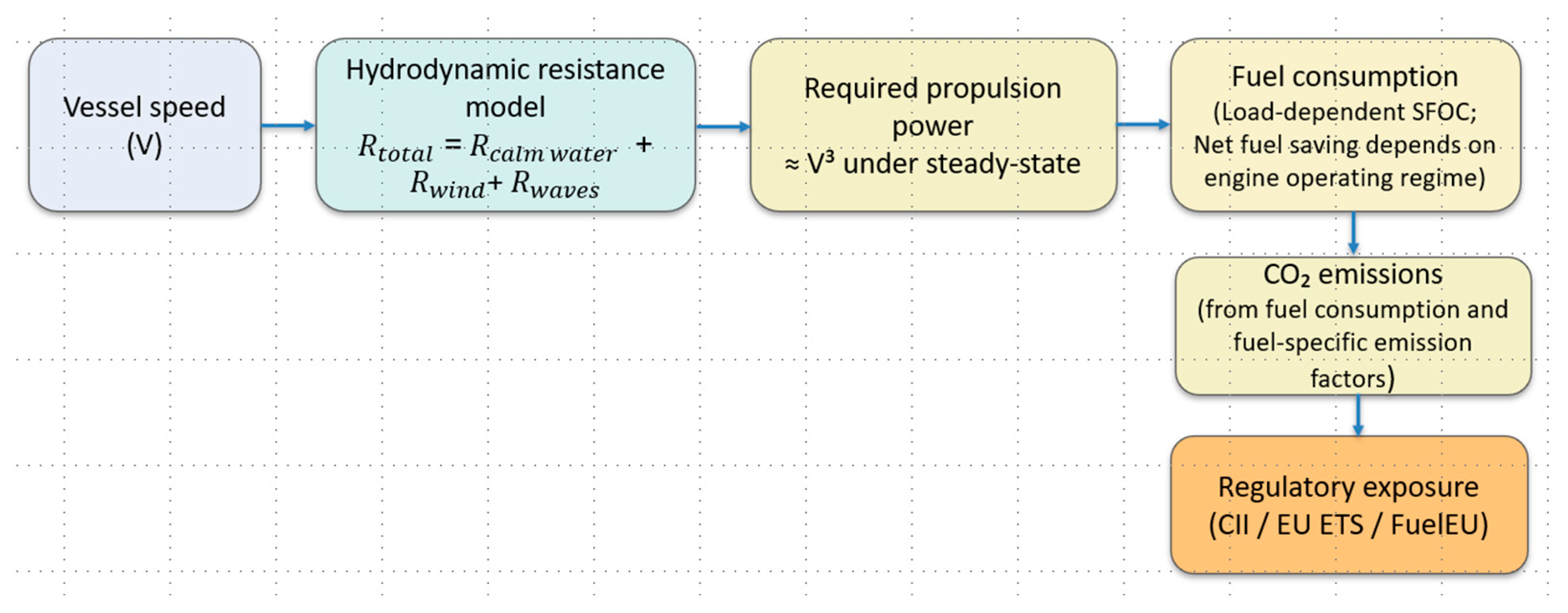
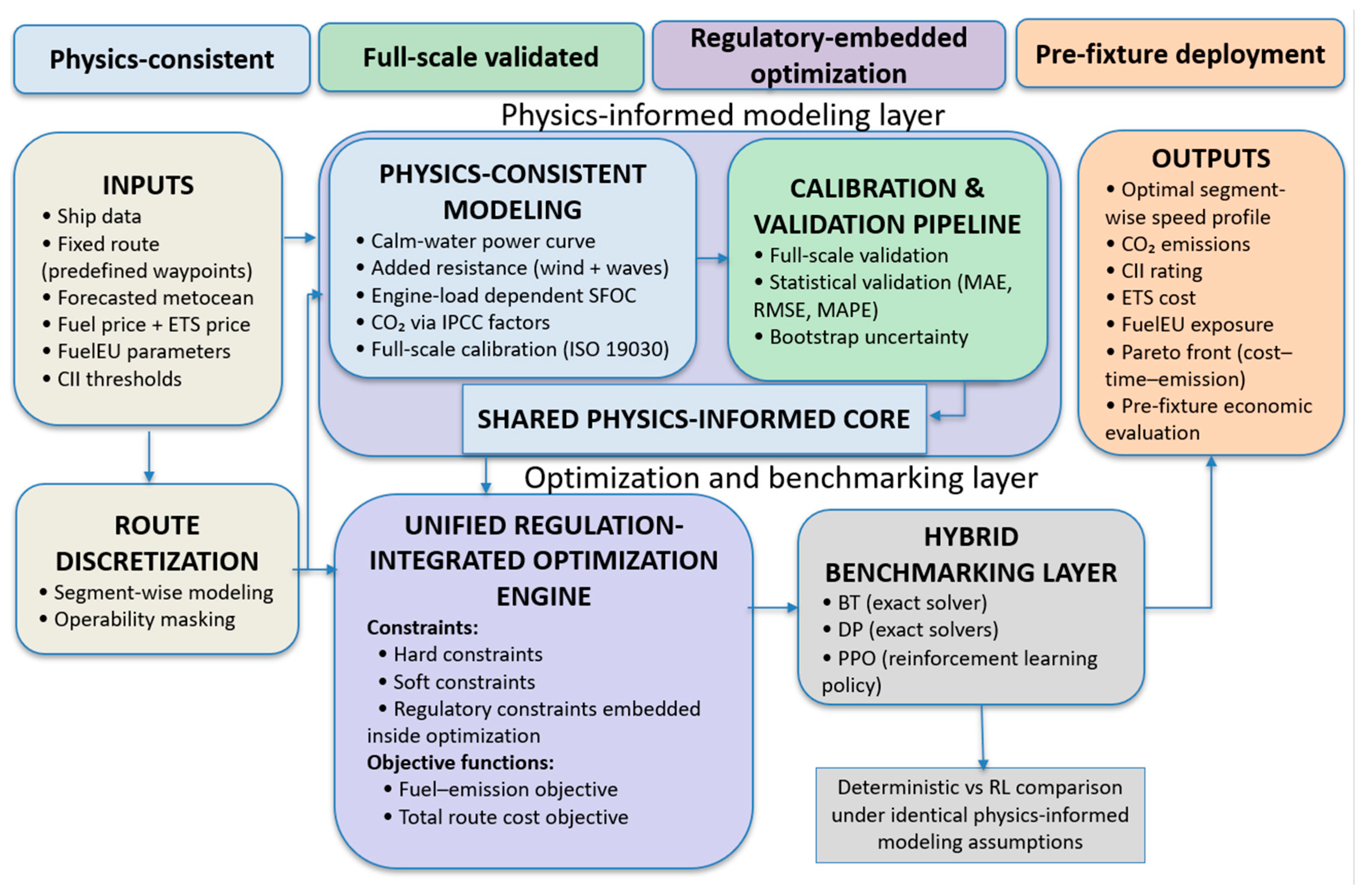
All three optimizers address the same constrained optimization problem, but differ in their computational strategy and intended role within the framework.

Backtracking and Dynamic Programming are employed as exact solvers within the discretized speed space, providing globally optimal solutions and serving as reference methods. Backtracking offers a transparent tree-based benchmark, while Dynamic Programming enables scalable exact optimization on a structured time lattice.

Proximal Policy Optimization is introduced as a learning-based alternative, aimed at approximating optimal speed-selection policies through repeated interaction with the physics-based voyage simulator.

A high-level comparison of the three approaches is provided in

Table 1. Conceptual comparison between Backtracking, Dynamic Programming, and Proximal Policy Optimization (PPO).

Element	BT	DP	PPO
State representation	Segment depth	($i,t_k$) lattice	Continuous MDP state
Optimality	Exact	Exact	Approximate
Runtime at inference	High	Medium	Negligible
Computational scaling	Exponential	Pseudo-polynomial	Training-dependent
Scalability (long routes/scenarios)	Limited	Moderate	High
Role	Gold standard	Scalable exact solver	Adaptive policy learner
Output	Optimal profile	Optimal profile	Learned speed policy

.

Exact combinatorial optimization methods have been widely used in discretized maritime speed and energy management problems, particularly for benchmarking and validation purposes [11,25,30]. Reinforcement-learning-based approaches have recently gained attention as scalable approximations for speed and power optimization under uncertainty [28].

3.4.1. Backtracking (Depth-First Search with Pruning)

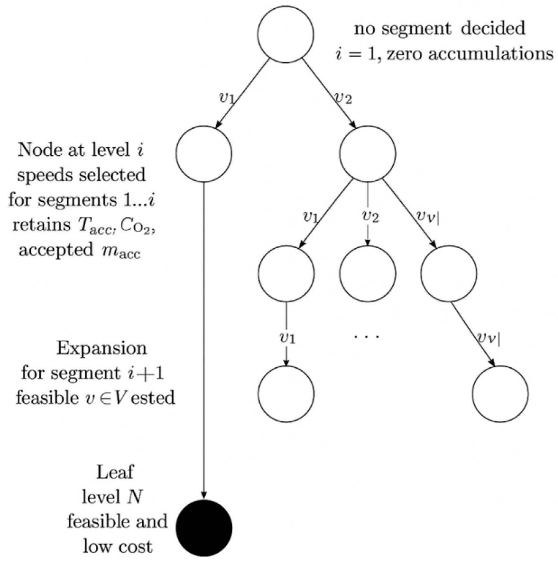
Backtracking is employed as an exact optimization method over the discrete speed space ${\mathcal{V}}^{\mathcal{N}}$ defined in Section 3.3.6. The algorithm performs a depth-first search on a segment-wise decision tree, in which each level corresponds to one route segment and each branch represents the selection of a candidate speed: $v_i\in \mathcal{V}.$

(a)

Principle

Unlike heuristic routing methods, Backtracking explicitly explores all feasible speed combinations unless eliminated by admissible pruning rules. It therefore provides a globally optimal solution within the discretized speed space and serves as a transparent reference solver against which the Dynamic Programming and reinforcement learning approaches are benchmarked.

Decision-tree formulations of this type are classical in discretized maritime speed optimization, ship energy management, and voyage planning problems, particularly when the objective function exhibits additive structure and monotonic cost accumulation [3,25,30].

(b)

Decision Structure and State Representation

The decision tree has depth $N$, corresponding to the number of route segments. At level $i$, the partial solution is defined by the fixed speed sequence: $(v_1,\dots ,v_i$).

For any such partial profile, the unified physics-informed model introduced in Section 3.2 and Section 3.3 is applied to evaluate the corresponding partial route quantities:

• Partial travel time: $T^{\left(i\right)}={\sum }_{k=1}^i{t}_k\left(v_k\right)$;
• Partial accumulated CO₂ emissions: $M_{\mathrm{C}{\mathrm{O}}_2}^{\left(i\right)}={\sum }_{k=1}^i{m}_{\mathrm{C}{\mathrm{O}}_2,k}\left(v_k\right)$;
• Partial economic and regulatory cost: $J^{\left(i\right)}={\sum }_{k=1}^i{C}_k\left(v_k\right).$

From these quantities, a partial diagnostic CII value can be computed consistently with Equation (17).

The root node (level 0 corresponds to an empty profile with zero accumulated time, emissions, and cost. A leaf node (level $N$) represents a complete feasible speed profile:

$$v=\left(v_1,\dots ,v_N\right),$$

for which $T_{route}, {\mathit{CII}}_{\mathit{route}}$ and $J_{\mathrm{route}}$ are evaluated according to Section 3.3.6.

At each expansion step, a candidate speed $v_{i+1}\in \mathcal{V}$ and the corresponding incremental physical and economic quantities are computed. The partial solution is retained only if all hard constraints defined in Section 3.3.5 are satisfied.

Decision-tree formulations of this type are classical for discretized maritime speed optimization problems [25,30]. The corresponding structure is illustrated in Figure 3.

(c)

Constraint Enforcement and Admissible Pruning

All feasibility constraints introduced in Section 3.3.5 are enforced explicitly during node expansion:

• ETA feasibility;
• Installed propulsion power limit;
• CII/CO₂ cap (when activated);
• Metocean operability constraints.

In addition, Backtracking employs admissible pruning rules that preserve global optimality while significantly reducing the explored search space:

(d)

ETA Lower-Bound Pruning

An optimistic lower bound on the remaining travel time $t_{lb}\left(i\right)$ (Equation (27)) is computed. If

$$T^{\left(i\right)}+t_{lb}\left(i+1\right)>T_{max},$$

the branch is discarded.

(e)

Emission/CII Pruning

When a regulatory cap is enforced, any partial solution for which the implied route-level CII cannot satisfy (Equation (30)) is terminated:

$$\mathrm{CI}{\mathrm{I}}_{\mathrm{route}}\le \mathrm{CI}{\mathrm{I}}_{\mathrm{allow}}.$$

(f)

Power and Operability Pruning

Candidate speeds violating the installed power limit (Equation (29)) or the metocean operability filters are discarded locally and not expanded.

(g)

Cost-based Branch-and-Bound

Since all incremental cost components defined in Equations (19)–(24) are non-negative, any partial solution satisfying the following:

$$J^{\left(i\right)}\ge J_{\mathrm{best}}$$

cannot lead to a better solution and is pruned.

All pruning rules are admissible and therefore do not exclude any globally optimal solution.

(h)

Optimality and Computational Properties

Because all feasible combinations in ${\mathcal{V}}^{\mathcal{N}}$ are explored unless eliminated by admissible bounds, Backtracking yields the global optimum of the discretized problem defined in Section 3.3.6.

Without pruning, the computational complexity is $\mathcal{O}\left({\left|\mathcal{V}\right|}^N\right).$ In practice, the combined effect of ETA, emission, power, metocean, and cost pruning reduces the explored tree by several orders of magnitude. For short- and medium-length routes, the method remains computationally efficient and provides a reliable exact benchmark for validation and sensitivity analysis [11,28].

(i)

Role within the Proposed Framework

Within the proposed hybrid framework, Backtracking fulfils three complementary roles:

(i)

Exact reference solver for the unified optimization problem;

(ii)

Validation benchmark for Dynamic Programming discretization and PPO learning outcomes;

(iii)

Transparent audit tool, providing full per-segment traceability of speed, power, fuel, emissions, and cost, consistent with ISO 19030 and ITTC recommended practices.

3.4.2. Dynamic Programming (DP) on the Time Axis for the Discretized Speed Profile

Dynamic Programming (DP) is employed as an exact optimization method formulated on a discretized cumulative-time axis. In contrast to Backtracking, which explores the combinatorial decision tree explicitly, DP propagates optimal partial solutions over a structured lattice of states indexed by segment and cumulative time.

Under the same speed discretization $\Delta V$ (Section 3.1) and a chosen time-grid resolution $\Delta t$, DP guarantees global optimality within the adopted discretization, while operating under the identical physics-informed mapping (Section 3.2 and Section 3.3) and the same hard/soft constraint logic (Section 3.3.5).

DP formulations of this type are widely used for discrete-control maritime speed optimization and routing under time and emission constraints [25,28].

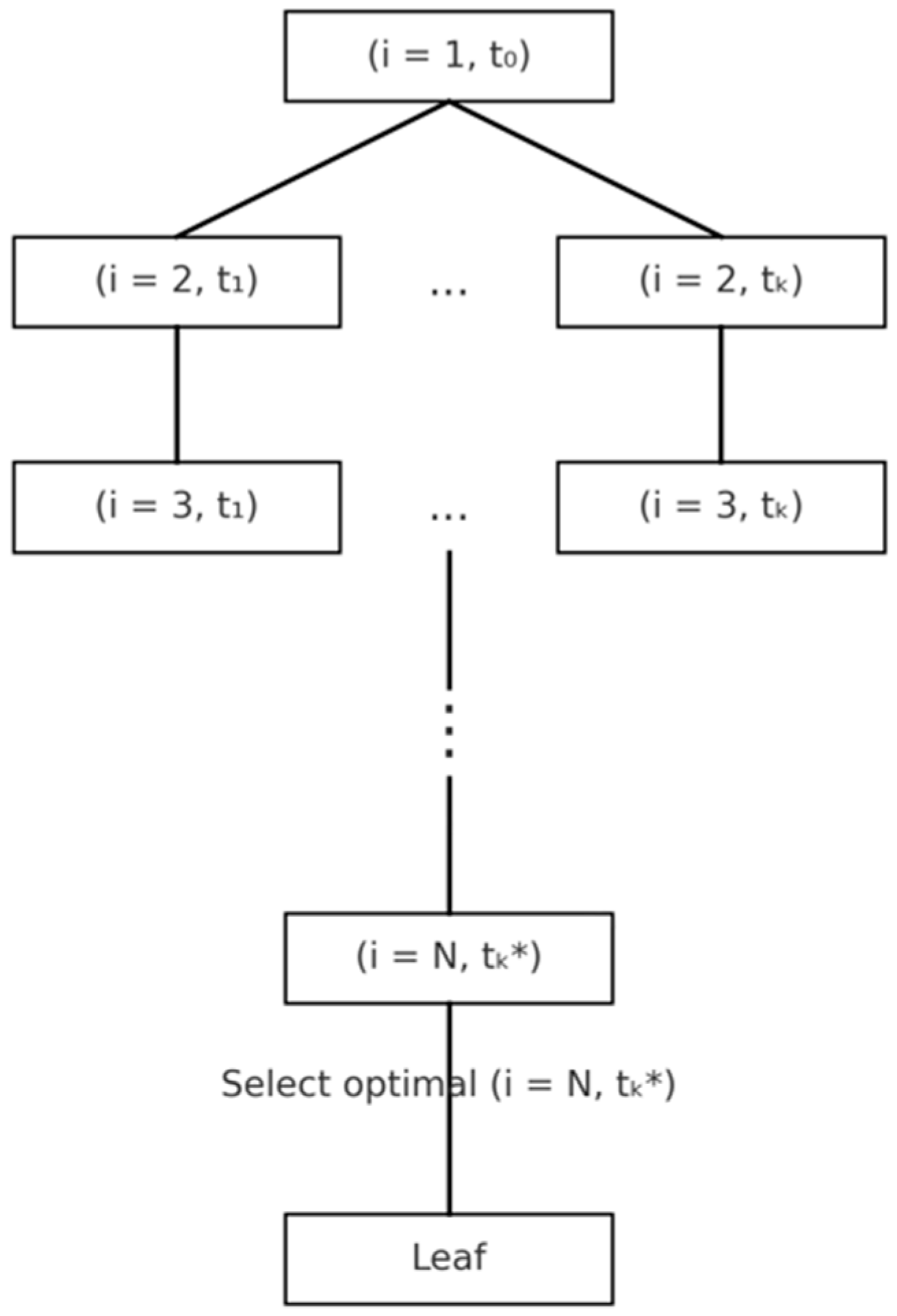
Figure 4 illustrates the lattice-based propagation of optimal partial solutions and the parent-pointer reconstruction mechanism.

(a)

Principle

DP relies on the principle of optimality: an optimal speed profile on the full route is composed of optimal partial profiles on its prefixes.

For each segment index and each admissible cumulative-time bucket, DP computes the minimum accumulated cost consistent with the selected objective $J\left(v\right)$ (Equations (25) and (26)), while enforcing all hard constraints (Equations (28)–(30)).

Soft constraints do not restrict feasibility; instead, they enter exclusively through incremental costs $C_i\left(v_i\right)$ including ETA penalties (Equations (23) and (24)) and FuelEU penalties, Equation (22).

(b)

State Space Definition

Let $\Delta t$ denote the adopted time discretization step.

The DP lattice is defined on states: $\left(i,k\right),$ where $i\in \{0,\dots ,N\}$ is the segment index and $k$ is the index of the cumulative-time bucket $t_k=k\Delta t$.

The DP value table stores the minimum accumulated cost required to reach the end of segment $i$ at cumulative-time bucket $t_k$:

$$J\left(i,k\right)= \mathrm{minimum} \mathrm{accumulated} \mathrm{route} \cos \mathrm{t} \mathrm{up} \mathrm{to} \mathrm{segment} i \mathrm{with} T\left(i\right)\approx t_k..$$

(31)

Initialization$:J\left(\mathrm{0,0}\right)=0$ and $J\left(0,k\right)=+\infty$ for $k>0.$

When a hard CII/CO₂ cap is activated, an auxiliary cumulative-emission register consistent with Equations (12)–(18), tracking cumulative CO₂ emissions up to segment $i$, may be maintained for feasibility screening, without altering the emissions model.

(c)

Transition Mechanism

From any reachable state $\left(i,k\right)$, DP evaluates all candidate speeds $v\in \mathcal{V}$ for segment $i+1$.

For each $v$, the unified physics-informed model of Section 3.2 and Section 3.3 provides:

• $\mathrm{S}\mathrm{e}\mathrm{g}\mathrm{m}\mathrm{e}\mathrm{n}\mathrm{t}\mathrm{d}\mathrm{u}\mathrm{r}\mathrm{a}\mathrm{t}\mathrm{i}\mathrm{o}\mathrm{n} t_{i+1}\left(v\right)$ (Equations (1) and (2));
• Incremental cost $C_{i+1}\left(v\right)$ consistent with Equations (19)–(24).

The continuous-time update is as follows:

$$T^{\prime }=t_k+t_{i+1}\left(v\right).$$

This value is projected onto the discretized time grid:

$$k^{\prime }=round\left({\displaystyle \frac{T^{\prime }}{\Delta t}}\right),t_{k^{\prime }}=k^{\prime }\hspace{0.17em}\Delta t$$

(32)

(d)

Constraint Enforcement (Consistent with Section 3.3.5)

A transition $\left(i,k\right)\to \left(i+1,k^{\prime }\right)$ is accepted only if all hard constraints are satisfied.

• Hard ETA feasibility:

Using the same lower-bound estimate $t_{lb}\left(\cdot \right)$ (Equation (27)):

$$t_k+t_{i+1}\left(v\right)+t_{\mathrm{lb}}\left(i+2\right)>T_{max}$$

(33)

This is equivalent in meaning to Equation (28), applied at the transition level.

• Installed power limit:

$P_{\mathrm{tot},i+1}\left(v\right)\le P_{max},$ (Equation (29)).

• Hard CII/CO2 cap (Optional):

Transitions are retained only if the cumulative emissions remain compatible with Equation (30), evaluated consistently with Equation (12)–(18).

• Metocean operability:

Metocean restrictions are enforced during preprocessing (Section 3.3.5). DP does not propagate through excluded segments or infeasible speeds.

All soft constraints enter exclusively through $C_i\left(v_i\right),$ and therefore influence the objective but not the feasibility.

(e)

Bellman Recursion

For each feasible transition, DP applies the Bellman update:

$$J\left(i+1,k^{\prime }\right)=\underset{v\in \mathcal{V}}{\min }\left\{J\left(i,k\right)+C_{i+1}\left(v\right)\right\} [€]$$

(34)

This recursion guarantees optimal substructure and preserves global optimality under discretization.

(f)

Terminal Selection and Reconstruction

At the final segment $i=N$, the algorithm inspects all admissible time buckets satisfying $t_k\le T_{max}$ and selects:

$$k^{*}=\arg \underset{k}{\min }J\left(N,k\right),$$

This defines the optimal terminal state $\left(N,t_{k^{*}}\right).$

The optimal speed profile is reconstructed through backward traversal of parent pointers:

$$\left(N,t_{k^{*}}\right)\hspace{0.25em}\to \hspace{0.25em}\left(N-1,t_{k_{N-1}}\right)\hspace{0.25em}\to \hspace{0.25em}\dots \hspace{0.25em}\to \hspace{0.25em}\left(1,t_{k_1}\right)\hspace{0.25em}\to \hspace{0.25em}\left(\mathrm{0,0}\right)$$

(35)

The propagation and reconstruction logic are shown in Figure 4.

(g)

Computational Properties

DP has pseudo-polynomial complexity driven by the number of segments N and the time-grid resolution $\Delta t$. Compared to Backtracking’s exponential scaling in ${\left|\mathcal{V}\right|}^N.$ DP trades exact combinatorial enumeration for structured lattice propagation.

This makes DP significantly more scalable for long routes or finer speed discretizations while preserving global optimality within the adopted discretization [25,28].

(h)

Role Within the Framework

Within the hybrid framework, DP serves three complementary purposes:

• Scalable exact solver with structured state propagation,
• Strong exact benchmark for PPO under identical physical and regulatory assumptions [25,28],
• Traceable optimizer, enabling full reconstruction of the optimal speed profile and segment-level accounting consistent with Section 3.2 and Section 3.3.

3.4.3. Proximal Policy Optimization (PPO) for Segment-Wise Speed Selection

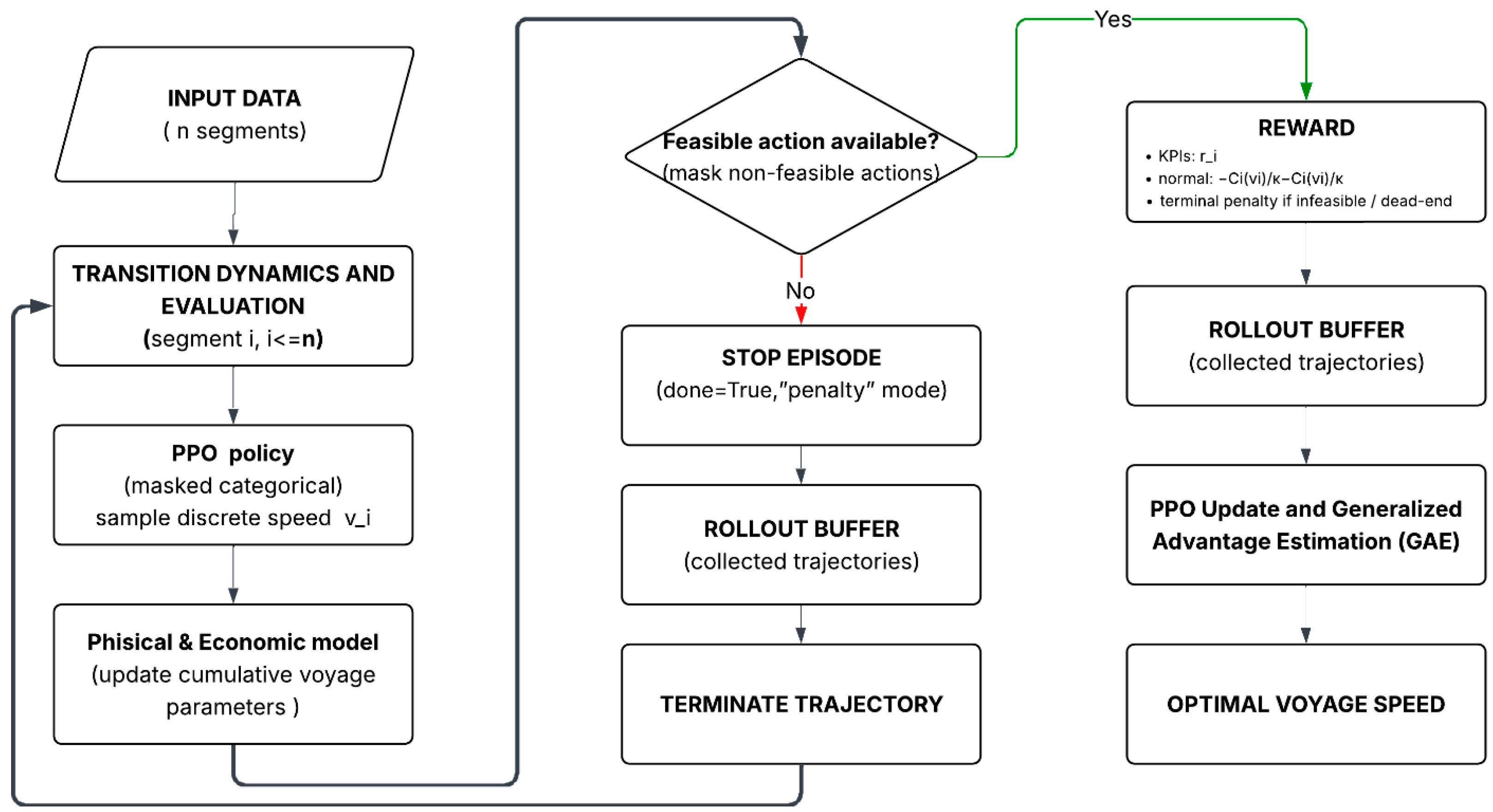
Proximal Policy Optimization (PPO) is introduced as a reinforcement learning (RL) approach for learning a segment-wise speed-selection policy within the same physics-informed environment used by the exact solvers (Backtracking and Dynamic Programming). As summarized in Table 1, PPO differs from the exact methods in that it approximates a decision rule rather than enumerating the entire discrete decision space.

Unlike heuristic RL formulations, PPO operates strictly on the unified physical, economic, and regulatory model defined in Section 3.2 and Section 3.3. No surrogate propulsion laws, simplified emission models, or alternative constraint structures are introduced. This guarantees direct comparability with Backtracking and Dynamic Programming.

Figure 5 schematically illustrates the closed-loop interaction between the PPO agent and the physics-informed route simulator, highlighting the sequential decision structure over route segments.

(a)

Reinforcement Learning Environment and MDP Formulation

The fixed-route speed optimization problem is formulated as a finite-horizon Markov Decision Process (MDP) [45], where each episode corresponds to the traversal of a route discretized into $N$ quasi-stationary segments (Section 3.1).

State Representation

At segment i the observation vector is as follows:

$$s_i= \left[d_i,c_i^{long},u_i^{wind},{\beta }_{i,rel}^{wind},H_i^{wave},{Bft}_i\right]$$

(36)

These variables correspond exactly to the segment descriptors defined in Section 3.1.

The simulator internally maintains cumulative quantities (elapsed time, fuel consumption, CO₂ emissions, CII, and total cost) computed using Equations (1)–(26). These quantities are not redefined for PPO and ensure consistency with the deterministic solvers.

(b)

Action Space and Transition Dynamics

The action corresponds to the through-water speed on segment $i$:

$$a_i=v_i\in \mathcal{V},$$

where $\mathcal{V}$ is the same discrete speed set used by Backtracking and Dynamic Programming (Section 3.1).

After selecting $v_i$, the environment transitions to state $s_{i+1}$ and all physical and economic quantities are computed using the unified mapping defined in Section 3.2 and Section 3.3:

• Propulsion power (Equation (4));
• Fuel consumption (Equations (7)–(11));
• CO₂ emissions (Equations (12)–(15));
• Incremental cost (Equations (19)–(24)).

No alternative transition model is introduced for PPO.

(c)

Constraint Handling (Consistency Section 3.3.5)

To ensure fairness in benchmarking, all hard constraints are enforced via action masking, using identical feasibility logic to that employed as pruning rules in Backtracking and Dynamic Programming:

• ETA feasibility (Equation (28));
• Installed propulsion power limit (Equation (29));
• Optional CII/CO₂ cap (Equation (30));
• Metocean operability constraints.

Infeasible speeds are removed from the admissible action set before sampling.

Soft constraints (ETA penalties and FuelEU penalties) are incorporated exclusively through the incremental cost $C_i\left(v_i\right)$ and therefore affect the reward but not the feasibility.

This unified constraint enforcement guarantees methodological consistency across all optimization methods.

(d)

Reward Design and Objective Alignment

To align PPO with the deterministic objective functions (Equations (25) and (26)), the per-step reward is defined as follows:

$$r_i=-{\displaystyle \frac{C_i\left(v_i\right)}{\mathsf{\kappa }}} [€]$$

(37)

where $C_i\left(v_i\right)$ is the incremental cost consistent with Equations (19)–(24), including any allocated route-level penalties, and κ is a scaling constant (e.g., ${10}^3),$ introduced for numerical stability.

Under feasibility-based action masking, the reward remains well shaped and does not require artificial penalty terms.

(e)

PPO Objective and Learning Mechanism

The PPO learning rule follows the canonical actor–critic structure, in which the policy is updated using a clipped surrogate objective while a separate value function estimates the expected return.

The PPO algorithm follows the clipped surrogate objective proposed by Schulman et al. [13]. The clipped objective is as follows:

$${\mathcal{L}}^{\mathrm{clip}}\left(\mathsf{\theta }\right)=\underset{\mathsf{\theta }}{\max }{\mathbb{E}}_t\left[\min \left(r_t\left(\mathsf{\theta }\right)\widehat{A_t},clip\left(r_t\left(\mathsf{\theta }\right),1-\mathsf{ϵ},1+\mathsf{ϵ}\right)\widehat{A_t}\right)\right]\hspace{0.25em}$$

(38)

with probability ratio:

$$r_t\left(\mathsf{\theta }\right)={\displaystyle \frac{{\mathsf{\pi }}_{\mathsf{\theta }}\left(a_t\right|s_t)}{{\mathsf{\pi }}_{{\mathsf{\theta }}_{\mathrm{old}}}\left(a_t\right|s_t)}}$$

(39)

The full actor–critic loss includes a value-function regression and regularization:

$$\mathcal{L}\left(\mathsf{\theta }\right)={\mathcal{L}}^{\mathrm{clip}}\left(\mathsf{\theta }\right)-{\mathsf{\beta }}_{\mathrm{ent}}\cdot \mathbb{E}\left[H\left({\mathsf{\pi }}_{\mathsf{\theta }}\left(\cdot \right|s)\right)\right]+{\mathsf{\beta }}_V\cdot \mathbb{E}\left[{\left(V_{\mathsf{\theta }}\left(s\right)-\widehat{V}\right)}^2\right]$$

(40)

Advantages are estimated using Generalized Advantage Estimation (GAE) [47]:

$$\widehat{A_t}={\sum }_{l=0}{\left(\mathsf{\gamma }\mathsf{\lambda }\right)}^l{\mathsf{\delta }}_{t+l}{\mathsf{\delta }}_t=r_t+\mathsf{\gamma }V\left(s_{t+1}\right)-V\left(s_t\right)$$

(41)

The discount factor $\gamma \in (0, 1]$ (e.g., 0.99) and $\lambda \in [0, 1]$ (e.g., 0.95), reduce variance while preserving stability.

The implementation follows the Stable-Baselines3 library [54], ensuring transparent and reproducible training.

(f)

Policy Approximation and Network Architecture

Both the policy ${\mathsf{\pi }}_{\mathsf{\theta }}$ and value function $V_{\mathsf{\theta }}$ are implemented as multilayer perceptrons with normalized inputs and categorical output over $\mathcal{V}$. Network architectures and hyperparameters are reported in Supplementary Files—File S6, while implementation details are documented in Supplementary Files—File S3.

(g)

Training Setup and Reproducibility Protocol

The PPO agent was implemented using the Stable-Baselines3 framework [54] and trained within the same deterministic, physics-informed simulation environment employed by the exact solvers. No surrogate models or simplified transition dynamics were introduced.

All training hyperparameters are explicitly reported in Supplementary Files—File S6, including learning rate, discount factor (γ), GAE parameter (λ), clipping parameter (ε), rollout length (n_steps), batch size, number of optimization epochs, entropy coefficient, total training timesteps, and network configuration. The default Stable-Baselines3 MLP actor–critic architecture was used.

A fixed random seed was adopted to ensure reproducibility of both training and policy evaluation. No route-specific hyperparameter tuning was performed. All PPO training experiments were conducted using the same deterministic simulator configuration and fixed random seed, ensuring full reproducibility of the reported optimization results.

The environment dynamics are fully deterministic, and infeasible actions are removed through strict feasibility-based action masking. Under these conditions, the PPO training process exhibits stable convergence behavior for the reported configuration.

The performance indicators presented in Section 6 correspond to the fixed training configuration defined in Supplementary Files—File S6 (including the reported hyperparameters and fixed random seed) and are directly comparable with the deterministic solutions obtained via Backtracking and Dynamic Programming.

This setup establishes a transparent and reproducible benchmarking framework for evaluating the learning-based optimizer within the proposed hybrid methodology.

(h)

Evaluation and Role within the Hybrid Framework

Backtracking and Dynamic Programming provide globally optimal solutions within the discretized decision space and serve as deterministic reference benchmarks.

PPO is evaluated under identical conditions:

• Speed discretization;
• Physics-informed model;
• Economic cost structure;
• Regulatory constraint logic.

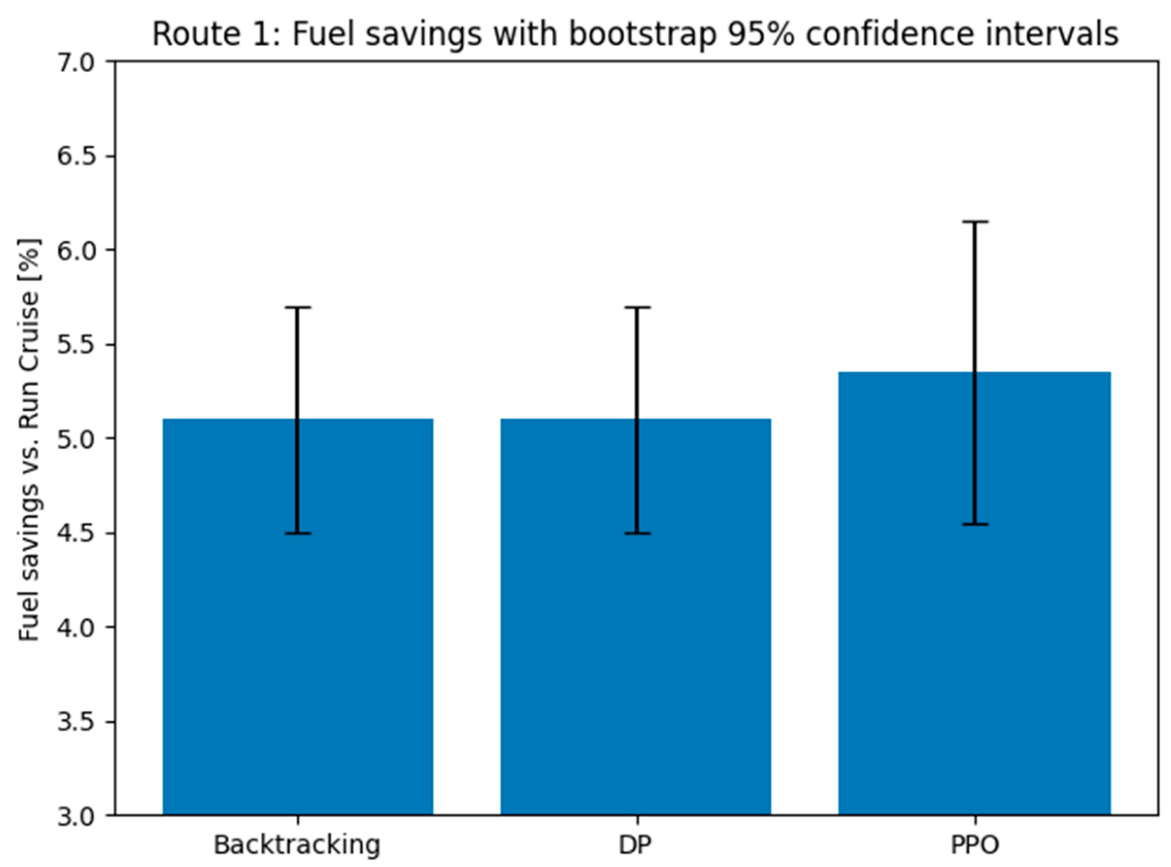
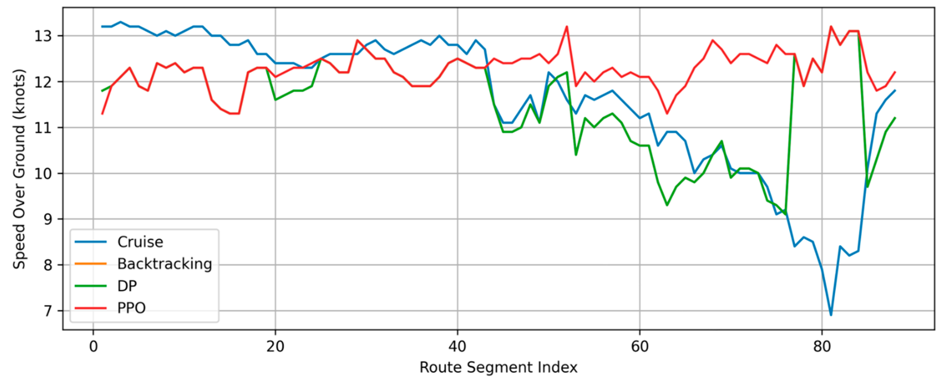
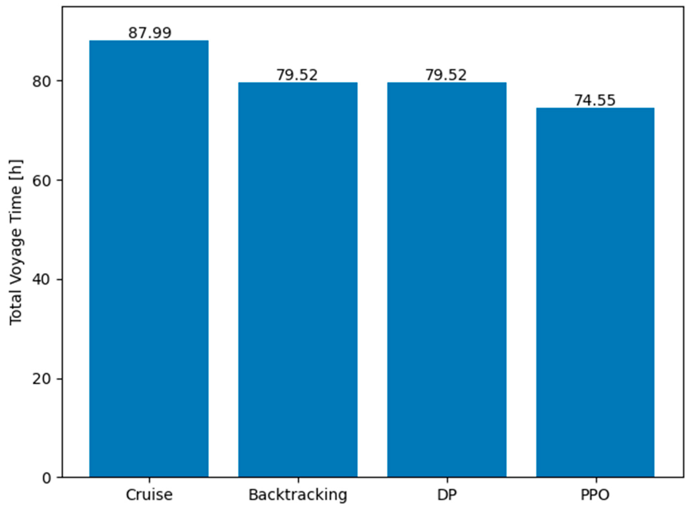
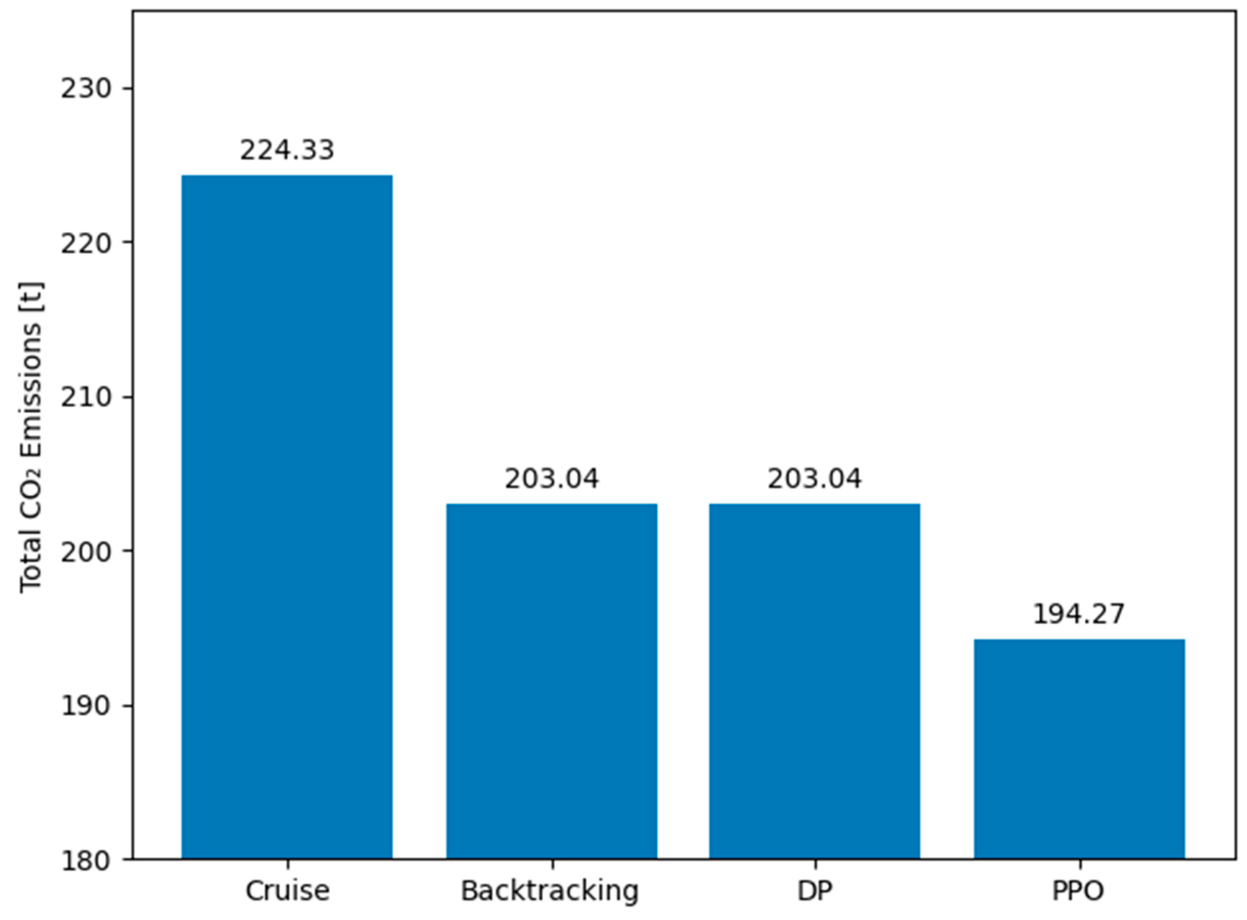
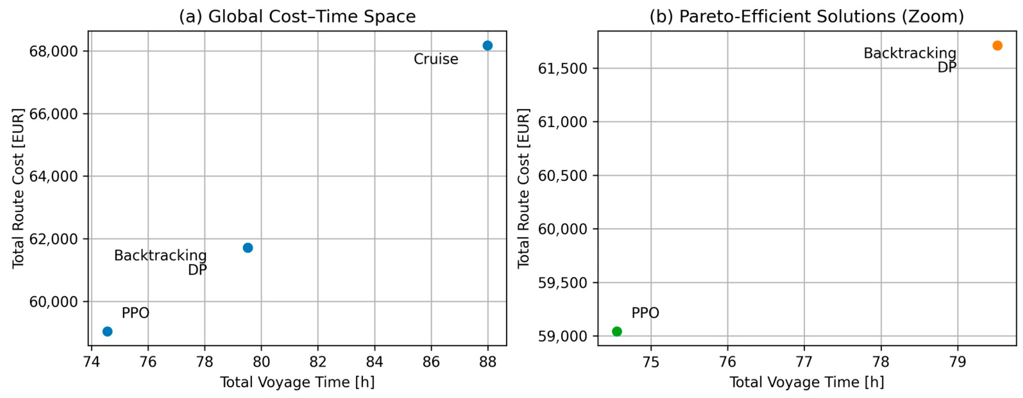
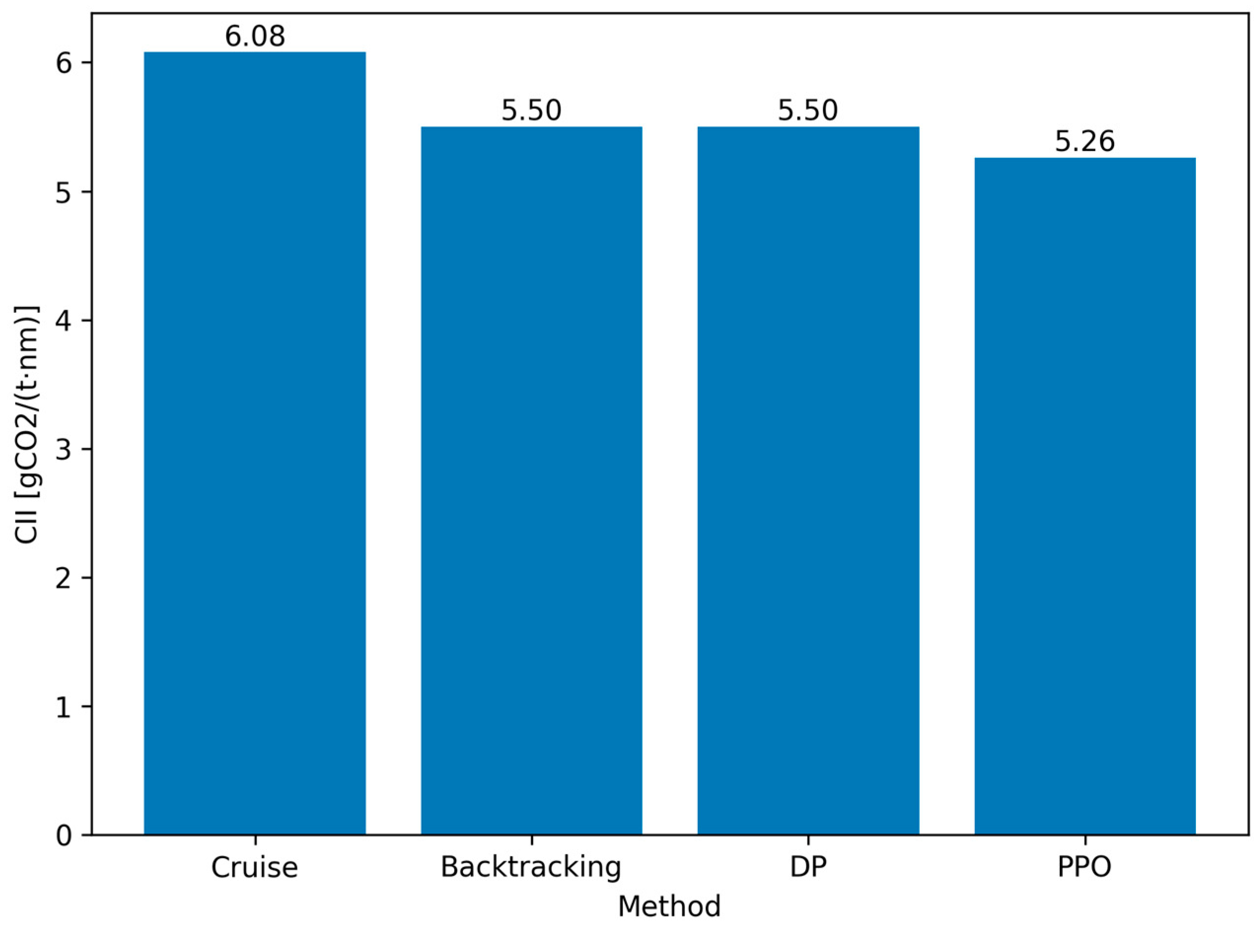
Numerical results (Section 6) show that PPO consistently produces solutions that are numerically close to the exact DP solutions in terms of fuel consumption and emissions, while often achieving shorter voyage durations through smoother segment-wise speed modulation. These results indicate empirical near-optimal performance within the discretized space, without claiming theoretical optimality.

Within the unified architecture (Figure 2 and Table 1):

• Backtracking acts as a transparent exact benchmark;
• Dynamic Programming provides scalable exact optimization;
• PPO enables scalable policy inference after offline training, allowing rapid scenario analysis under varying economic and regulatory conditions.

As summarized in Table 1, PPO differs from the exact solvers not in the underlying physical or economic model, but in the computational strategy, replacing exhaustive enumeration with learned policy approximation.

3.5. Application Validation Method

The validation of the proposed ship energy model and optimization algorithms was structured as a five-stage procedure aligned with international standards for hydrodynamic modeling, performance monitoring, and data-driven validation [19,55]. Methodological principles from numerical ship performance prediction [21], maritime data analytics, and reinforcement learning [45] were also incorporated to ensure a rigorous evaluation.

Figure 6 summarizes the logical structure of the validation workflow implemented in the Speed & Emission Optimizer application.

(a)

Stage 1—Punctual Segment Validation (Run Cruise with Real Data)

For each route, the model was executed in Run Cruise mode using measured navigational and metocean inputs for every segment: distance, SOG, current, significant wave height, wind speed and direction, and Beaufort number. The model-generated propulsion power $P_{model,i}$, segment fuel consumption, and segment travel time were computed using the Speed & Emission Optimizer and compared against ship-measured values $P_{\mathrm{real},i}$, $Fue{l}_{\mathrm{real},i} and t_{real,i}$.

In accordance with ITTC Recommended Procedures 7.5-02-07-02.2 and ISO 19030-2 [19,55] the data are statistically analyzed using the following accuracy metrics: Mean Absolute Error (MAE), Mean Squared Error (RMSE), Mean Absolute Percentage Error (MAPE), and Mean Systematic Error (Bias). The formulas for calculating these statistical metrics and the validation thresholds are presented in Supplementary Files—File S4.

This stage confirms the fidelity of the speed–power and resistance model under real operating conditions.

(b)

Stage 2—Route-Level Backtesting of Fuel Consumption

Route-level model performance was assessed using cumulative fuel consumption:

$$Fue{l}_{\mathrm{model}}=\sum _{i}Fue{l}_{\mathrm{model},i}\left[\mathrm{K}\mathrm{g}\right]$$

(42)

Relative error:

$${\mathsf{\epsilon }}_{fuel}={\displaystyle \frac{\left|Fue{l}_{model}-Fue{l}_{real}\right|}{Fue{l}_{real}}}\times 100$$

(43)

ITTC and ISO 19030 guidelines recommend acceptance levels of 8–10% for voyage-level energy predictions. This step verifies end-to-end energy estimation accuracy.

(c)

Stage 3—Cross-Route Validation via Leave-One-Route-Out (LORO)

Generalization ability was evaluated using Leave-One-Route-Out cross-validation:

• Three routes are used for calibration;
• The remaining route is used for testing.

This approach is widely used in maritime performance studies and RL evaluation frameworks [45]. For each test subset, segment-level MAE, RMSE, MAPE, and Bias were computed for propulsion power and fuel consumption. This ensures the model does not overfit a specific weather pattern or operational regime.

(d)

Stage 4—Off-Policy Validation of Optimized Speed Profiles (Backtracking, DP, PPO)

Speed profiles $V^{*}$ generated by Backtracking, Dynamic Programming, and Proximal Policy Optimization (PPO) were applied offline to the real environmental conditions of each voyage (off-policy evaluation).

Performance indicators:

$$Savin{g}_{fuel}={\displaystyle \frac{Fue{l}_{real}-Fue{l}_{model}}{Fue{l}_{real}}}\times 100$$

(44)

Additionally, CO₂ reductions, ETA compliance, and adherence to regulatory constraints (CII, ETS, FuelEU) were evaluated. This stage validates the consistency between model-based optimization and real operational behavior.

(e)

Stage 5—Robustness Assessment: Bootstrap Confidence Intervals

To quantify uncertainty, a bootstrap resampling with a sufficiently large number of iterations (at least 1000) [6] was applied to predicted fuel savings. The 95% confidence interval is computed as follows:

$${CI}_{95\%}=\left[P_{2.5\%},\hspace{0.17em}{P}_{97.5\%}\right]$$

(45)

Statistical significance of differences (e.g., DP vs. PPO, and real vs. optimized) was evaluated using paired t-tests or Wilcoxon signed-rank tests, depending on normality. This provides a rigorous, robustness assessment beyond single-sample comparisons.

(f)

Validation Strategy and Robustness Assessment

By integrating segment-level validation, route-level backtesting, cross-route generalization tests, off-policy optimization evaluation, and statistical uncertainty quantification, the proposed framework offers a comprehensive validation methodology. This exceeds the scope typically used in voyage optimization studies, reinforcing the reliability and reproducibility of the results presented.

4. Software Application for Physics-Informed Route Speed Optimization

A dedicated desktop software application, named Ship Speed & Emissions Optimizer V1, was developed to implement the proposed physics-informed hybrid framework for segment-wise route speed optimization. The application integrates the complete modeling and optimization chain introduced in Section 3, including the physical performance model, the economic and regulatory modules, and the three optimization engines (Cruise baseline, Backtracking, Dynamic Programming, and Proximal Policy Optimization). The software is designed as an applied decision-support tool, enabling direct evaluation and optimization of real fixed routes under operational, economic, and regulatory constraints. For each route segment, the application consistently computes propulsion power, fuel consumption, CO₂ emissions, CIIs, and voyage-level economic metrics, and determines feasible speed profiles that minimize either energy–emission impact or total voyage cost. A schematic overview of the software architecture is presented in Figure 7, highlighting the separation between the user interface layer and the physics-informed computational core. The complete software architecture, numerical workflow, and implementation details are provided in Supplementary Files—File S3.

4.1. Functional Scope

The Ship Speed & Emissions Optimizer supports four operational modes:

• Cruise mode, for baseline evaluation of measured voyages;
• Backtracking, providing an exact reference solution on the discretized speed space;
• Dynamic Programming, enabling scalable exact optimization on a time-discretized lattice;
• PPO mode, enabling learning-based adaptive speed optimization.

For any selected mode, the software evaluates, at the segment and route level:

• Calm-water and added environmental power;
• ME and AE fuel consumption and CO₂ emissions;
• CII, ETS exposure, and FuelEU Maritime penalties;
• ETA compliance and total voyage cost.

All calculations are based strictly on the physical and economic formulations introduced in Section 3.2 and Section 3.3, ensuring methodological consistency across deterministic and learning-based solvers.

4.2. Software Architecture and Numerical Implementation

The application follows a modular architecture composed of four tightly coupled layers: data and preprocessing, physics and performance modeling, economic and regulatory evaluation, and optimization/learning engines.

Only the functional structure and user interaction level are described in this section.

A detailed description of the following is provided in Supplementary Files—File S3 (Software architecture and numerical implementation):

• Module decomposition;
• Numerical data flow;
• Constraint-handling mechanisms;
• PPO implementation details;
• Robustness and reproducibility measures.

This separation allows the main article to focus on methodological and engineering aspects, while ensuring full technical transparency for reproducibility.

4.3. Graphical User Interface and Workflow

The graphical user interface enables full control of the optimization workflow, including the following:

• Definition and import of route segments and metocean data;
• Ship and machinery configuration;
• Regulatory and economic scenario definition;
• Solver selection and parameterization;
• Visualization and export of results.

The typical workflow consists of the following:

• Route definition and preprocessing;
• Baseline Cruise simulation;
• Exact optimization (Backtracking/DP);
• Optional PPO training and inference;
• Comparative analysis and export of results.

The implemented interface of the application is illustrated in Figure 8, which shows the main operational panels used for input definition, solver execution, and result visualization.

The detailed descriptions of each panel, including all input fields and their functions, are provided in Supplementary Files—File S3, Section S3.7.

The developed application operationalizes the proposed hybrid methodology by the following:

• Embedding a unified physics-informed performance model;
• Enforcing all hard and soft constraints defined in Section 3;
• Enabling direct benchmarking between exact optimization and PPO;
• Providing full per-segment traceability of speed, power, emissions, and cost.

By integrating physical modeling, regulatory accounting, and multiple optimization paradigms within a single computational environment, the software serves as a practical platform for both methodological validation and pre-voyage voyage decision support. From an operational perspective, it is conceived as a planning and assessment tool rather than a low-level onboard control system, enabling users to evaluate and compare candidate speed profiles under forecasted metocean and market conditions.

5. Case Study: Description and Validation Data

This section describes the real-vessel dataset and the multi-stage validation protocol used to assess both the physical fidelity of the model and the operational consistency of the optimization methods.

For the testing and validation of the proposed hybrid method, real operational data from four routes of an oil/chemical tanker were utilized.

5.1. Vessel and Route Description

The vessel characteristics obtained from onboard measurements are summarized in

Table 2. Ship Characteristics.

Characteristics	Data
Ship type	Oil Chemical Tanker
Year of construction	2007
Length between perpendiculars (Lpp) [m]	179.96
Breadth B [m]	32.3
Draft T [m]	11
Deadweight (DWT) [t]	40,439
Displacement [t]	50,029.65
Cargo capacity [m3]	38,000
Block coefficient (Cb)	0.801
Wind-exposed surface area [m2]	480
Maximum speed [kn]	16
Service (economic) speed [kn]	14.5/12

and

Table 3. Main Engine and Auxiliary Equipment Characteristics.

Characteristics	Data
Main propulsion engine (ME)	MAN B&W 6S50MC-C
Number of propulsion engines	1
Installed power [kW]	9580
Specific fuel oil consumption (SFOC) [g/kWh]	194
Fuel type	VLSFO/MDO
Towing Power [kW]	5780
Propulsive Efficiency (η)	0.6
Auxiliary Engine (AE)	20L/975W WÄRTSILÄ
Number of AEs onboard	3
Power (AE) [kW]	880
Specific fuel oil consumption (SFOC) [g/kWh]	205
Fuel type	VLSFO/MDO
CII target [g/(t∙nm)]	8.35

.

The case study vessel is equipped with a MAN B&W 6S50MC-C main engine, derated and low-load tuned, with an installed power of 9580 kW and a minimum SFOC of approximately 194 g/kWh around 50–60% MCR. The service speed before tuning was 14.5 kn (≈60% MCR), while the post-tuning economic speed used in the optimization scenarios is 12 kn, corresponding to approximately 35–45% MCR.

The four fixed routes used for testing and validation are presented in

Table 4. Routes.

No	Routes	Distance [NM]	Period	ETA [h]	Cargo [mt]
1.	Milazzo–Motril	920	19/03/2025–23/03/2025	90	29.918
2.	Livorno–Sarroch	278	22/06/2025–23/06/2025	25	0
3.	Messina–Fiumicino	348	20/08/2025–21/08/2025	30	30.044
4.	Bar–Sidi Kenir	880	14/09/2025–17/09/2025	80	0

.

The data from the four ship-collected routes used in the study are presented in Supplementary Files—File S5. In accordance with the recommendations of ITTC [18] and ISO 19030 [35], the segments corresponding to port entry/exit and anchorage were excluded because they do not represent normal navigation conditions. During these intervals, the main engine operates outside the P-V characteristic range, maneuvers introduce lateral components and sudden speed variations, and fuel consumption is dominated by auxiliary thrusters and generators.

5.2. Economic Parameters

The economic parameters of the ship (fuel price, ETS, FuelEU, Charter) [56] for the four routes subject to the study are presented in Supplementary Files—File S5.

5.3. Global Calibration of Hydrodynamic and Aerodynamic Components

To ensure that the model replicates the vessel’s real operational behavior with high fidelity, the input parameters used in the application must closely reflect the physical characteristics of the ship under study. The variables that exert the strongest influence on ship speed are the propulsion power, represented by the calm-water power–speed relationship $P_{\mathrm{calm}}\left(V\right)$, and the aerodynamic response described by the coefficient $C_D\left(\mathsf{\beta }\right)$. For this reason, the application allows both curves to be supplied explicitly as user-defined inputs.

All these parameters were calibrated using the full-scale measurements collected during the four routes, ensuring that the hydrodynamic, aerodynamic, and fuel-consumption characteristics incorporated in the model are grounded in real operational data rather than theoretical approximations.

5.4. Validation Workflow and Robustness

Building on the Application Validation Method introduced in Section 3.5, this section presents the practical implementation and results of the multi-stage validation framework applied to the proposed physics-informed hybrid optimization model. The objective is to demonstrate that the underlying physical model, together with the exact (Backtracking and Dynamic Programming) and learning-based (PPO) optimization approaches, is accurate, robust, and reproducible under real operational conditions, in accordance with ITTC [19] and ISO 19030 recommendations [35].

The validation strategy is structured into five consecutive stages, each addressing a distinct aspect of model fidelity, generalization, and robustness. Importantly, Backtracking and Dynamic Programming are treated as exact solvers on the discretized speed–time space and serve as deterministic benchmarks, against which the behavior and convergence of the PPO-based policy are assessed.

5.4.1. Validation Dataset and Segmentation

The validation is performed using a multi-route dataset comprising four real voyages (two cargo-loaded and two ballast trips), selected to ensure sufficient variability in ship displacement, propulsion loading, and environmental forcing. This dataset spans a wide range of wind directions, wave heights, current regimes, and engine operating conditions, enabling a statistically meaningful evaluation of both physical and algorithmic components.

Although the dataset contains four voyages of a single vessel, the segmentation into 213 quasi-stationary route segments provides a statistically meaningful validation sample covering a wide range of environmental operating conditions.

Each route is discretized into quasi-stationary segments of 10–14 nautical miles, consistent with ISO 19030 guidelines for full-scale performance analysis. Segment-wise averaging mitigates short-term stochastic effects (e.g., gusts, wave groups, and current shear), allowing stable estimation of hydrodynamic resistance, aerodynamic loading, and engine performance. This segmentation also reduces short-term temporal correlation between consecutive observations, allowing segments to be treated as approximately independent samples for statistical analysis.

For each segment, the following measured inputs are used:

• Speed through water (STW);
• Main engine (ME) power;
• ME and auxiliary engine (AE) fuel consumption;
• Wind speed and relative wind direction;
• Significant wave height $H_s$;
• Longitudinal current component;
• Cargo mass and loading condition.

This configuration defines a validation dataset that is both physically representative and sufficiently rich for rigorous statistical analysis.

5.4.2. Segment-Level Statistical Error Distribution (Stage 1)

Stage 1 of the validation methodology (see Section 3.5) requires analyzing the statistical behavior of segment-level prediction errors in order to determine whether the model exhibits structural bias, excessive dispersion, or non-physical residual patterns. This step is essential for establishing whether the residuals reflect natural metocean and measurement variability, or if they instead indicate deficiencies in the hydrodynamic, aerodynamic, or $SFOC$ components of the model.

To characterize this behavior, the normalized prediction error for ME power was computed for each segment across all routes. The resulting distribution is shown in Figure 9. The distribution aggregates N = 213 quasi-stationary route segments obtained from four real voyages, ensuring statistically meaningful inference while remaining fully consistent with the available full-scale dataset.

The histogram in Figure 9 is superimposed with a fitted Gaussian distribution. The mean of the error distribution lies very close to zero, indicating the absence of systematic bias, while the empirical standard deviation is σ ≈ 0.04718. The vertical lines indicate the mean (μ), the ±1σ interval, and the ±2σ interval, the latter enclosing approximately 95% of the observations. This behavior confirms that the model residuals exhibit near-Gaussian characteristics under real-sea operating conditions.

Interpretation and Validation (Stage 1 Requirements)

(a)

Absence of structural bias—symmetric error distribution

The lateral deviations bounding the distribution (−0.04581 and +0.04664) are nearly identical, confirming a high degree of symmetry. This implies the following:

• No systematic tendency to overpredict or underpredict ME power;
• A mean residual effectively equal to zero;
• Compliance with Stage 1 bias criteria.

This observation is consistent with the low Bias_p (%) obtained in the KPI analysis, reinforcing that the model calibration successfully removed systematic drift.

(b)

Narrow distribution width—high precision of segment-level predictions

The tight clustering around the mean (σ ≈ 0.047) indicates the following:

• Most prediction errors fall within a narrow range;
• Residual variability is dominated by environmental fluctuations and sensor noise;
• The model generalizes consistently across all routes.

The ±2σ interval captures nearly all errors, demonstrating stable and well-behaved residuals, as required in Stage 1.

(c)

Gaussian behavior—physically meaningful residuals rather than structural flaws

The strong agreement between the histogram and the fitted Gaussian curve shows the following:

• Errors arise from natural stochastic variability (wind gusts, current shear and wave groups);
• No numerical artifacts or modeling discontinuities are present;
• The calibrated model captures the primary physical drivers of propulsion power.

A near-Gaussian residual distribution is a hallmark of a correctly specified physical model and satisfies Stage 1 requirements for distribution shape and normality.

(d)

Large sample size—robustness of statistical inference

The histogram aggregates approximately $5\times {10}^5$ segment samples across the four routes.

This extensive dataset:

• Reduces statistical uncertainty;
• Supports reliable cross-validation procedures (LORO);
• Provides the necessary depth for stable estimation of $C_D\left(\beta \right)$, RAW scaling, and SFOC correction.

Thus, the dataset satisfies the Stage 1 requirement for sufficiently rich and diverse data.

Summary of Stage 1 Validation Outcome

The segment-level analysis demonstrates the following:

• The error distribution is centered, symmetric, and unbiased;
• Dispersion is low and stable across routes;
• Residuals follow a near-Gaussian pattern expected in real-sea performance data;
• The dataset is large enough to ensure statistical robustness.

Accordingly, Stage 1 of the validation process is successfully satisfied, enabling progression to Stage 2 (route-level KPI validation against ITTC and ISO thresholds).

5.4.3. Route-Level KPI Validation Against ITTC and ISO Criteria (Stage 2)

Stage 2 evaluates the accuracy of the calibrated model at the route level using standardized Key Performance Indicators (KPIs) directly comparable with the thresholds recommended by ITTC 7.5-02-07-02.2 and ISO 19030-2.

Route-integrated fuel consumption is computed using Equation (43), while the relative fuel prediction error is evaluated using Equation (44). Additional KPIs include RMSE_p, MAPE_p, Bias_p and${\mathit{\epsilon }}_{\mathit{f}\mathit{u}\mathit{e}\mathit{l}}$, normalized according to ITTC and ISO procedures.

The full set of validation metrics is summarized in

Table 5. Validation KPIs for main engine power.

Route	Seg. [N]	$\mathit{M}\mathit{A}{\mathit{E}}_{\mathit{P}} [$kW]	$\mathit{R}\mathit{M}\mathit{S}{\mathit{E}}_{\mathit{P}} [$kW]	$\mathit{R}\mathit{M}\mathit{S}{\mathit{E}}_{\mathit{P}} [$%]	$\mathit{M}\mathit{A}\mathit{P}{\mathit{E}}_{\mathit{P}} [$%]	$\mathit{B}\mathit{i}\mathit{a}{\mathit{s}}_{\mathit{P}} [$kW]	$\mathit{B}\mathit{i}\mathit{a}{\mathit{s}}_{\mathit{P}} [$%]
Milazzo–Motril	88	159.41	204.21	5.81	4.56	149.07	4.24
Livorno–Sarroch	21	234.43	236.08	7.64	7.59	234.43	7.58
Messina–Fiumicino	28	314.34	318.58	9.60	9.60	261.20	7.98
Bar–Sidi Kenir	76	168.72	258.54	5.01	5.01	63.93	1.90

and

Table 6. Validation KPIs for main fuel across four routes.

Route	Seg. [N]	MAE [t/h]	RMSE [t/h]	MAPE [%]	Bias [t/h]	Fuel Error [%]
Milazzo–Motril	88	0.0650	0.2836	5.25	0.05945	5.25
Livorno–Sarroch	21	0.11447	0.3541	4.27	0.03881	5.07
Messina–Fiumicino	28	0.02420	0.3562	3.30	–0.00986	1.42
Bar–Sidi Kenir	76	0.07534	0.31738	4.72	–0.07118	4.44

.

A comparative overview of RMSE_p and Bias_p across the four routes is presented in Figure 10, together with the ITTC tolerance bands for calm-water and moderate-wave conditions. As shown in Figure 10, all routes remain within the recommended limits, with only minor variations attributable to differences in metocean forcing and loading conditions.

Stage 2 validation outcome

Based on the formal KPI assessment:

• RMSE_p (%) < 10–12% → satisfies ITTC requirements;
• Bias_p (%) within ±5% for three routes → acceptable for moderate-wave operation;
• MAPE_p (%) < 10% → satisfies ISO 19030;
• ${\epsilon }_{fuel}$ (%) < 6% → significantly better than ISO’s 8–10% acceptance range.

These results demonstrate that segment-level prediction errors do not accumulate at voyage scale and that end-to-end energy prediction accuracy is preserved, thereby fulfilling the requirements of Stage 2 validation.

This provides the foundation for Stage 3, which evaluates inter-route consistency and generalization robustness.

5.4.4. Cross-Route Robustness (Stage 3)

Stage 3 assesses the robustness and generalization capability of the model across different routes. This evaluation is performed using two complementary approaches: cross-route distributional analysis and Leave-One-Route-Out (LORO) validation. Figure 11 illustrates the cross-route error distributions through boxplots of segment-level power prediction errors, showing HD95 (a) and mDTA (b) metrics grouped by anatomical structure (Brainstem, L Parotid, R Parotid, and S. cord), where the compact interquartile ranges and consistent median values across all routes confirm that both CNN models achieve stable and generalizable prediction accuracy independent of route-specific characteristics.

(a)

Cross-route distributional analysis

Cross-route error distributions are illustrated in Figure 11, which presents boxplots of absolute segment-level ME power prediction errors grouped by route. The compact interquartile ranges (IQRs) and similar median values observed in Figure 11 indicate that prediction accuracy is stable and largely independent of route-specific characteristics.

Outliers present in the distributions are primarily associated with segments affected by localized metocean disturbances and are consistent with ISO 19030 expectations for full-scale operational data. The absence of systematic drift across routes confirms that the calibrated physical model generalizes well across variations in displacement, environmental conditions, and propulsion loading.

(b)

Leave-One-Route-Out (LORO) generalization test

Results of LORO analysis:

• ${\mathit{\epsilon }}_{\mathit{f}\mathit{u}\mathit{e}\mathit{l}}$ (%) remained below 6% in all validation scenarios, confirming that energy prediction accuracy does not degrade when the model is applied to routes outside the training set.
• RMSE_p (%) and Bias_p (%) exhibited only minor variation between LORO and full-dataset calibration, demonstrating that the physical components of the model retain their structure under partial-data recalibration.
• The error distribution maintained a stable Gaussian-like shape, with no increase in skewness or kurtosis, further reinforcing the conclusions from Stage 1.

The LORO results confirm that the calibrated model achieves a high degree of generalization capability, enabling accurate prediction on new routes without requiring re-tuning of parameters. This aligns with the expected behavior of physically grounded hybrid methods and is essential for operational deployment in real-time optimization or regulatory compliance workflows.

The combination of cross-route distributional analysis and LORO generalization testing demonstrates the following:

• The model performance is highly stable across different operational conditions;
• Prediction quality does not depend on specific route characteristics;
• The error structure remains well behaved and unbiased;
• Integrated energy accuracy (${\epsilon }_{fuel}$) remains consistently within ISO limits;
• The model satisfies all robustness criteria defined in Stage 3.

Together with the results of Stages 1 and 2, these findings confirm that the model is fully validated, physically consistent, and operationally reliable for multi-route prediction of ME power and fuel consumption.

5.4.5. Model Comparison and Clustering-Based Validation (Stage 4)

Stage 4 of the validation methodology, as defined in Section 3.5, focuses on the comparative assessment of prediction models and on evaluating the impact of operational clustering on segment-level accuracy. This stage extends the physical-model validation performed in Stages 1–3 by benchmarking alternative regression approaches and by analyzing their robustness under different metocean and operational regimes.

The objective of Stage 4 is two-fold:

i.

To determine whether purely data-driven or hybrid machine learning (ML) models can outperform or complement the calibrated physical model;

ii.

To assess whether physically meaningful clustering of operating conditions improves prediction accuracy and stability, as hypothesized in the validation methodology.

(a)

Baseline comparison without clustering

The left panel of Figure 12 (“No clustering”) presents the distribution of segment-level fuel prediction errors, expressed through RMSE, for six commonly adopted regression models: XGBoost (XGB), AdaBoost (ADA), k-Nearest Neighbours (KNN), Random Forest Regression (RFR), Support Vector Regression (SVR), and Lasso regression.

Two complementary indicators are analyzed: the median RMSE, reflecting typical prediction accuracy, and the interquartile range (IQR), reflecting robustness and sensitivity to operational variability.

The results indicate that gradient boosting models (XGB and ADA) achieve the lowest median RMSE values and the most compact IQRs, demonstrating both high accuracy and strong stability across the four routes. KNN and RFR exhibit moderate performance, with slightly broader dispersion but acceptable robustness. In contrast, SVR and Lasso show the largest error variability and extended outlier ranges, highlighting their sensitivity to nonlinear effects and rapidly changing metocean conditions.

This baseline comparison confirms that ensemble-based nonlinear models are inherently better suited to full-scale operational data, where residual variability arises from complex interactions between wind, waves, currents, and propulsion dynamics. Individual points outside the whiskers represent outliers—data points where the prediction error significantly exceeds the typical range, likely caused by abnormal operating conditions or measurement noise in the dataset.

(b)

Clustering under low-energy operational conditions (Cluster 0)

The central panel of Figure 12 (“Cluster 0”) evaluates model performance under relatively homogeneous environmental conditions, characterized by low wind speeds, weak currents, and limited wave-height variability.

Under these conditions, all models experience a marked reduction in RMSE, confirming that environmental homogeneity naturally increases prediction stability. XGB, ADA, and KNN exhibit particularly compact IQRs, indicating high consistency and minimal sensitivity to small variations in segment characteristics. SVR and Lasso remain the most variable models, confirming that linear or heavily regularized approaches struggle even under benign conditions.

These results directly support the Stage 4 hypothesis formulated in Section 3.5, namely that operational clustering enhances prediction accuracy, especially for models capable of representing nonlinear relationships.

(c)

Clustering under high-energy metocean conditions (Cluster 1)

The right panel of Figure 12 (“Cluster 1”) focuses on segments dominated by strong metocean forcing, including wind speeds of 6–10 m/s, significant wave heights exceeding 1.5 m, and irregular current fields.

As expected, all models exhibit increased RMSE, confirming that environmental forcing is the dominant driver of prediction uncertainty in real-sea conditions. Nevertheless, XGB remains the most robust method, with a relatively low median RMSE and controlled dispersion. ADA also maintains predictable error behavior, whereas KNN and RFR show increased variability. Lasso experiences the most severe degradation, with very large dispersion and the highest RMSE values, while SVR displays pronounced sensitivity to metocean variability, reflecting kernel rigidity under rapidly changing conditions.

These findings demonstrate that only robust nonlinear ensemble models preserve acceptable accuracy in high-energy operational environments, in full agreement with the objectives of Stage 4.

(d)

Implications of clustering and model comparison (Stage 4 conclusion)

The comparative results across the three scenarios (no clustering, Cluster 0 and Cluster 1) lead to the following conclusions:

• Gradient boosting models (XGB and ADA) consistently outperform all other methods in terms of accuracy and robustness across routes and environmental regimes
• Operational clustering significantly improves prediction stability, particularly under low-energy conditions.
• In high-energy metocean states, acceptable performance is maintained only by models capable of representing nonlinear interactions.
• Linear or regularization-based models (Lasso, SVR) are inadequate for full-scale ship performance modeling under real-sea conditions.
• The observed clustering-enhanced performance directly supports the multi-stage validation framework defined in Section 3.5, demonstrating that physically meaningful segmentation improves both interpretability and predictive robustness.

Final Validation Statement for Stage 4

Stage 4 confirms that the adopted hybrid modeling framework is competitive with, and often superior to, advanced ML alternatives, that environmental clustering significantly enhances accuracy and stability, and that reliable prediction performance is maintained across both low- and high-energy operational regimes. Together with the results from Stages 1–3, these findings demonstrate that the proposed framework satisfies the comparative and robustness requirements of Stage 4 and provides a solid foundation for the final uncertainty and robustness assessment in Stage 5.

5.4.6. Global Stability, Uncertainty Assessment and Final Validation (Stage 5)

Stage 5 provides the final robustness and uncertainty assessment of the proposed speed optimization framework by quantifying the statistical significance and stability of the observed performance gains. The analysis is conducted for Route 1 (Milazzo–Motril), which is subsequently used as the detailed optimization case study in Section 6.

Bootstrap resampling with B = 2000 iterations was applied to the segment-level fuel consumption differences between real-speed Cruise operation and the optimized speed profiles obtained using Proximal Policy Optimization (PPO). Total fuel consumption was evaluated as the sum of main engine (ME) and auxiliary engine (AE) fuel consumption at the segment level. The corresponding 95% confidence interval for the route-level fuel savings was computed using Equation (45), yielding the following:

CI_95% = [4.57%,6.37%]

The strictly positive and relatively narrow confidence interval indicates that fuel savings are consistent across route segments and robust to sampling variability, providing strong statistical evidence of the effectiveness of the optimization.

Normality of the paired segment-level fuel consumption differences (Run Cruise vs. optimized profiles) was assessed using the Shapiro–Wilk test, which indicated non-normality of the distribution. Consequently, the Wilcoxon signed-rank test was applied, confirming that the fuel savings relative to Cruise operation are statistically significant ($p=9.54\times {10}^{-7}$).

The resulting bootstrap confidence intervals, illustrated in Figure 13, are narrow and non-overlapping with zero, further supporting the robustness and statistical reliability of the observed optimization gains at the route level. Quantitatively, the mean route-level fuel savings relative to real-speed Cruise operation amount to approximately 5.11% for both Backtracking and Dynamic Programming, with identical 95% confidence intervals of [4.45%, 6.09%]. The PPO-based solution achieves a slightly higher mean fuel saving of 5.35%, with a 95% confidence interval of [4.56%, 6.38%], while preserving statistical robustness.

Bars indicate the mean route-level fuel savings obtained using Backtracking, Dynamic Programming (DP), and Proximal Policy Optimization (PPO), computed from segment-level data. Error bars represent the 95% confidence intervals estimated via bootstrap resampling (B = 2000). All intervals are strictly positive, confirming statistically significant and robust fuel savings across route segments.

By integrating segment-level validation, route-level backtesting, off-policy optimization evaluation, and statistical uncertainty quantification, Stage 5 confirms that the proposed framework is robust, reproducible, and suitable for operational deployment and regulatory assessment. The consistency between the statistical validation results presented here and the deterministic optimization outcomes analyzed in Section 6 provides a strong foundation for the practical applicability of the proposed decision-support framework.

Consistency Statement (Methodology–Results Alignment)

Each validation stage presented in this section directly corresponds to the stages defined in Section 3.5, employing consistent metrics, acceptance criteria, and statistical procedures. This ensures full methodological coherence between the validation design and its practical implementation.

6. Case Study: Route Speed Optimization Under Economic and Regulatory Constraints

6.1. Route Description and Case Study Objectives

This case study analyzes the practical behavior and decision-making characteristics of three segment-wise speed optimization approaches—Backtracking, Dynamic Programming (DP), and Proximal Policy Optimization (PPO)—when applied to a fixed maritime route under identical physical, economic, and regulatory conditions.

The analyzed voyage corresponds to Route 1 (Milazzo–Motril), discretized into 88 sequential segments, and evaluated using the fuel-emission objective, which prioritizes the minimization of total fuel consumption and CO₂ emissions while preserving ETA feasibility. The objective of this section is not limited to a numerical comparison of route-level outputs, but rather to examine how each optimization paradigm exploits segment-wise speed selection and how this translates into differences in voyage time, fuel consumption, CO₂ emissions, total route cost, and compliance with the Carbon Intensity Indicator (CII).

Real-speed Cruise operation is considered exclusively as a baseline reference. The analytical focus of this section is placed on the comparative performance of the three adaptive optimization methods.

This ensures that the results discussed in Section 6.3, Section 6.4, Section 6.5, Section 6.6, Section 6.7 and Section 6.8 reflect algorithmic differences rather than modeling artifacts.

6.2. Route Definition and Input Consistency

The analyzed route is discretized into sequential segments, each annotated with distance, longitudinal current, wind conditions, significant wave height, and Beaufort number, following the methodology introduced in Section 3.1.

To ensure a fair and transparent comparison, all optimization methods operate under strictly identical input conditions, including the following:

• The same route geometry and segmentation (88 segments);
• Identical metocean and navigational inputs at the segment level;
• A shared physics-informed model for propulsion power, fuel consumption, and CO₂ emissions;
• Identical regulatory parameters, including EU ETS pricing and the vessel-specific CII target.

This strict input consistency guarantees that any observed differences in performance arise solely from the optimization logic rather than from modeling or parameterization artifacts.

6.3. Optimized Speed Profiles and Voyage Time Comparison

This section demonstrates how different optimization paradigms exploit segment-wise speed variability to achieve distinct voyage-time outcomes under identical constraints.

Figure 14 illustrates the segment-wise speed-over-ground (SOG) profiles obtained for the Milazzo–Motril route under real-speed Cruise operation and the three adaptive optimization methods. The Cruise profile reflects the recorded operational speeds along the route and serves as a reference for assessing the effect of optimization.

Backtracking and Dynamic Programming converge to the same globally optimal solution within the adopted discretized formulation. As a result, their SOG profiles are numerically identical and fully overlap in Figure 14. This confirms the consistency of the exact discrete optimization framework.

The PPO-based approach produces a distinct adaptive profile, reflecting its policy-learning mechanism under the same physics-informed model and constraint structure. Despite methodological differences, all adaptive solutions deviate significantly from the Cruise baseline, demonstrating the operational impact of segment-wise speed optimization.

Although all adaptive methods respect identical physical and regulatory constraints, the resulting speed profiles differ in smoothness and aggressiveness, which provides the voyage-time differences reported in Figure 15.

The Cruise speed profile exhibits limited adaptation to local environmental conditions, resulting in relatively uniform speed patterns across consecutive segments. In contrast, all adaptive optimization methods introduce deliberate speed modulation, adjusting segment-wise SOG in response to spatial variations in resistance, currents, and metocean conditions.

Backtracking and Dynamic Programming produce closely aligned speed profiles, confirming that both exact optimization methods converge toward similar segment-level decisions when operating under identical physical and regulatory constraints. These profiles exhibit discrete speed adjustments, reflecting the underlying discretization of the decision space.

The PPO-based solution displays a smoother speed profile, characterized by gradual transitions between adjacent segments. Despite this smoother modulation, PPO achieves comparable or superior performance in terms of voyage duration and energy efficiency. This indicates that reinforcement learning is able to internalize the physics-informed cost structure and regulatory constraints, generating coherent speed policies without explicit enumeration of the speed–time search space.

The impact of speed modulation on overall voyage duration is summarized in Figure 15 which compares the total voyage time obtained for each method.

Cruise operation results in the longest voyage duration (87.99 h), while all adaptive optimization strategies achieve substantial time reductions. Backtracking and DP reduce the voyage time to 79.52 h, corresponding to a reduction of approximately 9.6% relative to Cruise. PPO achieves the shortest voyage duration (74.55 h), representing a total reduction of approximately 15.3%.

The shorter voyage time obtained by PPO does not result from constraint relaxation, but from a learned exploitation of segment-wise operating margins that are also available to the exact solvers.

Importantly, these time reductions are not achieved through systematic slow steaming or increased fuel expenditure. Instead, they result from informed redistribution of speed along the route, exploiting spatial heterogeneity in resistance and environmental conditions. This confirms that optimized speed profiles can simultaneously reduce voyage duration and improve energy efficiency.

6.4. Fuel Consumption and CO₂ Emissions Analysis

Despite differences in voyage duration, all adaptive optimization methods achieve substantial reductions in fuel consumption and CO₂ emissions relative to Cruise operation, as seen in Figure 16. For the analyzed route, Cruise consumes 69.97 t of fuel and emits 224.33 t of CO₂. Backtracking and DP reduce total fuel consumption to 63.33 t and CO₂ emissions to 203.04 t, corresponding to reductions of approximately 9–10%.

PPO achieves the lowest fuel consumption (60.59 t) and lowest CO₂ emissions (194.27 t) among all evaluated methods. These results demonstrate that PPO is capable of identifying operating points that are both energy-efficient and time-efficient, without relying on systematic speed reduction.

The close convergence between Backtracking and DP confirms that fuel consumption and emissions are primarily governed by optimal speed selection rather than voyage duration alone.

This confirms that energy-optimal operation is governed by local power–speed efficiency rather than global voyage duration.

This finding provides a physical explanation for the Pareto behavior discussed in the following section.

6.5. Cost–Time Trade-Off and Pareto Analysis

A solution is Pareto-efficient if no other strategy achieves both a lower total cost and shorter voyage time.

The global cost–time trade-off obtained for all methods is illustrated in Figure 17a, while Figure 17b provides a zoomed view of the Pareto-efficient solutions identified by the adaptive optimization strategies.

As shown in Figure 17, the real-speed Cruise solution is strictly dominated, exhibiting both the longest voyage duration and the highest total route cost. In contrast, Backtracking, DP, and PPO form a well-defined Pareto front, highlighting the inherent trade-off between voyage time and economic performance.

Backtracking and DP converge to nearly identical solutions in the cost–time space, reflecting their deterministic search for the global optimum within the discretized decision space. The near-overlap between Backtracking and DP confirms the additive structure and optimal substructure of the fixed-route speed optimization problem.

PPO occupies the most favourable region of the Pareto front, achieving both the lowest total route cost and the shortest voyage time. This indicates that PPO is able to exploit the cost–time trade-off more effectively by learning informed speed modulation strategies across route segments.

6.6. Carbon Intensity Indicator (CII) Compliance

The reductions in fuel consumption and CO₂ emissions translate directly into improved CII performance. Cruise operation yields a route-level CII value of 6.08 gCO₂/(t·nm). Backtracking and DP reduce this value to 5.50 gCO₂/(t·nm), while PPO achieves the lowest CII value of 5.26 gCO₂/(t·nm)—Figure 18.

These results demonstrate that CII compliance and the creation of regulatory margin can be achieved through intelligent speed modulation, rather than through uniform speed reduction. All adaptive methods operate well below the regulatory threshold.

This demonstrates that regulatory compliance can be achieved through operational optimization alone, without recourse to hardware retrofits or alternative fuels.

6.7. Comparative Interpretation of Optimization Paradigms

To facilitate a direct and consolidated cross-metric comparison of all evaluated optimization strategies,

Table 7. Consolidated comparative performance.

Method	Voyage Time [h]	Δ Time [%]	Fuel [t]	Δ Fuel [%]	CO2 [t]	Δ CO2 [%]	Route CII [gCO2/(t·nm)]	Δ CII [%]
Cruise	87.99	-	69.97	-	224.33	-	6.08	-
Backtracking	79.52	−9.63	63.33	−9.49	203.04	−9.49	5.50	−9.54
DP	79.52	−9.63	63.33	−9.49	203.4	−9.49	5.50	−9.54
PPO	74.55	−15.3	60.59	−13.41	194.27	−13.40	5.26	−13.49

summarizes the absolute and relative route-level performance indicators derived in Section 6.3, Section 6.4, Section 6.5, Section 6.6 and Section 6.7. The table reports voyage time, total fuel consumption, total CO₂ emissions, and route-level CII values, together with their relative variations with respect to the Cruise baseline. This synthesis enhances numerical transparency and directly addresses comparative evaluation requirements under identical physical and regulatory conditions.

The comparative analysis highlights distinct characteristics between the exact optimization methods (Backtracking and Dynamic Programming) and the learning-based method (Proximal Policy Optimization, PPO) when applied to fixed-route speed optimization.

The combined interpretation of the Pareto analysis (Figure 17) highlights distinct characteristics of the evaluated optimization paradigms. Backtracking and DP provide deterministic reference solutions suitable for validation and auditing, while PPO reproduces or improves upon these optimal outcomes while offering superior flexibility and scalability.

For fixed-route operations, this case study confirms that route optimization is fundamentally a speed optimization problem and that significant reductions in fuel consumption, emissions, and cost can be achieved through operational measures alone. PPO emerges as a particularly suitable candidate for real-time and large-scale decision-support systems in the maritime industry.

6.8. Discussion: Implications for Real-World Route Selection

This case study confirms that, for fixed-route operations, route selection is fundamentally a speed optimization problem rather than a pathfinding problem. When physics-informed cost formulations and regulatory constraints are incorporated, all efficient methods converge toward similar fuel and emission optima.

The following key differentiating factors between optimization paradigms are their ability to:

• Reach optimal operating points efficiently;
• Preserve or reduce voyage time;
• Adapt to changes in route length, discretization, or environmental conditions.

Within this context, PPO emerges as the most operationally attractive solution, achieving the same energy, cost, and regulatory performance as exact methods while offering a level of adaptability suited to real-time decision-support systems.

These findings highlight the immediate applicability of the proposed framework for fixed-route services in commercial shipping.

In this context, PPO provides the enabling layer for operational deployment. By shifting computational complexity to an offline learning stage and enabling near-instant inference, PPO supports large-scale screening of economic and regulatory scenarios, fast re-optimization when planning assumptions change, and interactive pre-voyage evaluation. This positions the proposed framework not only as an optimization methodology, but as a practical digital decision-support system for chartering-stage and voyage-planning applications.

7. Conclusions

This study addressed the problem of segment-wise ship speed optimization on fixed maritime routes within a unified physical, economic, and regulatory framework. The results demonstrate that adaptive speed optimization constitutes a robust alternative to real-speed Cruise operation, enabling simultaneous reductions in fuel consumption, CO₂ emissions, total route cost, and route-level Carbon Intensity Indicator (CII) values while preserving ETA feasibility and regulatory compliance.

Beyond these direct operational benefits, this study positions speed optimization as a critical upstream emission-control technology that actively enables cleaner combustion and facilitates the integration of future carbon capture systems. By stabilizing engine load and reducing the total exhaust gas flow, the optimized speed profiles create favourable boundary conditions for advanced combustion processes, minimizing transient operation and allowing combustion systems to operate within their most efficient envelopes. Furthermore, the resulting reduction in exhaust gas volume directly lowers the technical and spatial requirements for downstream post-combustion CO₂ capture, making such systems more feasible for space-constrained vessel installations. In this sense, the proposed digital framework is not an alternative to novel combustion and capture technologies, but a complementary enabler that enhances their potential effectiveness.

Validation based on real operational data and a detailed case study on Route 1 (Milazzo–Motril), discretized into 88 segments, confirms that constant-speed or real-speed Cruise operation is systematically dominated by adaptive optimization strategies. All three adaptive methods—Backtracking, Dynamic Programming (DP), and Proximal Policy Optimization (PPO)—achieve significant improvements relative to the baseline, with exact methods reducing voyage time by approximately 10% and fuel consumption and CO₂ emissions by 9–10%, while PPO achieves even higher reductions of 15% in voyage time and 13% in fuel consumption and CO₂ emissions. These results demonstrate that spatially heterogeneous environmental conditions require segment-wise speed modulation rather than uniform speed selection.

Backtracking and DP converge to near-identical optimal solutions in terms of fuel consumption, CO₂ emissions, CII value, and total route cost, confirming the additive cost structure and optimal substructure of the discretized fixed-route speed optimization problem. Statistical robustness analysis based on bootstrap resampling further confirms that the fuel savings achieved by adaptive optimization relative to Cruise operation are stable and statistically significant, with mean fuel savings of 5.11% for exact methods (95% CI [4.45%, 6.09%]) and 5.35% for PPO (95% CI [4.56%, 6.38%]).

The PPO-based approach reproduces the energy and emission performance obtained by the exact solvers (13% reduction in fuel consumption and CO₂ emissions) while achieving shorter voyage times (15% reduction) through smoother and more flexible segment-wise speed modulation. Importantly, this time reduction does not result from constraint relaxation, but from a learned exploitation of local operating margins that are also available to the deterministic solvers. Pareto-based cost–time analysis further highlights the dominance of adaptive optimization strategies over Cruise operation, with PPO consistently occupying the most favourable region of the cost–time trade-off.

From a regulatory perspective, all adaptive optimization strategies operate well below the applicable CII threshold, with exact methods reducing the route-level CII by approximately 10% and PPO achieving a 13% reduction, thereby creating measurable compliance margins without requiring hardware modifications, fuel switching, or systematic slow steaming. These findings demonstrate that compliance with emerging maritime decarbonization regulations can be achieved through operational optimization alone, particularly for fixed-route services.

The principal contribution of this study lies in the development and validation of a unified reference framework in which exact optimization methods (Backtracking and Dynamic Programming) and reinforcement learning (PPO) are evaluated consistently under identical physical constraints, economic cost structures, and contemporary CO₂-related regulatory requirements. Unlike previous studies that analyze these approaches in isolation, the proposed framework enables transparent benchmarking between deterministic and learning-based methods within a common physics-informed modeling environment.

Beyond the immediate operational benefits, the results highlight the role of speed optimization as an upstream emission-control technology. By stabilizing engine load and reducing total exhaust gas flow, optimized speed profiles create favourable boundary conditions for efficient combustion and facilitate the integration of future post-combustion CO₂ capture technologies. In this sense, the proposed digital framework complements rather than replaces emerging combustion and capture solutions, enhancing their technical feasibility in space-constrained vessel installations.

The applicability of the proposed approach is particularly strong for fixed-route maritime services, where speed optimization can be deployed immediately using existing onboard or shore-based decision-support systems. At the same time, the PPO-based implementation transforms the framework from a purely computational optimizer into a scalable decision-support architecture capable of supporting rapid scenario screening, sensitivity analysis, and interactive pre-voyage planning.

The present study focuses on fixed-route speed optimization, assuming that the geographical route remains predefined during the voyage. While this modeling choice enables transparent benchmarking between exact solvers and reinforcement learning under identical physical and regulatory assumptions, it limits applicability to scenarios involving real-time route re-optimization.

Future research will extend the proposed framework toward integrated route–speed optimization by coupling the present physics-informed speed module with higher-level weather-routing or network-based path-selection algorithms. Further developments will address multi-voyage and annual-scale CII optimization, the integration of alternative fuels and hybrid propulsion systems and the incorporation of dynamic operational data streams, thereby expanding the framework’s applicability across operational, strategic, and regulatory decision-making horizons.