An Automated Cropland Burned-Area Detection Algorithm Based on Landsat Time Series Coupled with Optimized Outliers and Thresholds

Abstract

Given the increasingly severe global fires, the accurate detection of small and fragmented cropland fires has been a significant challenge. The use of medium-resolution satellite data can enhance detection accuracy; however, key challenges in this approach include accurately capturing the annual and interannual variations of burning characteristics and identifying outliers within the time series of these changes. In this study, we focus on a typical crop-straw burning area in Henan Province, located on the North China Plain. We develop an automated burned-area detection algorithm based on near-infrared and short-wave infrared data from Landsat 5 imagery. Our method integrates time-series outlier analysis using filtering and automatic iterative algorithms to determine the optimal threshold for detecting burned areas. Our results demonstrate the effectiveness of using preceding time-series and seasonal time-series analysis to differentiate fire-related changes from seasonal and non-seasonal influences on vegetation. Optimal threshold validation results reveal that the automatic threshold method is efficient and feasible with an overall accuracy exceeding 93%. The resulting burned-area map achieves a total accuracy of 93.25%, far surpassing the 76.5% detection accuracy of the MCD64A1 fire product, thereby highlighting the efficacy of our algorithm. In conclusion, our algorithm is suitable for detecting burned areas in large-scale farmland settings and provides valuable information for the development of future detection algorithms.

1. Introduction

The burning of crop residues in fields is one of the most widespread global biomass-burning activities, contributing substantial amounts of pollutant particulate matter and gas [1], changing the albedo, and emitting greenhouse gases that affect the climate [2,3,4]. Accurate burned-area mapping is essential for quantifying the environmental impact of wildfires, compiling statistics, designing effective short- to medium-term impact mitigation measures, and planning post-fire rehabilitation [5,6].

Various burned-area products have been published in the last two decades based on relatively coarse spatial-resolution sensors (e.g., MODIS, AVHRR, and MERIS). However, small burned areas tend to be poorly represented in these coarse-resolution products [7]. For example, large detection errors have been found in MODIS-based (500-m spatial resolution) burned-area products in cropland areas, especially at the end of the fire season [8]. The main underlying limitation of current burned-area products derived from coarse-resolution satellite data is the underestimation of burned area in regions with small and highly fragmented fires [9,10,11,12] resulting in high omission errors [13]. Algorithms and products based on MODIS provide inadequate detection of small fires (<100 ha) [14], however, the average area of farmland parcels in China is 1140 m² [15]. Hence, coarse spatial resolution data are likely to result in high omission errors in this region [16]. Small fire patches must thus be detected using higher spatial-resolution data to reduce such omissions and better estimate the true burned areas [12]. A previous study highlighted the benefits of Landsat-derived burned-area products, especially in terms of spatial detail [17]. It has been shown that after burning, near-infrared (NIR) and short-wave infrared (SWIR) values decrease [18,19] and these two spectral bands are considered to be the preferred bands for burned-area detection [13,20]. An important factor for the successful application of Landsat data in burned-area detection is the ability of their multispectral characteristics to cover the most important spectral bands for burned-area mapping, i.e., IR and SWIR [21,22]. Although numerous studies [23,24,25] have demonstrated the applicability of Landsat data to burned-area detection, there are few specific studies of its application in cropland burning detection.

The spectral signature of burned vegetation varies as a function of factors including fire behavior, pre-fire surface properties, and time elapsed since burning [26]. Thus, spectrally, burned areas may be confused with other phenomena, making the mapping of burned areas using Landsat data a complex task. This problem can be overcome by exploring the temporal variation characteristics of the burning phenomenon using long time series and determining a suitable threshold to measure the outliers of this variability [18,21,27]. There are two key issues related to the successful use of this method. First, the time series must be able to accurately reflect the change characteristics of the burning phenomenon; second, and more crucially, an optimal threshold must be determined to properly define outliers in the time series. In regard to the former, a vegetation fire drastically and suddenly changes the characteristics of its local environment [18]. These changes include periodical [18] and seasonal [28] variations. Therefore, it is essential to design an algorithm to adequately express these variations. In regard to the latter, previous studies on burned-area detection have frequently employed a variety of techniques, including histogram-based [29], scene statistics [30], expert-derived [31], and Otsu method [32] for threshold segmentation. However, these methods establish thresholds between unburned and burned areas based on the difference between pre- and post-fire images, or on post-fire image statistics, which may result in suboptimal performance in the context of outlier threshold detection in time series. Concurrently, the portability of these methods across diverse satellite sensors, geographical regions, and ecosystems is limited [30,31], which jeopardizes the robustness of the algorithm [33] and its suitability for cropland burned-area mapping [34]. It is therefore necessary to develop an automated threshold optimization method that is independent of ecosystems and other factors specifically used for time series. Automated threshold approaches are more readily adaptable to local conditions and enhance detection accuracy. They also make it possible to run the mapping algorithm for a series of satellite images that would otherwise require extensive time investment [35]. Moreover, an automatically calculated threshold minimizes human interference and increases objectivity in the process. This paper addresses two key issues simultaneously. Firstly, a more precise time series is constructed to reflect the temporal variation of cropland burning, encompassing changes before and after burning events and seasonal fluctuations. Secondly, an automated threshold optimization algorithm is developed to identify outliers in the time series with greater precision and determine the optimal burned-area detection threshold. The integration of these two approaches collectively enhances the accuracy of cropland burned-area detection.

In this study, we describe and validate a method for operational cropland burned-area mapping. The method uses Landsat reflectance time series together with automatic threshold optimization. It includes: (1) construction of preceding and seasonal time-series datasets based on near-infrared and mid-infrared data, with calculation of outliers through a median-filtering algorithm; (2) determination of optimal thresholds using an iterative procedure; and (3) detection of cropland burned areas using the thresholds and outliers through logical operations.

2. Materials and Methods

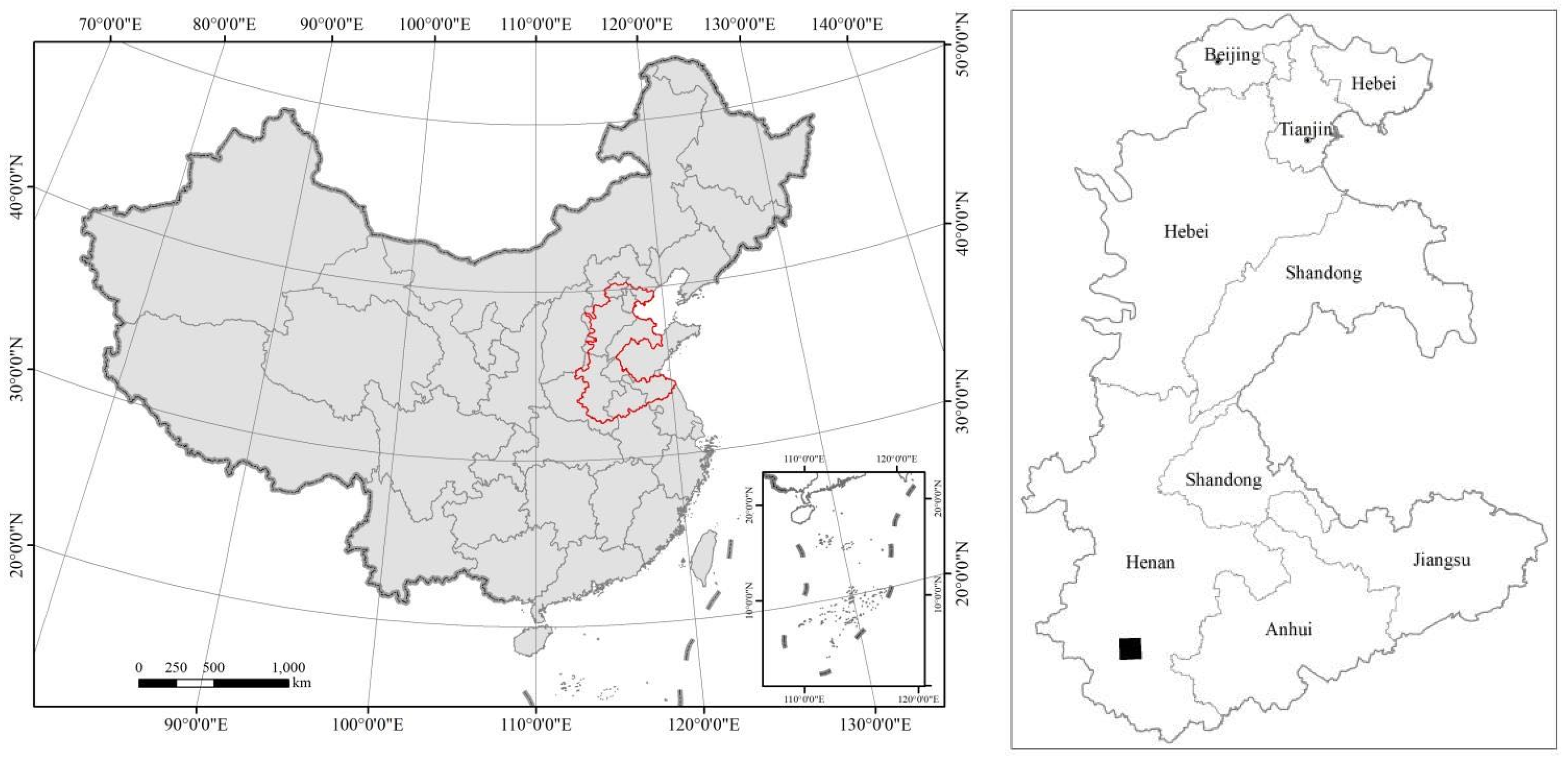
2.1. Study Area

The North China Plain (NCP) (32°14′–40°38′ N, 112°84′–120°33′ E) (Figure 1), which is known as “China’s granary”, provides 40% and 25% of China’s wheat and corn production, respectively, although it only occupies 3.3% of the national area [36]. Geographically, the NCP stretches from the Yanshan Mountains in the north to the mainstream of the Huai River and the primary irrigation canal of Northern Jiangsu in the south. It is bordered by the Taihang and Qinling Mountains in the west and lies adjacent to the Bohai and Yellow Seas in the east. It covers parts or all of Beijing, Tianjin, Hebei, Shandong, Henan, Jiangsu, and Anhui provinces. The NCP has a temperate continental monsoon climate, with an average annual temperature of 13 °C and an average annual precipitation of 710 mm. The deep and fertile soil, combined with appropriate temperature and precipitation, make the NCP highly suitable for the cultivation of crops such as wheat, corn, and soybeans. The dominant grain planting systems in the NCP include winter wheat in the northern region and a winter wheat–summer maize rotation in the southern region. Winter wheat is sown in early- or mid-October and harvested in June of the following year, while summer corn is sown in mid- or late-June and harvested in September of the same year. Consequently, June is the cropland residue burning season in the northern part of the NCP, while both June and October are burning seasons in the southern part of the NCP. For this study, a typical region (highlighted by a black square in Figure 1), covering an area of 30 × 30 km², was selected in Henan Province. Crop burning was previously practiced twice a year in this region until the recent implementation of a local no-burning policy.

2.2. Workflow of Burned-Area Mapping

We employed a combination of the long time-series outlier method and a threshold-optimization algorithm to detect burned areas. The workflow involved the following steps:

(1)

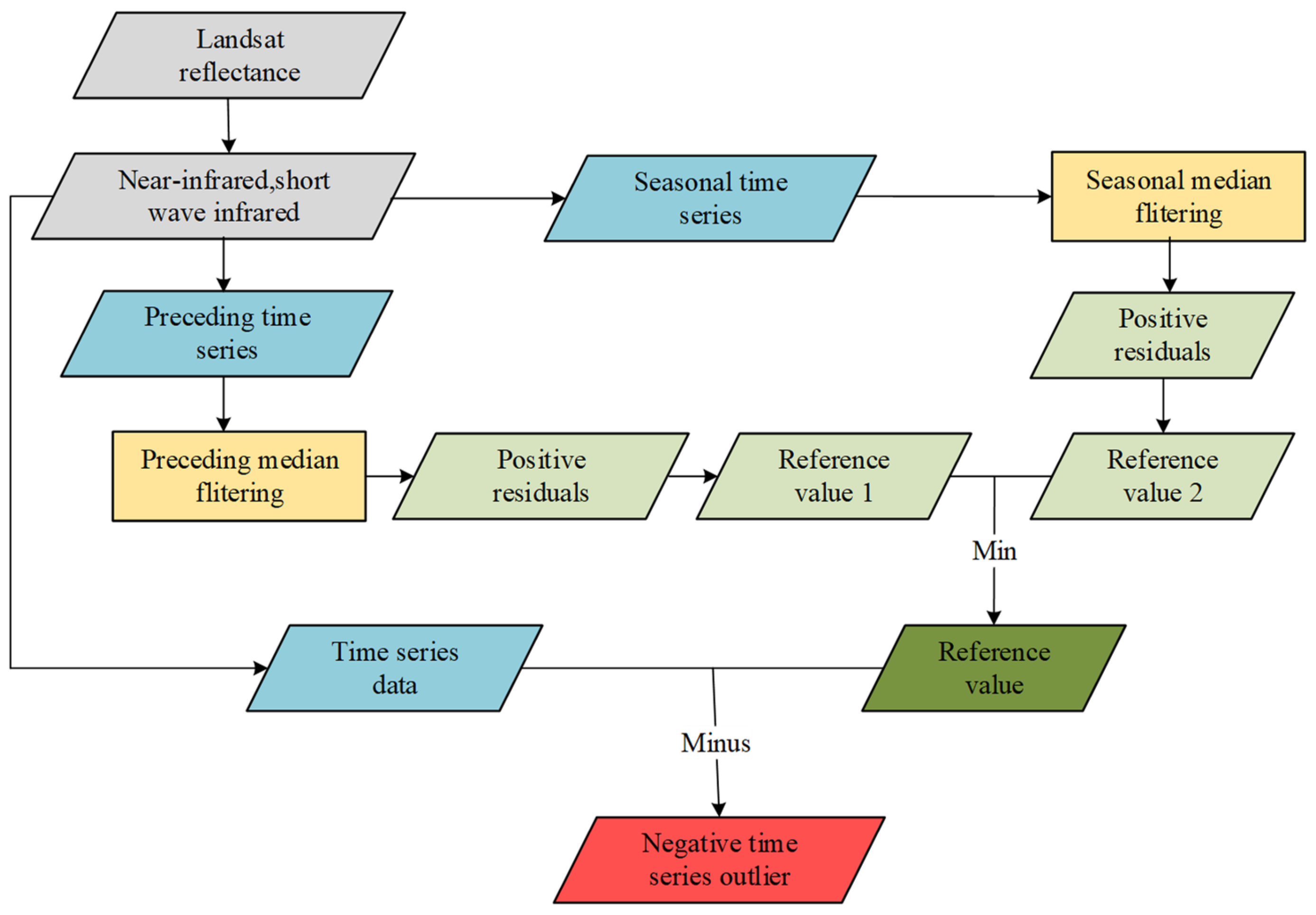
Construction of preceding and seasonal time series: Time-series data were organized to capture the temporal variation in reflectance. This involved constructing the preceding time series, which reflects changes before and after burning events, and the seasonal time series, which captures seasonal variations.

(2)

Calculation of time-series outliers: Outliers in the time series were determined by calculating two reference values through the application of median filtering to each of the constructed time series.

(3)

Determination of the optimal threshold: An iterative procedure was implemented to determine the optimal threshold. This involved systematic iteration through various threshold combinations to identify the threshold value yielding the best results.

(4)

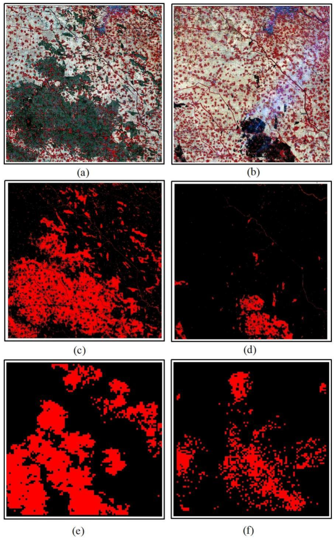
Extraction of cropland burned pixels: The logical relationship between the outliers and optimal threshold was used to extract cropland burned pixels.

All these operations were carried out on the Google Earth Engine (GEE) platform, which provides abundant capacity for data storage and processing. The use of GEE facilitates the efficient handling of large datasets and enables the execution of complex algorithms.

2.2.1. Time-Series Construction

The temporal behavior of harvesting or burning of cropland is characterized by a sudden decline and gradual recovery of spectral values, as well as periodic variations from year to year [16]. To capture these patterns, we constructed two time series: a preceding time series and a seasonal time series. The former is suited to pixels exhibiting long-term and non-seasonal trends. In contrast, the latter is better suited to pixels exhibiting highly periodic and seasonal trends. After a fire occurrence, the reflectance in the NIR and SWIR bands, specifically B4 (TM 4), B5 (TM 5), and B7 (TM 7) of Landsat 5, generally shows a decline [27]. Additionally, Hawbaker et al. [22] found that burn probability is negatively correlated with the short-wave middle infrared (TM 5) band, and positively correlated with the long-wave middle infrared (TM 7) band. On the basis of these findings, B4 and B5 were selected for cropland burned-area detection in this study.

To construct the preceding time series, seven images that were closest to the target image were chosen. Goodwin and Collett [27] found that selecting the seven nearest images strikes a good balance between characterizing unburned reflectance variation and avoiding the inclusion of pixels affected by past burn events. Moreover, to ensure consistency, these seven images must be captured within the same year to eliminate potential cross-year influences on the sequential data.

For the construction of the seasonal time series, it is crucial to ensure that images are captured under comparable growing conditions. Therefore, a progressive search approach was adopted. The specific sampling strategy was as follows:

(1)

The solar azimuth angle and solar altitude angle of the target image were denoted as Azimuth0 and Zenith0, respectively.

(2)

Images were selected based on the criteria that the solar azimuth angle must fall within the interval range [Azimuth0 −15°, Azimuth0 −3°] and [Azimuth0 +3°, Azimuth0 +15°], while the solar altitude angle must be within the range [Zenith0 −15°, Zenith0 −3°] and [Zenith0 +3°, Zenith0 +15°]. Additionally, care was taken to avoid selecting images that were too similar to the target image in terms of seasonal characteristics. Therefore, the selected image and the target image must be within a 60-day interval to capture the desired seasonal spectral changes. This sampling strategy aims to include as many time-series datasets as possible to reflect the variation in surface reflectance.

2.2.2. Time-Series Outlier Detection

Land surface reflectance can be influenced by various factors other than burn characteristics. To mitigate the impact of these factors and focus on burn-related changes, median filtering was employed to calculate the time-series outliers.

First, median filtering was performed on the time-series data (including both the preceding time series and seasonal time series), as shown in Equations (1) and (2).

$$B{45}_{PM}=\mathrm{median}(B{45}_{t-7,}B{45}_{t-6}\dots \dots B{45}_{t-1})$$

(1)

$$B{4}_{PM}=\mathrm{median}(B{4}_{t-7,}B{4}_{t-6}\dots \dots B{4}_{t-1})$$

(2)

In Equation (1), t represents the burning date. The median was computed using the reflectance values of B4 and B45 (sum of B4 and B5) of the seven adjacent images before the burning data.

Second, the difference between the time-series data and the median value was calculated for each time series. A result greater than zero was retained, and a result less than zero was discarded. Then, the average of the “greater than zero” values was calculated. Equations (3)–(5) explain these operations for the preceding time series.

$$R_{PM}=B{45}_t-B{45}_{PM}$$

(3)

$$R_{PM}^P=R_{PM}|R_P>=0$$

(4)

$${\stackrel{⌢}{R}}_{PM}^P=\mathrm{average}(R_{PM}^P)$$

(5)

According to the above method, the seasonal time series was calculated using Equations (6)–(8).

$$R_{SM}=B{45}_t-B{45}_{SM}$$

(6)

$$R_{SM}^P=R_{SM}|R_P>=0$$

(7)

$${\overline{R}}_{SM}^P=\mathrm{average}(R_{SM}^P)$$

(8)

The mean values of the above two time series were taken as interim reference values.

Finally, the smaller of the above two reference values was used as the final reference value (Equation (9)). The difference between the target image and reference image was calculated to obtain the B45 outlier image (Equation (10)).

$$B{45}_{\mathrm{reference}}{=\min (\overline{\mathrm{R}}}_{PM}^P,{\overline{\mathrm{R}}}_{SM}^P)$$

(9)

$$B{45}_{\mathrm{outlier}}=B{45}_{\mathrm{reference}}-B45$$

(10)

According to the above method, the B4 outlier image was calculated using Equations (11) and (12).

$$B{4}_{\mathrm{reference}}{=\min (\overline{\mathrm{R}}}_{PM}^P,{\overline{\mathrm{R}}}_{SM}^P)$$

(11)

$$B{4}_{\mathrm{outlier}}=B{4}_{\mathrm{reference}}-B4$$

(12)

By performing median filtering and calculating time-series outliers, our analysis could focus on the substantial changes associated with burn characteristics while minimizing the influence of factors such as cloud and cloud shadows. The flow chart presented in Figure 2 illustrates the sequential steps involved in this process.

2.2.3. Optimal Threshold Determination and Burned-Area Detection

The cropland burned area can be obtained by comparing the outlier image obtained above with an appropriate threshold; thus, it is crucial to obtain the optimal threshold, as shown in Equation (13).

$$(B{45}_{\mathrm{outlier}}<B{45}_{\mathrm{threshold}}) \mathrm{And} (B{4}_{\mathrm{outlier}}<B{4}_{\mathrm{threshold}})$$

(13)

where, B45_threshold and B4_threshold are the optimal thresholds of B45 and B4, respectively. A pixel satisfying Equation (13) is identified as a burned-area pixel.

To obtain the optimal threshold, we utilized an iterative algorithm, as shown in Figure 3. The specific steps of the threshold iterative algorithm were as follows:

(1)

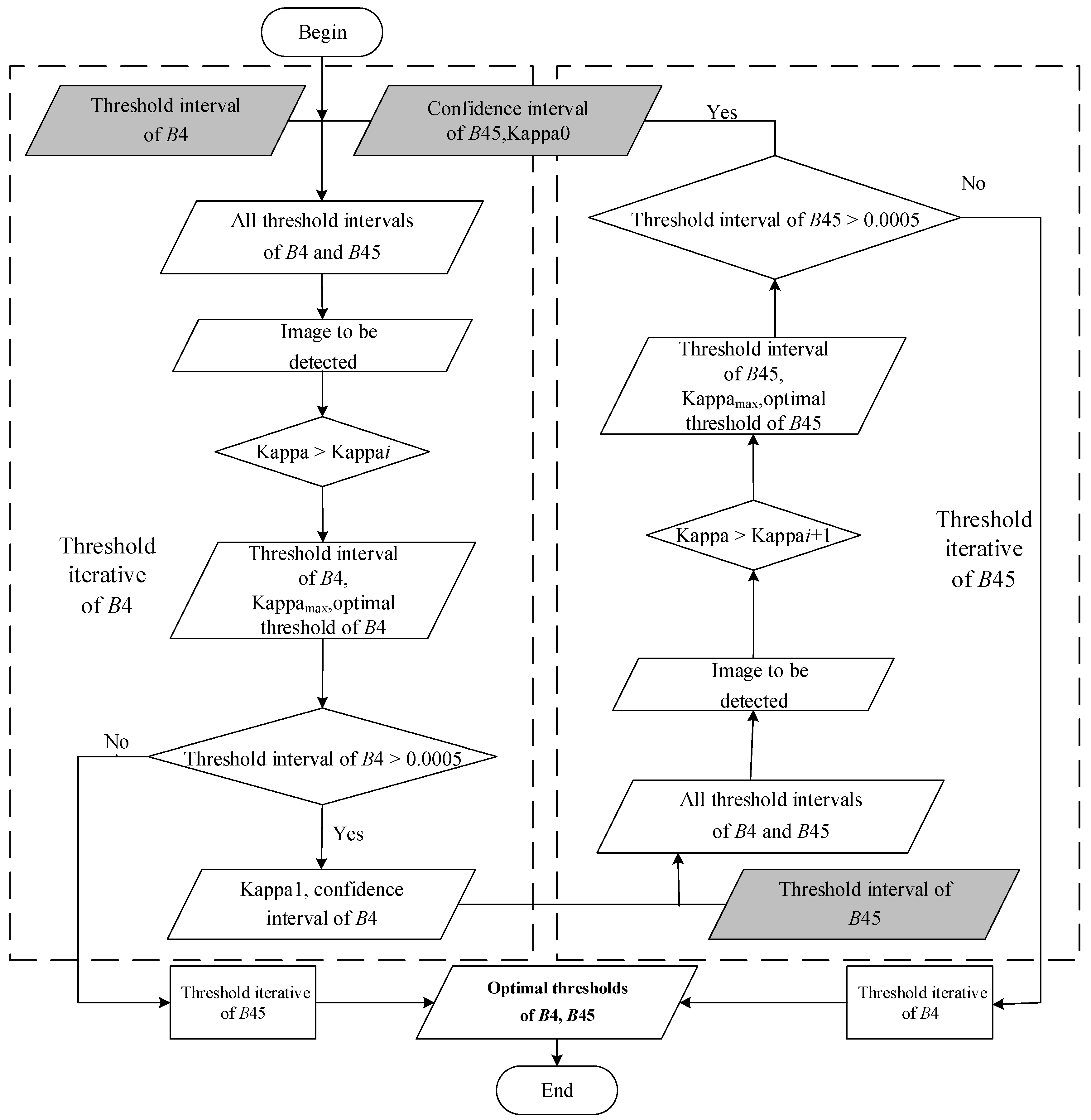
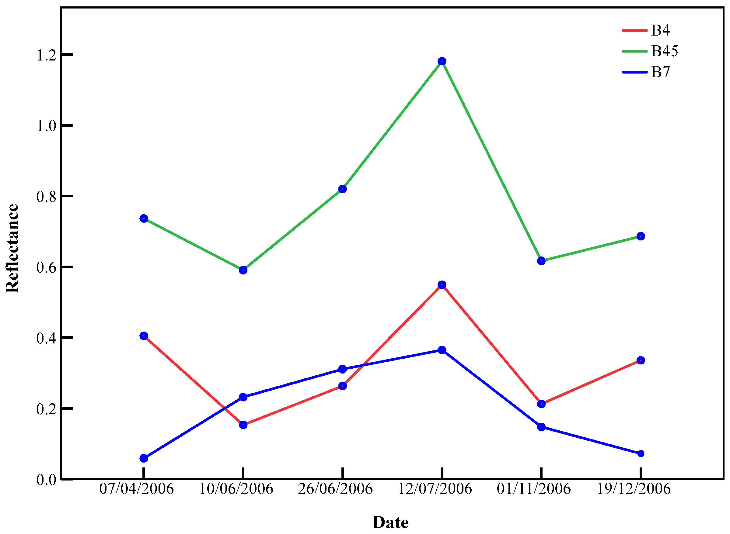
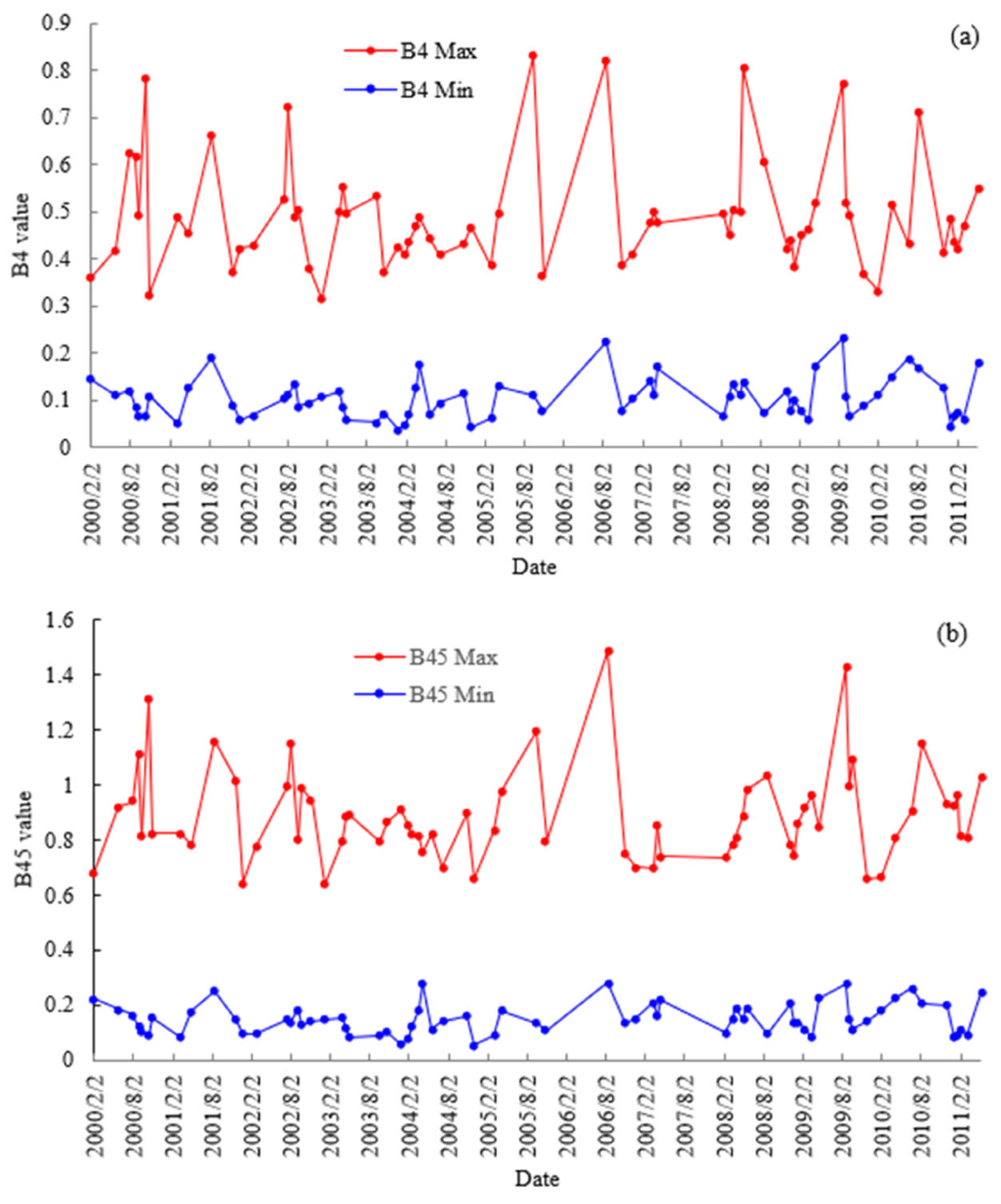
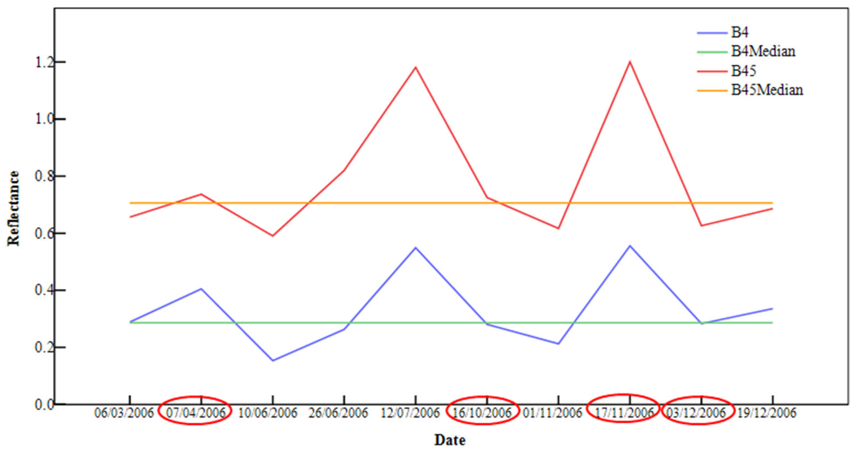
We determined the threshold interval, i.e., the upper and lower bounds of the threshold, through analysis of the time series and calculation of the range. Specifically, the reflectance change curves (maximum and minimum values) for all B4 and B45 images within the time series were plotted, and reasonable upper and lower thresholds were set based on the distribution of these values. Changes in the minimum and maximum values were used to determine the lower and upper thresholds, respectively.

(2)

We initialized six parameters for the iteration, including threshold lower bound, threshold upper bound (for both B45 and B4), kappa coefficient (kappa), and confidence threshold corresponding to the dark gray area in Figure 3. Each iteration required four input parameters: threshold lower bound, threshold upper bound, kappa, and confidence threshold. The output included the updated threshold lower bound, threshold upper bound, kappa, and optimal threshold.

(3)

The kappa and optimal threshold values obtained in each iteration were used as input parameters for the next iteration. Except for the first and second iterations, the threshold interval in the input parameters of the 2nd *i iteration corresponded to the threshold interval in the output parameters of the 2nd *i − 2 iteration. Similarly, the threshold interval in the input parameters of the 2nd *i − 1 iteration corresponded to the threshold interval in the output parameters of the 2nd *i − 3 iteration, where i is a natural number ≥2.

(4)

Kappa was recalculated in each iteration. If the calculated kappa was larger than the reference kappa, the corresponding threshold interval was retained. Simultaneously, this kappa and optimal threshold were retained as input parameters for the next iteration. The range of the threshold interval was gradually reduced if the current kappa was >Kappai. The iteration continued until the range of the threshold interval was <0.0005. It is important to note that the entire iteration procedure was completed by an extra B4 or B45 threshold iteration.

Table 1. The parameters of the threshold-optimization iteration program. Note that the parameters outline the details of the iteration; those in standard font indicate an initial value of the program, those underlined indicate an intermediate output of the program, and those double underlined indicate the optimal thresholds calculated by the program.

ID	Threshold Lower Bound	Threshold Upper Bound	Kappai	Confidence Threshold	Threshold Lower Bound	Threshold Upper Bound	Kappai + 1	Optimal Threshold
1	B4min	B4max	Kappa0	B45T0	B4min1	B4max1	Kappa1	B4T1
2	B45min	B45max	Kappa1	B4T1	B45min2	B45max2	Kappa2	B45T2
3	B4min1	B4max1	Kappa2	B45T2	B4min3	B4max3	Kappa3	B4T3
4	B45min2	B45max2	Kappa3	B4T3	B45min4	B45max4	Kappa4	B45T4
5	B4min3	B4max3	Kappa4	B45T4	B4min5	Band4max5	Kappa5	B4T5

provides the specific iteration parameters used in the threshold-optimization program.

3. Results

3.1. Time-Series Outliers

For this study, the target image was acquired on 10 June 2006. To construct the preceding time series, images from corresponding adjacent dates with cloud cover <50% were selected. Specifically, the preceding time series consisted of images acquired on 7 April, 26 June, 12 July, 1 November, and 19 December, respectively. This preceding time-series period was 257 days. Additionally, a total of 107 images that met the conditions for constructing the seasonal time series were selected.

Figure 4 shows the spectral variation characteristics of the three utilized bands (TM4, TM5, and TM7) before and after crop-straw burning in 2006. Through visual interpretation of the satellite imagery, we found that this area exhibited post-burning characteristics on 1 November 2006.

The reflectance values of TM4 (B4) and the sum of the reflectance values of TM4 and TM5 (B45) exhibited substantial changes before and after 1 November 2006. The B4 values showed a substantial decrease from 0.55 to 0.21, while B45 decreased from 1.18 to 0.61. However, with the implementation of new crop cultivation, these two values increased, reaching 0.34 and 0.69, respectively. In contrast, the reflectance of TM7 (B7) showed irregular changes owing to the burning and sowing of new crops. Therefore, using B7 or an index incorporating B7 to detect cropland burning would lead to a high error. Hence, we selected B4 and B45 as the spectral bands to detect burned areas, rather than relying on B7.

3.2. Optimal Threshold

3.2.1. Threshold Interval Determination

To obtain the optimal threshold, we employed an iterative procedure; in this, it is crucial to set reasonable initial values for the threshold interval. The choice of the threshold interval for B4 and B45 not only affects the number of iterations required but also impacts the accuracy of the optimal threshold result. To determine the threshold interval, statistical analysis of the reflectance values of B4 and B45 from all 107 data images was conducted (as depicted in Figure 5). This analysis revealed the range of maximum and minimum reflectance values for both bands.

For B4, we observed that the maximum reflectance values exhibited a wide range, fluctuating between 0.3 and 0.9. However, the majority of these values were <0.6. Meanwhile, the minimum reflectance values ranged from 0.03 to 0.25, with most being <0.15. Based on this analysis, a reasonable threshold interval for B4 was set as [0.1, 0.6]. For B45, the maximum reflectance values fluctuated between 0.6 and 1.5, with a concentration of values between 0.6 and 1.0. Meanwhile, the minimum reflectance values ranged from 0.0 to 0.3, with most being <0.25. Therefore, a reasonable threshold interval for B45 was determined as [0.2, 1.0].

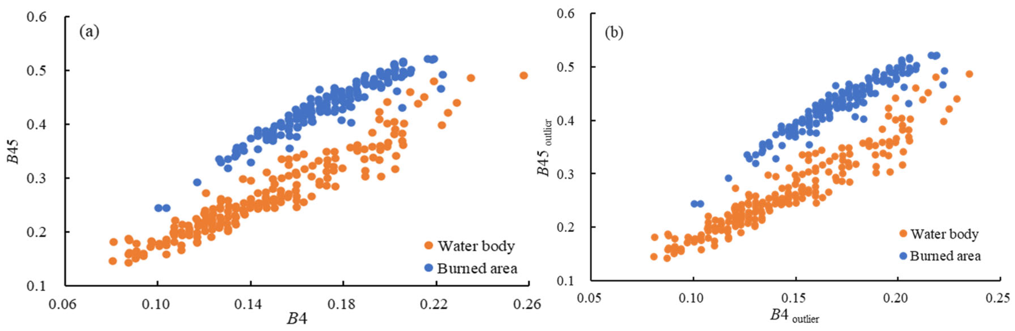
3.2.2. Sampling Points for Threshold Optimization

To optimize the thresholds, it is crucial to obtain a representative sample of burned pixels. Herein, a total of 800 points were selected for this purpose. The selection process involved two main steps, threshold optimization and detection accuracy evaluation.

For threshold optimization, two sets of 200 random points were chosen to determine the optimal threshold for two specific dates, respectively, namely 10 June 2006 and 8 June 2011. These dates were selected to represent different time periods and enable the evaluation of threshold performance across different years.

For detection accuracy evaluation, another two sets of 200 random points were selected to assess the accuracy of the optimal threshold for 10 June 2006 and 8 June 2011, respectively. These points were used to verify the performance of the threshold in correctly identifying burned pixels.

In both steps, the selected sampling points were visually interpreted to determine whether they corresponded to burned pixels or unburned pixels.

3.2.3. Optimal Threshold Iteration

In Section 3.2.1, the threshold interval for the B4 reflectance value was defined as [0.1, 0.6], while that for the B45 reflectance value was set as [0.2, 1.0]. It is important to note that the threshold interval for B4 was smaller than that for B45. Additionally, the reflectance values of B4 were generally relatively lower than those of B45. Considering these factors, the iterative process of threshold optimization proceeded by first conducting the iteration for the B4 threshold interval, as indicated in the flow chart in Figure 3. This sequence was implemented to address the potential uncertainties associated with the higher reflectance values of B45 when combined with the lower values of B4.

The parameters and results of the threshold values of the iterative process for the target image on 10 June 2006 are shown in

Table 2. The iterative process and results of threshold value calculation for the target image on 10 June 2006. Note that values in standard font indicate an initial value of the program, those underlined indicate an intermediate output of the program, and those double underlined indicate the optimal thresholds calculated by the program, those in italics indicate the threshold of lower and upper bounds, given by the iteration.

ID	Threshold Lower Bound	Threshold Upper Bound	Kappai	Confidence Threshold	Threshold Lower Bound	Threshold Upper Bound	Kappai + 1	Optimal Threshold
1	1000	6000	0	5000	1000	6000	0.785	2020.408
2	2000	10,000	0.785	2020.408	5102.041	10,000	0.811	5561.224
3	1000	6000	0.811	5561.224	2020.408	2122.449	0.812	2122.449
4	5102.041	10,000	0.812	2122.449	5501.874	5501.874	0.812	5501.874
5	2020.408	2122.449	0.812	5501.874	2022.491	2122.449	0.820	2030.820

. The number of threshold iterations was small, thus reducing any unnecessary calculation. In addition, the B4 threshold interval converged slowly, while the B45 threshold interval converged quickly. Crucially, the optimal threshold calculated in the previous iteration was used as the confidence threshold and the kappa was used as the parameter for narrowing the threshold interval. Consequently, the threshold interval converged quickly. This iterative program showed high convergence speed and processing efficiency.

To verify the effectiveness of the iterative procedure, cropland burning in the study area on 8 June 2011 was also detected. The threshold iteration process and results of the optimal threshold calculation for this date are shown in

Table 3. The iterative process and results of threshold value calculation for the target image on 8 June 2011. Note that values in standard font indicate an initial value of the program, those underlined indicate an intermediate output of the program, and those double underlined indicate the optimal thresholds calculated by the program, those in italics indicate the threshold of lower and upper bounds, given by the iteration.

ID	Threshold Lower Limit	Threshold Upper Limit	Kappai	Confidence Threshold	Threshold Lower Limit	Threshold Upper Limit	Kappai + 1	Optimal Threshold
1	1000	6000	0	5000	1000	6000	0.939	1816.327
2	2000	10,000	0.939	1816.327	4183.673	10,000	0.939	4183.673
3	1000	6000	0.939	4183.673	1816.327	2020.408	0.939	1816.327
4	4183.673	10,000	0.939	1816.327	4183.673	10,000	0.939	4183.673
5	1816.327	2020.408	0.939	4183.673	1816.327	2020.408	0.939	1816.327

. Kappa did not change in the iteration process and reached a very high value in the first iteration, but the threshold confidence changed and increased with iteration. Unlike for 10 June 2006, the iterative procedure quickly determined the optimal threshold for this date. This may be related to the different burning characteristics of the two days. In the selected image range, the burned area on 8 June 2011 was relatively small and clustered. This facilitated the iterative procedure to determine the change characteristics of the band value after burning more quickly, further providing the lower and upper bounds of the band and the optimal threshold.

3.2.4. Optimal Threshold Validation

The cropland burned area was obtained by applying Equation (13). To evaluate the accuracy of the results, the sample points used for accuracy analysis of the optimal threshold were utilized.

Table 4. The precision validation results of the optimal threshold accuracy of different sampling methods.

Overall Accuracy	Kappa	Burned Pixel		Unburned Pixel
		Commission Error	Omission Error	Commission Error	Omission Error
93.0%	0.84	13.85%	8.2%	3.7%	6.48%

presents the assessment metrics, including the overall accuracy, kappa, commission error, and omission error. The results demonstrated that the verification accuracy corresponding to the optimal threshold was high. The overall accuracy reached 93% and the kappa was 0.84. Although the commission error for burned pixels was relatively higher, it was still <15%. Based on these findings, we concluded that the optimal threshold obtained through iteration exhibits high confidence and can effectively differentiate between burned-area pixels and unburned-area pixels. The accuracy evaluation results indicate that the threshold-based approach employed herein is reliable for detecting and distinguishing burned areas in croplands.

3.3. Intercomparison of Burned Area and MCD64A1

Figure 6 displays the burned-area maps for the construction method on 10 June 2006 and for the validation on 8 June 2011. To assess the accuracy of cropland burned-area detection, an additional round of uniform sampling was conducted, resulting in a total of 400 sampling points. A comparison between the detection results of this study and those of MCD64A1 is presented in

Table 5. The validation results of the burned area detected herein and that of MCD 64A1.

	Overall Accuracy	Kappa	Burned		Unburned
			Commission Error	Omission Error	Commission Error	Omission Error
MCD64A1	76.5%	0.24	50.90%	69.90%	19.00%	9.45%
Burned area in this paper	93.25%	0.82	18.90%	7.53%	2.38%	6.51%

. Noticeable commission and omission errors occurred in the latter owing to its lower spatial resolution; MCD64A1 misclassified a substantial number of burned pixels as unburned, leading to a high omission error. In terms of overall accuracy and kappa, the algorithm used herein outperformed MCD64A1 in accurately identifying burned areas. Notably, the higher burned-area overall accuracy achieved by our algorithm was particularly advantageous in distinguishing burned pixels from unburned pixels.

Compared with the results of our algorithm, MCD64A1 detected more burned areas, especially on 8 June 2011. Owing to the limitation in spatial resolution of the input sensor of the MCD64A1 product, some mixed pixels (consisting of burned and unburned pixels) may be classified as burned pixels. The algorithm used herein showed strong detection capabilities for small burned areas. The results on 10 June 2006 demonstrate that many small burned patches were detected herein, but were not detected by MCD64A1. Meanwhile, compared with MCD64A1, the burned areas detected herein had finer boundaries. These findings underscore the superiority of the algorithm employed herein when compared with MCD64A1, highlighting its potential for more accurate and reliable detection of burned areas in croplands.

4. Discussion

4.1. Advantages of the Algorithm

Combining time-series change detection and threshold optimization has proved to be an effective means of detecting cropland burned areas. Through accuracy verification and comparative verification with MCD64A1, we consider that our algorithm is suitable for the detection of cropland burned areas. The detection algorithm uses Landsat data, taking advantage of its preferable spatial resolution and spectral information, and overcoming the limitations of MODIS data, which has limited accuracy due to its low spatial resolution [14]. Furthermore, traditional detection algorithms (whether a contextual algorithm based on a relative or absolute threshold, or a detection algorithm based on a spectral index) cannot overcome the influence of the spatial heterogeneity of large areas. Our algorithm uses two different sampling strategies to construct time series; this overcomes the influence of spatial heterogeneity and reduces the probability of misjudgment caused by seasonal or other factors. The overall accuracy of our algorithm reached 93.25%, which is better than current general burned-area products. Therefore, this algorithm is suitable for farmland burned-area detection.

The reasons for the high accuracy of our algorithm can be summarized as follows. (1) Studies have shown that the reflectance values drop most evidently in the NIR and SWIR bands after burning [37]. Herein, good results were achieved using Landsat image NIR and SWIR bands for burning detection [27]. We have shown that using the B4 and B45 reflectance values for burned-area detection gives better results than those using B4 and B7 values when calculating time-series outliers. Therefore, selecting the NIR and SWIR1 of Landsat images as two important parameters for outlier calculation ensures detection accuracy. (2) The seasonal time series adopted herein fully considers the seasonal repetitive characteristics of crop-straw burning, reduces the possibility of low-reflectance pixels caused by non-burning factors being misclassified as burned pixels, and ensures a low commission error of unburned pixels. (3) The Landsat-5 surface reflectance product based on the GEE platform was used herein. This product uses the CFMASK algorithm to detect clouds, achieving good results [38], which greatly reduces the impact of clouds and cloud shadows on fire detection. The accuracy of the product is high, with reflectance values accurate to 0.001, which results in the optimal threshold being more accurate, and improves the detection accuracy.

In addition, the automation of threshold setting is an important problem in the threshold method. Herein, an iterative program was used to realize automatic optimization of the threshold. This avoids time-consuming manual adjustment and also improves the accuracy of cropland burned-area detection. Therefore, this automatic threshold optimization could provide a foundation for future applications of other remote sensing or spectral band data to extract cropland burned areas in larger regions.

4.2. Limitations of the Algorithm

Although good performance was achieved in this study, there are some shortcomings that require further improvement. First, in the construction of the preceding time series, the selection of appropriate reference values can make calculating outliers more conducive to distinguishing burned and unburned areas, and the size of the outliers will further affect threshold optimization. Figure 7 shows the reflectance values and their medians for the preceding time series. It can be seen that the reflectance values of B4 and B45 on four dates (red circles in Figure 7) are abnormal because cloud cover in the images for these days exceeded 50%. A large number of clouds and cloud shadows can result in unusually high (e.g., 17 November 2006) or unusually low (e.g., 3 December 2006) spectral values, respectively. If there are abundant pixels in the time-series data with abnormally low reflectance caused by cloud shadows or other non-burning factors, the median reflectance of this time-series data will be low, and the outliers calculated using the actual burned pixels will be high, causing burned pixels to be misjudged as unburned pixels. Consequently, if the median reflectance value of time-series data under such a sampling strategy is selected as the reference value, the probability of misjudgment will increase. The removal of cloud-contaminated images when constructing the preceding time series resulted in the inadequate representation of the median values and consequential outliers. This limitation of Landsat is offset by the advantage of MODIS, whose higher time resolution (i.e., daily repetition) can ensure the accuracy of the constructed preceding time series and better reflect the annual variation characteristics of cropland burning.

Second, when analyzing the misclassification of burned pixels, we found that a considerable proportion of water pixels were misclassified as burned pixels. Channel TM5 shows different spectral characteristics for recent and aged fire scars, and recent scars in this channel were easily mistaken for water bodies [39]. The pixel_qa band in the surface reflectance data of the GEE platform has a low detection accuracy for water. Because water strongly absorbs in the NIR and SWIR bands, its reflectance value is very low and the outliers calculated from these bands are also low, resulting in misclassification as a burned pixel. To further explore the reasons for the commission errors of water bodies, 232 water-body sampling points (Figure 8) were collected, among which 228 water pixels were mistakenly detected as burned pixels.

Figure 9 shows the B4 and B45 reflectance values (Figure 9a) and B4_outlier and B45_outlier values (Figure 9b) of water-body sampling points and burned pixels. The B4 and B45 reflectance values of the water-body sampling points misclassified as burned pixels were lower than those of true burned pixels. Similarly, the B4_outlier and B45_outlier values of the water-body sampling points misclassified as burned pixels were lower than those of true burned pixels. The water-body sampling points were more dispersed than the burned pixels both in terms of their reflectance values and outliers. In general, the outliers of the water-body sampling points and burned pixels were more dispersed than the corresponding reflectance values. However, the water-body areas were small and difficult to detect when visually interpreting the image, so this algorithm does not further detect the water bodies.

4.3. Future Directions and Recommendations

The use of time-series analysis to characterize temporal trends in reflectance facilitated the automation of our algorithm by improving the discrimination of fire-related changes from seasonal and non-seasonal influences on vegetation. When constructing the preceding time series, it is necessary to collect seven images adjacent to the detection date, and the cloud cover of these images is required to meet a given standard. However, the number of available images is insufficient owing to the relatively low temporal resolution of Landsat data. Furthermore, in contrast to wildfires in rangeland and forests, crop-straw burning has more frequent changes within a year, and fires in cropland are commonly of a short duration [16]. For example, crop-straw burning occurred twice in the year studied herein; vegetation recovery is usually quite quick after a fire, and the temporal gaps usually result in a high omission error. Consequently, on the one hand, it is essential that denser time series are gathered for cropland burned-area detection, but on the other hand, it is difficult to construct such time series only using Landsat data. This problem can be solved in two ways: (1) further experiments should be carried out to determine the characteristics of the annual spectral variation of cropland burning, and a more appropriate number of images should be selected to construct the preceding time series; (2) imagery with higher temporal resolution should be chosen or the synergy of multiple data sources should be used to obtain denser time series.

To improve the accuracy of this algorithm further, it could be used in combination with other burned-area detection algorithms. In this study, we adopted an algorithm combining an improved spectral index and positive points excluded using the SWIR and thermal infrared bands of Landsat 8 for fire detection [40]. It is known that the temperature of water bodies is lower than that of land after burning [27]. Hence, in future studies, the thermal infrared band could be used to remove false burned pixels. Likewise, the contextual fire-point detection algorithm could be used to exclude most false detection points located in water bodies and residential areas to improve detection accuracy. Moreover, the JRC Monthly Water History dataset provided by the GEE platform contains accurate maps of the location and temporal distribution of surface water. If this dataset were to be used for mask processing, the detection accuracy could also be improved in the future.

In addition to the aforementioned issues, it is important to address another concern. This paper exclusively focused on evaluating the algorithm’s effectiveness in a representative farmland in the NCP region of China, where farmland burning is common. However, for a more comprehensive assessment, it would be essential to include diverse experimental sites covering various crop types. Future studies could incorporate additional test areas spanning different crop types to facilitate a more comprehensive verification process of the algorithm.

5. Conclusions

Existing burned-area detection methods based on band values and spectral indices are limited by their subjectivity and low efficiency in determining outliers and thresholds. In this paper, we proposed an automatic algorithm combined with a threshold-optimization method based on two time series utilizing the GEE platform. We took an area of Henan Province on the NCP as our study area to examine the applicability of the proposed method. In contrast to previous coarse-resolution burned-area products, the burned-area map was derived from all available Landsat images, and its commission and omission errors were 18.9% and 7.53%, respectively. This high detection accuracy is attributed to the use of two time series that together can fully consider the annual and seasonal variations in cropland burning. Meanwhile, the automatic threshold-optimization algorithm improves the detection efficiency and more accurately expresses the time-series outliers of burning characteristics. In summary, this study could provide several routes for the future application of other remote-sensing or spectral-band data to extract cropland burned areas in larger regions.

References

1. Chang, C.H.; Liu, C.C.; Tseng, P.Y. Emissions Inventory for Rice Straw Open Burning in Taiwan Based on Burned Area Classification and Mapping Using Formosat-2 Satellite Imagery. Aerosol Air Qual. Res. 2013, 13, 474–487. [Google Scholar] [CrossRef]
2. Chen, D.; Loboda, T.V.; He, T.; Zhang, Y.; Liang, S. Strong cooling induced by stand-replacing fires through albedo in Siberian larch forests. Sci. Rep. 2018, 8, 4821. [Google Scholar] [CrossRef] [PubMed]
3. López-Saldaña, G.; Bistinas, I.; Pereira, J.M.C. Global analysis of radiative forcing from fire-induced shortwave albedo change. Biogeosciences 2015, 12, 557–565. [Google Scholar] [CrossRef]
4. Ward, D.S.; Kloster, S.; Mahowald, N.M.; Rogers, B.M.; Randerson, J.T.; Hess, P.G. The changing radiative forcing of fires: Global model estimates for past, present and future. Atmos. Chem. Phys. 2012, 12, 10857–10886. [Google Scholar] [CrossRef]
5. Stavrakoudis, D.; Katagis, T.; Minakou, C.; Gitas, I.Z. Towards a fully automatic processing chain for operationally mapping burned areas countrywide exploiting Sentinel-2 imagery. In Proceedings of the Seventh International Conference on Remote Sensing and Geoinformation of the Environment (RSCy2019), International Society for Optics and Photonics, Paphos, Cyprus, 18–21 March 2019; Volume 11174, p. 1117405. [Google Scholar]
6. van Dijk, D.; Shoaie, S.; Leeuwen, T.V.; Veraverbekea, S. Spectral signature analysis of false positive burned area detection from agricultural harvests using Sentinel-2 data. Int. J. Appl. Earth. Obs. Geoinf. 2021, 97, 102296. [Google Scholar] [CrossRef]
7. Liu, P.; Liu, Y.; Guo, X.; Zhao, W.; Wu, H.; Xu, W. Burned area detection and mapping using time series Sentinel-2 multispectral images. Remote Sens. Environ. 2023, 296, 113753. [Google Scholar] [CrossRef]
8. Bastarrika, A.; Chuvieco, E.; Martín, M.P. Automatic burned land mapping from MODIS time series images: Assessment in Mediterranean ecosystems. IEEE Trans. Geosci. Remote Sens. 2011, 49, 3401–3413. [Google Scholar] [CrossRef]
9. Chuvieco, E.; Roteta, E.; Sali, M.; Stroppiana, D.; Boettcher, M.; Kirches, G.; Storm, T.; Khairoun, A.; Pettinari, M.L.; Franquesa, M.; et al. Building a small fire database for Sub-Saharan Africa from Sentinel-2 high-resolution images. Sci. Total Environ. 2022, 845, 157139. [Google Scholar] [CrossRef]
10. Ramo, R.; Roteta, E.; Bistinas, I.; Van Wees, D.; Bastarrika, A.; Chuvieco, E.; Van der Werf, G.R. African burned area and fire carbon emissions are strongly impacted by small fires undetected by coarse resolution satellite data. Proc. Natl. Acad. Sci. USA 2021, 118, e2011160118. [Google Scholar] [CrossRef]
11. Pinto, M.M.; Libonati, R.; Trigo, R.M.; Trigo, I.F.; DaCamara, C.C. A deep learning approach for mapping and dating burned areas using temporal sequences of satellite images. ISPRS J. Photogramm. Remote Sens. 2020, 160, 260–274. [Google Scholar] [CrossRef]
12. Roteta, E.; Bastarrika, A.; Ibisate, A.; Chuvieco, E. A preliminary global automatic burned-area algorithm at medium resolution in Google Earth Engine. Remote Sens. 2021, 13, 4298. [Google Scholar] [CrossRef]
13. Libonati, R.; DaCamara, C.C.; Setzer, A.W.; Morelli, F.; Melchiori, A.E. An algorithm for burned area detection in the Brazilian Cerrado using 4 µm MODIS imagery. Remote Sens. 2015, 7, 15782–15803. [Google Scholar] [CrossRef]
14. Zhu, C.; Kobayashi, H.; Kanaya, Y.; Saito, M. Size-dependent validation of MODIS MCD64A1 burned area over six vegetation types in boreal Eurasia: Large underestimation in croplands. Sci. Rep. 2017, 7, 4181. [Google Scholar] [CrossRef] [PubMed]
15. Wang, Y.; Xin, L.; Zhang, H.; Li, Y. An estimation of the extent of rent-free farmland transfer and its driving forces in rural China: A multilevel logit model analysis. Sustainability 2019, 11, 3161. [Google Scholar] [CrossRef]
16. Long, T.; Zhang, Z.; He, G.; Jiao, W.; Tang, C.; Wu, B.; Zhang, X.; Wang, G.; Yin, R. 30 m resolution global annual burned area mapping based on Landsat Images and Google Earth Engine. Remote Sens. 2019, 11, 489. [Google Scholar] [CrossRef]
17. Hawbaker, T.J.; Vanderhoof, M.K.; Schmidt, G.L.; Beal, Y.J.; Picotte, J.J.; Takacs, J.D.; Falgout, J.T.; Dwyer, J.L. The Landsat Burned Area algorithm and products for the conterminous United States. Remote Sens. Environ. 2020, 244, 111801. [Google Scholar] [CrossRef]
18. Boschetti, L.; Flasse, S.; Trigg, S.; de Dixmude, A.J. A multitemporal change-detection algorithm for the monitoring of burnt areas with SPOT-Vegetation data. In Analysis of Multi-Temporal Remote Sensing Images; World Scientific Publishing: Singapore, 2002; pp. 75–82. [Google Scholar]
19. Schroeder, W.; Oliva, P.; Giglio, L.; Quayle, B.; Lorenz, E.; Morelli, F. Active fire detection using Landsat-8/OLI data. Remote Sens. Environ. 2016, 185, 210–220. [Google Scholar] [CrossRef]
20. Lizundia-Loiola, J.; Otón, G.; Ramo, R.; Chuvieco, E. A spatio-temporal active-fire clustering approach for global burned area mapping at 250 m from MODIS data. Remote Sens. Environ. 2020, 236, 111493. [Google Scholar] [CrossRef]
21. Bastarrika, A.; Alvarado, M.; Artano, K.; Martinez, M.P.; Mesanza, A.; Torre, L.; Ramo, R.; Chuvieco, E. BAMS: A tool for supervised burned area mapping using Landsat data. Remote Sens. 2014, 6, 12360–12380. [Google Scholar] [CrossRef]
22. Hawbaker, T.J.; Vanderhoof, M.K.; Beal, Y.J.; Takacs, J.D.; Schmidt, G.L.; Falgout, J.T.; Williams, B.; Fairau, N.M.; Caldwell, M.K.; Picotte, J.J.; et al. Mapping burned areas using dense time-series of Landsat data. Remote Sens. Environ. 2017, 198, 504–522. [Google Scholar] [CrossRef]
23. Liu, J.; Heiskanen, J.; Maeda, E.E.; Pellikka, P.K.E. Burned area detection based on Landsat time series in savannas of southern Burkina Faso. Int. J. Appl. Earth Obs. Geoinf. 2018, 64, 210–220. [Google Scholar] [CrossRef]
24. Ruscalleda-Alvarez, J.; Moro, D.; Van Dongen, R. A multi-scale assessment of fire scar mapping in the Great Victoria Desert of Western Australia. Int. J. Wildland Fire 2021, 30, 886–898. [Google Scholar] [CrossRef]
25. Wei, M.; Zhang, Z.; Long, T.; He, G.; Wang, G. Monitoring Landsat based burned area as an indicator of Sustainable Development Goals. Earth’s Future 2021, 9, e2020EF001960. [Google Scholar] [CrossRef]
26. Pereira, M.C.; Setzer, A.W. Spectral characteristics of fire scars in Landsat-5 TM images of Amazonia. Remote Sens. 1993, 14, 2061–2078. [Google Scholar] [CrossRef]
27. Goodwin, N.R.; Collett, L.J. Development of an automated method for mapping fire history captured in Landsat TM and ETM+ time series across Queensland, Australia. Remote Sens. Environ. 2014, 148, 206–221. [Google Scholar] [CrossRef]
28. Mor, S.; Singh, T.; Bishnoi, N.R.; Bhukal, S.; Ravindra, K. Understanding seasonal variation in ambient air quality and its relationship with crop residue burning activities in an agrarian state of India. Environ. Sci. Pollut. Res. 2022, 29, 4145–4158. [Google Scholar] [CrossRef] [PubMed]
29. Chen, W.; Moriya, K.; Sakai, T.; Koyama, L.; Cao, C.X. Mapping a burned forest area from Landsat TM data by multiple methods. Geomat. Nat. Hazards Risk 2014, 7, 384–402. [Google Scholar] [CrossRef]
30. Woźniak, E.; Aleksandrowicz, S. Self-Adjusting Thresholding for Burnt Area Detection Based on Optical Images. Remote Sens. 2019, 11, 2669. [Google Scholar] [CrossRef]
31. Filipponi, F. Exploitation of Sentinel-2 Time Series to Map Burned Areas at the National Level: A Case Study on the 2017 Italy Wildfires. Remote Sens. 2019, 11, 622. [Google Scholar] [CrossRef]
32. Zhang, S.; Zhang, Y.; Zhao, H. Integration of Multiple Spectral Data via a Logistic Regression Algorithm for Detection of Crop Residue Burned Areas: A Case Study of Songnen Plain, Northeast Chin. Chin. Geogr. Sci. 2024, 34, 548–563. [Google Scholar] [CrossRef]
33. Stroppiana, D.; Bordogna, G.; Carrara, P.; Boschetti, M.; Boschetti, L.; Brivio, P.A. A method for extracting burned areas from Landsat TM/ETM+ images by soft aggregation of multiple Spectral Indices and a region growing algorith. ISPRS J. Photogramm. Remote Sens. 2012, 69, 88–102. [Google Scholar] [CrossRef]
34. Storey, E.A.; Lee West, K.R.; Stow, D.A. Utility and optimization of LANDSAT-derived burned area maps for southern California. Int. J. Remote Sens. 2021, 42, 486–505. [Google Scholar] [CrossRef]
35. Koutsias, N.; Pleniou, M.; Mallinis, G.; Nioti, F.; Sifakis, N.I. A rule-based semi-automatic method to map burned areas: Exploring the USGS historical Landsat archives to reconstruct recent fire history. Int. J. Remote Sens. 2013, 34, 7049–7068. [Google Scholar] [CrossRef]
36. Zhang, Y.; Dore, A.J.; Ma, L.; Liu, X.J.; Ma, W.Q.; Cape, J.N.; Zhang, F.S. Agricultural ammonia emissions inventory and spatial distribution in the North China Plain. Environ. Pollut. 2010, 158, 490–501. [Google Scholar] [CrossRef] [PubMed]
37. Key, C.H.; Benson, N.C. Measuring and remote sensing of burn severity: The CBI and NBR. In Proceedings of the Joint Fire Science Conference and Workshop, Boise, ID, USA, 15–17 June 1999; Volume 2000, pp. 284–285. [Google Scholar]
38. Beckmann, T.; Schmidt, G.L.; Dwyer, J.L.; Hughes, M.J.; Laue, B. Cloud detection algorithm comparison and validation for operational Landsat data products. Remote Sens. Environ. 2017, 194, 379–390. [Google Scholar]
39. Pereira, J.M.; Sá, A.C.; Sousa, A.M.; Silva, J.M.; Santos, T.N.; Carreiras, J.M. Spectral characterisation and discrimination of burnt areas. In Remote Sensing of Large Wildfires; Springer: Berlin/Heidelberg, Germany, 1999; pp. 123–138. [Google Scholar]
40. He, Y.; Yang, J.; Ma, Y.; Liu, J.B.; Chen, F.; Li, X.P.; Yang, Y.F. A method for fire detection using Landsat 8 data. J. Infrared Millim. Waves 2016, 35, 600–609. [Google Scholar]
Figure 1. The study area location. The left figure depicts the boundaries of China; the right figure represents the North China Plain (NCP) bound and the provinces included. The black area in the right figure represents the algorithm evaluation area selected in this paper.
Fire 07 00257 g001
Figure 2. The workflow of time-series outlier detection. The gray panels represent raw data, the other colored panels represent intermediate steps in the outlier calculation, and the red panel represents the final outlier.
Fire 07 00257 g002
Figure 3. A flow chart of the optimal threshold iterative program.
Fire 07 00257 g003
Figure 4. The reflectance change of pixels (33.26° N, 114.5584° E) in the preceding time series of 2006.
Fire 07 00257 g004
Figure 5. The maximum and minimum reflectance values of (a) Band 4 (B4) and (b) Band 45 (B45).
Fire 07 00257 g005
Figure 6. A comparison of burned-area detection results. (a,b) A TM image in RGB: 432 on 10 June 2006 and 8 June 2011, respectively. (c,d) Burned area detected herein on 10 June 2006 and 8 June 2011, respectively. (e,f) MCD64A1-detected burned area on 10 June 2006 and 8 June 2011, respectively.
Fire 07 00257 g006
Figure 7. Reflectance and median changes in pixels (33.26° N, 114.5584° E) in 2006.
Fire 07 00257 g007
Figure 8. Water-body sampling points and their misclassification as burned areas.
Fire 07 00257 g008
Figure 9. (a) B4 and B45 reflectance values, and (b) B4outlier and B45outlier values of water-body sampling points and burned pixels.
Fire 07 00257 g009