Data-Driven Estimation of Net Toroidal Plasma Current Waveforms in OH-Programmed TJ-II Discharges

Abstract

In the TJ-II stellarator, a finite net toroidal plasma current can modify the rotational transform profile and shift the radial position of low-order rational surfaces. Because these surfaces can influence edge gradients, turbulence and confinement in low-shear configurations, estimating the current waveform is relevant for the preparation and interpretation of scenarios programmed with the ohmic heating (OH) coil. This work compares two data-driven estimators using 87 selected OH-programmed discharges from the fixed magnetic configuration 100_44_64, divided into 50 training, 20 validation and 17 test cases. The first estimator uses MultiGene Genetic Programming (MGGP) to obtain explicit equations. The second is a nonlinear autoregressive recurrent neural network with exogenous inputs (NARX-RNN), implemented with long short-term memory (LSTM) branches. The symbolic equations and their settings were selected using the training and validation discharges, while the test set was used only for final evaluation. On the original 17-discharge test partition, the general OH-normalized equation achieved an overall root-mean-square error (RMSE) of 0.4898 kA, whereas the compact equation achieved 0.5700 kA with substantially lower expression complexity. After routine signal quality control, two test records were excluded, and the final comparison used 15 discharges. On this set, the mean discharge-wise RMSE was 0.350 kA for the NARX-RNN, 0.515 kA for the general symbolic equation and 0.576 kA for the compact equation. The NARX-RNN also gave a median RMSE of 0.230 kA. Whether this current error level is sufficient for positioning a particular rational surface depends on the local rotational transform response and magnetic shear, so no universal current error threshold for edge control is assigned here. The symbolic models were less accurate on average but provided explicit relations involving OH amplitude, previous current information, electron cyclotron resonance heating, fuelling and wall-conditioning variables.

1. Introduction

In TJ-II, a finite net toroidal plasma current modifies the rotational transform profile and can shift the radial position of low-order rational surfaces [1,2]. In recent OH-programmed TJ-II discharges, these displacements have been associated with systematic changes in edge gradients and plasma energy content [2,3].

The time variation of the current in the external ohmic heating (OH) coil changes the magnetic flux linked by the plasma and induces a toroidal loop voltage, which provides the main programmed inductive drive in the discharges considered here. The resulting plasma current waveform is not simply determined by the instantaneous OH coil current, because the plasma response depends on its previous evolution and on the operating conditions of the discharge. The estimator therefore combines the OH programme with previous current information and other externally available inputs.

The physical picture motivating the present work is the one used in recent TJ-II OH-programmed current experiments. As a first approximation, a non-zero net plasma current modifies the vacuum rotational transform according to:

$${\iota }_{\mathrm{p}\mathrm{l}\mathrm{a}\mathrm{s}\mathrm{m}\mathrm{a}}\left(\rho \right)\simeq {\iota }_{\mathrm{v}\mathrm{a}\mathrm{c}\mathrm{u}\mathrm{u}\mathrm{m}}\left(\rho \right)+C\left(\rho \right)I_p$$

(1)

where C(ρ) is an empirically motivated radial response function [2]. The model is approximate, especially in the core where the current density profile is not measured directly, but it is useful near the edge because the total net current is measured, and the radial displacement of rational surfaces is most relevant there.

Within this linear approximation, a current prediction error δI_p produces a local rotational transform uncertainty δι(ρ) ≃ C(ρ)δI_p. Near a rational surface at ρ_r, the corresponding radial displacement scales approximately as δρ_r ≃ −C(ρ_r)δI_p/[(∂ι/∂ρ) at ρ = ρ_r]. A single conversion from kA to radial displacement cannot be quoted without selecting a particular rational surface, local shear and response function. For this reason, the RMSE values discussed in Section 6 are interpreted as current error scales for the present TJ-II domain, not as universal radial displacement thresholds.

Controlling the plasma current therefore provides a means to modify the shape of the rotational transform profile, particularly near the edge, and hence the radial positions of specific low-order rational surfaces. These changes can affect the formation of edge transport barriers and overall confinement [2]. Predicting and controlling the plasma current is therefore important for experiments designed to study how the edge rotational transform influences confinement in TJ-II plasmas.

This work addresses the estimation of the net plasma current associated with a prescribed OH coil programme and operating conditions. For a given TJ-II magnetic configuration, the objective is to infer the evolution of I_p(t) from signals available before or during discharge execution. Such an estimator could support scenario preparation, consistency checks and missing-signal replacement. The present study focuses on the standard configuration 100_44_64. In TJ-II nomenclature, the three entries denote the currents, in hundreds of amperes, in the circular, helical and vertical field coils, respectively [4]. Restricting the analysis to this configuration prevents the learned relation between OH programming, operating conditions and net current response from being mixed with configuration-dependent changes in the vacuum rotational transform.

The input set follows this operational objective. It includes the OH coil current, electron cyclotron resonance heating (ECRH) signals, gas valve command voltages, NBI acceleration current and acceleration voltage signals, and wall-conditioning descriptors. Plasma-response measurements such as density, radiation and magnetic fluctuations are not used as predictors. Although these signals could improve an a posteriori regression, they would make the estimator depend on measurements of the response that it is meant to infer or replace. The model is constrained to externally available information, as in other real-time estimation and signal-replacement works in nuclear fusion studies [5,6].

The relation between programmed actuators and I_p(t) is nonlinear and history-dependent. The OH waveform provides the main external inductive drive, but the measured net current also contains contributions and indirect effects associated with heating, fuelling, conductivity, current diffusion and fast-ion dynamics [7,8]. A more physically detailed description would require dedicated models of plasma transport and current diffusion, which are outside the scope of this study. Here, we instead evaluate how accurately the net current waveform can be estimated from the available operational signals.

Two models are evaluated on the same train–validation–test split. The first uses MultiGene Genetic Programming (MGGP) to obtain explicit algebraic estimators [9,10]. Symbolic regression is useful here because it provides compact expressions whose dependence on OH amplitude, previous current memory, ECRH, fuelling and wall-conditioning variables can be inspected directly [11,12]. The second model is a nonlinear autoregressive recurrent neural network with exogenous inputs (NARX-RNN). It has greater capacity to represent temporal dependence and is expected to improve waveform reconstruction, but it does not provide a closed-form relation between inputs and current. The comparison addresses two distinct aims: waveform accuracy and explicit model structure. The recurrent estimator has greater temporal capacity, whereas the symbolic models expose the variables and nonlinear interactions used in the prediction.

The present paper builds on the symbolic regression work initiated in the Master’s thesis of V. A. Fuentes Blas but extends it in several ways. It places the estimator in the context of OH-programmed current control and rotational transform studies, performs the signal quality review leading to the final 15-discharge comparison, introduces and evaluates the NARX-RNN estimator on the same original split, compares the retained explicit equations with the recurrent model on the same test samples, and discusses the physical meaning and limitations of the observed errors.

The paper is organized as follows. Section 2 describes the TJ-II dataset, the modelling target and the operational input set. Section 3 introduces the symbolic regression methodology and the non-autoregressive, autoregressive and OH-normalized model families. Section 4 presents the two symbolic equations retained for detailed analysis: a general OH-normalized equation and a compact equation from the same model family. The preliminary symbolic searches are reported as search-level comparisons, while the equation-level discussion is restricted to the two OH-normalized expressions selected for detailed analysis. Section 5 describes the NARX-RNN model and its sequential feedback procedure at test time. Section 6 compares the two available symbolic equations with the recurrent estimator in terms of matched-window error, uncertainty and current-regime dependence after signal quality control.

2. Experimental Database and Modelling Target

2.1. Data Selection

The data were taken from the curated TJ-II signal database described in Ref. [13]. The original model-development dataset contains 87 OH-programmed discharges from the magnetic configuration 100_44_64. The modelling target is the net toroidal plasma current measured by the TJ-II Rogowski-coil system and stored in the curated database as Ip_b4_; it is expressed in kA. For each discharge, the interval from 901 to 1400 ms is represented by 500 samples on a common 1 ms grid. The database signals were resampled to this grid, so sub-millisecond structure in OHI, GR/GR2 or Ip_b4_ is not represented in the present models.

The predefined partition contains 50 training, 20 validation and 17 test discharges. Routine signal quality control excluded two test records from the final cross-model comparison: discharge 52922, for which OHI was identically zero, and discharge 53212, for which Ip_b4_ was identically zero. The training and validation partitions were unchanged, and 15 test discharges were retained for the final comparison. Results for the original 17-discharge test partition are reported only where needed to document the earlier symbolic regression evaluation.

The 50/20/17 discharge partition is the same random discharge level split used in Ref. [14]. The present work uses this partition unchanged for the NARX-RNN analysis. The split is therefore random, not chronological or campaign-based. Because wall conditioning counters may correlate with discharge chronology, this random partition does not constitute a dedicated test of temporal or campaign generalization. The test set was not redefined after inspection of the results.

Only discharges from the magnetic configuration 100_44_64 were used. Each TJ-II configuration has its own vacuum rotational transform profile, ι_vacuum(ρ). The plasma current modifies this profile, but the final position of a rational surface is determined by the combination of the vacuum profile and the current-induced change. Therefore, the same value of I_p can move a given rational surface to different radial positions in different magnetic configurations. For this reason, the analysis was restricted to one configuration, avoiding the combination of physically different current-to-transform responses in a single regression problem. The estimator should therefore be regarded as specific to configuration 100_44_64. Extension to several TJ-II configurations would require additional descriptors of the magnetic configuration, such as coil current settings, vacuum rotational transform information or other equilibrium quantities, together with explicit validation on discharges outside the present operating domain.

Within this selected dataset, the large-current discharges are dominated by negative net-current excursions, whereas the low-current cases remain close to zero and can contain small excursions of either sign. This sign distribution reflects the scenarios included here and does not imply that positive-current TJ-II discharges cannot be produced; positive-current cases are also reported in Ref. [2].

The prediction is generated over the complete 901–1400 ms interval, and the full waveform is retained for visualization. By contrast, the root-mean-square error (RMSE) was calculated between 1041 and 1300 ms, corresponding to samples 141–400. This interval covers the part of the discharge in which the plasma current develops and evolves. The earlier and later portions contain long periods in which the measured current is close to zero, before the current rise and after the end of the discharge. Including these nearly zero regions would give substantial weight to samples that are easy to predict and could reduce the overall RMSE without providing a better assessment of the non-trivial current waveform. The same evaluation window was used in the original symbolic regression analysis and is applied unchanged to all models in the present comparison.

Section 3 and Section 4 report an overall RMSE calculated over all evaluated samples in the original symbolic regression workflow. The symbolic equations and their settings were selected using the training and validation discharges, and their test RMSE values are reported only as the final evaluation. Section 6 additionally calculates one RMSE for each test discharge and reports the mean and median of these discharge-wise values. The mean discharge-wise value is denoted RMSE_shot. The term “original test partition” refers to the complete set of 17 test discharges used in the earlier symbolic evaluation, whereas “valid signal test set” refers to the 15 discharges used for the final cross-model comparison.

2.2. Input Variables

The models use signals that are available from the experimental programme or from the known operating conditions. These include the OH coil current, ECRH signals, gas valve command voltages, NBI acceleration current and acceleration voltage signals, and variables describing the wall-conditioning state.

OH coil current. The OH coil current, I_oh(t), is stored in the database as the OHI signal. For a fixed coil geometry, the variation of the magnetic flux linked by the plasma is related to dI_oh/dt, and therefore this derivative is the OH quantity most directly associated with the induced loop voltage. The derivative is not a separate database channel but is calculated numerically from OHI. The value of I_oh(t) itself provides complementary information about the accumulated evolution of the OH programme. The symbolic regression input set includes OHI and its numerically calculated derivative, whereas the final NARX-RNN uses OHI only [2,15]. In the NARX-RNN, the recent OHI history is supplied to the LSTM branch, so changes of OHI over the 10-sample input window can, in principle, be inferred by the network. We have nevertheless not performed a separate neural comparison using OHI, dI_oh/dt or both, and the present study should not be read as proving that the derivative is unnecessary for recurrent models.

ECRH gyrotron signals. The ECRH gyrotron signals, denoted GR and GR2, are included because electron heating modifies the temperature-dependent conductivity and hence the resistive current relaxation time [16].

NBI actuator signals. The recorded NBI inputs are the acceleration current signals I_ACCEL1,2 and the acceleration voltage signals U_ACCEL1,2. They describe the operating programme of the two injectors; nominal NBI powers are not used as separate predictors. NBI can affect the net current balance through fast-ion current-drive effects and through changes in the electron response [8].

Gas valve signals. The hydrogen, deuterium and helium channels record the voltage applied to the corresponding piezoelectric gas valves and therefore represent the programmed valve opening rather than a direct measurement of injected particle flux [17]. Pellet-injection variables are not included in either model. Fuelling affects density, collisionality, recycling and edge conditions, all of which can modify the effective plasma resistance and the current response indirectly.

Wall-conditioning counters. The wall-conditioning counters, denoted B and Li, give the number of discharges since the last boronization and lithization. They are empirical descriptors of wall state, impurity source strength and recycling conditions [18]. These counters are normalized before being passed to the regression algorithms. The same normalization must be used when evaluating the final symbolic equations.

The symbolic and neural estimators do not use identical input sets or temporal information. The symbolic regression search considers the broader set of actuator and conditioning variables described above, whereas the final NARX-RNN uses OHI, GR2, H and Li together with a longer recent history. The comparison in Section 6 therefore evaluates the retained estimators as complete models on the same test discharges and time samples; it does not isolate the effect of the learning method itself. A study using identical inputs and temporal information would be required for that purpose. Because the retained estimators differ in input set and temporal information, the reported errors should be interpreted as the performance of these specific models on the present dataset, not as a general ranking of MGGP and NARX-RNN.

Some inputs are rescaled before they are passed to the models. The rescaling parameters are calculated from the training set and then applied without modification to the validation and test sets. The final equations must therefore be evaluated using exactly the same transformations. Otherwise, the numerical values entering the equations would be different from those used to fit them. The transformation parameters are included in the reproducibility material.

This is especially important for the compact symbolic equation, which contains GR2 and 1/Li. In the transformed dataset used here, GR2 is always non-negative, and Li is never zero. The equation is therefore well defined for the analysed discharges, but these conditions must be checked before applying it to new data.

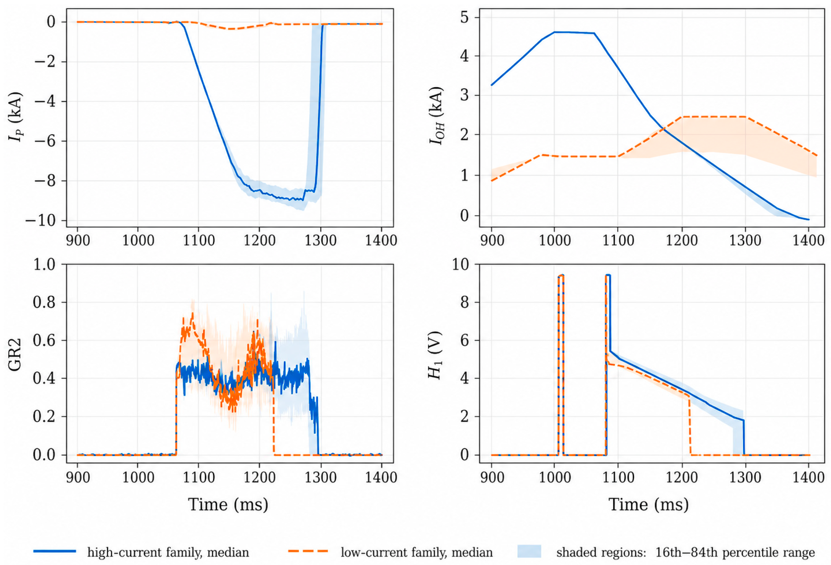
Figure 1 compares the typical waveforms of two groups of discharges. The high-current group contains discharges with max_t |I_p| > 5 kA, whereas the low-current group contains those with max_t |I_p| < 1 kA. For each signal and time sample, the figure shows the median over the discharges in the group. The shaded region extends from the 16th to the 84th percentile and therefore represents the variation between discharges.

The clearest difference between the two groups appeared in the OH coil waveform, which is consistent with its role as the main programmed drive of the plasma current. The ECRH and hydrogen signals show the additional operating conditions associated with each group, although their separation is less marked. The figure is intended to describe the dataset and the relation between the main inputs and the current amplitude, and it is not a model-performance figure.

The two current amplitude groups in Figure 1 are accompanied by clearly different OH coil programmes, so the observed separation does not by itself demonstrate two intrinsic plasma basins or a bifurcation. Within the selected dataset, OHI is the clearest operational separator, while ECRH, fuelling and wall-conditioning variables also covary with the scenarios. Because these inputs were not independently scanned, the present regression cannot assign causal responsibility for the separation to a single control knob. A dedicated classification or sensitivity study based on controlled actuator scans would be required to identify which programmed variables govern the transition between the observed amplitude families.

3. Symbolic Regression Methodology

3.1. Multigene Genetic Programming and Autoregressive Lag

Symbolic regression was used to obtain explicit algebraic estimators of the net plasma current waveform. Unlike a prescribed parametric regression, symbolic regression searches simultaneously over the structure of the equation and over its numerical coefficients. Candidate expressions are built from the selected input variables, constants and elementary functions and are selected according to training error and validation behaviour [9,10].

The model inputs and target are represented on a common 1 ms grid. During training, Δt defines the temporal spacing used to construct the regression examples. In the autoregressive models, it also defines the lag of the previous current input during both training and testing: the measured value I_p(t − Δt) is used during training, whereas the recursively predicted value Î_p(t − Δt) is used during testing. Non-autoregressive models use the actuator and conditioning variables but no previous measured or predicted value of I_p.

During recursive testing, the complete waveform is reconstructed on the original 1 ms grid. Thus, Δt determines the temporal spacing of the training pairs and, for autoregressive models, the feedback lag, but it does not set the spacing between consecutive test predictions. The MGGP search was repeated for Δt = 10, 5, 2 and 1 ms using the same train–validation–test split.

In MGGP, each candidate model is represented by a set of expression trees, or genes. Each gene defines a nonlinear function of the input vector, and the complete model is a linear combination of these nonlinear terms. For a non-autoregressive model:

$${\widehat{I}}_p\left(t\right)=a_0+{\displaystyle \sum _{j=1}^{N_g}}{a}_j{g}_j\left[\mathbf{x}\left(t\right)\right]$$

(2)

where g_j are evolved expression trees; a_j are linear coefficients fitted within the MGGP procedure; and N_g is the number of genes. Expression complexity is controlled by the maximum number of genes and the maximum tree depth.

For autoregressive symbolic models, the previous current state is added to the input vector:

$${\widehat{I}}_p\left(t\right)=a_0+{\displaystyle \sum _{j=1}^{N_g}}{a}_j{g}_j\left[\mathbf{x}\left(t\right),{\widehat{I}}_p\left(t-\Delta t\right)\right]$$

(3)

At test time, predictions are generated every 1 ms. For each discharge, the lagged current values required before a model prediction is available are initialized to zero. Thereafter, Î_p(t − Δt) is the prediction-generated Δt earlier. The equation therefore reconstructs the complete waveform without access to measured current values from the test discharge.

The main fitness measure is the root-mean-square error:

$$\mathrm{R}\mathrm{M}\mathrm{S}\mathrm{E}={\left[{\displaystyle \frac{1}{N}}{\displaystyle \sum _{i=1}^N}{\left(I_p\left(t_i\right)-{\widehat{I}}_p\left(t_i\right)\right)}^2\right]}^{1/2}$$

(4)

Model complexity is measured as the total number of nodes in the expression trees. This quantity has no direct physical meaning, but it is a useful measure of equation size and provides a practical indicator of interpretability and overfitting risk. In Equation (4), N is the number of evaluated samples used to calculate the RMSE for the corresponding dataset.

Each MGGP search begins with a random population of candidate equations. These equations are fitted to the training discharges and then modified through selection, crossover and mutation. The validation discharges are used to compare the candidate equations and retain the models and settings reported in this work. The test discharges are not used for model selection and are evaluated only after the equations have been fixed.

The symbolic searches used populations of approximately ${10}^3$ candidate equations. The unscaled autoregressive, general normalized and compact normalized models were evolved for 100, 50 and 70 generations, respectively. These settings correspond to the saved MGGP runs used in this study and were fixed from the training and validation workflow before the final test evaluation. Because MGGP is stochastic, the retained equations should be understood as selected representatives of their model classes rather than as unique symbolic optima. Repeated searches with predefined random seeds would be required to quantify variability due to the stochastic search procedure.

3.2. Model Classes, Autoregressive Memory and OH Amplitude Normalization

The symbolic analysis compares several model classes, each with a different amount of information available to the regression. MGGP determines the algebraic form of the equation within each class.

The simplest model is non-autoregressive: it estimates the plasma current without using any previous measured or predicted value of $I_p$:

$${\widehat{I}}_p\left(t\right)=f\left[\mathbf{x}\left(t\right)\right]$$

(5)

Here, x(t) contains the actuator and conditioning variables assigned to time t, including the OH coil current, its numerical time derivative, the heating and fuelling signals, the NBI actuators and the wall-conditioning variables. The derivative of the OH coil current contains local information about how that signal is changing and is calculated from neighbouring samples. The model is therefore not strictly memoryless. However, it does not receive the previous plasma current, a sequence of earlier inputs or an internal recurrent state.

This model is used as a baseline to determine how well the current can be estimated without explicit plasma current memory. The autoregressive models considered next additionally use the previous current value, allowing each prediction to depend directly on the preceding evolution of $I_p$. The second symbolic model class adds one lagged value of the plasma current. The current at time t is estimated from the actuator and conditioning variables at that time and from the current at t − $\Delta t$:

$${\widehat{I}}_p\left(t\right)=f\left[\mathbf{x}\left(t\right),{\widehat{I}}_p\left(t-\Delta t\right)\right]$$

(6)

This is called an autoregressive symbolic model because each prediction depends partly on the preceding current value. The previous current input gives the equation information about the recent evolution of the discharge that is not contained in the actuator values alone.

During MGGP training, the measured previous current is used with an artificial perturbation defined in Equation (7):

$${\widehat{I}}_p\left(t\right)=f\left[\mathbf{x}\left(t\right),{\tilde{I}}_p\left(t-\Delta t\right)\right],\hspace{1em}{\tilde{I}}_p\left(t-\Delta t\right)=I_p\left(t-\Delta t\right)+\eta \left(t-\Delta t\right)$$

(7)

Ref. [14] specifies a perturbation magnitude of 30% of the previous current value but does not specify its probability distribution. We therefore do not assign an undocumented distribution. The perturbation discourages the symbolic search from relying only on the measured previous current. During testing, the lagged current is initialized to zero, and subsequent predictions are fed back recursively. No measured plasma current value from a test discharge is used to initialize or update the prediction. Because predictions are reused as inputs, feedback errors can accumulate through the recursion [19]. The published equations do not contain the perturbation and require only the specified inputs and preprocessing. A systematic sensitivity study using different perturbation amplitudes was not performed. This training and testing mismatch is therefore treated as a limitation of the present recursive evaluation rather than as a controlled sensitivity result.

In this sense, the previous current input acts as a simple representation of the plasma state. It contains information about the recent current evolution, although it does not describe the current density profile or the full transport dynamics.

The third modification is applied only to the autoregressive symbolic models. Its purpose is to reduce the large difference in current amplitude between discharges before the MGGP search.

The regression error is expressed in kA. Consequently, a similar relative error produces a much larger absolute error in a high-current discharge than in a low-current one. Without normalization, the search may therefore focus mainly on the largest-current cases and give less importance to the shape of low-current waveforms.

To reduce this effect, each discharge is assigned one scale factor, S_oh, estimated from the maximum absolute OH-coil current in that discharge:

$$S_{\mathrm{O}\mathrm{H}}=2.303\underset{t}{\mathrm{m}\mathrm{a}\mathrm{x}}\left|I_{\mathrm{O}\mathrm{H}}\left(t\right)\right|-4.242 \mathrm{k}\mathrm{A}$$

(8)

where I_oh is expressed in kA. The coefficients were obtained from the training discharges and were then kept unchanged for validation and testing.

The whole plasma current waveform of each discharge is divided by this single value:

$$I_p^{\mathrm{s}\mathrm{c}}\left(t\right)={\displaystyle \frac{I_p\left(t\right)}{S_{\mathrm{O}\mathrm{H}}}}$$

(9)

MGGP is trained to predict the scaled waveform, Î_p^sc(t). The result is converted back to kA by multiplying it by the same factor:

$${\widehat{I}}_p\left(t\right)=S_{\mathrm{O}\mathrm{H}}\hspace{0.17em}{\widehat{I}}_p^{\mathrm{s}\mathrm{c}}\left(t\right)$$

(10)

The normalization therefore divides the prediction into two parts. The factor S_oh provides an approximate current amplitude for the discharge, while the symbolic equation predicts the evolution of the waveform after that amplitude difference has been reduced. The time-dependent OH signal may still appear inside the symbolic equation if MGGP selects it as an input.

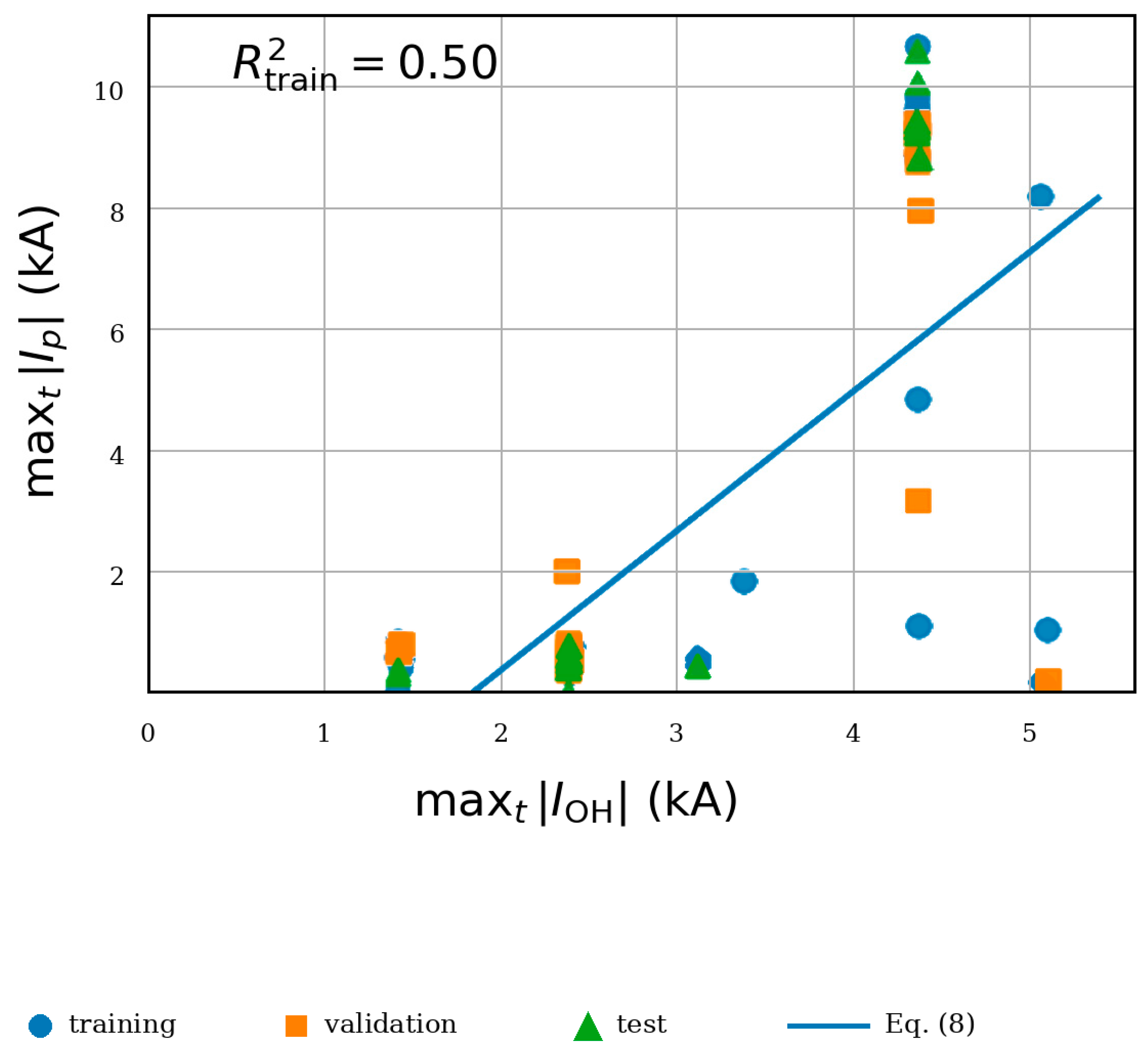
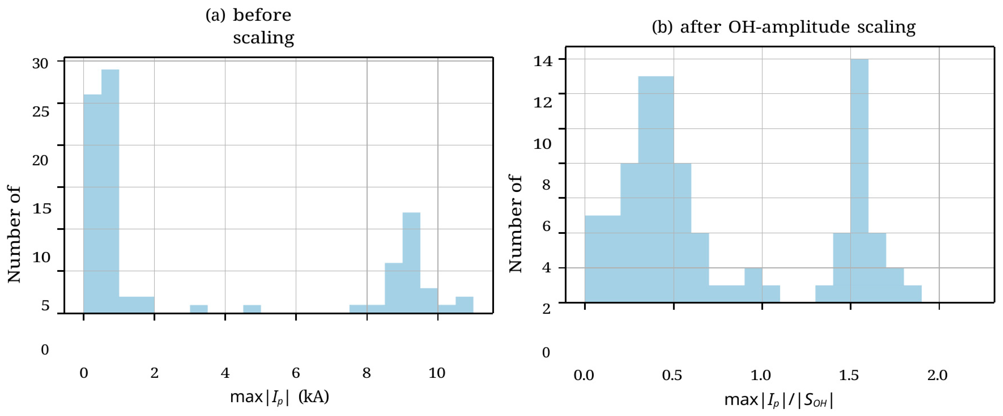
Figure 2 shows how the maximum plasma current amplitude varies with the maximum OH coil current. The points correspond to individual discharges, and the straight line is Equation (8). The relation has considerable scatter, with R² ≃ 0.50 on the training set. It is therefore not used as a physical model of current drive. Its only purpose is to provide an approximate amplitude scale for normalization. In Figure 3, we show the plasma current waveforms before and after this transformation. Before normalization, the high-current and low-current groups have clearly different amplitudes. After division by S_oh, this separation is considerably reduced. MGGP can then compare the waveform shapes of both groups on a more similar numerical scale.

The signed value of S_oh is used in Equations (9) and (10). The absolute value shown in the right panel of Figure 3 is used only to make the reduction in amplitude differences easier to visualize.

The normalization in Equation (8) was fitted using only the training discharges and evaluated only over the OH coil amplitude range represented in the dataset. The resulting symbolic equations are therefore restricted to this operating domain and should not be extrapolated to conditions for which the scale factor approaches zero. The 87 points represented in Figure 2 span approximately 1.42 ≤ max_t |I_oh| ≤ 5.10 kA. With Equation (8), this corresponds to a signed scale factor range of approximately −0.98 ≤ S_oh ≤ 7.51 kA. The scale would vanish at max_t |I_oh| ≃ 1.84 kA, but the smallest represented |S_oh| is about 0.93 kA, so none of the analysed discharges lie close to the singular point. Application near S_oh = 0 is nevertheless unsupported. The scatter visible in Figure 2 confirms that this factor is a numerical normalization, not a physical law for current drive. Alternative OH-based normalizations may be preferable for a broader operating range, but changing the normalization would define a different symbolic regression problem and would require a new model selection workflow.

The symbolic study therefore compares four cases: a non-autoregressive baseline, which estimates I_p(t) without a previous plasma-current value; an autoregressive model, which adds one previous current value; an OH-normalized autoregressive model, which also reduces the amplitude differences between discharges; and a compact normalized model, which retains the same autoregressive structure while restricting equation size.

4. Symbolic Regression Results

4.1. Symbolic Scans and Retained Equations

Table 1. Symbolic regression results for the equations retained using the training and validation discharges. The table reports their subsequent performance on the original 17-discharge test partition. Complexity is the total number of nodes in the symbolic expression.

Model	$\mathit{\Delta }\mathit{t}$ (ms)	Training RMSE (kA)	Test RMSE (kA)	Complexity
Without previous current input	1	0.8983	1.2955	–
With previous current input	10	0.2663	0.6557	148
With previous current input and OH normalization	5	0.0907	0.4898	98
Compact model with previous current input and OH normalization	10	0.1097	0.5700	36

compares four versions of the symbolic model in the original symbolic regression study. The first estimates the plasma current without using any previous value of $I_p$. The second also receives the current value at the autoregressive lag $\Delta t$. The third adds the OH amplitude normalization described above. The fourth uses the same lagged-current input and normalization but restricts the size of the resulting equation.

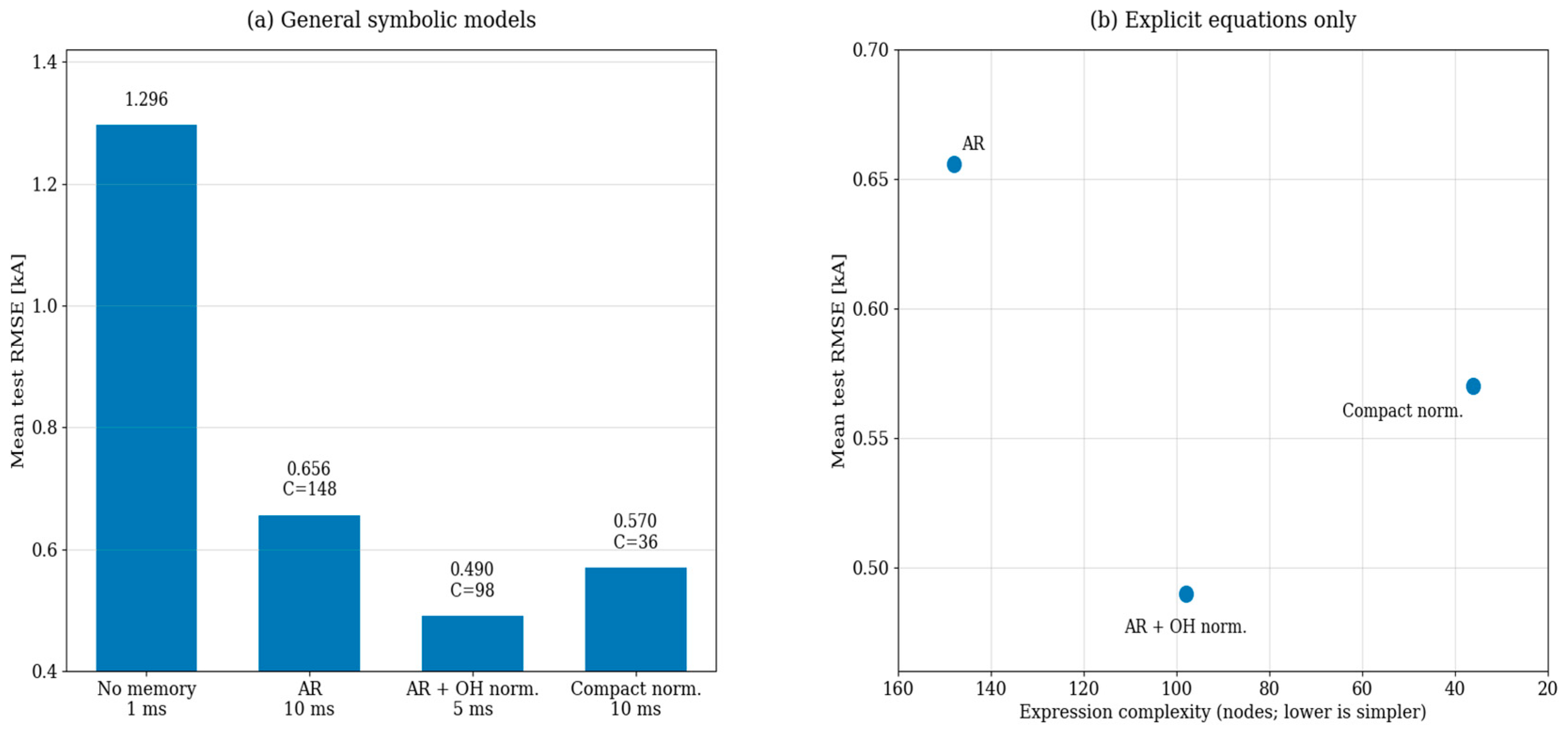
For each model family and value of $\Delta t$, the retained equation was selected using the training and validation discharges. Table 1 reports the training RMSE and the subsequent RMSE obtained on the original 17-discharge test partition. The model without previous current information had a test RMSE of 1.2955 kA, the autoregressive model was 0.6557 kA, and the OH-normalized autoregressive model was 0.4898 kA. The compact normalized equation was 0.5700 kA while reducing the expression size from 98 to 36 nodes. Since the training time step, the autoregressive lag, equation structure and MGGP run differ between rows, the numerical changes should not be interpreted as the effect of only one modification. The final comparison between the selected symbolic equations and the NARX-RNN is based on the 15-discharge valid signal set in Section 6.

Table 2. Symbolic regression results without previous current input or OH amplitude normalization. The retained equations were selected using validation data, and the table reports their training and test RMSE values.

$\mathit{\Delta }\mathit{t}$ (ms)	Training RMSE (kA)	Test RMSE (kA)
10	0.8298	1.3372
5	0.8769	1.3098
2	0.9035	1.3230
1	0.8983	1.2955

and

Table 3. Symbolic regression results with previous current input, without and with OH amplitude normalization. The retained equations were selected using validation data, and the table reports their training and test RMSE values in kA.

$\mathit{\Delta }\mathit{t}$ (ms)	AR Train	AR test	AR + OH Train	AR + OH Test	Complexity
10	0.2663	0.6557	0.0925	0.5572	138
5	0.2837	1.0582	0.0907	0.4898	98
2	0.2233	0.9957	0.0816	2.6907	135
1	0.2054	2.2810	0.0668	2.7420	99

show the results obtained for $\Delta t$ = 1, 2, 5 and 10 ms. In the non-autoregressive models, $\Delta t$ specifies the temporal spacing used to construct the training pairs. In the autoregressive models, it also specifies the feedback lag during recursive prediction. All test waveforms are reconstructed on the 1 ms grid.

Because the rows differ in autoregressive lag, normalization and expression restrictions, Table 1 is intended as a comparison of retained model classes, not as a formal one variable sensitivity analysis or exhaustive hyperparameter optimization.

For the model without previous current information, changing the temporal spacing used to construct the training pairs has only a small effect on the test error. This indicates that temporal subsampling during training does not compensate for the absence of information about the preceding plasma current.

The models that use the previous current are more sensitive to $\Delta t$. Among the reported test results, the lowest error without OH normalization occurred for an autoregressive lag of 10 ms, while the lowest error after normalization occurred for a lag of 5 ms. The errors increased markedly for lags of 2 and 1 ms. A possible explanation is that shorter lags reintroduce each prediction error into the model after fewer milliseconds, allowing it to propagate through a larger number of feedback iterations over the same discharge interval. Since MGGP starts from a random population of equations, repeated runs would be required to determine whether this behaviour is systematic. The equations and their settings were selected using the training and validation discharges; the test values are reported only as their final evaluation.

Figure 4 separates the full search-level comparison from the equation-level comparison. Panel (b) includes the unnormalized autoregressive run as a complexity reference together with the two OH-normalized equations. Only the latter two are available as complete expressions and are analysed algebraically below. Among the equations retained using the validation data, the general normalized equation gave the lowest test RMSE, whereas the compact equation reduced the node count from 98 to 36. The compact equation was retained as a low-complexity reference that can be inspected and implemented directly.

For two representative MGGP runs, the held-out validation RMSE is reported explicitly. For the unnormalized autoregressive model with Δt = 10 ms, the training and validation RMSE values were 0.2663 and 0.2615 kA, respectively. For the OH-normalized autoregressive run with Δt = 10 ms, the corresponding values were 0.0925 and 0.1221 kA [14]. These values document validation behaviour during the original model development workflow. The test values in Table 1, Table 2, Table 3 and

Table 4. Low-complexity symbolic regression runs. MG is the maximum number of genes and TD the maximum tree depth. Candidate equations were retained using validation performance; the table reports their final test RMSE values. The italicized row corresponds to the compact equation analysed in the text.

$\mathit{\Delta }\mathit{t}$ (ms)	Restriction	Test RMSE (kA)	Complexity
10	$MG=5$, $TD=3$	0.7273	67
5	$MG=5$, $TD=3$	0.5637	59
10	$MG=4$, $TD=3$	0.7687	54
5	$MG=4$, $TD=3$	0.7710	59
10	$MG=3$,$TD=3$	0.5700	36
5	$MG=3$, $TD=3$	0.7064	39

are post-selection evaluations and were not used as model selection criteria.

4.2. Selected OH-Normalized Symbolic Models

The detailed discussion focuses on two complete OH-normalized autoregressive equations retained using the validation discharges. The general equation was selected for its validation performance, whereas the compact equation was retained because it provides a shorter expression with competitive validation accuracy. Their test results are presented only as the final evaluation of the already selected equations.

Both equations were retained in the original validation guided workflow, and their test results are presented only as post selection evaluations.

The general symbolic equation uses an autoregressive lag of Δt = 5 ms. Because the model was fitted to the scaled current defined in Equation (9), the equation is written for Î_p^sc(t). The current in physical units is recovered afterwards using Î_p(t) = S_oh Î_p^sc(t), as defined in Equation (10). With rounded coefficients, the equation is:

$$\begin{gathered} {\widehat{I}}_p^{\mathrm{s}\mathrm{c}}\left(t\right)=-0.05415\mathrm{G}\mathrm{R}2-0.01755{\widehat{I}}_p^{\mathrm{s}\mathrm{c}}{\left(t-\Delta t\right)}^2+0.05415H{\widehat{I}}_p^{\mathrm{s}\mathrm{c}}\left(t-\Delta t\right) \\ +0.2212BH{\widehat{I}}_p^{\mathrm{s}\mathrm{c}}\left(t-\Delta t\right)-0.003B{\widehat{I}}_p^{\mathrm{s}\mathrm{c}}{\left(t-\Delta t\right)}^3 \\ +0.01769I_{\mathrm{O}\mathrm{H}}\left[{\widehat{I}}_p^{\mathrm{s}\mathrm{c}}\left(t-\Delta t\right)-H{\widehat{I}}_p^{\mathrm{s}\mathrm{c}}\left(t-\Delta t\right)\right] \\ -0.01919BH{\widehat{I}}_p^{\mathrm{s}\mathrm{c}}\left(t-\Delta t\right)\left[H-{\widehat{I}}_p^{\mathrm{s}\mathrm{c}}\left(t-\Delta t\right)\right]-5.002\times {10}^{-5} \end{gathered}$$

(11)

Here, H is the hydrogen valve signal, B is the normalized boronization counter and S_oh is the discharge-level normalization factor obtained from the OH programme.

The equation combines the previous scaled-current estimate with the present values of the OH coil current, ECRH, hydrogen fuelling and wall-conditioning state. The terms containing powers of Î_p^sc(t − Δt) allow the current evolution to depend nonlinearly on its preceding value. The products involving H and B indicate that the contribution of this previous current information changes with fuelling and wall conditions. The OH coil current also enters explicitly, in addition to its role in the normalization factor S_oh. No NBI variable appears in this retained equation, although the NBI acceleration current and acceleration voltage signals were available to the MGGP search. These terms describe the combinations of variables selected by MGGP because they improve prediction. They should not be interpreted individually as transport laws or as direct causal relations. The equation is an empirical estimator for the operating range represented by the dataset.

4.3. Compact Symbolic Model

The compact model is a low-complexity member of the OH-normalized autoregressive family. It was obtained by limiting the maximum number of genes and the maximum tree depth. It estimates the scaled current Î_p^sc(t):

$$\begin{gathered} {\widehat{I}}_p^{\mathrm{s}\mathrm{c}}\left(t\right)=-0.009643+0.2754\sqrt{\mathrm{G}\mathrm{R}2}{\widehat{I}}_p^{\mathrm{s}\mathrm{c}}\left(t-\Delta t\right)+0.01653{\displaystyle \frac{H{\widehat{I}}_p^{\mathrm{s}\mathrm{c}}\left(t-\Delta t\right)}{\mathrm{L}\mathrm{i}}} \\ +0.00915\mathrm{G}\mathrm{R}2H{\widehat{I}}_p^{\mathrm{s}\mathrm{c}}{\left(t-\Delta t\right)}^2 \end{gathered}$$

(12)

with an autoregressive lag of Δt = 10 ms.

The expression contains a constant offset, an ECRH-conditioned memory term, a hydrogen–wall-state memory term and a nonlinear ECRH–fuelling–memory term.

The compact equation does not contain an explicit term in the instantaneous OH coil current. Its main dependence on the OH programme enters through the normalization factor S_oh. The symbolic equation predicts the scaled current Î_p^sc(t), and the current in physical units is recovered as:

$${\widehat{I}}_p\left(t\right)=S_{\mathrm{O}\mathrm{H}}{\widehat{I}}_p^{\mathrm{s}\mathrm{c}}\left(t\right)$$

(13)

Thus, S_oh provides the approximate current scale of the discharge, while the compact equation describes the time evolution of the normalized current using ECRH, hydrogen fuelling, wall conditioning and the previous scaled-current value.

The absence of a free additive OH term in the compact equation does not imply that the OH programme is absent from the model. Its main OH dependence is carried by the discharge-level normalization factor, while the recursive expression describes the evolution of the normalized current. The compact equation is therefore useful as a short, directly inspectable current-response map despite its lower average accuracy.

Table 4 shows the low-complexity search associated with Equation (12). The candidate equations were compared using the validation discharges. The reported MG = 3, TD = 3 equation with an autoregressive lag of Δt = 10 ms was retained because it provides a particularly short complete expression with satisfactory validation performance. The test RMSE values in the table are presented only to report the final performance of the retained equations.

4.4. Interpretation and Limits of the Symbolic Equations

The selected symbolic equations provide empirical current response maps for the selected TJ-II operating domain. Their common structure separates a discharge-level OH-related amplitude factor from a normalized recursive response involving previous current, heating, fuelling and wall-conditioning variables. This structure is consistent with TJ-II OH-programmed experiments in which OH programming modifies the net plasma current and the rotational transform profile [2]. In the present models, however, S_oh is used only as an amplitude normalization fitted on the training set.

The symbolic results indicate that previous current information is important. Models using actuator values without a previous current input do not reconstruct the waveform as accurately as the best autoregressive runs. Including the previous scaled-current state Î_p^sc(t − Δt) provides information about recent plasma evolution that is not contained in the present actuator values alone.

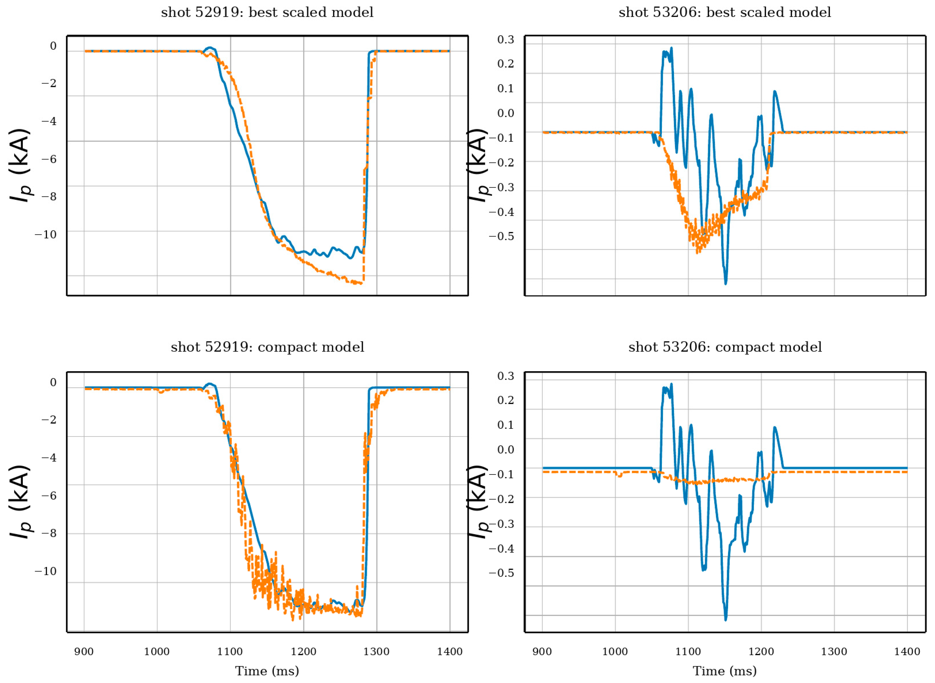
Figure 5 compares the two selected symbolic equations for one high-current and one low-current test discharge. Discharge 52919 represents the high-current group, while discharge 53206 represents the low-current group. These examples illustrate the behaviour of the equations in two different current ranges; the quantitative comparison between models is based on the 15-discharge valid signal test set and is presented later.

For discharge 52919, both equations reproduce the main decrease, the negative current phase and the final recovery. The general equation follows the measured waveform more smoothly, although it predicts a somewhat larger current magnitude near the end of the negative current phase. The compact equation captures the overall evolution but produces larger short-time variations.

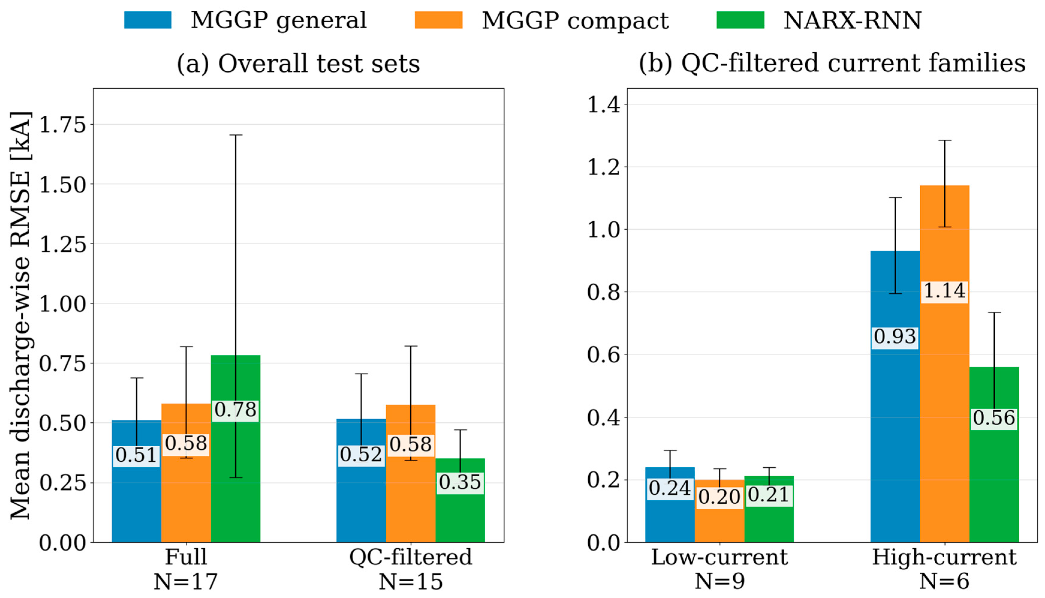
The low-current case is more difficult. For discharge 53206, the measured current contains several rapid oscillations of both signs. The general equation reproduces the broad negative trend but not the individual oscillations. The compact equation gives an almost constant, slightly negative estimate and does not reproduce the measured waveform. This difference shows that an equation may describe the main evolution of large-current discharges while losing important details when the current amplitude is small. Two distinct effects may contribute to this behaviour. First, when the current amplitude is small, a given absolute measurement or baseline uncertainty represents a larger fraction of the signal. Second, some rapid fluctuations may reflect plasma dynamics that are not encoded in the selected actuator and conditioning inputs: for example, dynamics associated with density, radiation or MHD activity. The present data do not allow these contributions to be separated quantitatively. The corresponding current-regime comparison is presented later in Section 6. In the low-current group, the mean discharge wise RMSE values are approximately 0.24, 0.20 and 0.21 kA for the general MGGP, compact MGGP and NARX-RNN models, respectively. In the high-current group, the corresponding values are approximately 0.93, 1.14 and 0.56 kA. Thus, the three models are comparable in the low current group, whereas the NARX-RNN gives the lowest observed mean RMSE in the high current group.

5. Recurrent Neural Network Model

5.1. NARX-RNN Formulation

The neural estimator has the same purpose as the autoregressive symbolic models: to estimate the plasma current waveform from the programmed signals and from the recent evolution of the current. Both approaches can represent nonlinear relations. The main difference is how those relations are expressed. MGGP produces an explicit mathematical equation that can be written and inspected term by term. The neural model instead represents the relation through many fitted internal parameters, so its prediction cannot be reduced to a single explicit equation.

The model is a nonlinear autoregressive recurrent neural network with exogenous inputs (NARX-RNN). Here, “autoregressive” means that the prediction uses previous values of the plasma current, while “exogenous inputs” refers to the actuator and wall-conditioning signals supplied to the model. The recurrent part of the network is built with long short-term memory (LSTM) layers, which allow the model to use information from several previous time samples [20,21].

At each step, the network predicts the current at the next sample from two groups of inputs:

$${\widehat{I}}_{p,k+1}=F_{\theta }\left({\mathbf{u}}_{k-9:k},{\mathbf{h}}_k\right)$$

(14)

where the trained neural network is denoted by F_θ.

The first input, u_k−9:k, contains the sequence of exogenous operational signals over the ten most recent samples, from k 9 to k. At each time step, the corresponding exogenous input vector is defined as:

$${\mathbf{u}}_k={\left[I_{\mathrm{O}\mathrm{H},k},{\mathrm{G}\mathrm{R}2}_k,H_k,{\mathrm{L}\mathrm{i}}_k\right]}^T$$

(15)

where I_OH,k is the OH coil current, GR2_k is the ECRH gyrotron signal, H_k is the hydrogen fuelling signal, and Li_k is the lithium wall-conditioning counter. Thus, the exogenous branch receives the recent evolution of externally programmed or operationally prescribed quantities without using the measured plasma current from the test discharge.

The second input contains the nine most recent plasma current values:

$${\mathbf{h}}_k={\left[I_{p,k-8},I_{p,k-7},\dots ,I_{p,k}\right]}^T$$

(16)

The use of several previous samples distinguishes the neural model from the symbolic equations considered above, which use only one previous current value. The network can therefore combine a longer recent history of both the actuator signals and the plasma current.

For the NARX-RNN, training and validation use measured current history, whereas testing starts from a zero-current history and subsequently uses only recursively predicted values. The exogenous input window is always formed from the available operational signals. This difference between training and testing can lead to error accumulation. No measured plasma current value from a test discharge is used to initialize or update the prediction, and a dedicated sensitivity study of recursive feedback was not performed. The recursive test therefore evaluates the network using its own previous current predictions.

The final architecture was fixed before the independent test evaluation. Its hyperparameters were selected from a small set of nearby configurations using the validation data, with the aim of obtaining a compact model suitable for recursive prediction. The nine-sample current history window was chosen as a compromise between providing short term memory and limiting the accumulation of feedback errors. The model contains two recurrent branches. The exogenous branch receives the 10-sample sequence of programmed inputs from k-9 to k and uses an LSTM layer with 128 units. The current history branch receives the nine previous current values and uses a smaller LSTM layer with 16 units. Each branch is followed by layer normalization, which stabilizes the internal activations during training [22]. The two outputs are concatenated and passed through dense layers with 32 and 16 units before a linear output layer. The model is trained with mean-square-error loss and the Adam optimizer [23]. A targeted validation set sweep was performed over nearby configurations, including smaller and larger recurrent layers and nearby history lengths. Among the configurations explored, the retained architecture gave the best validation performance and was therefore fixed before the independent test evaluation. This search was intended to select a compact recurrent estimator suitable for recursive prediction rather than to perform an exhaustive optimization of the neural architecture.

All input variables and the target plasma current are standardized using scalers fitted on the training set only. This transformation is used solely as a numerical preprocessing step to improve neural network training and is then inverted when reporting predictions in physical units. It should not be confused with the OH amplitude normalization used in the symbolic regression equations, where the fitted factor $S_{\mathrm{O}\mathrm{H}}$ is part of the explicit predictive model itself.

The four-input architecture and its layer sizes were selected in the original training and validation workflow. The independent test set was not used for this selection. The reported result corresponds to one final trained instance, while the absence of a systematic analysis with repeated random seeds is discussed in Appendix A.

5.2. Recursive Test

The neural network was tested on the same 17 discharges used in the symbolic regression analysis.

All models were compared over the same time window and the same time samples.

During the test, the network is not given the measured plasma current of the discharge under evaluation. At the beginning of each test discharge, the nine previous current entries are set to zero. The network then predicts the next value of $I_p$. This predicted value is inserted into the current history buffer and used as an input for the following time step. The process is repeated until the complete waveform is reconstructed. In this way, the test evaluates whether the model can reconstruct the current waveform from the operational input signals and from its own previous predictions. Measured current samples from the test discharge are never used to start or advance the recursive prediction.

Following the routine signal quality control described in Section 2.1, the final quantitative analysis used 15 test discharges. No model was retrained or modified as a result of this review.

5.3. Neural Network Performance on the Test Set

Table 5. NARX-RNN errors on the 15-discharge valid signal test set retained after signal quality control.

Set	$\mathit{N}$	Mean MAE (kA)	Mean RMSE (kA)	Median RMSE (kA)
Valid signal test set	15	0.2862	0.3501	0.2304

summarizes the NARX-RNN performance on the 15 test discharges with valid OHI and plasma current signals. The mean discharge-wise RMSE is 0.350 kA, and the median is 0.230 kA. The corresponding mean MAE is 0.286 kA.

The mean absolute error (MAE) is the average absolute difference between the measured and predicted current. The RMSE gives more weight to large deviations and is used as the main comparison metric.

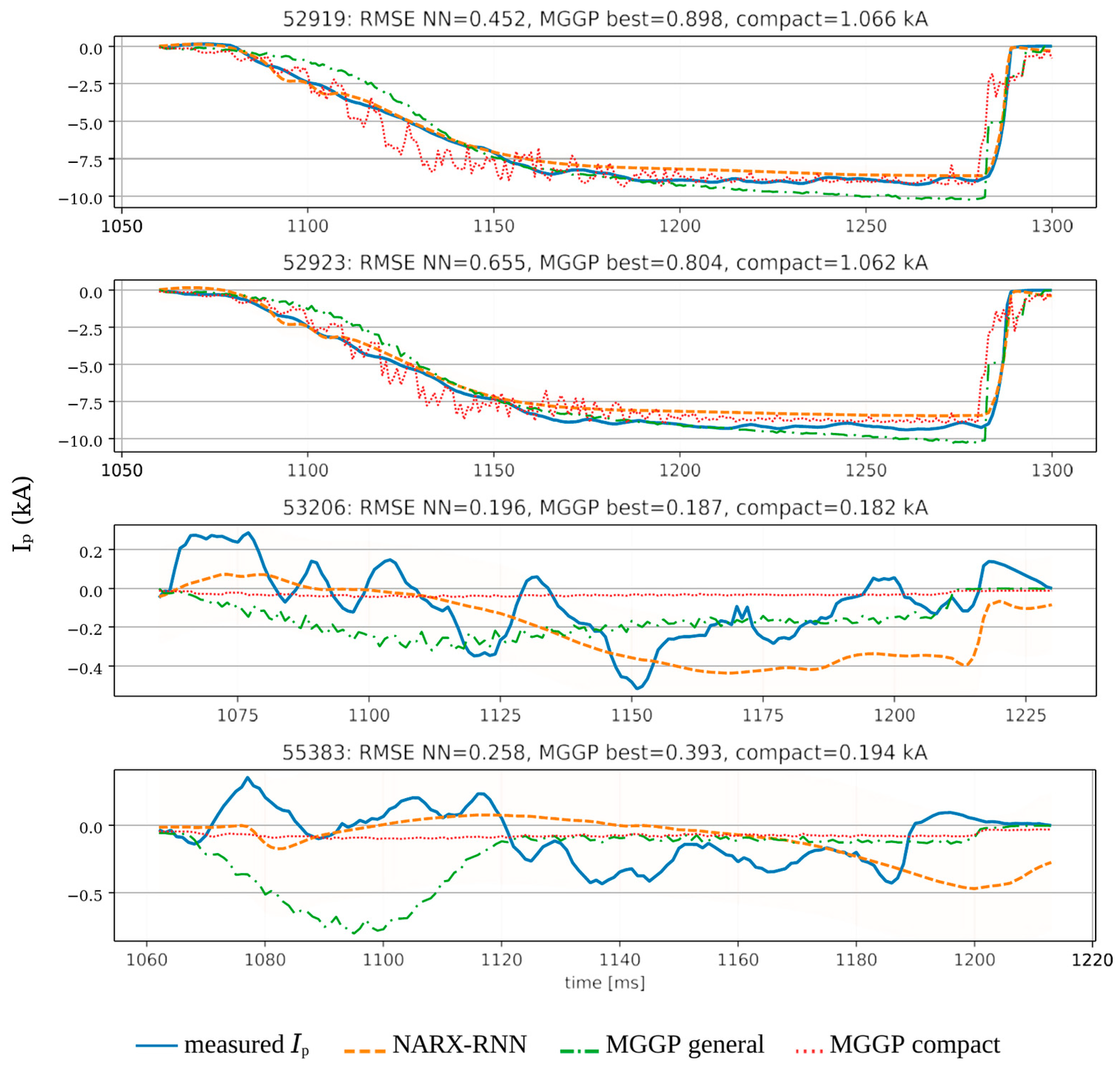
Figure 6 compares the NARX-RNN with the general and compact symbolic equations for four test discharges with complete, non-zero target signals. Two examples belong to the high-current group and two to the low-current group. These waveforms illustrate the behaviour of the models, while the numerical comparison below uses all 15 discharges in the valid signal test set.

In the high-current examples, the NARX-RNN follows the measured waveform more closely than the symbolic equations. This is consistent with the fact that the neural model uses ten recent samples of the actuator signals and nine recent current values, whereas the symbolic equations use only one previous current value. In the low-current examples, the differences between the three models are smaller, although none of them reproduced every rapid variation of the measured signal.

6. Comparison of the Symbolic and Neural Models

Comparison on the same discharges. The three estimators were compared using the same time samples from the 15 test discharges retained after signal quality control.

On this common set, the NARX-RNN gave the lowest mean RMSE, 0.350 kA, followed by the general symbolic equation with 0.515 kA and the compact symbolic equation with 0.576 kA. The corresponding median values were 0.230, 0.301 and 0.252 kA, respectively.

The lower mean error of the NARX-RNN indicates that it reproduced the valid test waveforms more accurately on average. The compact symbolic equation has a median error close to that of the neural model, while providing a much shorter and fully explicit mathematical expression.

Here, “transparent” refers to the mathematical representation of the estimator, not to causal physical interpretation. The MGGP models yield explicit closed form expressions, Equations (11) and (12), so the variables, nonlinear combinations and numerical coefficients used to produce a prediction can be inspected directly, and the equations can be evaluated independently of the training software. By contrast, the NARX-RNN input output relation is distributed over many learned weights and recurrent hidden states, and no single comparable closed form equation can be extracted from the trained network. This is the sense in which the symbolic estimator is more transparent. It does not imply that individual MGGP terms are transport laws or causal mechanisms. “Direct implementation” similarly means that the published algebraic expression can be evaluated from the specified inputs and preprocessing constants without loading the trained neural network model. Once training is complete, inference with both approaches is computationally inexpensive for the present application, so computational cost is not claimed as a decisive advantage of MGGP.

To place these errors in a physical context, net current variations of a few kA can produce appreciable changes in the edge rotational transform profile in TJ-II [1,2]. Within the linear approximation of Equation (1), current errors of 0.25, 0.5 and 1 kA correspond to local rotational transform uncertainties of 0.25C(ρ), 0.5C(ρ) and 1.0C(ρ), respectively, with C expressed per kA. The associated radial displacement of a rational surface is δρ_r ≃ −C(ρ_r)δI_p/[(∂ι/∂ρ) at ρ = ρ_r]. Consequently, the same current error can imply different radial displacements for different rational surfaces and local magnetic shear. The RMSE values are therefore reported primarily as current prediction errors. No universal 0.25 kA threshold or superiority over simpler linear or physics-based baselines is claimed.

The valid signal test set contained only 15 discharges, so the mean RMSE may depend noticeably on the particular discharges included. A paired nonparametric bootstrap was therefore applied over discharge indices. For each resample, 15 discharge indices were drawn with replacement, and the same sampled indices were used for all three estimators. The mean RMSE was recalculated for every resample, and the central 95% of the resulting values is reported in

Table 6. Discharge-wise RMSE on the 15-discharge valid signal test set. Brackets show the bootstrap 95% interval for the mean RMSE.

Model	$\mathit{N}$	Mean RMSE (kA)	Median (kA)	Maximum (kA)
MGGP general	15	0.515 [0.336, 0.706]	0.301	1.298
MGGP compact	15	0.576 [0.343, 0.822]	0.252	1.435
NARX-RNN	15	0.350 [0.247, 0.471]	0.230	0.846

and Figure 7 [24]. The resampling is paired because every bootstrap replicate uses the same discharge indices for all three estimators. The brackets reported in Table 6 are nevertheless marginal confidence intervals for each model’s mean RMSE, not confidence intervals for pairwise differences and not hypothesis test p values. These intervals describe the uncertainty associated with the limited number of valid test discharges. They do not represent uncertainty in the Rogowski coil measurement, uncertainty in the fitted model parameters or a prediction interval for a new discharge. Since the intervals partially overlap and training stochasticity is not included, we do not claim statistical significance for the differences between model classes. The result is interpreted as the observed performance ordering for this fixed dataset and these retained models, not as a general proof that one model class will dominate after retraining or under other operating conditions.

Figure 7a contrasts the mean discharge-wise RMSE on the original 17-discharge test partition with that of the 15-discharge valid signal set. Error bars show bootstrap intervals for each displayed set; the valid signal intervals are also reported in Table 6. Panel (b) reports the valid discharges that satisfy the high- and low-current thresholds defined in Section 2; valid discharges outside both thresholds are not included in that panel. The NARX-RNN has the lowest observed mean RMSE in the high-current group, whereas the three methods give errors of comparable magnitude in the low-current group.

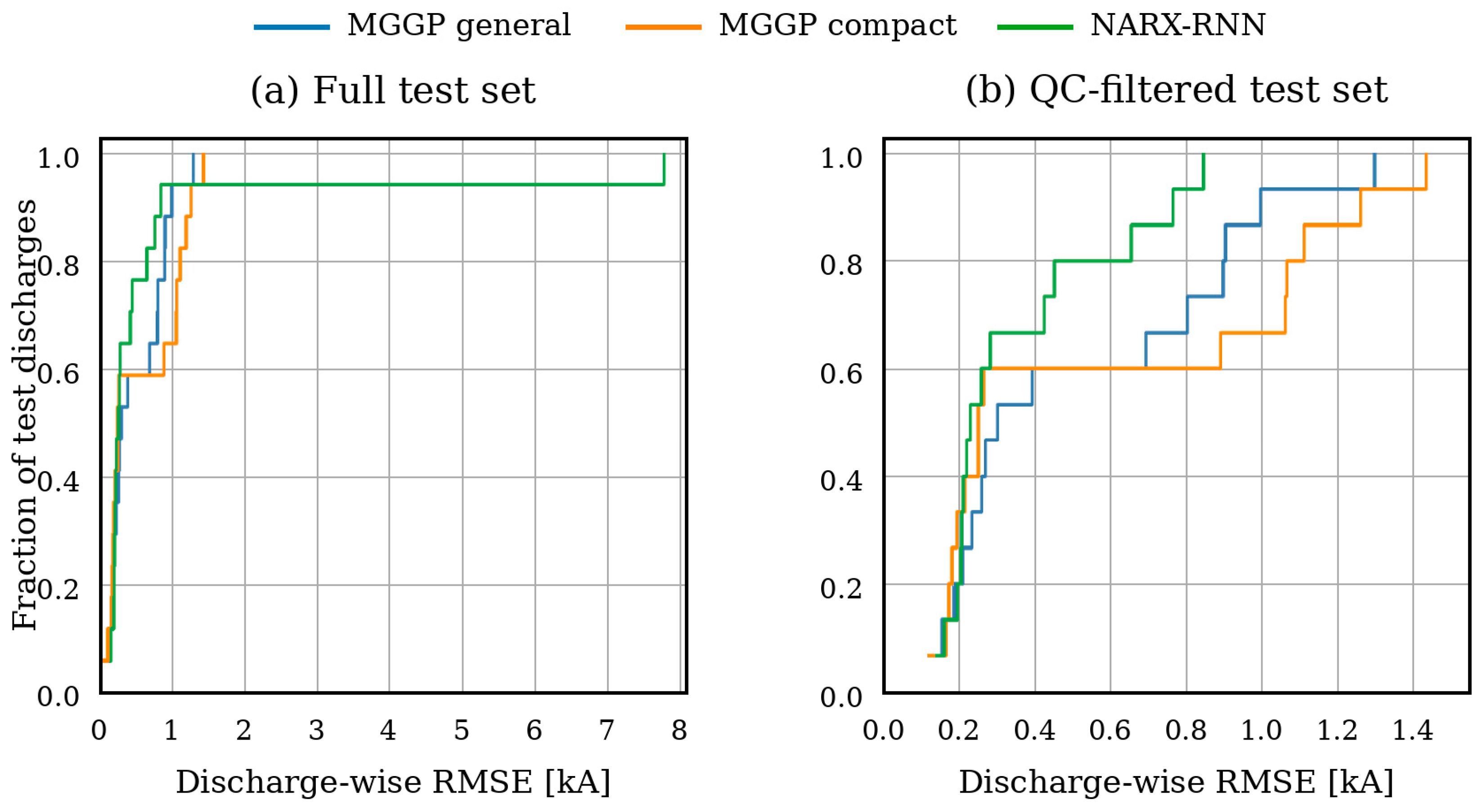
Figure 8 presents the discharge-wise errors in cumulative form for both the original 17-discharge partition and the 15-discharge valid signal set. For any RMSE value on the horizontal axis, the vertical axis gives the fraction of discharges with an error below that value. A curve located further to the left therefore indicates lower errors for a larger fraction of the test set. The final comparison is based on the valid signal set shown in panel (b), where the NARX-RNN curve is generally shifted towards lower RMSE values, in agreement with its lower mean and median errors.

7. Conclusions

This study compared explicit MGGP equations and a NARX-RNN for estimating net plasma current waveforms in 87 OH-programmed TJ-II discharges from the magnetic configuration 100_44_64. On the original test partition, the retained non-autoregressive symbolic model gave an overall RMSE of 1.296 kA, whereas the OH-normalized autoregressive equation gave 0.490 kA. A compact 36-node equation achieved 0.570 kA, providing a shorter expression that can be inspected and implemented directly.

On the 15-discharge set used for the final comparison, the NARX-RNN gave the lowest mean and median discharge-wise RMSE: 0.350 and 0.230 kA, respectively. The corresponding values were 0.515 and 0.301 kA for the general symbolic equation and 0.576 and 0.252 kA for the compact equation. Whether these current error levels are sufficient for positioning a particular rational surface must be assessed for the selected surface and magnetic configuration using the local rotational transform response and magnetic shear. No universal 0.25 kA control threshold is inferred from the present data. Because the retained estimators differ in input set and temporal information, the reported errors should be interpreted as the performance of these specific models on the present dataset, not as a general ranking of MGGP and NARX-RNN.

The symbolic equations are empirical estimators and remain restricted to the operating range and preprocessing used in this study. The reported results apply to TJ-II configuration 100_44_64 and to the operating range represented in this dataset. Generalization to other magnetic configurations or operating regimes has not been demonstrated and would require dedicated validation with additional discharges. Future work should include repeated training with predefined random seeds, comparisons using identical inputs, simple ARX or state space baselines, and additional magnetic configurations. Future applications will use these predictions for OH programming and rotational transform control in TJ-II.

References

1. López-Bruna, D.; Castejón, F.; Estrada, T.; Romero, J.A.; Jiménez, J.A.; Ascasíbar, E.; the TJ-II Team. Effects of ohmic current in the TJ-II stellarator. Nucl. Fusion 2004, 44, 645–654. [Google Scholar] [CrossRef] [Scilit]
2. van Milligen, B.; García-Cortés, I.; McCarthy, K.J.; Carreras, B.A.; García, L.; Cappa, Á.; Pons-Villalonga, P.; Estrada, T.; Medina-Roque, D.; Hernández-Sánchez, J. The rotational transform and enhanced confinement in the TJ-II stellarator. J. Plasma Phys. 2025, 91, E98. [Google Scholar] [CrossRef] [Scilit]
3. van Milligen, B.; Estrada, T.; Carreras, B.A.; García, L.; the TJ-II Team. Importance of the rotational transform for L–H transitions in the TJ-II stellarator. Plasma 2024, 7, 446–464. [Google Scholar] [CrossRef] [Scilit]
4. Panadero, N.; McCarthy, K.J.; Pégourié, B.; Carrasco, R.; García-Cortés, I.; García, R.; Hernández-Sánchez, J.; Köchl, F.; Martínez-Fernández, J.; Sakamoto, R.; et al. Using rational surfaces to improve pellet fuelling in stellarators. J. Plasma Phys. 2023, 89, 955890601. [Google Scholar] [CrossRef] [Scilit]
5. Rattá, G.A.; Vega, J.; Murari, A.; Vagliasindi, G.; Johnson, M.F.; de Vries, P.C.; JET EFDA Contributors. An advanced disruption predictor for JET tested in a simulated real-time environment. Nucl. Fusion 2010, 50, 025005. [Google Scholar] [CrossRef] [Scilit]
6. Rattá, G.A.; Vega, J.; Murari, A.; JET EFDA Contributors. Simulation and real-time replacement of missing plasma signals for disruption prediction: An implementation with APODIS. Plasma Phys. Control. Fusion 2014, 56, 114004. [Google Scholar] [CrossRef] [Scilit]
7. Velasco, J.L.; Allmaier, K.; López-Fraguas, A.; Beidler, C.D.; Maassberg, H.; Kernbichler, W.; Castejón, F.; Jiménez, J.A. Calculation of the bootstrap current profile for the TJ-II stellarator. Plasma Phys. Control. Fusion 2011, 53, 115014. [Google Scholar] [CrossRef] [Scilit]
8. Mulas, S.; Cappa, A.; Martínez-Fernández, J.; Bruna, D.L.; Velasco, J.L.; Estrada, T.; Gómez-Manchón, J.M.; Liniers, M.; McCarthy, K.J.; Pastor, I.; et al. Validating neutral-beam current drive simulations in the TJ-II stellarator. Nucl. Fusion 2023, 63, 066026. [Google Scholar] [CrossRef] [Scilit]
9. Koza, J.R. Genetic Programming: On the Programming of Computers by Means of Natural Selection; MIT Press: Cambridge, MA, USA, 1992. [Google Scholar]
10. Searson, D.P. GPTIPS 2: An open-source software platform for symbolic data mining. arXiv 2014, arXiv:1412.4690. [Google Scholar]
11. Schmidt, M.; Lipson, H. Distilling free-form natural laws from experimental data. Science 2009, 324, 81–85. [Google Scholar] [CrossRef] [Scilit] [PubMed]
12. Brunton, S.L.; Proctor, J.L.; Kutz, J.N. Discovering governing equations from data by sparse identification of nonlinear dynamical systems. Proc. Natl. Acad. Sci. USA 2016, 113, 3932–3937. [Google Scholar] [CrossRef] [Scilit] [PubMed]
13. González-Ganzábal, A.; Rattá, G.A.; Estrada, T.; Martínez-Fernández, J.; Panadero, N.; Cappa, Á.; López-Miranda, B.; Baciero, A.; Martín, F.; Tafalla, D.; et al. A comprehensive database of TJ-II signals and diagnostics for statistically based models. Fusion Eng. Des. 2026, 224, 115613. [Google Scholar] [CrossRef] [Scilit]
14. Blas, V.A.F. Estimación de Señales del Plasma Mediante Técnicas de Inteligencia Artificial. Master’s Thesis, Universidad Autónoma de Madrid, Madrid, Spain, 2025. [Google Scholar]
15. Romero, J.A.; Pacios, L.; de la Peña, A.; Lapayese, F.; Ascasíbar, E. Magnetic configuration sweep control in heliac type stellarators. Nucl. Fusion 2014, 54, 043008. [Google Scholar] [CrossRef] [Scilit]
16. Martínez-Fernández, J.; Cappa, Á.; Tereshchenko, M.; Tolkachev, A.; Ros, A.; Catalán, G. High power characterisation of the ECRH transmission lines and power deposition calculations in the TJ-II stellarator. Fusion Eng. Des. 2020, 161, 112065. [Google Scholar] [CrossRef] [Scilit]
17. Pacios, L.; Labrador, I.; de la Peña, A.; Carrasco, R.; Lapayese, F. Gas inlet control system for the stellarator TJ-II. In Proceedings of the 1999 IEEE Conference on Real-Time Computer Applications in Nuclear Particle and Plasma Physics. 11th IEEE NPSS Real Time Conference. Conference. Conference Record (Cat. No.99EX295); IEEE: New York, NY, USA, 1999; pp. 243–245. [Google Scholar] [CrossRef] [Scilit]
18. Tabarés, F.L.; Tafalla, D.; Balbín, R.; Brañas, B.; Estrada, T.; García-Cortés, I.; Medina, F.; Ochando, M.A. Impact of wall conditioning and gas fuelling on the enhanced confinement modes in TJ-II. J. Nucl. Mater. 2003, 313–316, 839–844. [Google Scholar] [CrossRef] [Scilit]
19. Bengio, S.; Vinyals, O.; Jaitly, N.; Shazeer, N. Scheduled sampling for sequence prediction with recurrent neural networks. In Advances in Neural Information Processing Systems; Curran Associates, Inc.: New York, NY, USA, 2015; Volume 28, pp. 1171–1179. Available online: https://proceedings.neurips.cc/paper_files/paper/2015/file/e995f98d56967d946471af29d7bf99f1-Paper.pdf (accessed on 17 August 2026).
20. Hochreiter, S.; Schmidhuber, J. Long short-term memory. Neural Comput. 1997, 9, 1735–1780. [Google Scholar] [CrossRef] [Scilit] [PubMed]
21. Lin, T.; Horne, B.G.; Tiňo, P.; Giles, C.L. Learning long-term dependencies in narx recurrent neural networks. IEEE Trans. Neural Netw. 1996, 7, 1329–1338. [Google Scholar] [CrossRef] [Scilit] [PubMed]
22. Ba, J.L.; Kiros, J.R.; Hinton, G.E. Layer normalization. arXiv 2016, arXiv:1607.06450. [Google Scholar] [CrossRef] [Scilit]
23. Kingma, D.P.; Ba, J. Adam: A method for stochastic optimization. arXiv 2015, arXiv:1412.6980. [Google Scholar] [CrossRef] [Scilit]
24. Efron, B. Bootstrap methods: Another look at the jackknife. Ann. Stat. 1979, 7, 1–26. [Google Scholar] [CrossRef] [Scilit]
Figure 1. Median target and input waveforms for the high- and low-current discharge families. Shaded bands show the variation between discharges in each group.
Plasma 09 00033 g001
Figure 2. Relation between the maximum plasma current amplitude and the maximum OH coil current. Circles, squares, and triangles denote training, validation, and test discharges, respectively; the solid blue line represents Equation (8).
Plasma 09 00033 g002
Figure 3. Plasma current waveforms before and after OH amplitude normalization.
Plasma 09 00033 g003
Figure 4. Test RMSE and expression complexity for the symbolic equations retained using the validation data. Panel (a) compares the model classes. Panel (b) includes the unnormalized autoregressive run as a complexity reference and the two OH-normalized equations discussed in detail. The full expression of the unnormalized run is not reproduced. The x-axis in panel (b) is inverted so that models further to the right are simpler.
Plasma 09 00033 g004
Figure 5. Predictions of the general and compact symbolic equations for a high-current discharge (52919) and a low-current discharge (53206). Blue lines show the measured plasma current and dashed orange lines the predicted current.
Plasma 09 00033 g005
Figure 6. Predicted and measured plasma current waveforms for four test discharges.
Plasma 09 00033 g006
Figure 7. Mean discharge-wise RMSE for the (a) original 17-discharge test partition and the 15-discharge valid signal set. Error bars show 95% bootstrap intervals. Panel (b) shows the valid discharges that satisfy the high- and low-current thresholds.
Plasma 09 00033 g007
Figure 8. Cumulative distributions of the discharge-wise RMSE values for (a) the original 17-discharge test partition and (b) the 15-discharge valid signal set used for the final comparison.
Plasma 09 00033 g008