Abstract
Predicting the behaviour of the Earth’s ionosphere is crucial for the ground-based and spaceborne technologies that rely on it. This paper presents a novel way of inferring ionospheric electron density profiles and electron temperature profiles using machine learning. The analysis is based on the Nearest Neighbour (NNB) and Radial Basis Function (RBF) regression models. Synthetic data sets used to train and validate these two inference models are constructed using the International Reference Ionosphere (IRI 2020) model with randomly chosen years (1987–2022), months (1–12), days (1–31), latitudes (−60 to 60°), longitudes (0, 360°), and times (0–23 h), at altitudes ranging from 95 to 600 km. The NNB and RBF models use the constructed ionosonde-like profiles to infer complete ISR-like profiles. The results show that the inference of ionospheric electron density profiles is better with the NNB model than with the RBF model, while the RBF model is better at inferring the electron temperature profiles. A major and unexpected finding of this research is the ability of the two models to infer full electron temperature profiles that are not provided by ionosondes using the same truncated electron density data set used to infer electron density profiles. NNB and RBF models generally over- or underestimate the inferred electron density and electron temperature values, especially at higher altitudes, but they tend to produce good matches at lower altitudes. Additionally, maximum absolute relative errors for electron density and temperature inferences are found at higher altitudes for both NNB and RBF models.
1. Introduction
Ionospheric variability in electron and ion density and temperature predominantly affects ground-based and spaceborne instruments by interfering with transmitted signals. The magnitude of these ionospheric perturbations depends on the local time, latitude, longitude, season, and solar activity. The Earth’s ionosphere (a quasi-neutral plasma) was discovered by Appleton [1]. Later on, it was shown that the ionosphere is actually stratified into three main layers, known as the D layer, E layer (Kennelly–Heaviside layer), and F layer (Appleton–Barnet layer), according to their corresponding critical frequencies. The F layer is subdivided into F1, which exists only during daytime, and F1, which persists even at night when the electron–ion recombination rate is high due to the absence of sunlight. This explains the disappearance of the D layer and the thinner E layer. In 1901, Marconi was the first researcher to establish a trans-Atlantic communication system by taking advantage of the ionospheric electron and ion densities to reflect transmitted signals [2]. Following the discovery of the ionosphere and its related technologies, ground-based instruments such as ionosondes [3,4] and incoherent scattering radars (ISRs) [5] have been developed and used to study the behaviour of the ionosphere with the collected data. Recently, spaceborne techniques have also been implemented to learn more about the variability of the Earth’s ionosphere given its costly effects on telecommunication satellites orbiting within and above it [6,7,8,9,10,11]. With these data collected by ground and space instruments, several researchers have attempted to model and forecast the behaviour of the ionospheric electron density profiles (day and night) as well as the ionospheric electron temperature. Anderson et al. [12] inferred the night-time electron density integrated along a magnetic field line by comparing whistler dispersions, measured from a sounding rocket, with model ionospheric calculations. Using ionosonde data from 2014 to 2018, Hughes et al. [13] constructed a model for Observation System Simulation Experiments (OSSEs). He et al. [14] used the Total Electron Content (TEC) data from the Constellation Observing System for Meteorology, Ionosphere and Climate (COSMIC) to reconstruct a global ionospheric electron density for one complete solar cycle (2006–2016). Giovanni and Radicella [15] developed an analytical model to infer complete ionospheric electron density profiles from the E layer to the F2 layer. The inputs of their model were the altitude at the peak of the F2 layer, at the point of inflexion below that peak, at the maximum or point of inflexion in the F1 layer, and at the peak of the E region. Another study by McKay et al. [16] used a multi-frequency RIOMETER to assess the possibility of estimating ionospheric electron density altitude profiles. However, they found that the use of a RIOMETER (Relative Ionospheric Opacity Meter for Extra-Terrestrial Emissions of Radio noise) was not effective without an a priori assumption about the electron density profile, such as a parameterised model for the source of ionisation. In 2011, Sibanda and McKinnell [17] reconstructed the topside ionospheric vertical electron density profiles using GPS and ionosonde data over South Africa. They compared the constructed electron density profiles with the profiles from ionosondes and the IRI-2007 model. Given the swift development of artificial intelligence techniques and the increasing data available for training and validation [18], plasma physicists have also turned to machine learning methods to study ionospheric plasma’s behaviour and response to solar radiation activity and galactic/cosmic rays [19,20], geological hazards such as earthquakes, volcanic eruptions, and tsunamis [21]. William Tang and his team at Princeton Plasma Physics Laboratory (PPPL) and Harvard were among the first researchers to interconnect plasma physics and machine/deep learning to predict disruptive instabilities in controlled fusion plasmas [22]. Later, Kim et al. [23] presented an innovative 3D field optimisation approach that leverages machine learning and real-time adaptability to avoid the transient energy burst arising from the instabilities at the boundary of plasmas. Döpp et al. [24] presented an overview of relevant machine learning methods with a focus on their applicability to laser–plasma physics and its important sub-fields of laser–plasma acceleration and inertial confinement fusion. Faraji and Reza [25] reviewed recent machine learning applications in plasma physics and discussed promising future directions and pathways for development in plasma modelling across different problem types. Salimov et al. [26] created some machine learning TEC models based on F10.7 using a fully connected neural network, a neural network with LSTM cells, gradient boosting, and linear regression that exhibited a smaller root mean square error. In 2021, Habarulema et al. [27] used radio occultation (RO) data and neural network models (3D-NN) to globally reconstruct the ionospheric electron density. In 2024, Habarulema et al. [28] improved their previous 3D-NN model, which is only valid at quiet times, and developed a 3D storm-time model based on artificial neural networks and RO data to globally reconstruct the ionospheric electron density. Hu et al. [29] developed a model for global topside electron temperature (Te) using a deep neural network (DNN) that is trained using measurements from incoherent scatter radars and found that the electron temperature profiles from their Ne-Te model (based on GNNS-RO data) have a root-mean-square deviation smaller than those from the IRI model. Additionally, there are several models that provide various ionospheric parameters, such as the IRI models valid from 60 km up to 2000 km [30,31,32]. The IRI-Plas 2017 model is an extension of the IRI model, which accounts for the plasmaspheric electron contribution to the total electron content (up to 20200 km). The above-mentioned models are global ones, but there exist other regional models such as the E-CHAIM model for high-latitude regions [33] and the AfriTEC model for Africa [34]. Larson et al. [35] compared the inferred E-CHAIN electron densities to ISR observations over Resolute Bay. It was concluded that the model-to-measured ratios of the ionospheric electron densities in the central part of the F layer and around its peak are close to unity. In 2023, Chen et al. [36] developed a four-dimensional physical grid model of ionospheric electron density using electron density profiles from FORMOSAT-3/COSMIC (Constellation Observation System for Meteorology, Ionosphere, and Climate) for 2006–2013. Their model, known as EDG-DNN, runs a DNN to infer the electron density and display it on a physical grid. To retrieve ionospheric electron density profiles, Zakharenkova et al. [37] used the Radio Occultation (RO) technique applied to measurements from the Global Positioning System (GPS) receivers onboard two Geostationary Operational Environmental Satellites (GOES). Regarding inference of electron temperature, Köhnlein et al. [38] implemented an empirical model of the electron and ion temperatures in the altitude interval of 50–4000 km as a function of time (diurnal, annual), space (position, altitude) and solar flux (F10.7) using observations from six satellites, five incoherent scatter stations (Arecibo, Chatanika, Jicamarca, Millstone Hill, St Santin) and rocket measurements during quiet geophysical conditions. Matta et al. [39] constructed a model to infer electron and ion temperatures on Mars using numerical simulations in a one-dimensional fluid model of the martian ionosphere coupled to a kinetic supra-thermal electron transport model in order to self-consistently estimate ion and electron densities and temperatures. Their model revealed hundreds of degrees Kelvin variations in dayside electron and ion temperatures at a fixed altitude above Mars.
Mathematically, electron density and electron temperature are related via the electron critical angular frequency and the Debye wavelength . Several studies have been conducted to establish a correlation (positive or negative) between ionospheric electron density and electron temperature using various techniques. For instance, Pignalberi et al. [40] investigated the main features of the correlation between electron density and temperature in the topside ionosphere using Swarm B satellite data. Their study characterised the correlation between ionospheric electron density and electron temperature at high latitudes and described the diurnal trend at all latitudes. They also noticed a positive correlation with season at very high latitudes. In 2015, Su et al. [41] investigated the global relationship between electron density and electron temperature in the topside ionosphere from 2006 to 2009 using satellite detection of electromagnetic emissions transmitted from earthquake regions. Their study did not find longitudinal variations in the correlation between electron density and electron temperature. In the following we present an alternative machine learning approach to infer ionospheric electron density and temperature profiles from ionosonde measurements from 95 to 600 km.
2. Materials and Methods
Two multivariate regression techniques, the Nearest Neighbour (NNB) and the Radial Basis Function (RBF) [42], are used to infer and extend the ionospheric electron density and temperature profiles. The input used in these inferences consists of low-altitude ionosonde density profiles, and the output is profiles extending to higher altitudes, beyond the E and F layers, which cannot be diagnosed with ionosondes. The constructed models can also be used to infer temperature altitude profiles between the E and F density maxima and beyond, not accessible by ionosonde measurements. The NNB and RBF models are trained and validated using a large synthetic data set derived from the International Reference Ionosphere (IRI 2020) model. The entries in the input data set consist of ionosonde-like altitude profiles calculated from an IRI random distribution of latitude, longitude, month, day of the month, local time, and daily solar activity index F10.7, followed by full density profiles to be inferred. These synthetic density profiles are parameterised with 200-tuples of densities and temperature values derived from the IRI 2020 data at as many altitudes uniformly distributed between 95 and 600 km divided into 199 equidistant intervals of about 2.54 km each. In these constructed 200-tuples, densities above the E-region maximum (), when it exists, up to the altitude in the F-region where the density is equal to the F-region maximum (), are set to zero, in order to mimic the gap in density profiles obtained from ionosonde measurements in this region. Similarly, densities at altitudes above F-region maximum () are also set to zero as illustrated in Figure 1. The dependent density profile to be inferred is also parameterised using a 200-tuple of densities at the same altitudes, in which none of the densities are set to zero. The construction of the inference model follows standard machine learning (ML) techniques involving disjoint training, validation, and test sets, with only the first used to optimise the model and the other two used to assess the training skill. Machine learning is a subset of artificial intelligence (AI) that was introduced by Arthur Samuel in 1959 [43]. Commonly used ML algorithms are linear regression, logistic regression, clustering, decision trees, random forests, and artificial neural networks [44,45,46,47,48]. So far, there exist four main approaches to machine learning: supervised ML [49], unsupervised ML, semi-supervised ML [50], and reinforcement ML [51]. Supervised ML (with labelled data sets) was used to construct the NNB and RBF models and infer electron density and temperature profiles. Inferred results are presented and compared with full IRI 2020 profiles and ISR profiles. Figure 1 below is an example of a truncated and full electron density profile.
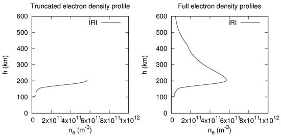
Figure 1.
Comparison between a representative ionosonde density profile (left), and a full density profile (right).
2.1. Nearest Neighbour
The nearest neighbour method is used to perform regression or classification tasks [52,53]. In regression, the goal is to infer a value of a continuous variable, i.e., inferring electron profiles or electron temperatures without discontinuities. The distances between different electron density 200-tuple profiles are estimated using Equation (1) and then used in order to determine the nearest neighbour. In 2022, Monte-Moreno et al. [54] proposed a global TEC forecast using the nearest neighbour method. In this study, a large number of 200-tuple inputs of electron density profiles and electron temperatures were used to construct the electron density and electron temperature inference models. In machine learning, the Manhattan or L1 distance used here is usually preferred over the Euclidean or L2 distance to avoid the curse of dimensionality in high-dimensional space, where traditional indexing and algorithmic techniques fail from an efficiency and/or effectiveness perspective [55,56]. The distance between two respective electron density profiles or electron temperature profiles A and B is determined using the following equation:
where (total number of entries in the training and validation sets), and and are the components of A and B tuples, respectively. The denominator in Equation (1) is introduced to prevent large overestimations in the inferences [57].
2.2. Radial Basis Function
The Radial Basis Function method is a regression method that performs interpolations of dependent variables at locations in a multi-dimensional space from selected reference points, also known as centres [57,58,59,60,61]. The RBF method generally does not require many centres to construct accurate models. Computer-based or synthetic-based inferences require a large number of data entries/nodes for the training and validation of the model. In this study, the number of centres varies between 8 and 12. As with the nearest neigbour approach, the independent input data set consists of X = () and the inferred dependent densities are in 200-tuple arrays Y calculated mathematically using the equation below:
where G is the interpolating function, are the interpolation coefficients determined from (2) by optimizing the selected loss function when the model is applied to the training and validation sets, X represents the independent input and represents the N centres. The interpolation coefficients are the solutions of the following system of linear equations:
As indicated by the argument of the function in Equations (2) and (3), RBFs depend on the distance (Euclidean in our study), which is denoted as . This distance dependence is the reason why those functions are called Radial Basis Functions. The interpolating function G can either be local or global and have different types as given below,
where and c are adjustable parameters for accuracy maximization by minimizing the loss function on the training and validation sets.
Among the above equations, Equations (6) and (7), known as polyharmonic spline functions, are examples of global functions whereas Equations (4) (Gaussian function) and (5) (inverse quadric funtion) are examples of local functions. In this study, the local equation given by (4) was used to construct the RBF model. Global functions vanish at the centre but are finite elsewhere, whereas local functions are non-zero at the centre where they are defined but tend to zero far from their centres. Using global functions, the regression of the dependent variable Y will be calculated by combining all the centres. However, with local functions , the determination of the dependent variable Y at a given n-tuple X is evaluated mostly from nearest neighbours in the set of all the centres. The choice of local or global functions in regression depends on the specifics of the problem, the number of centres, and the accuracy required. With a few centres, global functions are preferred to local ones, whereas local functions are preferred when there are many centres. Another consideration is the distribution of centres in the multivariate space, in order to optimise inference accuracy [62].
2.3. Loss Function
Finally, a key component of these regression techniques is the loss, or cost function. This is the function that quantifies the discrepancy between an inference and the known data from the training set. Training an inference model consists of minimising the loss function of a given data set. The loss function must generally have the following properties:
- 1.
- it must be nonnegative;
- 2.
- if the inferred data match the modelled ones, the loss function vanishes;
- 3.
- the loss function increases as the discrepancy between inferred and known training data increases.
Various mathematical expressions can be used to evaluate the loss function, for instance:
- (1)
- the Maximum Absolute Error (MAE)
- (2)
- the maximum absolute relative error (MARE)
- (3)
- the Root Mean Square Error (RMSE)
- (4)
- the Root Mean Square Relative Error (RMSRE)where N is the number of entries in the training and validation sets, and refer to the input profile and inferred profile, respectively. In this work, 200-tuple profiles from the IRI-2020 model or the ISR observations are used for training and testing the NNB and RBF models. The type of loss function used with the nearest neighbour model is the maximum relative absolute error in Equation (9), whereas the RBF model estimates the accuracy with the Root Mean Square Relative Error given by Equation (11). Maximum relative absolute error is better for Laplacian errors (larger errors) and more sensitive to outliers, while is better for normal or Gaussian errors (small errors) and less sensitive to outliers [63].
3. Results
As mentioned in previous sections, the results were obtained using ionosonde-like profiles truncated from IRI-2020 and two multivariate regression models (NNB and RBF). The inference results are discussed in two groups: the first results are for electron density inferences, and the second results are for the electron temperature profiles. The two regression models were assessed by applying them to 10 randomly selected cases. The best inferences among these 10, referred to as the “best inferences”, correspond to the cases for which the loss functions are the smallest. Conversely, the cases for which the loss functions are the largest are referred to as the “worst inferences”. The comparisons between these inferences and their known profiles are presented as a visual cue to assess the accuracy of the inference methods considered, as well as in the form of tables showing maximum absolute relative errors for both NNB and RBF models.
3.1. Inference of Electron Density Profiles with NNB and RBF Models
In order to illustrate the accuracy of both the NNB and RBF models, the best and worst inferences for each model are considered and compared for discussion. Figure 2 represents the best inference for the NNB model, while Figure 3 also shows the worst inference for the NNB model. Similarly, Figure 4 represents the best inference for the RBF model, and Figure 5 shows the worst inference for the same model.
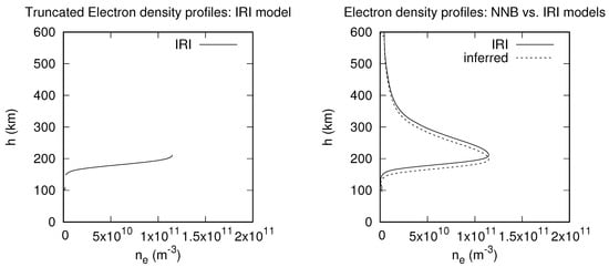
Figure 2.
Truncated (left) and best-inference (right) profiles inferred with NNB model compared with the corresponding IRI density profile.
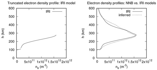
Figure 3.
Truncated (left) and worst-inference (right) profiles inferred with NNB model.
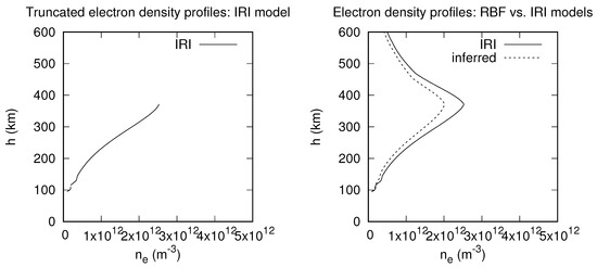
Figure 4.
Truncated (left) and best-inference (right) profiles inferred with RBF model.
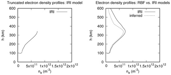
Figure 5.
Truncated (left) and worst-inference (right) profiles inferred with RBF model.
It can be seen in Figure 2 above that the NNB model’s inference almost matches the IRI electron profile values at higher altitudes from 400 km and above. However, the NNB model could not infer well the peak electron number densities of E-layer (NmE ). The deviations become larger in the E and F regions from around 95 km to 400 km. This good inference above the hmF2 region may suggest that NNB would be a good candidate to infer plasmaspheric electron densities, which would be compared with satellite (GPS) data. One can notice a slight translation of the IRI electron density against the inferred electron density from around 150 km to 300 km, which shifts the hmF2 from 180 km to 220 km at NmF2 . Another observation is that in the best inference, NNB only overestimates the electron density values below the peak values in the F region from 95 km to around 200 km and then changes the trend to underestimate them above it from 200 km to 400 km.
On the other hand, for the worst inference with the NNB model, the electron densities are largely overestimated below the F region peak ( ) from around 115 km to 260 km. Above the F region, the electron densities are underestimated from about 260 km to 340 km and again from 470 km to 600 km, whereas another overestimation is observed from 340 km to 470 km. It is worth mentioning that NNB models mostly follow the usual trend of electron density profiles for both the best and worst inferences.
Figure 4 shows the best inference from the RBF model. This model underestimates the electron densities at altitudes from around 135 km to 600 km. However, the RBF’s best inference is better able to reconstruct the density peak in the E region than the NNB model. On the other hand, the RBF’s best inference largely underestimates the electron densities around the F-region peak (NmF2 ), while the NNB model does not. This observation suggests that inferences can potentially be improved by combining both NNB and RBF models.
Figure 5 above suggests again that the RBF model yields good inferences of electron densities at lower altitudes, even in the E region layer. Given that the E region normally displays a single peak (hmE), it would be interesting to train and validate the RBF model with data on days with pronounced E sporadic to ascertain its accuracy in the E region. Yu et al. [64] have recently developed a deep learning model for E sporadic that achieves a significantly better performance with a correlation coefficient of r = 0.87 between RO observations and predictions.
Table 1 shows the values of maximum absolute relative error and their corresponding altitudes at which they occur for both best and worst electron density profile inferences using NNB and RBF models.

Table 1.
Maximum absolute relative error and corresponding altitudes for electron density profile inferences with NNB and RBF models.
It is observed that the NNB model has smaller values than the RBF model for both best and worst inferences. The altitudes at which values are large are generally found above the hmF2, except for the best inference of electron density profiles at 145 km. For the best inference from the NNB model, the maximum is almost constant and smaller from hmE through hmF2 to around 300 km (seen in (Figure 2)). Table 1 also shows that the corresponding altitudes for electron density profiles are larger (415 km and 420 km) for worst inference cases and smaller (145 km and 360 km) for the best inferences for NNB and RBF, respectively.
3.2. Inference of Electron Temperature Profiles with NNB and RBF Models
It is found that both NNB and RBF models perform well at lower altitudes for both the best and worst inferences. Bilitza et al. [65] were among the first researchers to model the ionospheric temperature profiles with the IRI-79 model. They found that IRI electron temperatures were not well estimated between 300 and 600 km, which is the same range in which NNB and RBF models mostly underestimate or overestimate the inferred temperatures.
Figure 6 shows the best inference of electron temperature profiles with the NNB model. It is observed that the NNB model reconstructed the electron temperature values from 95 km to 150 km well, with a steadily increasing underestimation at higher altitudes. From 260 km to 600 km, the slope or shift of the IRI against the inferred electron profiles is almost uniform, and this feature has also been observed in the inference of electron density profiles with the NNB model as seen in Figure 2.
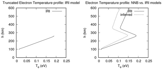
Figure 6.
Best inference of the electron temperature with NNB model.
Figure 7 shows a worst inference for the NNB model and shows again that temperature inferences made with NNB are only reliable at lower altitudes up to around 200 km, as for the best inference. From around 300 km to 600 km, the NNB model largely overestimates the inferred electron temperature values. In this case, even the altitude at which the electron temperature is maximum (0.2 eV) is shifted down from 260 km (IRI) to just 220 km (inferred) compared to the best inference, where this altitude is almost the same (250 km) for both IRI and inferred temperature profiles.
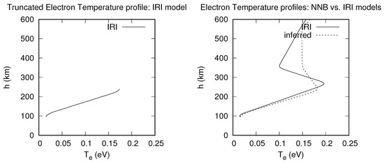
Figure 7.
Worst inference of electron temperature profiles inferred with the NNB model.
Figure 8 illustrates the best inference for the RBF model. The RBF model shows a near-perfect match at all altitudes from 95 km to 600 km. The deviation between IRI and inferred values is also small. A slight underestimation and overestimation are only noticeable from 350 km to 600 km.
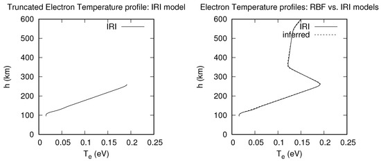
Figure 8.
Plot of best temperature inference inferred with the RBF model.
However, a significant deviation is observed at altitudes above 400 km for the worst inference in Figure 9. RBF slightly overestimates the hmF peak (265 km) with a deviation of almost 0.01 eV. The underestimation becomes large from the second peak (0.12 eV), but the model inferred well the electron temperature at the second peak altitude (h ∼ 350 km), with a deviation of about 0.02 eV.

Figure 9.
Plot of worst temperature inference with RBF model.
The values of maximum absolute relative error and their corresponding altitudes for the electron temperature profile inferences are given in Table 2 for the NNB and RBF inferences. Considering the best cases for both models, it can be seen that the RBF model ( = 0.01) infers the electron temperature profiles better than the NNB model ( = 0.27). Again, it is noticed that the corresponding altitudes are at or above hmF2 as seen in Table 2. As for the electron density profiles, Table 2 shows that the corresponding altitudes for the electron temperature profiles for the worst inference cases (350 km for NNB and 420 km for RBF) are higher than for the best inference cases (255 km for NNB and 360 km for RBF).
Table 2.
Maximum absolute relative error and corresponding altitudes for electron temperature profile inferences with the NNB and RBF models.
4. Conclusions
In conclusion, both NNB and RBF models are able to reproduce the trend of the ionospheric electron density profiles well, except at peak densities of the E and F regions, where there is usually either a larger underestimation or overestimation of the inferred profiles. NNB and RBF models generally infer the electron density profiles and electron temperature profiles with a larger from hmF2 to 600 km, except for the best inferences. Corresponding altitudes for both electron density and temperature profiles for the worst inference profiles are higher than for the best inference profiles. The two models can be used to infer the electron density and temperature profiles below the maximum densities and peak temperatures. Electron density profiles are observed to be well inferred with the NNB model for the best and worst inferences than with the RBF model. On the other hand, RBF infers the electron temperature profiles better than the NNB model. An important finding of this study is that standard machine learning regression techniques, optimised to extend electron density profiles beyond altitudes accessible to ionosonde measurements, can also be used to infer electron temperature profiles using the same electron density profiles. The two models considered here have been trained and validated with synthetic data constructed using the IRI 2020 model. A question remains as to how well these model inferences will compare with actual measurements made in situ with satellites, or remotely with arrays of GPS signals or incoherent scatter radars; these considerations will be addressed in future studies.
Author Contributions
Conceptualization, R.M.; Methodology, J.d.D.N.; Software, R.M.; Validation, J.d.D.N.; Data curation, J.d.D.N.; Writing—original draft, J.d.D.N.; Writing—review & editing, R.M.; Supervision, R.M.; Funding acquisition, R.M. All authors have read and agreed to the published version of the manuscript.
Funding
This research was funded by the Natural Sciences and Engineering Research Council of Canada.
Institutional Review Board Statement
Not applicable.
Informed Consent Statement
Not applicable.
Data Availability Statement
IRI 2020 data are available at https://ccmc.gsfc.nasa.gov/models/IRI~2020/, accessed on 2 September 2024.
Acknowledgments
The authors of this article thank the Natural Sciences and Engineering Research Council of Canada and the University of Alberta for their financial support.
Conflicts of Interest
The authors declare no conflicts of interest.
Abbreviations
The following abbreviations are used in this manuscript:
| NNB | Nearest Neighbour |
| RBF | Radial Basis Function |
| IRI | International Reference Ionosphere |
| E-CHAIM | Empirical Canadian High Arctic Ionospheric Model |
| GPS | Global Positioning System |
| AfriTEC | Africa Total Electron Content |
| ISR | Incoherent Scattering Radars |
| OSSEs | Observation System Simulation Experiments |
| TEC | Total Electron Content |
| COSMIC | Constellation Observing System for Meteorology, Ionosphere and Climate |
| RIOMETER | Relative Ionospheric Opacity Meter for Extra-Terrestrial Emissions of Radio noise |
| RO | Radio Occultation |
| hmE | Height at Maximum E layer |
| hmF2 | Height at Maximum F2 layer |
| NmE | Maximum electron density in E layer |
| NmF2 | Maximum electron density in F2 layer |
| GOES | Geostationary Operational Environmental Satellites |
References
- Appleton, E.V. Geophysical influences on the transmission of wireless waves. Proc. Phys. Soc. Lond. 1924, 37, 16D–22D. [Google Scholar] [CrossRef]
- Marconi, G. Radio telegraphy. J. Am. Inst. Electr. Eng. 1922, 41, 561–570. [Google Scholar] [CrossRef]
- Breit, G.; Tuve, M.A. A test of the existence of the conducting layer. Phys. Rev. 1926, 28, 554–575. [Google Scholar] [CrossRef]
- Yao, M.; Chen, G.; Zhao, Z.; Wang, Y.; Bai, B. A novel low-power multifunctional ionospheric sounding system. IEEE Trans. Instrum. Meas. 2011, 61, 1252–12591. [Google Scholar] [CrossRef]
- Lei, J.; Liu, L.; Wan, W.; Zhang, S. Variations of electron density based on long-term incoherent scatter radar and ionosonde measurements over millstone hill. Radio Sci. 2015, 40, RS2008. [Google Scholar] [CrossRef]
- Olsen, N.; Friis-Christensen, E.; Floberghagen, R.; Alken, P.; Beggan, C.D.; Chulliat, A.; Doornbos, E.; Da Encarnação, J.T.; Hamilton, B.; Hulot, G.; et al. The Swarm Satellite Constellation Application and Research Facility (SCARF) and Swarm data products. Earth Planets Space 2013, 65, 1189–1200. [Google Scholar] [CrossRef]
- Ware, R.; Exner, M.; Feng, D.; Gorbunov, M.; Hardy, K.; Herman, B.; Kuo, Y.; Meehan, T.; Melbourne, W.; Rocken, C.; et al. Gps sounding of the atmosphere from low earth orbit: Preliminary results. Bull. Am. Meteorol. Soc. 1996, 77, 19–40. [Google Scholar] [CrossRef]
- Anthes, R.A. Exploring earth’s atmosphere with radio occultation: Contributions to weather, climate and space weather. Atmos. Meas. Tech. 2011, 4, 1077–1103. [Google Scholar] [CrossRef]
- De Dieu Nibigira, J.; Venkat, D.R.; Prasad, G. Analysis of ionospheric GPS-TEC variability over Uganda IGS station during descending phase of 24th solar cycle, 2018 year. Int. J. Sci. Technol. Res. 2019, 8, 3947–3950. [Google Scholar]
- Cheng, P.H.; Morton, Y.J. Observation of large-scale traveling ionospheric disturbances in the topside ionosphere using POD TEC from multiple LEO satellites constellations. J. Geophys. Res. Space Phys. 2025, 130, e2024JA033293. [Google Scholar] [CrossRef]
- Siskind, D.E.; Jones, M., Jr.; Reep, J.W.; Drob, D.P.; Samaddar, S.; Bailey, S.M.; Zhang, S.R. Tests of a new solar flare model against D and E region ionosphere data. Space Weather 2022, 20, e2021SW003012. [Google Scholar] [CrossRef]
- Anderson, D.N.; Kintner, P.M.; Kelley, M.C. Inference of equatorial field-line-integrated electron density values using whistlers. J. Atmos. Terr. Phys. 1985, 47, 989–997. [Google Scholar] [CrossRef]
- Hughes, J.; Forsythe, V.; Blay, R.; Azeem, I.; Crowley, G.; Wilson, W.J.; Dao, E.; Colman, J.; Parris, R. On constructing a realistic truth model using ionosonde data for observation system simulation experiments. Radio Sci. 2022, 57, e2022RS007508. [Google Scholar] [CrossRef]
- He, J.; Yue, X.; Astafyeva, E.; Le, H.; Ren, Z.; Pedatella, N.M.; Ding, F.; Wei, Y. Global gridded ionospheric electron density derivation during 2006–2016 by assimilating COSMIC TEC and its validation. J. Geophys. Res. Space Phys. 2022, 127, e2022JA030955. [Google Scholar] [CrossRef]
- Giovanni, G.D.; Radicella, S.M. An analytical model of the electron density profile in the ionosphere. Adv. Space Res. 1990, 10, 27–30. [Google Scholar] [CrossRef]
- McKay, D.; Vierinen, J.; Kero, A.; Partamies, N. On the determination of ionospheric electron density profiles using multi-frequency riometry. Geosci. Instrum. Method. Data Syst. 2022, 11, 25–35. [Google Scholar] [CrossRef]
- Sibanda, P.; McKinnell, L. Topside ionospheric vertical electron density profile reconstruction using GPS and ionosonde data: Possibilities for south africa. Ann. Geophys. 2011, 9, 229–236. [Google Scholar] [CrossRef][Green Version]
- Alzubaidi, L.; Bai, J.; Al-Sabaawi, A.; Santamaría, J.; Albahri, A.S.; Al-Dabbagh, B.S.N.; Fadhel, M.A.; Manoufali, M.; Zhang, J.; Al-Timemy, A.H.; et al. A survey on deep learning tools dealing with data scarcity: Definitions, challenges, solutions, tips, and applications. J. Big Data 2023, 10, 46. [Google Scholar] [CrossRef]
- Lin, Y.; Fang, H.; Duan, D.; Huang, H.; Xiao, C.; Ren, G.; Li, C.; Zhou, C. Enhancing deep learning ionospheric modeling with solar radiation and flare classes. J. Geophys. Res. Space Phys. 2025, 130, e2024JA033319. [Google Scholar] [CrossRef]
- Weng, J.; Liu, Y.; Wang, J.A. Model-Assisted Combined Machine Learning Method for Ionospheric TEC Prediction. Remote Sens. 2023, 15, 2953. [Google Scholar] [CrossRef]
- Zhang, R.; Li, H.; Shen, Y.; Yang, J.; Li, W.; Zhao, D.; Hu, A. Deep Learning Applications in Ionospheric Modeling: Progress, Challenges, and Opportunities. Remote Sens. 2025, 17, 124. [Google Scholar] [CrossRef]
- Kates-Harbeck, J.; Svyatkovskiy, A.; Tang, W. Predicting disruptive instabilities in controlled fusion plasmas through deep learning. Nature 2019, 568, 526–531. [Google Scholar] [CrossRef] [PubMed]
- Kim, S.; Shousha, R.; Yang, S.; Hu, Q.; Hahn, S.; Jalalvand, A.; Park, J.K.; Logan, N.C.; Nelson, A.O.; Na, Y.S.; et al. Highest fusion performance without harmful edge energy bursts in tokamak. Nat. Commun. 2024, 15, 3990. [Google Scholar] [CrossRef]
- Döpp, A.; Eberle, C.; Howard, S.; Irshad, F.; Lin, J.; Streeter, M. Data-driven science and machine learning methods in laser–plasma physics. High Power Laser Sci. Eng. 2025, 11, e55. [Google Scholar] [CrossRef]
- Faraji, F.; Reza, M. Machine learning applications to computational plasma physics and reduced-order plasma modeling: A perspective. J. Phys. D Appl. Phys. 2025, 58, 102002. [Google Scholar] [CrossRef]
- Salimov, B.G.; Yasyukevich, Y.V.; Vesnin, A.M.; Bykov, A.E.; Zhang, B.; Ratnam, D.V. Machine learning total electron content models based on F10.7. Adv. Space Res. 2025, 76, 317–330. [Google Scholar] [CrossRef]
- Habarulema, J.B.; Okoh, D.; Burešová, D.; Rabiu, B.; Tshisaphungo, M.; Kosch, M.; Häggström, I.; Erickson, P.J.; Milla, M.A. A global 3-D electron density reconstruction model based on radio occultation data and neural networks. J. Atmos. Sol.-Terr. Phys. 2022, 221, 105702. [Google Scholar] [CrossRef]
- Habarulema, J.B.; Okoh, D.; Burešová, D.; Rabiu, B.; Scipión, D.; Häggström, I.; Erickson, P.J.; Milla, M.A. A storm-time global electron density reconstruction model in three-dimensions based on artificial neural networks. Adv. Space Res. 2019, 124, 4639–4657. [Google Scholar] [CrossRef]
- Hu, A.; Carter, B.; Currie, J.; Norman, R.; Wu, S.; Zhang, K. A Deep Neural Network Model of Global Topside Electron Temperature Using Incoherent Scatter Radars and Its Application to GNSS Radio Occultation. J. Geophys. Res. Space Phys. 2020, 125, e2019JA027263. [Google Scholar] [CrossRef]
- Bilitza, D.; Truhlik, V.; Yoshihara, O.; Moldwin, M.B. Development and Improvement of the International Reference Ionosphere with special emphasis on the topside and extension to the plasmasphere. Ann. Geophys. 2024, 67, SA443. [Google Scholar] [CrossRef]
- Nibigira, J.D.D.; Ratnam, D.V.; Sivavaraprasad, G. Performance analysis of IRI-2016 model TEC predictions over Northern and Southern Hemispheric IGS stations during descending phase of solar cycle 24. Acta Geophys. 2021, 69, 1509–1527. [Google Scholar] [CrossRef]
- Endeshaw, L. Comparison of NeQuick and IRI Models with Ionosonde Data for Ionospheric Electron Density Measurements. Geomagn. Aeron. 2025, 1–15. [Google Scholar] [CrossRef]
- Jayachandran, P.T.; Langley, R.B.; MacDougall, J.W.; Mushini, S.C.; Pokhotelov, D.; Hamza, A.M. Canadian high arctic ionospheric network (chain). Radio Sci. 2009, 44, 342–351. [Google Scholar] [CrossRef]
- Nibigira, J.D.D.; Ratnam, D.; Sivakrishna, K. Performance analysis of Nequick-G, IRI-2016, IRI-Plas 2017 and AfriTEC models over the African region during the geomagnetic storm of March 2015. Geomagn. Aeron. 2023, 63, S83–S98. [Google Scholar] [CrossRef]
- Larson, B.; Koustov, A.V.; Themens, D.R.; Gillies, R.G. Ionospheric electron density over Resolute Bay according to E-CHAIM model and RISR radar measurements. Adv. Space Res. 2023, 71, 2759–2769. [Google Scholar] [CrossRef]
- Chen, Z.; An, B.; Liao, W.; Wang, Y.; Tang, R.; Wang, J.; Deng, X. Ionospheric Electron Density Model by Electron Density Grid Deep Neural Network (EDG-DNN). Atmosphere 2023, 14, 810. [Google Scholar] [CrossRef]
- Zakharenkova, I.; Cherniak, I.; Gleason, S.; Hunt, D.; Freesland, D.; Krimchansky, A.; McCorkel, J.; Ramsey, G.; Chapel, J. Statistical validation of ionospheric electron density profiles retrievals from GOES geosynchronous satellites. J. Space Weather Space Clim. 2023, 13, 23. [Google Scholar] [CrossRef]
- Köhnlein, W. A model of the electron and ion temperatures in the ionosphere. Planet. Space Sci. 1986, 34, 609–630. [Google Scholar] [CrossRef]
- Matta, M.; Galand, M.; Moore, L.; Mendillo, M.; Withers, P. Numerical simulations of ion and electron temperatures in the ionosphere of Mars: Multiple ions and diurnal variations. Icarus 2014, 227, 78–88. [Google Scholar] [CrossRef]
- Pignalberi, A.; Giannattasio, F.; Truhlik, V.; Coco, I.; Pezzopane, M.; Alberti, T. Investigating the main features of the correlation between electron density and temperature in the topside ionosphere through swarm satellites data. J. Geophys. Res. Space Phys. 2024, 129, e2023JA032201. [Google Scholar] [CrossRef]
- Su, F.; Wang, W.; Burns, A.G.; Yue, X.; Zhu, F. The correlation between electron temperature and density in the topside ionosphere during 2006–2009. J. Geophys. Res. Space Phys. 2015, 120, 10724–10739. [Google Scholar] [CrossRef]
- Grant, S.W.; Hickey, G.L.; Head, S.J. Statistical primer: Multivariable regression considerations and pitfalls. Eur. J. Cardio-Thorac. Surg. 2019, 55, 179–185. [Google Scholar] [CrossRef] [PubMed]
- Samuel, A.L. Some studies in machine learning using the game of checkers. IBM J. Res. Dev. 1959, 3, 210–229. [Google Scholar] [CrossRef]
- Aggarwal, C. Neural Networks and Deep Learning; Springer: Cham, Switzerland, 2018; Volume 978, p. 3. [Google Scholar] [CrossRef]
- Mallika, I.L.; Ratnam, D.V.; Ostuka, Y.; Sivavaraprasad, G.; Raman, S. Implementation of hybrid ionospheric TEC forecasting algorithm using PCA-NN method. IEEE J. Sel. Top. Appl. Earth Obs. Remote Sens. 2018, 12, 371–381. [Google Scholar] [CrossRef]
- Azari, A.; Biersteker, J.B.; Dewey, R.M.; Doran, G.; Forsberg, E.J.; Harris, C.D.K.; Kerner, H.R.; Skinner, K.A.; Smith, A.W.; Amini, R.; et al. Integrating Machine Learning for Planetary Science: Perspectives for the Next Decade. Bull. AAS 2021, 53, 2023–2032. [Google Scholar] [CrossRef]
- Han, Y.; Wang, L.; Fu, W.; Zhou, H.; Li, T.; Chen, R. Machine learning-based short-term GPS TEC forecasting during high solar activity and magnetic storm periods. IEEE J. Sel. Top. Appl. Earth Obs. Remote Sens. 2022, 15, 115–126. [Google Scholar] [CrossRef]
- Abolfathi, M.; Inturi, S.; Banaei-Kashani, F.; Jafarian, J.H. Toward enhancing web privacy on HTTPS traffic: A novel SuperLearner attack model and an efficient defense approach with adversarial examples. Comput. Secur. 2024, 139, 103673. [Google Scholar] [CrossRef]
- Dittmann, T.T.; Chang, H.; Morton, Y. Multiclass Machine Learning in Low Cost CubeSat GNSS Radio Occultation Profiles. Presented at the AGU Fall Meeting 2024, Washington, DC, USA, 9–13 December 2024. [Google Scholar]
- Azari, A.R.; Lockhart, J.W.; Liemohn, M.W.; Jia, X. Incorporating physical knowledge into machine learning for planetary space physics. Front. Astron. Space Sci. 2020, 7, 36. [Google Scholar] [CrossRef] [PubMed]
- Sarker, I. Machine learning: Algorithms, real-world applications and research directions. SN Comput. Sci. 2021, 2, 160. [Google Scholar] [CrossRef]
- Wang, J.; Neskovic, P.; Cooper, L.N. An adaptive nearest neighbor algorithm for classification. In Proceedings of the 2005 International Conference on Machine Learning and Cybernetics, Guangzhou, China, 18–21 August 2005; Volume 5, pp. 3069–3074. [Google Scholar] [CrossRef]
- Gu, X.; Akoglu, L.; Rinaldo, A. Statistical analysis of nearest neighbor methods for anomaly detection. In Proceedings of the Advances in Neural Information Processing Systems 32 (NeurIPS 2019), Vancouver, BC, Canada, 8–14 December 2019. [Google Scholar]
- Monte-Moreno, E.; Yang, H.; Hernández-Pajares, M. Forecast of the global TEC by nearest neighbour technique. Remote Sens. 2022, 14, 1361. [Google Scholar] [CrossRef]
- Aggarwal, C.; Hinneburg, A.; Keim, D. On the surprising behavior of distance metrics in high dimensional space. In Database Theory—ICDT 2001, Proceedings of the 8th International Conference on Database Theory, London, UK, 4–6 January 2001; Van den Bussche, J., Vianu, V., Eds.; Lecture Notes in Computer Science; Springer: Berlin/Heidelberg, Germany, 2001; Volume 1973. [Google Scholar] [CrossRef]
- Bellman, R. Dynamic programming. Science 2019, 153, 34–37. [Google Scholar] [CrossRef] [PubMed]
- Marchand, R.; Shahsavani, S.; Sanchez-Arriaga, G. Beyond analytic approximations with machine learning inference of plasma parameters and confidence intervals. J. Plasma Phys. 2023, 89, 905890111. [Google Scholar] [CrossRef]
- Huang, Z.; Yuan, H. Ionospheric single-station TEC short-term forecast using RBF neural network. Radio Sci. 2014, 49, 283–292. [Google Scholar] [CrossRef]
- Olowookere, A.; Marchand, R. A new technique to infer plasma density, flow velocity, and satellite potential from ion currents collected by a segmented langmuir probe. IEEE Trans. Plasma Sci. 2022, 50, 3774–3786. [Google Scholar] [CrossRef]
- Liu, G.; Marholm, S.; Eklund, A.; Clausen, L.; Marchand, R. m-NLP inference models using simulation and regression techniques. J. Geophys. Res. Space Phys. 2023, 128, e2022JA030835. [Google Scholar] [CrossRef]
- Tang, S.; Huang, Z.; Yuan, H. Improving regional ionospheric TEC mapping based on RBF interpolation. Adv. Space Res. 2021, 7, 722–730. [Google Scholar] [CrossRef]
- Liu, G.; Marchand, R. Inference of m-NLP data using radial basis function regression with center-evolving algorithm. Comput. Phys. Commun. 2022, 280, 108497. [Google Scholar] [CrossRef]
- Hodson, T.O. Root mean square error (RMSE) or mean absolute error (MAE): When to use them or not. Geosci. Model Dev. 2022, 15, 5481–5487. [Google Scholar] [CrossRef]
- Yu, B.; Tian, P.; Xue, X.; Scott, C.J.; Ye, H.; Wu, J.; Yi, W.; Chen, T.; Dou, X. Modelling of ionospheric temperature profiles. Adv. Space Res. 2024, 9, 10–19. [Google Scholar] [CrossRef]
- Bilitza, D.; Brace, L.H.; Theis, R.F. Modelling of ionospheric temperature profiles. Adv. Space Res. 2019, 5, 53–58. [Google Scholar] [CrossRef]


Disclaimer/Publisher’s Note: The statements, opinions and data contained in all publications are solely those of the individual author(s) and contributor(s) and not of MDPI and/or the editor(s). MDPI and/or the editor(s) disclaim responsibility for any injury to people or property resulting from any ideas, methods, instructions or products referred to in the content. |
© 2025 by the authors. Licensee MDPI, Basel, Switzerland. This article is an open access article distributed under the terms and conditions of the Creative Commons Attribution (CC BY) license (https://creativecommons.org/licenses/by/4.0/).