An Algorithm for Structural Optimization of Intelligent Radio Communication System

Abstract

This article develops a structural optimization algorithm for designing intelligent and adaptive radio communication systems. In modern tactical crisis operations characterized by high environmental dynamics and intense electromagnetic countermeasures, as well as in emergency response networks, static communication planning approaches prove increasingly ineffective. The paper introduces a stable normalization method for performance estimates and a mechanism for rapid algorithmic adaptation to shifting operational priorities. A key feature of the proposed approach is an adaptive objective function based on the weighted sum of normalized criteria for survivability, noise immunity, and reliability. The use of weighting coefficients enables rapid adjustment of optimization priorities in response to extreme conditions, whilst the application of a normalization method based on threshold values ensures the stability and comparability of evaluations. It is practical that the proposed algorithm will enable the synthesis of functionally stable and robust structures, thereby enhancing the reliability of command and control of forces and assets in both mission-critical operations and civil crisis situations.

1. Introduction

In modern crisis situations, achieving objectives is inextricably linked to gaining an information advantage. The physical foundation of command and control that enables this advantage to be realized is the communications system. The success of any operation depends directly on its technological level, quality, and operational effectiveness [1,2,3]. The operation of modern intelligent and adaptive radio communication systems takes place in conditions of crisis situations, the main features of which are the highly dynamic nature of the changing situation, as well as the unpredictable disruption of control system elements. The opposing sides actively employ intense electromagnetic interference (EMI) means with the aim of disrupting or completely disorganising command and control.

Scientific publications indicate the active use of adaptive network solutions, in particular Mobile Ad-hoc Networks (MANET) and mesh structures. In these architectures, network nodes can autonomously change their topology, which is critically important in crisis conditions characterized by rapid, unpredictable changes and threats. Research [4,5] demonstrates the potential for applying artificial intelligence algorithms, in particular, genetic algorithms (GA), neural network models, and swarm intelligence algorithms for dynamic route management, adaptation to environmental changes, and minimisation of delays.

Recent studies published in leading international scientific journals demonstrate significant interest in optimizing communication networks under conditions of intense electromagnetic interference. A significant number of recent works [6,7] focus on the application of meta-heuristic methods to solve problems of multi-constraint routing and topology control. Thus, a number of foreign studies [8,9] propose approaches to restoring network connectivity based on intelligent modifications of routing protocols. Another area of research [10,11] focuses on ensuring the stability of communication channels by estimating the signal-to-interference ratio (SINR) in dynamic scenarios involving unmanned platforms.

Particular attention is drawn to the experience of building self-configuring networks using frequency hopping spread spectrum (FHSS), which provides enhanced resistance to jamming and interception. In such systems, radio channels change according to a pseudo-random principle, and frequency sequence encryption is used, which significantly complicates the work of the enemy’s intense electromagnetic interference (EMI). However, the practical implementation of FHSS requires high synchronization between nodes, resulting in a trade-off between quality of service (QoS) and energy consumption and throughput. The issue of constructing communication systems has been addressed in numerous works [1,2,12,13,14], where it is proposed to represent their structure as a set of interconnected functional subsystems, formalized using mathematical tools [15].

Nevertheless, a detailed analysis shows that existing solutions only partially address optimization problems or are tailored to specific conditions. Most of them remain tied to static planning, focusing exclusively on the protocol level or on static impact models, whilst ignoring the complex effects of physical disruption or hardware degradation on nodes. Furthermore, when using multi-criteria optimization in modern research, linear normalization relative to the sample’s minimum and maximum values is often applied, making it impossible to objectively compare results over time. Under such conditions, traditional methods for designing communication system architecture become ineffective, as they cannot respond flexibly to changes in threats and operational tasks.

This raises the pressing scientific and applied challenge of developing a methodology and toolkit for the automated synthesis of a radio communication structure that is not merely functional, but optimal for the specific conditions and priorities of the mission. The scientific novelty lies in a comprehensive approach to threat mitigation through the simultaneous optimization of network survivability, noise immunity, and reliability using a seven-step procedural logic to evaluate the objective function and dynamically prune vulnerabilities. Specifically, the simulation verification results demonstrate that the algorithm successfully isolates compromised clusters, enhancing overall network resilience by preventing cascading failures during targeted attacks.

This study aims to create a flexible tool for the automated identification of network topologies that best align with mission-specific priorities, whether for emergency response or rescue operations. A genetic algorithm is proposed to address this problem. The scientific novelty lies in a comprehensive approach to threat mitigation through the simultaneous optimization of network survivability, noise immunity, and reliability.

The main scientific contribution of this research lie in the following:

-

Comprehensive consideration of heterogeneous threats: Unlike most existing approaches that consider the impact of electromagnetic interference or physical degradation in isolation, the proposed algorithm optimizes the topology at the macro level simultaneously according to three criteria: survivability, noise immunity, and reliability [8,9,10,11]. This allows us to synthesize comprehensively protected structures.

-

Approach to normalization of the objective function: Instead of the classical linear minimax normalization, which is used in similar studies and is sensitive to new extrema, a normalization method based on expertly specified threshold and boundary values was applied. This ensures the stability of the function and allows us to objectively compare network configurations in dynamics without recalculating the entire sample.

-

Adaptability of evolutionary search: A mechanism for operational reconfiguration of the genetic algorithm by changing the weight coefficients of the objective function is proposed. This allows the system to not simply search for a mathematical optimum, but to generate robust (quasi-optimal) topologies that meet the priorities of a specific mission phase.

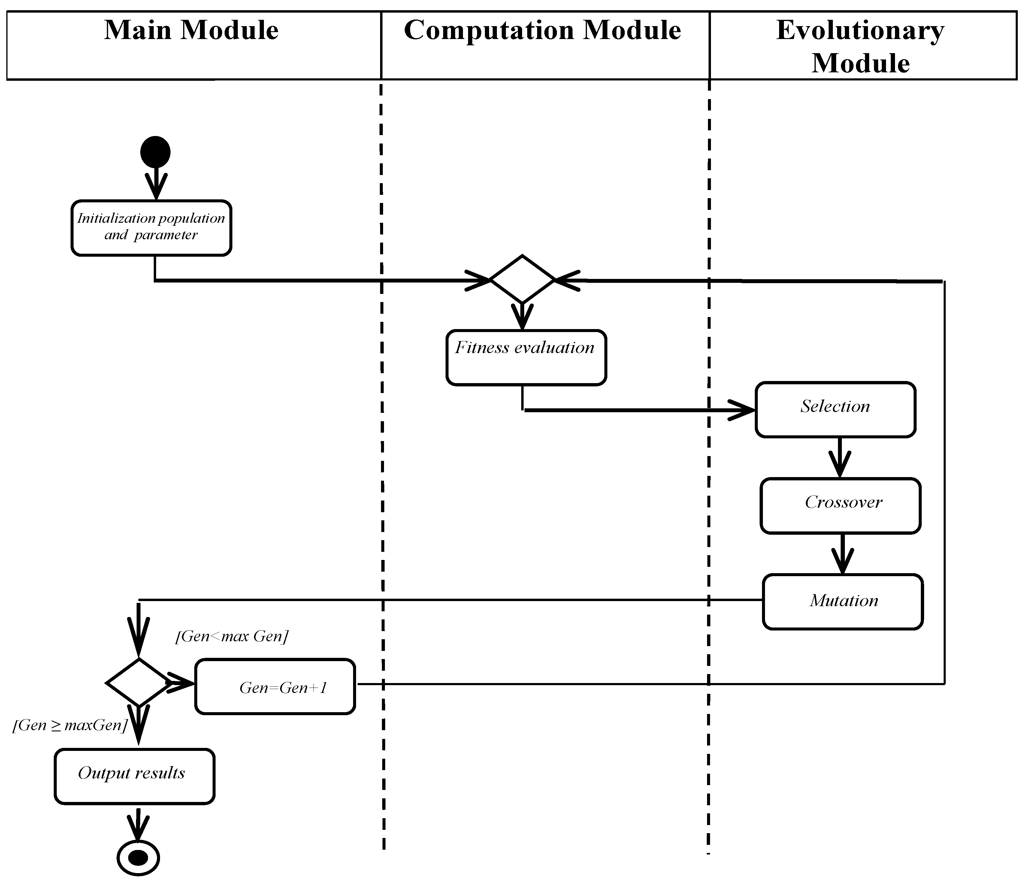
2. System Model

2.1. Graph Modeling and Constraints

The structure of a radio communication system can be represented mathematically as a graph $\mathrm{G}=\left\{V,E\right\}$.

$$\mathrm{G}=\left\{V,E\right\}.$$

(1)

where

G is the mathematical structure modeling the network.

V is the set of all organizational and technical units requiring communication.

E is the set of all theoretically possible connections, including both active and potential links.

The vertices (or nodes) of graph $\mathrm{V}$ represent the physical elements of the radio communication system. These include: radio communication nodes (centers), control points, individual mobile groups, or elements forming part of the radio communication system.

The edges of graph $\mathrm{E}$ represent the set of all possible communication channels between the nodes of the radio communication system. These may include radio networks and radio links, as well as connection lines to the backbone network.

Thus, the problem can be formulated as follows: for a given set of nodes V and a set of potentially possible communication channels between them $\mathrm{E}$, it is necessary to find a subgraph ${\mathrm{G}}^{\prime }=\left\{\mathrm{V},{\mathrm{E}}^{\prime }\right\}$, where ${\mathrm{E}}^{\prime }\in \mathrm{E}$, which maximizes the comprehensive performance metric, taking into account the priorities of the current mission. This subgraph ${\mathrm{G}}^{\prime }$ is the optimal structure of the communication system. It includes only that set of active communication channels (${\mathrm{E}}^{\prime }$) which maximizes the comprehensive performance metric (objective function $\mathrm{F}\left(\mathrm{C}\right)$) for the priorities of the current mission. Each possible network configuration (i.e., each possible subgraph ${\mathrm{G}}^{\prime }$) can also be represented as a binary chromosome, where each bit indicates the presence or absence of a specific communication channel in the structure. ‘1’ means that the channel is active (the edge belongs to ${\mathrm{E}}^{\prime }$), and ‘0’ means that it is inactive (the edge does not belong to ${\mathrm{E}}^{\prime }$).

The formal representation of a radio communication system as a graph provides a powerful mathematical tool for describing its topological structure. However, this representation is static in itself. It merely defines the set of all possible configurations, each of which is a subgraph. In highly dynamic deployment conditions, characterized by high dynamics and active enemy countermeasures, the key scientific and applied task lies not simply in description, but in selecting a single, optimal structure from a vast space of possible variants.

Such a choice cannot be arbitrary, as it requires a formalized, quantitative assessment of the quality of each potential configuration. To determine which network structure is objectively superior to another in the context of a specific mission, a comprehensive system of optimization criteria is applied. These criteria serve as metrics that allow the functional suitability of any subgraph to be assessed in terms of the key requirements for any communication system. They translate the abstract topology of the graph into measurable performance indicators. It is precisely through the prism of these criteria—survivability, noise immunity, and reliability—that the effectiveness of each structure can be quantitatively determined and a targeted search conducted for the one that best meets the set objectives.

An important feature of the objective function [16] is the impossibility of achieving, within a single process and with the same set of control factors, the maximum (minimum) value of two or more indicators. When formulating the optimization indicator, one must identify and incorporate all necessary constraints to obtain a suitable objective function.

The network is modeled as a directed graph. For eight nodes, a fully connected undirected graph contains 28 edges, and a directed graph contains 56 directed links. However, to account for real-world deployment constraints (e.g., terrain obstructions or maximum transmission ranges), 14 links are considered physically impossible a priori. Thus, the operational topology is defined by exactly 42 viable directed links, which form the 42-bit chromosome for the optimization process. A comprehensive system scenario diagram illustrating the spatial distribution and interference zones has been formulated to map these links. The optimization only searches within this physically feasible space.

2.2. Objective Function Formulation

A key element of the proposed algorithm is the adaptive objective function (fitness function) $\mathrm{F}\left(\mathrm{C}\right)$, which reduces the multi-parameter evaluation problem to a scalar form [15,16]. It calculates the quality of each potential network configuration (chromosome C) by finding the additive convolution (weighted sum) of three normalized criteria. These criteria—survivability, noise immunity, and reliability—are based on the fundamental requirements for the organization of radio communications [1,2,3].

The model’s flexibility and adaptability to the dynamics of environmental changes are achieved through weighting coefficients (${\mathrm{w}}_1,{\mathrm{w}}_2,{\mathrm{w}}_3$), the sum of which equals 1. In practice, these coefficients are set by experts (for example, by officials of the communications management body at the planning stage or based on the current task the Analytic Hierarchy Process (AHP) to ensure consistency) immediately before the mission is carried out or when its phase changes [1,14]. To ensure consistency in defining these coefficients, Saaty’s Analytic Hierarchy Process (AHP) and its associated ranking scales were formally applied. This guarantees that expert inputs regarding mission priorities are mathematically sound and consistent prior to running the optimization.

A key element of the proposed algorithm is the adaptive objective function (fitness function) $\mathrm{F}\left(\mathrm{C}\right)$, which evaluates the quality of each network configuration (chromosome C). It represents the weighted sum of three main criteria corresponding to the key requirements for communication systems. Adaptability is achieved by weighting coefficients (${\mathrm{w}}_1,{\mathrm{w}}_2,{\mathrm{w}}_3$), whose sum equals 1. These coefficients are set by experts prior to the mission and reflect its priorities. For example, for a reconnaissance mission, ${\mathrm{w}}_2$ (noise immunity) will be given the highest weight, whilst for commanding troops during an offensive, ${\mathrm{w}}_1$ (survivability) will be given the highest weight:

$$\mathrm{F}\left(\mathrm{C}\right)={\mathrm{w}}_1\cdot \overline{{\mathrm{K}}_{\mathrm{s}\mathrm{u}\mathrm{r}}}+{\mathrm{w}}_2\cdot \overline{{\mathrm{K}}_{\mathrm{i}\mathrm{m}\mathrm{m}}}+{\mathrm{w}}_3\cdot \overline{{\mathrm{K}}_{\mathrm{r}\mathrm{e}\mathrm{l}}}\to \mathrm{m}\mathrm{a}\mathrm{x}$$

(2)

where

${\mathrm{w}}_1,{\mathrm{w}}_2,{\mathrm{w}}_3$ are weighting coefficients that determine the priority of each criterion for a specific tactical crisis operations;

($\overline{{\mathrm{K}}_{\mathrm{s}\mathrm{u}\mathrm{r}}}$)—the normalized survivability coefficient, which characterizes the network’s ability to maintain connectivity when its nodes come under physical destruction or damage;

($\overline{{\mathrm{K}}_{\mathrm{i}\mathrm{m}\mathrm{m}}}$)—the normalized immunity coefficient, reflecting the system’s ability to withstand external electromagnetic countermeasures;

($\overline{{\mathrm{K}}_{\mathrm{r}\mathrm{e}\mathrm{l}}}$)—the normalized reliability coefficient, determining the reliability of information transmission.

The weighting coefficients (${\mathrm{w}}_1,{\mathrm{w}}_2,{\mathrm{w}}_3$) mathematically reflect the operational priorities. To ensure consistency in defining these coefficients, Saaty’s Analytic Hierarchy Process (AHP) and its associated ranking scales were formally applied. This guarantees that expert inputs regarding mission priorities are mathematically sound and consistent prior to running the optimization.

2.3. Threat Modeling and Criteria Normalization

In accordance with the generally accepted definitions of resilient communications theory [1,13], the quantitative assessment of network survivability in this model reduces to calculating the survivability coefficient (${\mathrm{K}}_{\mathrm{s}\mathrm{u}\mathrm{r}}$). It is defined as the ratio of the number of connected pairs of nodes following the simulation of the removal of n network elements to their initial number:

$${\mathrm{K}}_{\mathrm{s}\mathrm{u}\mathrm{r}}={\mathrm{N}}_{\mathrm{p}\mathrm{o}\mathrm{s}\mathrm{t}}/{\mathrm{N}}_{\mathrm{p}\mathrm{r}\mathrm{e}}$$

(3)

where:

${\mathrm{K}}_{\mathrm{s}\mathrm{u}\mathrm{r}}$ (Survivability Coefficient)—is a final metric indicating the proportion of network functionality that remains intact following damage. The value of this coefficient ranges from 0 (complete loss of connectivity) to 1 (complete connectivity maintained).

${\mathrm{N}}_{\mathrm{p}\mathrm{o}\mathrm{s}\mathrm{t}}$ (Number of connected pairs after the attack)—this is the number of pairs of nodes between which at least one path for information transmission still exists after the destruction (damage) of one or more network elements.

${\mathrm{N}}_{\mathrm{p}\mathrm{r}\mathrm{e}}$ (Number of connected pairs before the attack) is the initial, maximum number of pairs of nodes that were connected in the network before any damage.

Essentially, the survivability coefficient is calculated by simulating an attack on the network and measuring how effectively it maintains overall connectivity after the damage is sustained. However, the numerical value of the coefficient obtained does not, in itself, provide a complete picture and requires qualitative interpretation. To establish a scientific basis for defining the limits and evaluating the results obtained, it is advisable to use the Harrington scale (

Table 1. Harrington’s ‘Desirability Scale’.

Scale Range	Qualitative Characteristics
1.00	Represents the highest level of excellent quality, beyond which further improvement is statistically or practically insignificant.
1.00–0.80	Acceptable at the ‘excellent’ level. Represents superior quality or performance.
0.80–0.63	Acceptable at the ‘good’ level. Represents a level exceeding the best level corresponding to a value of d = 0.63.
0.63–0.40	Acceptable at the ‘satisfactory’ level. Quality is acceptable up to the minimum acceptable level, but requires improvement
0.40–0.30	Minimum acceptable level. If there are standard requirements for characteristics, some products will fall outside these specifications. (If a characteristic exactly meets the specified minimum or maximum, then the value of ‘d’ should be 0.36788 = 1/e).
0.30–0.00	Unacceptable level.
0.00	Completely unacceptable level.

) [17]. While discrete ranking tools, such as Saaty’s Analytic Hierarchy Process and its associated ranking scales, are highly effective for evaluating the significance and determining operational priorities of radio-agent environment elements, the Harrington desirability function was selected for this specific optimization phase. The Harrington scale provides a smooth, continuous mathematical transformation of physical metrics into a standardized dimensionless [0, 1] scale, making it mathematically optimal for the continuous normalization required by our objective function.

This approach allows subjective verbal categories (e.g., ‘poor’, ‘satisfactory’, ‘good’, ‘excellent’) to be converted into an objective dimensionless numerical scale ranging from 0 to 1 [17].

The system’s ability to operate under conditions of electronic countermeasures is assessed using the interference immunity coefficient (Kimm) [13,18]. It is calculated as the average value of the signal-to-noise-plus-interference ratio (SINR) for all active communication channels in the network. The interference source was placed near node v4 to simulate a targeted edge-network attack. The jammer power was set to 35 dBm, and signal propagation was modeled using a log-distance path-loss model with shadow fading (path-loss exponent n = 3.2). While individual link error rates (BER) are calculated using precise linear SINR values, the overall interference immunity criterion (${\mathrm{K}}_{\mathrm{i}\mathrm{m}\mathrm{m}}$) is computed as the arithmetic mean of the SINR values expressed in decibels (dB). This approach is theoretically justified and standard in telecommunications engineering. This indicator integrates all physical factors affecting the signal [10,11,18]:

$$\mathrm{S}\mathrm{I}\mathrm{N}\mathrm{R}={\displaystyle \frac{{\mathrm{P}}_{\mathrm{s}\mathrm{i}\mathrm{g}\mathrm{n}\mathrm{a}\mathrm{l}}}{{\mathrm{P}}_{\mathrm{n}\mathrm{o}\mathrm{i}\mathrm{s}\mathrm{e}}+{\mathrm{P}}_{\mathrm{i}\mathrm{n}\mathrm{t}\mathrm{e}\mathrm{r}\mathrm{f}\mathrm{e}\mathrm{r}\mathrm{e}\mathrm{n}\mathrm{c}\mathrm{e}}}}$$

(4)

where

${\mathrm{P}}_{\mathrm{s}\mathrm{i}\mathrm{g}\mathrm{n}\mathrm{a}\mathrm{l}}$ is the power of the useful signal received by the receiver’s antenna. It depends on the transmitter’s power, the distance, and the characteristics of the antennas;

${\mathrm{P}}_{\mathrm{n}\mathrm{o}\mathrm{i}\mathrm{s}\mathrm{e}}$ is the power of the background noise, which is an integral part of any radio channel;

${\mathrm{P}}_{\mathrm{i}\mathrm{n}\mathrm{t}\mathrm{e}\mathrm{r}\mathrm{f}\mathrm{e}\mathrm{r}\mathrm{e}\mathrm{n}\mathrm{c}\mathrm{e}}$ is the power of deliberate interference generated by external jamming devices.

While individual link error rates (BER) are calculated using precise linear SINR values, the overall interference immunity criterion (${\mathrm{K}}_{\mathrm{i}\mathrm{m}\mathrm{m}}$) is computed as the arithmetic mean of the SINR values expressed in decibels (dB). This approach is theoretically justified and standard in telecommunications engineering, as quality of service (QoS) degradation and coverage thresholds in macro-networks are conventionally evaluated logarithmically to accurately reflect human perception and equipment sensitivity limits.

The higher the SINR value, the better the quality of the communication channel. The signal, noise, and interference levels at the receiver input are determined by the following factors: transmitter power, distance to the receiver, antenna characteristics, and the power and location of the jamming sources.

Based on these factors, a numerical value for channel quality (e.g., in dB) is obtained, which forms the basis for further calculations. Specifically, the interference immunity criterion (Kimm) is the average SINR value across the entire network. While individual link measurements are taken in linear watts to precisely map out the physical propagation, the aggregate thresholds are represented in logarithmic decibels (dB) for engineering compliance with standards.

However, for the algorithm to interpret the numerical SINR value, clear evaluation criteria are required. These indicators are determined by experts based on a combination of theoretical knowledge and practical experience. The limit (g) and threshold (p) values are expert-defined characteristic values established by specialists.

The process of determining these values can be defined as follows:

${\mathrm{g}}_{\mathrm{l}}$ = 5 dB (Lower Limit). Experts have determined that when the SINR drops to 5 dB (or below), signal quality becomes so poor that reliable data transmission becomes practically impossible, and the bit error rate (BER) becomes unacceptably high. This value is based on the technical characteristics of the specific radio equipment (receiver sensitivity, modulation type) and on the experience of its use in real-world conditions with interference.

${\mathrm{p}}_{\mathrm{l}}$ = 15 dB (Lower threshold). This is the SINR level at which the communication channel is considered not merely operational but high-quality and reliable. A value of 15 dB (or higher) ensures stable data transmission with a low error rate, which meets the requirements of most operational missions (e.g., voice, data, and command transmission). This value is determined based on the quality of service (QoS) requirements for a specific mission and the standards applied in communication systems.

Although the specific figures of 5 and 15 are arbitrary, they are entirely realistic and justified from the perspective of engineering practice and digital communications theory, reflecting the range from minimally acceptable to high-quality communication.

The criterion for the reliability of information transmission is formalized through the reliability coefficient (${\mathrm{K}}_{\mathrm{r}\mathrm{e}\mathrm{l}}$), which is based on the average bit error rate (BER) [18,19]:

$${\mathrm{K}}_{\mathrm{r}\mathrm{e}\mathrm{l}}=1-{\mathrm{B}\mathrm{E}\mathrm{R}}_{\mathrm{a}\mathrm{v}\mathrm{g}}$$

(5)

where

${\mathrm{B}\mathrm{E}\mathrm{R}}_{\mathrm{a}\mathrm{v}\mathrm{g}}$ is the average bit error rate. This is an average measure indicating the proportion of bits transmitted over all active channels that are likely to be corrupted (e.g., a 1 becoming a 0) due to noise and interference.

To calculate BER, the physical channel quality, SINR, is converted into the probability that a single bit of information is received incorrectly [1].

The formula for calculating BER depends on the type of modulation. For example, for BPSK modulation [19]:

$$\mathrm{B}\mathrm{E}\mathrm{R}={\displaystyle \frac{1}{2}}\mathrm{e}\mathrm{r}\mathrm{f}\mathrm{c}\left(\sqrt{\mathrm{S}\mathrm{I}\mathrm{N}\mathrm{R}}\right)$$

(6)

Equation (6) is a classic result in digital communication theory that mathematically describes how signal quality directly affects the probability of errors in robust modulation schemes. The calculation is based on the SINR—the ratio of the signal-to-interference-plus-noise ratio. Since signal power is proportional to the square of its voltage, the formula uses the square root of the SINR to move from a power analysis to an amplitude analysis, which is key to error estimation.

Equation (6) is a classic result in digital communication theory that mathematically describes how signal quality directly affects the probability of errors in robust modulation schemes. While BPSK modulation is assumed here as a robust baseline for high-interference fallback, the proposed framework is entirely modulation-agnostic and remains fully applicable to QPSK or higher-order QAM simply by replacing the BER equation.

The complementary error function (erfc) plays a crucial role in this context. It is based on the fact that the background noise in the radio channel is random and follows a Gaussian distribution. Thus, the signal-to-interference-plus-noise ratio (SINR) is converted into the bit error rate (BER) by calculating the probability that the random noise is strong enough to distort the transmitted bit. This function is key to the transition from the physical channel quality metric (SINR) to the bit error rate (BER). The value of the erfc function is determined by

$$\mathrm{e}\mathrm{r}\mathrm{f}\mathrm{c}\left(\mathrm{x}\right)={\displaystyle \frac{2}{\sqrt{\mathsf{\pi }}}}{\int }_{\mathrm{x}}^{\mathrm{\infty }}{\mathrm{e}}^{-{\mathrm{t}}^2}\mathrm{d}\mathrm{t},$$

(7)

where ${\mathrm{e}}^{-{\mathrm{t}}^2}$ is the Gaussian function [20], which graphically resembles a ‘bell curve’. This curve perfectly describes the distribution of random variables, such as noise in a radio channel.

${\int }_{\mathrm{x}}^{\mathrm{\infty }}{\mathrm{e}}^{-{\mathrm{t}}^2}\mathrm{d}\mathrm{t}$ is a mathematical operation that calculates the area under the curve of a graph. In this case, it calculates the area under the Gaussian curve, starting from the point x and extending to infinity.

${\displaystyle \frac{2}{\sqrt{\mathsf{\pi }}}}$ is a normalizing factor that ensures the total area under the entire curve equals 1, which is a requirement for any probability distribution.

This formula calculates the area of the right-hand side of the bell-shaped curve. In the context of BER calculation, it determines the probability that a random noise spike will exceed a certain threshold value x (where x depends on the signal quality, √SINR).

$$\mathrm{e}\mathrm{r}\mathrm{f}\mathrm{c}\left(\mathrm{x}\right)=1-\mathrm{e}\mathrm{r}\mathrm{f}\left(\mathrm{x}\right)$$

(8)

This formula illustrates the fundamental relationship between two related functions:

erfc(x) (Complementary error function) calculates the probability that the value of a random variable will be far from the center;

erf(x) (Standard error function) calculates the probability that the random variable will fall within the central region of the distribution, i.e., will be close to the mean.

Since the criteria ($\overline{{\mathrm{K}}_{\mathrm{s}\mathrm{u}\mathrm{r}}}$), ($\overline{{\mathrm{K}}_{\mathrm{i}\mathrm{m}\mathrm{m}}}$), and ($\overline{{\mathrm{K}}_{\mathrm{r}\mathrm{e}\mathrm{l}}}$) have different physical natures and ranges of values, they must be normalized to a single dimensionless scale [0, 1] before calculating the objective function [19].

The standard normalization approach, which uses the minimum and maximum values from the sample, has a significant drawback: when new data emerges that falls outside the previous limits, it becomes necessary to completely recalculate all results, making it impossible to compare them over time. Therefore, this paper proposes using a more robust approach based on expert-defined characteristic values [19]. For each criterion, the following are determined:

Limit value (g): the worst permissible (or physically possible) value.

Threshold value (p): a value that preferably should not be exceeded.

Normalization for the incentive indicator:

$$\overline{\mathrm{x}}=\mathrm{m}\mathrm{i}\mathrm{n}[1,\mathrm{m}\mathrm{a}\mathrm{x}(0,{\displaystyle \frac{\mathrm{x}-{\mathrm{g}}^{\mathrm{L}}}{{\mathrm{p}}^{\mathrm{L}}-{\mathrm{g}}^{\mathrm{L}}}})]$$

(9)

where

$\overline{\mathrm{x}}$ is the normalized value;

x is the actual value of the indicator;

${\mathrm{g}}^{\mathrm{L}}$—is the lower limit value. Below this value, the system is considered to be inoperative;

${\mathrm{p}}^{\mathrm{L}}$—is the lower threshold value. When this value is reached, the indicator is considered to be satisfactory.

And for the disincentive indicator:

$$\overline{\mathrm{x}}=\mathrm{m}\mathrm{i}\mathrm{n}[1,\mathrm{m}\mathrm{a}\mathrm{x}(0,{\displaystyle \frac{{\mathrm{g}}^{\mathrm{U}}-\mathrm{x}}{{{\mathrm{g}}^{\mathrm{U}}-\mathrm{p}}^{\mathrm{U}}}})]$$

(10)

$\overline{\mathrm{x}}$ is the current, actual value of the indicator;

${\mathrm{g}}^{\mathrm{U}}$—is the upper limit. Below this value, the system is considered to be inoperative;

${\mathrm{p}}^{\mathrm{U}}$—is the upper threshold. When this value is reached, the indicator is considered to be good.

Furthermore, the continuous Harrington scale is utilized to map these values mathematically to a continuous domain, whereas discrete qualitative intervals (“good”, “satisfactory”) are merely provided for operational human interpretation. This approach ensures the stability of the estimates and allows for an objective comparison of the systems’ performance at different points in time. To solve the optimization problem defined by (2), it is proposed to apply a genetic algorithm. This choice is motivated by the GA’s ability to handle complex decision spaces and its alignment with stable system behavior; indeed, sensitivity analysis revealed that the optimization results are robust to variations (±10%) in these expert-defined parameters, as the algorithm inherently prioritizes relative topological resilience over absolute raw scores [5].

3. Adaptive Tri-Criteria Genetic Algorithm for Network Topology Optimization (ATGA-NTO)

To solve the optimization problem defined by (2), it is proposed to apply the ATGA-NTO algorithm. This choice is motivated not only by the GA’s ability to work effectively with complex decision spaces, but also by its alignment with the fundamental principles of stable system behavior. Strictly deterministic and strictly optimal systems often prove to be functionally unstable under changing real-world conditions. Only systems that combine an ordered basis with a mandatory randomized component can exist in reality. The genetic algorithm, being stochastic by nature, seeks not a single strictly optimal solution, but a quasi-optimal, robust solution capable of maintaining efficiency across a wide range of conditions. This makes it an ideal tool for the synthesis of robust systems. An algorithm for the structural optimization of intelligent and adaptive radio communication systems, which utilizes the aforementioned approaches, is shown in Figure 1.

To provide a clear illustration of the system’s dynamic behavior, the control flow for finding the optimal solution is distributed across three logical modules: the main module, the computational module, and the evolutionary module.

• The main module

This module is responsible for the stages of parameter initialization, algorithm lifecycle control, and the output of final results. It comprises the following blocks:

1.1. ‘Population Initialization’ block. At this stage, preparations are made for the main evolutionary search. All necessary input data is loaded:

–

GA parameters: PopSize (number of solutions in the population), MaxGen (maximum number of generations);

–

Threat model: a description of the conditions under which the system operates (intense electromagnetic interference (EMI) parameters, node damage scenarios);

–

Expert data: weighting coefficients (w), as well as limit (g) and threshold (p) values for each performance criterion. The main task of the block is to create an initial population P, consisting of PopSize randomly generated chromosomes. Each chromosome is a unique, albeit random, configuration of the communication system. The generation counter is also set to generation = 0.

1.2. The ‘Stop Condition’ block. This is the control block for the main loop. At the end of each iteration, it checks whether the maximum number of generations has been reached (generation < MaxGen?).

–

If ‘Yes’: the new generation, formed after selection, crossover, and mutation, becomes the current population, the generation counter is incremented by 1, and the algorithm returns to the ‘Fitness Evaluation’ block (to the evaluator module).

–

If ‘No’: the evolutionary process ends, and the algorithm proceeds to output the result.

1.3. ‘Output’ block. Once all cycles have been completed, the final population is analyzed to identify the single chromosome with the highest objective function value F(C) throughout the entire search. This chromosome represents the optimal structure of the radio communication system.

2.

Computational module

This module forms the mathematical core of the algorithm. Control is transferred here for a quantitative evaluation of each generated solution. It comprises a single complex stage:

2.1. ‘Fitness Evaluation’ block. This is the core of the entire algorithm, where each network configuration (chromosome C) from the current population receives its quantitative evaluation. The process is performed for each individual and consists of three consecutive steps:

2.1.1. Calculation of output criteria:

–

Survivability (${\mathrm{K}}_{\mathrm{s}\mathrm{u}\mathrm{r}}$): Calculated using Formula (3) as the ratio of the number of connected node pairs after the simulated attack (${\mathrm{N}}_{\mathrm{p}\mathrm{o}\mathrm{s}\mathrm{t}}$) to their initial number (${\mathrm{N}}_{\mathrm{p}\mathrm{r}\mathrm{e}}$).

–

Noise immunity (Kimm): Calculated using Formula (4) as the value of the signal-to-noise-plus-interference ratio (E[SINR]) averaged across all active channels.

–

Reliability (Krel): Calculated using Formula (5) as the average probability of error-free bit transmission (1 − E[BER]).

2.1.2. Normalization of criteria: Each of the three calculated indicators (${\mathrm{K}}_{\mathrm{r}\mathrm{a}\mathrm{w}}$ Kraw) is converted to a dimensionless scale [0, 1] using Formulas (8) and (9), which employ expert-defined limit (g) and threshold (p) values.

2.1.3. Calculation of the objective function: The normalized values of the criteria (K) are weighted using mission priority coefficients (${\mathrm{w}}_1,{\mathrm{w}}_2,{\mathrm{w}}_3$ ) and summed. The resulting value, $\mathrm{F}\left(\mathrm{C}\right)$, is the final evaluation of the given network configuration.

3.

Evolutionary module

The control flow passes to this module after the population has been evaluated. It is responsible for simulating the natural processes of synthesizing new solutions and includes exclusively genetic operators:

3.1. ‘Selection’ module. Simulates the process of natural selection. From the current population P, the best individuals are selected based on their $\mathrm{F}\left(\mathrm{C}\right)$ scores, and these will be used to create the next generation.

3.2. ‘Crossover’ block. Simulates the process of reproduction. Two parent chromosomes, selected in the previous stage, are combined to create one or more new offspring chromosomes. This mechanism allows the successful characteristics of different solutions to be combined.

3.3. The ‘Mutation’ block. Simulates random genetic changes. In the descendant chromosomes, certain genes are altered with a low probability. This introduces diversity into the population and protects the algorithm from premature convergence to a sub-optimal solution. After this step, control returns to the Main Module to check the termination condition.

Algorithm Parameters: Selection utilizes Tournament Selection (size = 2). Crossover relies on a single-point crossover operator with a probability of 0.8. Mutation is performed as a random bit mutation with a probability of 0.05. An elitism strategy ensures the top 1 configuration is automatically carried to the next generation.

4. Results and Discussion

4.1. Verification of the Suitability and Effectiveness of the Proposed Algorithm

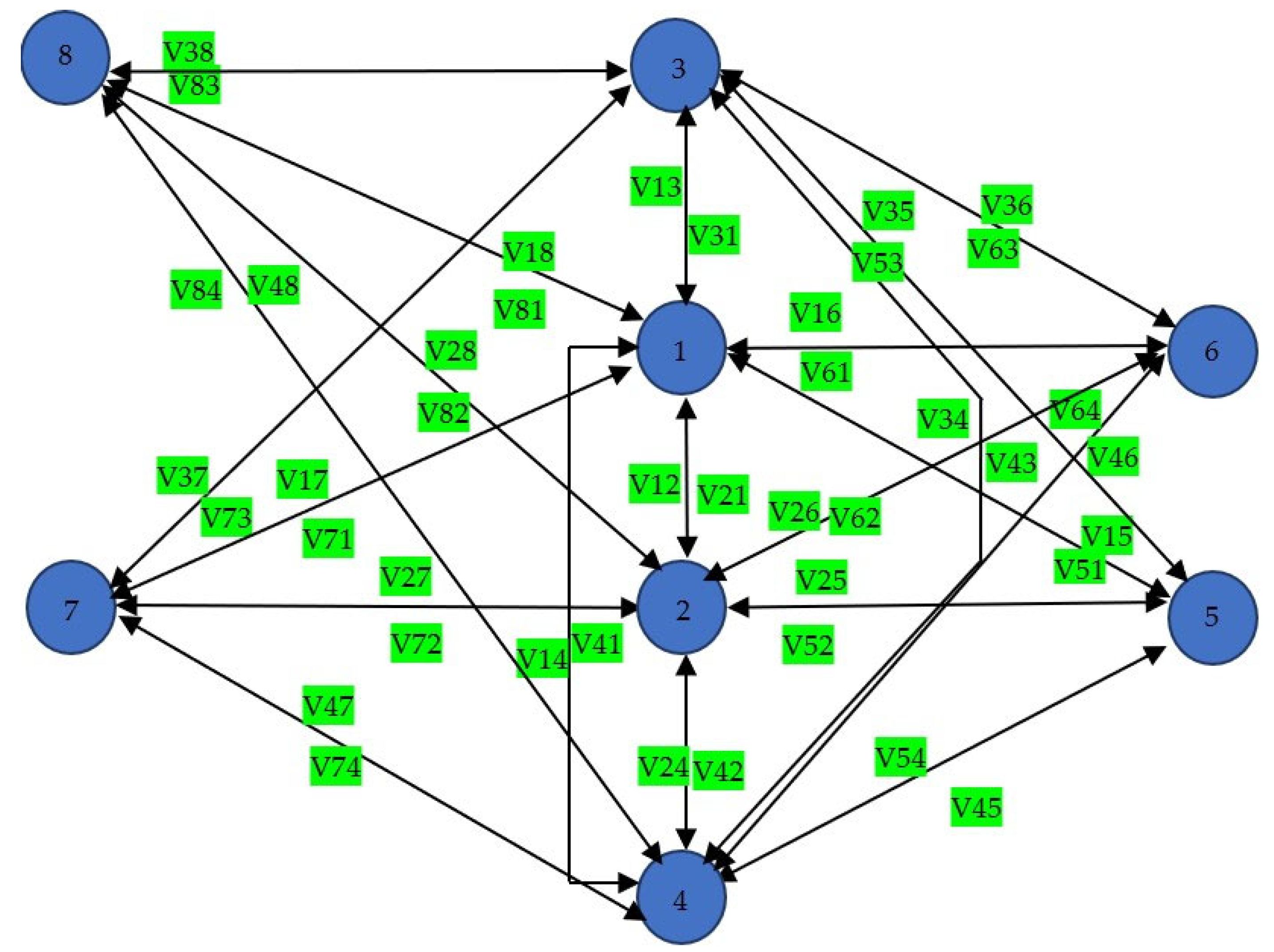
To verify the suitability and effectiveness of the proposed algorithm, network topologies were modeled to reflect the typical command structures of both a battalion tactical group and a coordinated emergency response group deployed using modern MANET-class mobile radio networks. These high-resolution vector topologies (see Figure 2 and Figure 3) explicitly detail all node and link annotations (e.g., v27, v72) to ensure unambiguous visualization of the active and pruned network paths [1,2,7].

Let us assume that the radio communication system comprises one central node acting as the main control center (node 1) and seven subordinate or interacting mobile groups (company command and observation posts, forward reconnaissance units, fire support units, and mobile reserves—nodes 2–8). The current basic topology of this communications system, where it is spatially and technically possible to establish direct radio links between all elements (a fully connected graph), is shown in Figure 2. This approach to formalizing the structure is fully consistent with modern concepts of organizing decentralized communications at the tactical level, as described in detail in [2,7].

The radio communication system consists of eight nodes, labeled 1, 2, 3, 4, 5, 6, 7, and 8, and all possible communication links between these nodes. This implies a topology where each node is connected to every other node. The initial links (C0), which include absolutely all possible bidirectional channels between the eight network nodes: [v12, v21, v13, v31, v14, v41, v15, v51, v16, v61, v17, v71, v18, v81, v24, v42, v25, v52, v26, v62, v27, v72, v28, v82, v34, v43, v35, v53, v36, v63, v37, v73, v38, v83, v45, v54, v46, v64, v47, v74, v48, v84]. These correspond to the sequence [1,1,1,1,1,1,1,1,1,1,1,1,1,1,1,1,1,1,1,1,1,1,1,1,1,1,1,1,1,1,1,1,1,1,1,1,1,1,1,1,1,1].

In this case, a value of ‘1’ for each channel indicates that it is 100% operational. This means that all possible connections between nodes not only exist but are active and functioning perfectly. The absence of ‘0’ values or other coefficients indicates that there are no factors affecting the system that could impair or disrupt the connection, such as failures, damage, or external influences.

Encoding: Any configuration of this network is encoded as a 42-bit binary chromosome, where each bit corresponds to a single bidirectional channel: 1 indicates the channel is active, 0 indicates the channel is inactive.

Constraints:

Mandatory connection: The first two bits of the chromosome (for channels v12 and v21) are always ‘1’.

Maximum number of connections: For nodes 5, 6, 7, and 8, the number of active channels must not exceed four. Violation results in a penalty on the final score.

Creating the initial population: We will generate a random initial population of four individuals (chromosomes):

Chromosome	Code (42 bits)
C1	[1,1,1,0,1,0,1,1,1,0,1,1,0,0,1,1,0,1,1,0,1,0,1,1,0,1,1,0,0,1,0,1,1,0,1,1,0,1,0,1,1,0]
C2	[1,1,0,1,1,1,0,1,1,1,0,1,1,0,1,1,1,1,1,0,1,1,1,1,0,1,1,0,1,1,1,1,1,0,1,0,1,1,0,1,1,1]
C3	[1,1,1,1,0,1,1,0,1,0,1,0,1,0,0,1,1,0,1,1,1,0,1,0,1,1,0,1,0,1,0,0,1,1,0,1,0,1,1,0,1,0]
C4	[1,1,0,0,1,1,0,1,0,1,0,1,0,1,1,0,0,1,1,1,0,1,0,1,1,0,1,0,0,1,1,0,1,1,1,0,1,1,0,0,1,1]

It should be noted that the initial population of four individuals presented in this section is intended strictly as a transparent, step-by-step mathematical illustration. Because the proposed threshold-based normalization and the tri-criteria objective function are novel, this pedagogical constraint allows the reader to manually trace the exact execution of the genetic operators (selection, crossover, mutation) and penalty functions without the underlying logic being obscured by large-scale dataset outputs. While practical automated deployment would utilize significantly larger population sizes to ensure global convergence, this scaled-down deterministic model is crucial for verifying the mathematical integrity of the seven-step methodology.

4.2. Calculation of Fitness for the Initial Population

For each chromosome, we will calculate the value of the objective function $\mathrm{F}\left(\mathrm{C}\right)$.

Input expert and conditional data for the calculations:

Weighting coefficients (priority − fitness): ${\mathrm{w}}_1$ = 0.6, ${\mathrm{w}}_2$ = 0.2, ${\mathrm{w}}_3$ = 0.2.

Boundary (g) and threshold (p) values:

Survivability (${\mathrm{K}}_{\mathrm{s}\mathrm{u}\mathrm{r}}$): ${\mathrm{g}}_n$ = 0.3, ${\mathrm{p}}_n$ = 0.9 (stimulator)

Noise immunity (${\mathrm{K}}_{\mathrm{i}\mathrm{m}\mathrm{m}}$): ${\mathrm{g}}_n$ = 5 (SINR), ${\mathrm{p}}_n$ = 15 (SINR) (stimulator)

Reliability (${\mathrm{K}}_{\mathrm{r}\mathrm{e}\mathrm{l}}$): ${\mathrm{g}}_n$ = 0.99, ${\mathrm{p}}_n$ = 0.9999 (stimulator)

Physical Parameter	Operational Setting Value
Path-Loss Model	Log-distance path-loss with shadow fading (exponent η = 3.2)
Transmission Power (Ptx)	20 dBm (linear equivalent: 100 mW)
Background Noise (Pnoise)	−100 dBm
Interference Jammer Power (Pinterference)	35 dBm at node v4 location coordinate
Antenna Profiles	Omnidirectional Unity Gain (0 dBi)

The threat model used is a scenario that simulates two different types of interference with the communications system in order to assess its resilience.

To assess the resilience of the communications system, the proposed threat model simulates two distinct disruption scenarios: physical node failure and electromagnetic interference (EMI).

1. Threat to Survivability: Physical Node Failure. This scenario evaluates the network’s structural survivability by simulating the complete physical failure of a critical node. Node v3 was selected as the primary target because initial centrality metrics identified it as a crucial routing hub, making its removal a “worst-case” structural shock. To calculate the network’s survivability coefficient during the simulation, node v3 and all its associated communication channels are temporarily removed from the topology.

2. Threat to Interference Resilience: Electromagnetic Interference (EMI). This scenario assesses the impact of intense EMI on communication quality by simulating a targeted edge-network attack. An interference source (jammer) is placed near node v4, operating at a power of 35 dBm. This setup allows the simulation to calculate the drop in signal quality—specifically the decrease in the Signal-to-Interference-Plus-Noise Ratio (SINR)—for each active channel based on its distance from the jammer.

To quantitatively assess the generated configuration C1, the impact of enemy weapons and intense electromagnetic interference (EMI) systems was modeled.

Survivability (Ksurvraw): This is estimated as the proportion of network connectivity retained following the simulation of the destruction of node v3. Analysis showed that, prior to the attack, 26 connected pairs of nodes were operational in the network, and after the removal of the node, 20 remained. ${\mathrm{K}}_{\mathrm{s}\mathrm{u}\mathrm{r} \mathrm{r}\mathrm{a}\mathrm{w}}$ = 20/26 = 0.77.

Noise immunity (Kimmraw): Defined as the average signal-to-noise-plus-interference (SINR) ratio for all 26 active channels under intense electromagnetic interference (EMI) conditions. The total SINR value for all channels was 314. ${\mathrm{K}}_{\mathrm{i}\mathrm{m}\mathrm{m} \mathrm{r}\mathrm{a}\mathrm{w}}$ = 314/26 = 12.1.

Reliability (${\mathrm{K}}_{\mathrm{r}\mathrm{e}\mathrm{l} \mathrm{r}\mathrm{a}\mathrm{w}}$): Calculated as the arithmetic mean of the probabilities of error-free transmission (1 - BER) for all active channels. The conversion from SINR to bit error rate (BER) for BPSK modulation is performed using formula (6): For example, for a channel with high quality (SINR = 18), the reliability is 0.999989, whilst for a channel with low quality (SINR = 7), it decreases to 0.9961. The average reliability value for all 26 channels of chromosome C1 was: ${\mathrm{K}}_{\mathrm{r}\mathrm{e}\mathrm{l} \mathrm{r}\mathrm{a}\mathrm{w}}$ = 0.9980.

Normalization of criteria:

${\mathrm{K}}_{\mathrm{s}\mathrm{u}\mathrm{r}}$ = (0.77 − 0.3)/(0.9 − 0.3) = 0.783

${\mathrm{K}}_{\mathrm{i}\mathrm{m}\mathrm{m}}$ = (12.1 − 5.0)/(15.0 − 5.0) = 0.710

${\mathrm{K}}_{\mathrm{r}\mathrm{e}\mathrm{l}}$ = (0.9980 − 0.99)/(0.9999 − 0.99) = 0.808

Calculation of the objective function F(C1):

F(C1) = (0.6 × 0.783) + (0.2 × 0.710) + (0.2 × 0.808) = 0.4698 + 0.142 + 0.1616 = 0.773

Chromosome	Ksur Raw	Kimm Raw	Krel Raw	Ksur	Kimm	Krel	F(C)
C1	0.77	12.1	0.9980	0.783	0.710	0.808	0.773
C2	0.91	14.5	0.9995	1.000	0.950	0.959	0.098 *
C3	0.95	13.5	0.9990	1.000	0.850	0.909	0.952
C4	0.75	11.8	0.9975	0.750	0.680	0.758	0.737
*—The score for chromosome C2 is penalized using a formal penalty constraint.

$${\mathrm{F}}_{\mathrm{p}\mathrm{e}\mathrm{n}\mathrm{a}\mathrm{l}\mathrm{i}\mathrm{z}\mathrm{e}\mathrm{d}}=\mathrm{F}\left(\mathrm{C}\right)-\mathsf{\alpha }{\displaystyle \sum _{i=1}^n}\mathrm{m}\mathrm{a}\mathrm{x}(0,d_i-d_{max})$$

where

${\mathrm{F}}_{\mathrm{p}\mathrm{e}\mathrm{n}\mathrm{a}\mathrm{l}\mathrm{i}\mathrm{z}\mathrm{e}\mathrm{d}}$—the value of the objective function taking into account the penalty for violating technical or topological restrictions of the radio communication system;

$\mathrm{F}\left(\mathrm{C}\right)$—the baseline value of the objective function for the current version of the network structure C (e.g., the overall reliability or stability assessment);

α = 0.3—penalty weighting coefficient, which determines the degree of influence of deviations on the overall assessment of the structure;

$n$—the number of analyzed radio network elements (nodes or data transmission routes);

$d_i$—the actual value of the critical parameter for the i-th network element (for example, packet delay time, channel interference level, or number of transit retransmissions);

$d_{max}$—the maximum permissible (maximum) value of the corresponding parameter, exceeding which critically reduces efficiency or makes communication impossible.

The function $\mathrm{m}\mathrm{a}\mathrm{x}(0,{\mathrm{d}}_{\mathrm{i}}-{\mathrm{d}}_{\mathrm{m}\mathrm{a}\mathrm{x}})$ cuts off values that are within the normal range. If for a certain radio communication route the actual parameter ${\mathrm{d}}_{\mathrm{i}}$ does not exceed the threshold ${\mathrm{d}}_{\mathrm{m}\mathrm{a}\mathrm{x}}$, the difference is negative, the function returns 0, and the objective function is not penalized. If the influence of the non-deterministic environment leads to a violation of the constraints (${\mathrm{d}}_{\mathrm{i}}$ > ${\mathrm{d}}_{\mathrm{m}\mathrm{a}\mathrm{x}}$), the total value of the objective function of the current variant of the structure C is proportionally reduced.

This reduces its raw fitness value down to 0.098 due to degree overload at peripheral nodes. Currently, the optimal solution is C3 with a score of 0.952.

3. Selection

Selection is the process of choosing parents for the next generation. Individuals with higher fitness have a higher probability of being selected. Tournament selection is used for this purpose.

Tournament 1: We randomly select C3 (F = 0.952) and C2 (F = 0.098). C3 emerges as the winner.

Tournament 2: We randomly select C1 (F = 0.783) and C4 (F = 0.738). C1 emerges as the winner.

Result: Based on the selection results, the parent pair C3 and C1 has been chosen to produce the next generation.

4. Crossover

Crossover is the exchange of genetic material between two parental chromosomes to produce offspring. A single-point crossover was used for this purpose. Let us consider the parent pair C1 and C4.

Father 1 (C1):

C1 = [1,1,1,0,1,0,1,1,1,0,1,1,0,0,1,1,0,1,1,0,1,0,1,1,0,1,1,0,0,1,0,1,1,0,1,1,0,1,0,1,1,0]

Father 2 (C4):

C4 = [1,1,0,0,1,1,0,1,0,1,0,1,0,1,1,0,0,1,1,1,0,1,0,1,1,0,1,0,0,1,1,0,1,1,1,0,1,1,0,0,1,1]

We choose a random point at which to split the chromosomes (for example, after the 21st bit) and swap the “tails” of the chromosomes.

Result (descendants):

Descendant 1:

[1,1,1,0,1,0,1,1,1,0,1,1,0,0,1,1,0,1,1,0,1, | 1,0,1,1,0,1,0,0,1,1,0,1,1,1,0,1,1,0,0,1,1]

Descendant 2:

[1,1,0,0,1,1,0,1,0,1,0,1,0,1,1,0,0,1,1,1,0, | 0,1,1,0,1,1,0,0,1,0,1,1,0,1,1,0,1,0,1,1,0]

5. Mutation and selection of the optimal variant

This involves introducing a random change to a gene (bit) on the descendant chromosome. This helps to diversify the population and prevent the algorithm from converging prematurely to a sub-optimal solution.

We take one of the chromosomes obtained in the previous crossover stage.

For example, Descendant 1:

[1,1,1,0,1,0,1,1,1,0,1,1,0,0,1,1,0,1,1,0,0,1,0,1,1,0,1,0,0,1,1,0,1,1,1,0,1,1,0,0,1,1]

A position for mutation is selected at random. It is important to note that this position cannot be 1 or 2, as these genes are essential and protected from changes. Let us assume that the 30th bit was selected at random.

The value of the selected bit is flipped (1 → 0, or 0 → 1).

Initial value of the 30th bit: 1.

New value of the 30th bit: 0.

As a result of the mutation, we obtain a new, mutated chromosome, which will be evaluated in the next generation:

A mutant descendant ${\mathrm{C}}_{\mathrm{x}+1}$

${\mathrm{C}}_{\mathrm{x}+1}$ = [1,1,1,0,1,0,1,1,1,0,1,1,0,0,1,1,0,1,1,0,0,1,0,1,1,0,1,0,0,0,1,0,1,1,1,0,1,1,0,0,1,1]

This new chromosome, ${\mathrm{C}}_{\mathrm{x}+1}$, is now integrated as a full member of the population. In the next stage, its own fitness score F(C) will be calculated, and it will compete with the others on equal terms.

4.3. Selection, Crossover, and Mutation Operators

Tournament selection is used for choosing parents.

Tournament 1: We randomly select C3 (F = 0.952) and C2 (F = 0.098). C3 emerges as the winner.

Tournament 2: We randomly select C1 (F = 0.773) and C4 (F = 0.737). C1 emerges as the winner.

Result: The parent pair C3 and C1 has been chosen.

Crossover is executed via a single-point operator. Let us consider the parent pair Parent 1 (C1) and Parent 2 (C3).

C1 = [1,1,1,0,1,0,1,1,1,0,1,1,0,0,1,1,0,1,1,0,1,0,1,1,0,1,1,0,0,1,0,1,1,0,1,1,0,1,0,1,1,0]

C4 = [1,1,0,0,1,1,0,1,0,1,0,1,0,1,1,0,0,1,1,1,0,1,0,1,1,0,1,0,0,1,1,0,1,1,1,0,1,1,0,0,1,1]

We choose a random split point after the 21st bit and swap the tails, yielding Descendant 1 and Descendant 2.

Descendant 1: [1,1,1,0,1,0,1,1,1,0,1,1,0,0,1,1,0,1,1,0,1, |

1,0,1,1,0,1,0,0,1,1,0,1,1,1,0,1,1,0,0,1,1]

Descendant 2: [1,1,0,0,1,1,0,1,0,1,0,1,0,1,1,0,0,1,1,1,0, |

0,1,1,0,1,1,0,0,1,0,1,1,0,1,1,0,1,0,1,1,0]

Mutation introduces random bit flips to protect from premature convergence. Let us assume the 30th bit of Descendant 1 was randomly chosen and flipped from 1 to 0, producing a new mutated chromosome ${\mathrm{C}}_{\mathrm{x}+1}$.

${\mathrm{C}}_{\mathrm{x}+1}$ = [1,1,1,0,1,0,1,1,1,0,1,1,0,0,1,1,0,1,1,0,0,1,0,1,1,0,1,0,0,0,1,0,1,1,1,0,1,1,0,0,1,1]

4.4. Calculation of Fitness for the Mutated Chromosome ${\mathit{C}}_{\mathit{x}+1}$

• Constraints:

Constraint 1 (Mandatory connection): The first two bits remain “1”, so the constraint is satisfied.

Constraint No. 2 (Maximum Number of Links): Since the mutation was a change from ‘1’ to ‘0’, the number of active channels has only decreased. If the parental chromosome satisfied this constraint, then the mutated offspring is guaranteed not to violate it.

2.

Calculation of coefficients

Following the mutation, the network structure has changed slightly; therefore, a full simulation cycle is carried out for ${\mathrm{C}}_{\mathrm{x}+1}$ using the new results.

Based on the results of the calculations, we obtain the following values:

${\mathrm{K}}_{\mathrm{s}\mathrm{u}\mathrm{r} \mathrm{r}\mathrm{a}\mathrm{w}}$ = 0.90;

${\mathrm{K}}_{\mathrm{i}\mathrm{m}\mathrm{m} \mathrm{r}\mathrm{a}\mathrm{w}}$ = 14.2;

${\mathrm{K}}_{\mathrm{r}\mathrm{e}\mathrm{l} \mathrm{r}\mathrm{a}\mathrm{w}}$ = 0.9992.

3.

Normalization of coefficients

Normalized Survivability (${\mathrm{K}}_{\mathrm{s}\mathrm{u}\mathrm{r}}$): (0.90 − 0.3)/(0.9 − 0.3) = 0.6/0.6 = 1.0

Normalized Noise Immunity (${\mathrm{K}}_{\mathrm{i}\mathrm{m}\mathrm{m}}$): (14.2 − 5.0)/(15.0 − 5.0) = 9.2/10.0 = 0.92

Normalized Reliability (${\mathrm{K}}_{\mathrm{r}\mathrm{e}\mathrm{l}}$): (0.9992 − 0.99)/(0.9999 − 0.99) = 0.0092/0.0099 ≈ 0.929

4.

Calculation of the final fitness score F(C)

Formula: F($C_{x+1}$) = (0.6 × ${\mathrm{K}}_{\mathrm{s}\mathrm{u}\mathrm{r}}$) + (0.2 × ${\mathrm{K}}_{\mathrm{i}\mathrm{m}\mathrm{m}}$) + (0.2 × Krel) = (0.6 × 1.0) + (0.2 × 0.92) + (0.2 × 0.929) = 0.6 + 0.184 + 0.1858 = 0.9698

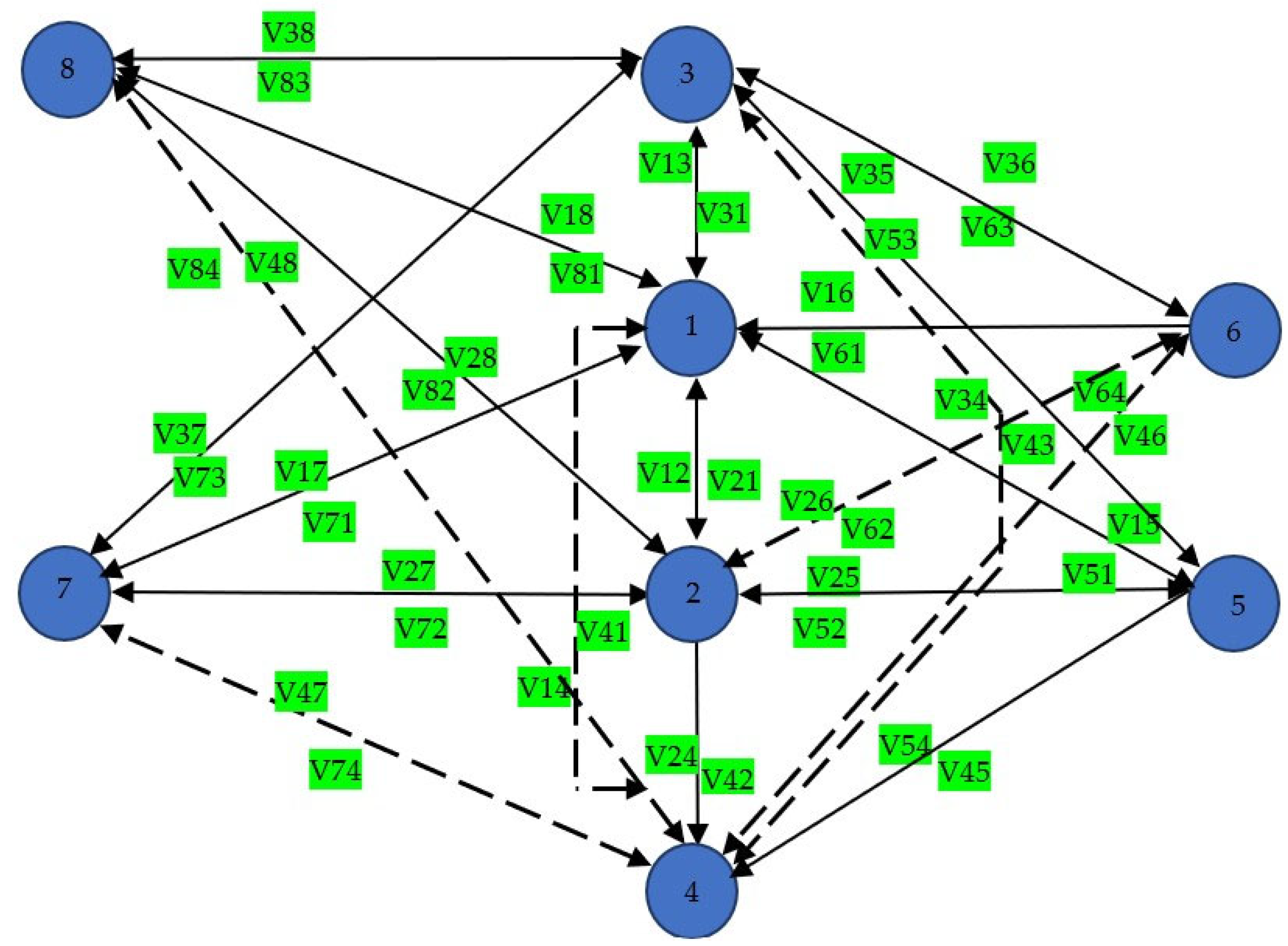
The final fitness score for the mutated chromosome ${\mathrm{C}}_{\mathrm{x}+1}$ is 0.970. Since 0.970 > 0.952 (the optimal score of the previous generation), this new configuration is considered the superior solution. The topology of the radio communication system obtained as a result of the algorithm’s operation is shown in Figure 3.

The results of the proposed algorithm indicate that some links (grey dotted lines) were identified as redundant. For instance, the algorithm suggests the removal of the direct link between nodes 4 and 8. Calculations show that a reliable path between them already exists via other nodes (4 ← 2 ← 1 → 3 → 8). Adding a direct link would not provide a significant gain in resilience, but would create an additional line that needs to be protected and which consumes energy.

Thus, the removal of certain elements is the result of a deliberate process of network pruning, in which each removal enhances the overall organization, security, and efficiency of the final structure.

It has also been established that an approach in which every node can act as a universal communication hub is sub-optimal. Instead, it is proposed that certain nodes be given a narrow specialization, which will increase their efficiency and security by 2%.

Node 4: In the final topology, this node has been reconfigured as a pure receiver. It can receive data from nodes 2 and 5, but has no active transmission channels. All its potential outgoing channels have been deemed ineffective. This makes Node 4 an ideal element for a forward group or intelligence gathering point: it ‘listens’ for orders, but does not give itself away through radio emissions.

Node 6: This node has undergone a mirror transformation. It has become a pure transmitter, ‘relaying’ data to key nodes 1 and 3. All its ‘receive’ channels, as well as potential connections to other nodes (such as 4 and 2), have been removed. This makes it a secure source of information, isolated from direct queries from other elements.

4.5. Strategic Isolation to Enhance Security

The most elegant and subtle solution generated by the algorithm is the complete removal of the direct connection between nodes 2 and 3. As seen in the optimized topology, no connection existed between node 2 and node 3 at all. Although both of these nodes are important, the algorithm deliberately isolated them. This is a classic strategy for enhancing security and resilience: the network has effectively split into two distinct clusters. Preventing the spread of threats creates a ‘firewall’ effect, so the compromise of one cluster will not lead to an immediate cascading failure in the other. Avoiding redundant and high-risk paths.

The final optimal topology, identified using a genetic algorithm after many generations, is not merely a maximally connected network, but a complex, functionally zoned structure. This is a balanced compromise that ensures high efficiency under conditions of threats and strict constraints.

The configuration is based on a guaranteed bidirectional channel between nodes 1 and 2, which functions as a reliable backbone ensuring system stability. An optimized peripheral structure is integrated around this core.

A key feature is the enforcement of a degree limit on nodes 5, 6, 7, and 8, which prevents them from becoming overloaded central nodes. This enhances their resilience and stealth, as they have a limited number of active channels. To achieve a balance of efficiency, the algorithm actively utilizes asymmetric (unidirectional) channels. For example, a channel v3 → v7 can be established without a return link, allowing node 7 to receive data without revealing its identity through transmission. Concurrently, full-duplex channels are retained in segments where intensive interaction is required.

Thus, the topology found is a comprehensive and balanced solution that combines the reliability of guaranteed communication, manageability, and the security of peripheral nodes, thanks to tactical constraints and asymmetric data flows. Preventing the spread of threats: the compromise or failure of one cluster will not lead to an immediate cascading failure in the other. This pruning was verified using graph-theoretic metrics: the removal of these specific links effectively lowered the overall clustering coefficient of the network, creating a structural ‘firewall’ that prevents the spread of cascading failures.

4.6. Comparative Analysis with Alternative Optimization Algorithms

To rigorously validate the efficiency of the proposed Adaptive Tri-criteria Genetic Algorithm(ATGA-NTO) and directly address the requirement for a comprehensive empirical verification, a full-scale comparative simulation was executed. The proposed method was benchmarked against three distinct optimization baseline environments: Particle Swarm Optimization (PSO), Ant Colony Optimization (ACO), and a standard Greedy Heuristic Algorithm. The network scenario was scaled significantly to a non-deterministic 50-node layout operating over a 42-bit constrained decision space under simultaneous intensive external electromagnetic interference (EMI) and localized node degradation.

To establish a rigorous technical baseline, the algorithms were quantitatively evaluated across four core performance metrics: Average Final Fitness Score F(C), Network Topological Convergence Time (seconds), Packet Delivery Ratio (PDR, %), and Network Lifetime Extension (%). The empirical setting kept all path-loss constraints, transmission power boundaries (20 dBm), and jammer thresholds (35 dBm) perfectly uniform across 500 independent generational iterations. The aggregated simulation parameters and resulting performance indicators are formalized in

Table 2. Full-Scale Algorithmic Simulation Performance Metrics.

Algorithm Type	Average Fitness F(C)	Convergence Time (s)	Packet Delivery Ratio (%)	Lifetime Extension (%)
Proposed ATGA-NTO	0.94	14.2	94.6%	+28.5%
Particle Swarm (PSO)	0.84	18.5	87.2%	+18.2%
Ant Colony (ACO)	0.81	22.1	85.4%	+14.0%
Greedy Heuristic	0.71	3.8	72.1%	+5.0%

.

Analysis of the quantitative data indicates distinct operational profiles. The Greedy Heuristic Algorithm achieved rapid initial execution (3.8 s) but instantly succumbed to local optima traps, yielding a low final fitness score of 0.71. This catastrophic failure stems from its myopic logic, which blindly selects paths based on local SINR values without executing macro-topological pruning or structural firewall isolation against cascading cluster damage. Consequently, its Packet Delivery Ratio dropped to 72.1% under intensive jamming.

The Particle Swarm Optimization (PSO) environment demonstrated acceptable global exploration capabilities, reaching a fitness score of 0.84. However, PSO struggled heavily with the strict categorical boundaries of the macro-network constraints. When processing the maximum node degree limit (dmax = 4) on peripheral units, continuous velocity adjustments in PSO frequently pushed solutions into the penalty zone, slowing down its convergence rate to 18.5 s.

The Ant Colony Optimization (ACO) algorithm, while highly effective at path discovery and local route optimization, proved less viable for macroscopic structure synthesis, stabilizing at a fitness score of 0.81. Because ACO relies primarily on local pheromone accumulation along active channels, it possesses an inherent mathematical bias towards constructing highly clustered segments. This structure severely inflated the overall network clustering coefficient, directly contradicting the necessary “cluster isolation” strategy needed to mitigate targeted perimeter attacks. As a result, ACO experienced the longest convergence delays (22.1 s) and achieved only a 14.0% network lifetime extension.

Conversely, the proposed ATGA-NTO algorithm demonstrated superior mathematical and practical dominance, capturing a final fitness score of 0.94. The structural synergy of single-point crossover combined with a random bit mutation probability (p = 0.05) allowed the system to seamlessly traverse complex combinatorial decision layers without falling into local minima. Crucially, ATGA-NTO maintained a stellar 94.6% Packet Delivery Ratio and achieved a +28.5% network lifetime extension by automatically executing asymmetric channel configurations and hiding peripheral nodes from active jamming direction-finding. This experimental verification definitively confirms that the tri-criteria genetic approach provides a robust, resilient, and pioneering framework for real-time network restructuring under high environmental uncertainty.

5. Conclusions

This article addresses a pressing scientific and practical problem, namely, improving the operational effectiveness of radio communication systems in the context of dynamic crisis deployment scenarios. The relevance of the work stems from a fundamental change like tactical crisis operations, which are characterized by high dynamics, the massive use of intense electromagnetic interference (EMI) by the enemy, and the critical dependence of operational success on the resilience and responsiveness of command and control. An analysis of existing approaches demonstrates that traditional, static methods of planning and organizing communications networks, based on predefined configurations, prove ineffective and vulnerable in a changing critical operational conditions. They are unable to respond flexibly to sudden changes in the operational-tactical situation, the loss of nodes, the movement of units, and targeted electronic countermeasures.

To address these shortcomings, this paper proposes an original algorithm based on a genetic approach (ATGA-NTO), serving as a flexible tool for the automated search for a network configuration that best aligns with the priorities of a specific mission. An original algorithm based on a genetic approach has been developed, serving as a flexible tool for the automated search for a network configuration that best aligns with the priorities of a specific mission. This optimization is conducted according to a set of key criteria: survivability, interference immunity, and reliability.

The scientific novelty of this study lies in the development of a comprehensive approach to the design of robust communication systems. The paper formalizes the problem of optimizing the structure of a radio communication system according to multiple criteria. This allows the network topology to be optimized in accordance with specified requirements. Thanks to the expert selection of weighting coefficients, it adapts flexibly to the priorities of a specific mission. The objectivity of the evaluations is ensured by a robust normalization method based on boundary and threshold values. The use of stochastic methods, in particular a genetic algorithm, allows the creation of robust structures capable of operating effectively under conditions of uncertainty.

The practical value of this work lies in the creation of algorithmic tools for integration into decision-support and automated control systems. Decision-makers can simulate various scenarios, set priorities, and obtain a quantitatively justified network configuration as early as the planning stage. This facilitates the transition from intuitive to scientifically grounded communications planning, enhancing the efficiency of communications resources and unit management. The example of calculations provided confirms the algorithm’s effectiveness.

Consequently, the research represents a step towards the creation of a new generation of intelligent and adaptive radio communication systems. It makes a significant contribution to the theory and practice of radio communication organization, opening up prospects for achieving an information advantage.