Per-Flow Throughput of a FIFO Buffer

Abstract

FIFO buffers are widely employed in networking devices to store packets prior to transmission. Their impact on aggregate traffic has been extensively studied and is well documented in the literature. In contrast, significantly less attention has been allocated to the impact of FIFO buffers on individual flows contributing to the aggregate traffic. In this paper, the throughput of each flow traversing a FIFO buffer supplied with complex traffic composed of numerous flows, potentially exhibiting heterogeneous statistical properties, is investigated. A full queuing model of a FIFO buffer fed by many flows with different characteristics is considered first. This model is very precise with respect to each flow, but cannot be solved in practice. Then, a simplification of the full model based on a limiting theorem is proposed. For the simplified model, exact formulae for throughput and loss ratio of each participating flow are derived. In numerical examples, the throughput of flows of diverse types in scenarios with various buffer sizes, buffer loads, and transmission time distributions is calculated. It is also examined, how these factors influence per-flow throughput. Finally, it is demonstrated that in typical scenarios, the results of the simplified model differ by only a few percent from those obtained through simulations of the full, precise model.

1. Introduction

From the very beginning of packet-switching networks, it was understood that buffers for packets are absolutely necessary to achieve reasonably low loss ratios and high network throughput.

As a consequence, queueing theory for packets in buffers began to be widely used to evaluate the performance of packet networks, and one of the founding fathers of the Internet, Leonard Kleinrock, is also an expert in queueing theory. Since the first packet transmission conducted in ARPANET by Kleinrock’s student, many papers have been devoted to modeling queues of packets in buffers in order to predict queueing delay, delay jitter, throughput, and packet loss induced by the buffers.

However, a great majority of these papers and monographs have been committed to the analysis of the impact that a buffer has on aggregated traffic, differentiating among separate flows. Namely, the obtained formulae provide the delay, loss probability, etc., of an average packet belonging to a random flow among all the flows multiplexed in the buffer.

On the other hand, it is easy to show, using simulations or network measurements, that packet flows with different statistical properties may behave very differently when traversing a common buffer. For instance, in simulations of [1], it can be seen that per-flow loss ratios may differ from each other by an order of magnitude, no matter that they share the same rate and differ only in the specific interarrival time distribution. This is a drastic difference for flows that, at first glance, seem to be similar (same rate).

The distinction between flows with separate statistical behavior is not only theoretical but also has strong practical motivation. Traffic in contemporary IP networks is highly inhomogeneous. It often consists of a large number of flows of distinct types, such as web browsing, teleconferencing, gaming, and TV streaming. All these flows may differ greatly from each other in a statistical sense.

A comparable circumstance may be encountered in sensor networks. Flows of packets from various sensors incoming to aggregation points may have very different statistical properties due to the various types of sensors and the data streams they produce.

Therefore, the primary aim of this paper is to derive the throughput and loss ratio of every flow traversing a common FIFO buffer, assuming the buffer is loaded by complex traffic consisting of many flows, possibly with totally different statistical properties.

This goal is achieved in three steps. First, a full, precise model of traffic consisting of N flows is used. In this model, every flow can be modeled separately with high precision, including not only interarrival time moments but also the shape of the distribution. Unfortunately, as will be argued, this model cannot be solved in practice. Therefore, in the second step, a simplification of the full model is used. In this simplification, one particular flow of interest is modeled precisely, while all the remaining flows are combined into simplified background traffic. Such an approach is justified by one of the limiting theorems of probability theory.

In the third step, an exact, explicit solution of the simplified model is found, i.e., formulae for throughput and loss ratio for the flow of interest are derived (Theorem 1). To fully solve a system with N flows, this simplification procedure has to be performed N times, i.e., Theorem 1 has to be applied N times. Specifically, a model with a precise characterization of flow number 1 and simplified background traffic consisting of flows 2–N has to be solved first. Then, a model with a precise characterization of flow number 2 and simplified background traffic consisting of flows 1 and 3–N has to be solved, and so on. By doing so, N throughput values and N loss ratios can be obtained.

Naturally, the results obtained via the simplified model are only approximations of the precise values offered by the full model. To evaluate the errors of these approximations, several numerical experiments were performed. In these experiments, the reference values were obtained using simulations of the full model with large numbers of packets traversing the FIFO buffer.

As will be seen, the relative error of per-flow throughput prediction was about 8% in some very demanding cases, i.e., with a very small number of flows, highly diversified flow characteristics (rates and coefficients of variation), a very small buffer, high system load, and high variance of packet transmission time. In other, less extreme scenarios, the results predicted by Theorem 1 were much better, often offering an error below 1%.

Summarizing, the principal contributions of this paper are:

• The derivation of an exact analytical solution for per-flow throughput and loss ratio in a simplified model of a FIFO buffer fed by multi-flow traffic (Theorem 1);
• A numerical validation of the accuracy of the simplified model across a range of scenarios characterized by heterogeneous flow statistics, varying buffer sizes, system loads, and transmission time distributions;
• A discussion of the impact of these parameters on per-flow throughput.

The article continues as follows. In Section 2, prior research on multi-flow and single-flow queueing models related to this study is reviewed. In Section 3, the full, precise multi-flow model of a FIFO buffer is presented, along with arguments showing that its numerical solution is, in practice, far beyond reach. Then, a simplified, analytically and numerically tractable model is described in Section 4.

In Section 5, an exact, explicit solution of the simplified model is obtained (Theorem 1). Specifically, formulae for the per-flow throughput and loss ratio are proved. In Section 6, the results of numerical experiments are presented and discussed. Specifically, in various scenarios, the results calculated using Theorem 1 are compared with those obtained via simulation of the full model. Flows with various rates and interarrival time variability are considered, together with different buffer sizes, system loads, and transmission times.

Finally, concluding remarks are offered in Section 7. These include a discussion of the limitations of the simplified model and ideas for subsequent work.

2. Prior Research

There is a body of literature on experimental measurements of throughput and losses [2,3,4,5,6,7], with no mathematical modeling of these characteristics.

Mathematical modeling of FIFO buffer’s throughput and losses, for basic models of aggregate traffic, is presented in classic queueing monographs–see, e.g., [8,9] and the references therein. More advanced models, incorporating autocorrelation, batch arrivals, or special loss characteristics, are studied in [10,11,12,13,14,15], but again only at the level of aggregate traffic.

Studies of multi-flow queueing models began with the assumption that all flows are Poisson [16,17,18,19]. Unfortunately, when all flows are Poisson, all of them share a common loss ratio equal to the aggregate loss ratio. This is in blatant contradiction with networking reality, as demonstrated in [1]. Namely, when separate flows are non-Poisson–as commonly occurs in practice–they may have loss ratios that differ by an order of magnitude.

Multi-flow queueing models in which each flow has a separate, general interarrival time distribution were investigated in [20,21,22,23,24]. However, all the models in [20,21,22,23,24] assume infinite buffering space. Hence, none of them accounts for packet losses and throughput degradation caused by buffer overflow.

There are also a few studies of multi-flow queueing models in which the transmission time is constant [25,26,27,28]. Constant packet/cell sizes are used in ATM networks, which were more popular in the past. In most contemporary networks, packets can have variable sizes, which results in variable service (transmission) times. From elementary queueing theory, it is known that variability of service time may strongly affect queueing performance.

Summarizing, there is no published multi-flow model with:

• An arbitrary interarrival time distribution for each flow;
• An arbitrary transmission time distribution;
• A FIFO buffer with finite capacity.

Each of these features may have a significant impact on per-flow throughput. Therefore, incorporating all of them into a single mathematical model is essential.

The model presented in this paper addresses all the points listed above and enables the calculation of the throughput and loss ratio for each individual flow.

The method of analysis used here is similar to the method presented in [29]. However, a single-flow model is considered there, and the paper focuses on the buffer occupancy, whereas this study focuses on per-flow throughput and losses.

A recap of the related research is presented in

Table 1. Related research.

Experimental measurements of throughput and losses	[2,3,4,5,6,7]
Models with aggregate traffic, no distinction between flows	vast literature, e.g., [8,9,10,11,12,13,14,15,29]
Multi-flow models with infinite buffer, i.e., no losses, no reduction in throughput by losses	[20,21,22,23,24]
Multi-flow models with all flows Poisson and common loss ratio	[16,17,18,19]
Multi-flow models with constant service times	[25,26,27,28]
Multi-flow model with an advanced model of each flow, general service times, a finite buffer, diversified per-flow throughput and loss ratio	this work

.

3. Full Multi-Flow Model

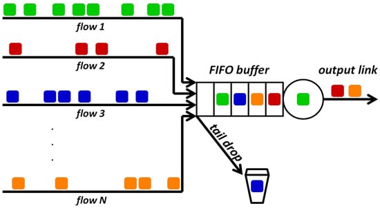
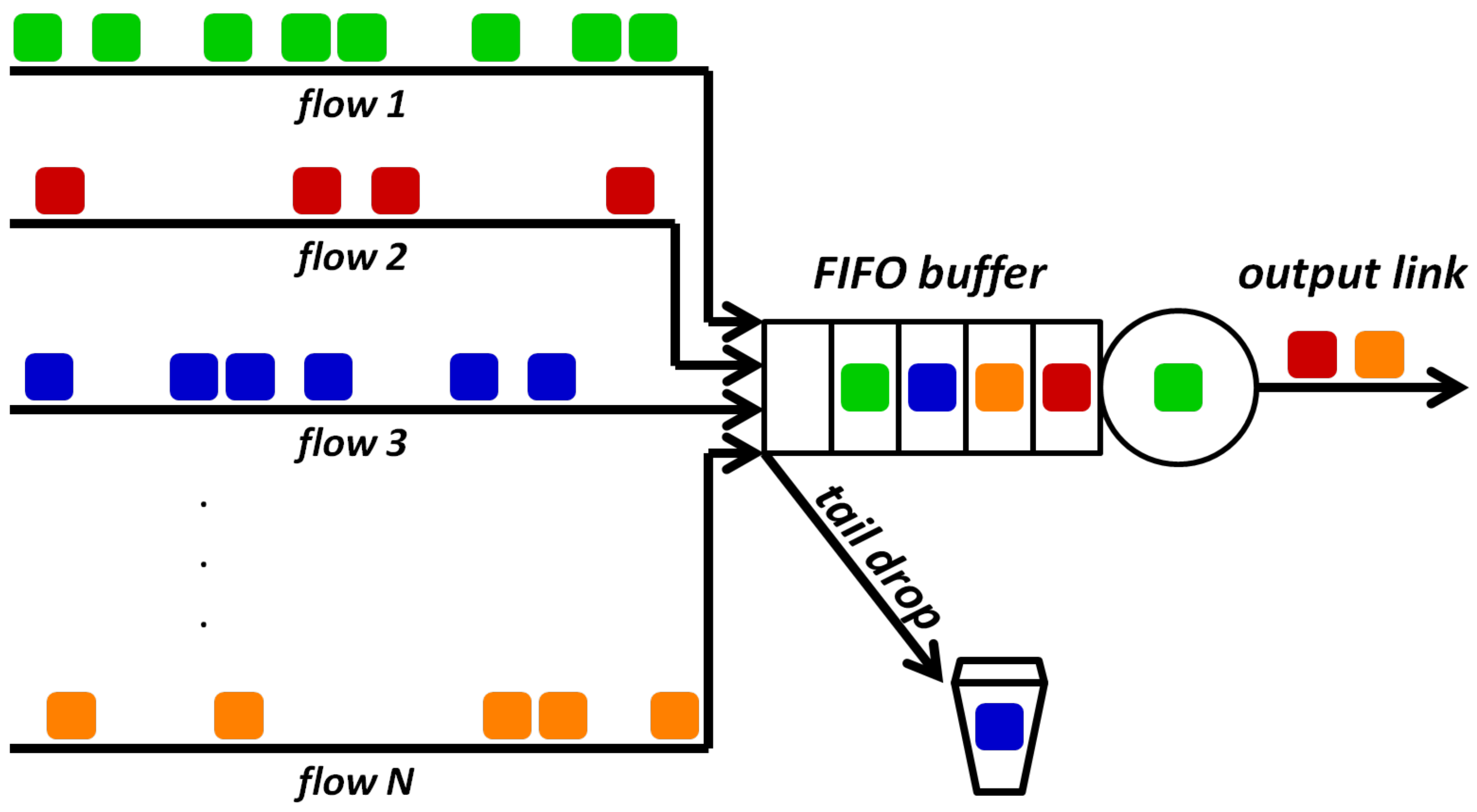
The full model considered here is schematically depicted in Figure 1.

Namely, consider N flows of packets arriving at a common FIFO buffer. Arriving packets are loaded into the buffer in order of arrival, regardless of the flow to which they belong.

Hence, a queue of packets is formed in the buffer. This queue is emptied from the head by an output link. The transmission (service) time of every packet is random and follows a distribution function $F\left(t\right)$, which may be arbitrary.

The buffer volume is K packets, including the first position, which is occupied by the packet in transmission, if the buffer is not empty.

When the buffer contains K packets, every newly arriving packet is discarded. This mechanism (tail drop) may potentially decrease the throughput of all flows.

Each flow may have a different, possibly complex interarrival time distribution. To model this, each flow is represented by a separate Markovian Arrival Process (MAP) (see, e.g., [13]).

Thus, there are N separate MAP processes in the full model: MAP₁, …, MAP_n. Specifically, flow number n is parameterized by matrices ${\mathbf{D}}_0^n$ and ${\mathbf{D}}_1^n$, each of size $M_n\times M_n$, where $M_n$ is the number of modulating states of MAP_n. Naturally, flows may have distinct statistical properties, so all matrices ${\mathbf{D}}_0^n$, ${\mathbf{D}}_1^n$, as well as their sizes $M_n\times M_n$, may differ from one another.

The following notations of parameters of flows, aggregate traffic and service process are employed:

• ${\lambda }_n$: arrival rate of the n-th flow [pkts/s];
• $\lambda ={\sum }_{n=1}^N{\lambda }_n$: arrival rate of the aggregate traffic [pkts/s];
• ${\overline{\lambda }}_n=\lambda -{\lambda }_n$: rate of the background traffic for the n-th flow [pkts/s];
• $d_n$: standard deviation of the interarrival time of the n-th flow;
• $C{V}_n=d_n{\lambda }_n$: coefficient of variation of the interarrival time of the n-th flow;
• S: mean packet service (transmission) time.

Naturally, for full system parametrization, it suffices to specify the matrices ${\mathbf{D}}_0^n$ and ${\mathbf{D}}_1^n$, $n=1,\dots ,N$, the distribution $F\left(t\right)$, and the buffer size K. All the other parameters mentioned above, i.e., ${\lambda }_n$, $d_n$, $C{V}_n$, and S, can be computed either from the parameter matrices or from the distribution F.

The performance characteristics of interest are the throughput of the n-th flow, $T_n$, and the loss ratio of the n-th flow, $L_n$. The throughput $T_n$ is defined as the number of packets belonging to the n-th flow departing the buffer per second, averaged over an extended time span. It is therefore expressed in units of [pkts/s]. The loss ratio $L_n$ is the fraction of packets from the n-th flow that are discarded upon arrival at a full buffer, measured over a long time interval. Thus, $L_n$ is unitless and satisfies $L_n\in [0,1]$.

Moreover, T denotes the aggregate throughput, i.e., the total number of packets leaving the buffer per second, averaged over an extended time span, while L denotes the aggregate loss ratio, i.e., the fraction of all packets discarded upon arrival at a full buffer over a long time interval.

Obviously, it holds:

$$T={\displaystyle \sum _{n=1}^N}{T}_n,$$

(1)

and

$$L\lambda ={\displaystyle \sum _{n=1}^N}{L}_n{\lambda }_n.$$

(2)

Finally, the Laplace–Stieltjes transform of F will be needed in what follows:

$$f\left(s\right)={\int }_0^{\infty }{e}^{-sx}\mathrm{d}F\left(x\right),$$

(3)

and the system load:

$$\rho =\lambda S.$$

(4)

The full model presented in this section can mimic real multi-flow traffic with arbitrary precision due to the powerful modeling capabilities of MAP processes. Specifically, it is established that a MAP can capture not only the moments but also the exact shape of an arbitrary interarrival time distribution, as well as temporal correlations.

In [30,31,32], complex examples of very precise fitting Markovian processes to interarrival time distributions can be found. Other methods for fitting MAPs to trace files are available, e.g., in [33,34].

In theory, the full model defined above can be solved analytically. To achieve that, a Markov chain that keeps track of the modulating states of all flows, as well as the buffer occupancy, has to be used. Hence, the state space of this Markov chain must have $M_1{M}_2\dots M_N(K+1)$ elements, while the transition matrix $M_1^2{M}_2^2\dots M_N^2{(K+1)}^2$ entries.

For instance, if $N=10$ flows are considered, $M_1=\dots =M_N=3$ and $K=10$, the transition matrix has over 400 billion entries. Operating on such a matrix is beyond the limit of contemporary computational capabilities, while traffic consisting of only 10 flows is still a very modest scenario, without mentioning a very small buffer.

In other words, the analytical solution of the full model would involve extremely large matrices, even in modest practical cases. Hence, obtaining numerical results would be infeasible in most practical scenarios.

Therefore, in the next section, a simplified model is presented. The matrices involved in the simplified model are only of size $M_n\times M_n$, while the model remains quite accurate, as will be highlighted in the examples.

4. Simplified Model

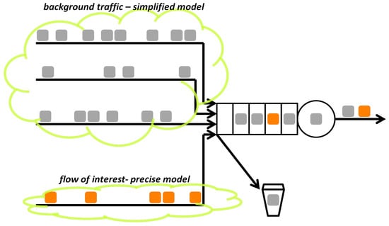
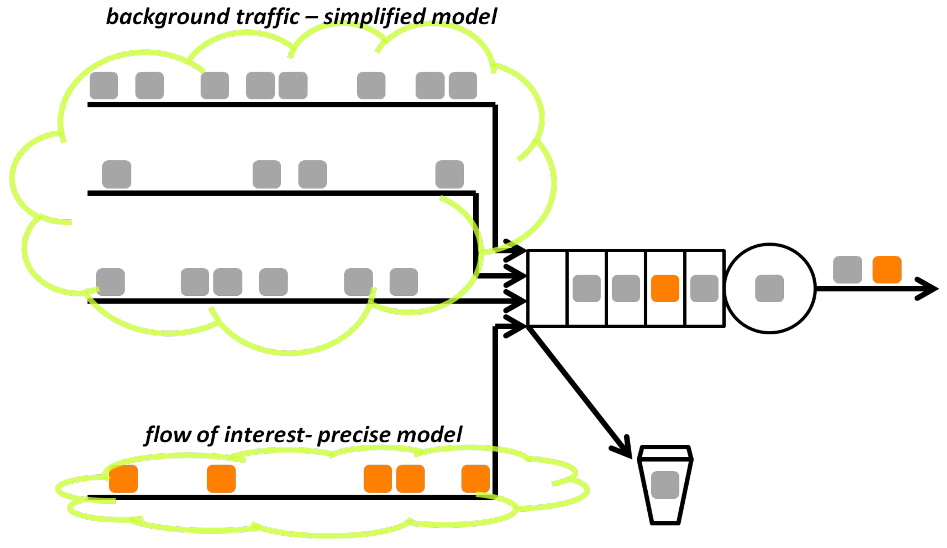
The idea of the simplified model is depicted in Figure 2.

Namely, assume that the throughput of a particular flow, say flow number n (orange packets in Figure 2), has to be computed. To obtain $T_n$, all flows except flow n are combined and constitute background traffic (grey packets in Figure 2). This background traffic is modeled as a Poisson process with intensity ${\overline{\lambda }}_n$. Flow n, however, is still modeled precisely by the MAP_n process using matrices ${\mathbf{D}}_0^n$ and ${\mathbf{D}}_1^n$.

Such a simplification of the full model has theoretical support based on the Palm–Khinchin limiting theorem (see, e.g., [35], page 146) concerning the convergence of the superposition of many point processes to a Poisson process. The applied simplification also indicates that, in typical situations, the model should be more accurate (i.e., closer to the full model when deriving $T_n$) as the total number of flows N increases. At the same time, it requires operations only on matrices of size $M_n\times M_n$, regardless of N. This is in sharp contrast to the matrices of size $N^{M_n}\times N^{M_n}$ required in the full model.

In the next section, exact formulae for throughput and loss ratio of the flow of interest (MAP_n) in the simplified model will be derived. Before that, some additional notation has to be introduced.

First, it is easy to see that the combined arrival process in the simplified model, consisting of the MAP_n process and a Poisson process of rate ${\overline{\lambda }}_n$, is stochastically equivalent to another Markovian process, denoted by MAP’. The parameter matrices of this MAP’ process are as follows:

$${\mathbf{D}}_0={\mathbf{D}}_0^n-{\overline{\lambda }}_n\mathbf{I},{\mathbf{D}}_1={\mathbf{D}}_1^n+{\overline{\lambda }}_n\mathbf{I},$$

(5)

where I denotes the identity matrix of dimension $M_n\times M_n$.

Let $J\left(t\right)$ denote the modulating state of the MAP’ process at time t, while $X\left(t\right)$ be the buffer occupancy at t in the simplified model, including the transmission position, if taken.

Several important characteristics of the simplified model are expressed in terms of the function $P_{i,j,m}\left(x\right)$, which is the probability that in a time interval of span x, m new packets arrive and modulating state at the end of the interval is j, given that at the beginning of the interval the modulating state was i.

In particular, the following two functionals based on $P_{i,j,k}\left(x\right)$ are very often in use:

$$a_{i,j,m}\left(s\right)={\int }_0^{\infty }{e}^{-st}{P}_{i,j,m}\left(x\right)\mathrm{d}F\left(x\right),$$

(6)

$$q_{i,j,m}\left(s\right)={\int }_0^{\infty }{e}^{-st}{P}_{i,j,m}\left(x\right)(1-F\left(x\right))\mathrm{d}x,$$

(7)

usually in the matrix form:

$${\mathbf{A}}_m\left(s\right)={\left[a_{i,j,m}\left(s\right)\right]}_{i,j=1,\dots ,M_n},$$

(8)

$${\mathbf{Q}}_m\left(s\right)={\left[q_{i,j,m}\left(s\right)\right]}_{i,j=1,\dots ,M_n}.$$

(9)

Matrices ${\mathbf{A}}_m$ and ${\mathbf{Q}}_m$ are commonly used in the analysis of queues with Markovian arrivals. Specifically, ${\mathbf{A}}_m\left(0\right)$ represents the probability that within a service interval, m new packets arrive and modulating state jumps from i to j in this interval, whereas ${\mathbf{Q}}_m\left(0\right)$ represents the probability that within a remaining service time in equilibrium, m new packets arrive and modulating state jumps from i to j.

The stationary distribution for the modulating process of (5) will be denoted by $\pi$. It may be calculated using the well-known relations:

$$\begin{array}{c}\hfill \left\{\begin{array}{c}\pi ({\mathbf{D}}_0+{\mathbf{D}}_1)=[0,\dots ,0],\hfill \\ \pi \mathbf{e}=1,\hfill \end{array}\right.\end{array}$$

(10)

where $\mathbf{e}={[1,\dots ,1]}^T$.

The probabilities $u_{i,j,m}$ of jump of the modulating state from i to j in MAP’, accompanied by arrival of a packet ($m=1$), or without arrival ($m=0$), can be computed as:

$$u_{i,i,0}=0,$$

(11)

$$u_{i,j,0}={\displaystyle \frac{1}{{\beta }_i}}{\left({\mathbf{D}}_0\right)}_{ij},i\ne j,$$

(12)

$$u_{i,j,1}={\displaystyle \frac{1}{{\beta }_i}}{\left({\mathbf{D}}_1\right)}_{ij}.$$

(13)

where

$${\beta }_i=-{\left({\mathbf{D}}_0\right)}_{ii},1\le i\le M_n.$$

(14)

Finally, the following square matrices are often of use:

$$0=\mathrm{zero} \mathrm{matrix},$$

(15)

$${\mathbf{U}}_m\left(s\right)={\left[{\displaystyle \frac{{\beta }_i{u}_{i,j,m}}{s+{\beta }_i}}\right]}_{i,j},m=0,1,$$

(16)

$${\mathbf{B}}_m\left(s\right)={\displaystyle \sum _{i=m}^{\infty }}{\mathbf{A}}_i\left(s\right)={\int }_0^{\infty }{e}^{-sx}{e}^{({\mathbf{D}}_0+{\mathbf{D}}_1)x}\mathrm{d}F\left(x\right)-{\displaystyle \sum _{i=0}^{m-1}}{\mathbf{A}}_i\left(s\right),$$

(17)

$${\mathbf{C}}_m\left(s\right)={\mathbf{A}}_{m+1}\left(s\right)-{\mathbf{B}}_{m+1}\left(s\right){\mathbf{B}}_0^{-1}\left(s\right),$$

(18)

$${\mathbf{R}}_0\left(s\right)=0,{\mathbf{R}}_1\left(s\right)={\mathbf{A}}_0^{-1}\left(s\right),$$

(19)

$${\mathbf{R}}_m\left(s\right)={\mathbf{A}}_0^{-1}\left(s\right)({\mathbf{R}}_{m-1}\left(s\right)-{\displaystyle \sum _{k=0}^{m-1}}{\mathbf{A}}_{k+1}\left(s\right){\mathbf{R}}_{m-k}\left(s\right)),m\ge 2.$$

Naturally, they are all of dimensions $M_n\times M_n$.

Matrices ${\mathbf{U}}_m$, ${\mathbf{B}}_m$ and ${\mathbf{C}}_m$ have no special meaning. They are just used to shorten the notation of equations and formulae. Sequence ${\mathbf{R}}_m$ plays a special role because equations characterizing the performance of Markovian queues often have solutions that can be presented in a similar, specific form involving ${\mathbf{R}}_m$ (see Lemma 3.2.1 of [36]).

It was already mentioned that a MAP process can accurately capture virtually any form of the interarrival-time distribution, its moments, and the temporal correlation. In the full model, a separate MAP process is assigned to each flow, potentially with different forms of all these characteristics.

At first glance, it may appear that the simplified model of this section loses this information for all flows except one. However, this apparent loss is somewhat misleading.

Note that when analyzing a real system with N flows, the simplified model is not used just once, but N times–each time preserving the statistical properties and structure of a different flow. In other words, the full model is effectively replaced not by a single simplified model, but by N such models. Taken together, these N models retain all the information for all flows.

5. Exact Solution of the Simplified Model

Assuming the model of the previous section, the following theorem will be proven.

Theorem 1. 

The throughput of MAP_n flow equals:

$$T_n={\displaystyle \frac{1-p_0}{S}}+p_K{\overline{\lambda }}_n-{\overline{\lambda }}_n,$$

(20)

while the loss ratio of MAP_n flow equals:

$$L_n={\displaystyle \frac{\lambda }{{\lambda }_n}}-{\displaystyle \frac{1-p_0}{S{\lambda }_n}}-p_k{\displaystyle \frac{\overline{{\lambda }_n}}{{\lambda }_n}},$$

(21)

where

$$p_0=\underset{s\to 0+}{lim}s\pi {\mathbf{G}}^{-1}\left(s\right){\mathbf{w}}_0\left(s\right),$$

(22)

$$p_K=\underset{s\to 0+}{lim}s\pi {\mathbf{G}}^{-1}\left(s\right){\mathbf{w}}_K\left(s\right),$$

(23)

$$\begin{array}{cc}\hfill \mathbf{G}\left(s\right)=& \left(\mathbf{I}-{\mathbf{U}}_0\left(s\right)\right)\left({\mathbf{R}}_{k+1}\left(s\right){\mathbf{A}}_0\left(s\right)+{\displaystyle \sum _{k=0}^K}{\mathbf{R}}_{K-k}\left(s\right){\mathbf{C}}_k\left(s\right)\right)\hfill \\ \hfill & -{\mathbf{U}}_1\left(s\right)\left({\mathbf{R}}_k\left(s\right){\mathbf{A}}_0\left(s\right)+{\displaystyle \sum _{k=0}^{K-1}}{\mathbf{R}}_{K-k-1}\left(s\right){\mathbf{C}}_k\left(s\right)\right),\hfill \end{array}$$

(24)

$${\mathbf{w}}_l\left(s\right)={\mathbf{U}}_1\left(s\right){\displaystyle \sum _{k=0}^{K-1}}{\mathbf{R}}_{K-k-1}\left(s\right){\mathbf{v}}_{k,l}\left(s\right)-\left(\mathbf{I}-{\mathbf{U}}_0\left(s\right)\right){\displaystyle \sum _{k=0}^K}{\mathbf{R}}_{K-k}\left(s\right){\mathbf{v}}_{k,l}\left(s\right)+{\delta }_{0,l}\mathbf{b}\left(s\right),$$

(25)

$${\mathbf{v}}_{m,l}\left(s\right)={\mathbf{B}}_{m+1}\left(s\right){\mathbf{B}}_0^{-1}\left(s\right){\mathbf{r}}_{K,l}\left(s\right)-{\mathbf{r}}_{K-m,l}\left(s\right),$$

(26)

$${\mathbf{r}}_{m,l}\left(s\right)=\left\{\begin{array}{ccc}(1-f\left(s\right))/s·\mathbf{e}-{\displaystyle {\sum }_{k=0}^{K-m-1}}{\mathbf{Q}}_k\left(s\right)·\mathbf{e},\hfill & \mathrm{if}\hfill & l=K,\hfill \\ {\mathbf{Q}}_{l-m}\left(s\right)·\mathbf{e},\hfill & \mathrm{if}\hfill & m\le l<K,\hfill \\ 0·\mathbf{e},\hfill & \mathrm{if}\hfill & l<m,\hfill \end{array}\right.$$

$$\mathbf{b}\left(s\right)={\left[{(s+{\beta }_1)}^{-1},\dots ,{(s+{\beta }_{M_n})}^{-1}\right]}^T,$$

(27)

while ${\delta }_{0,l}=1$ if $l=0$ and ${\delta }_{0,l}=0$ otherwise.

Sketch of the proof. Initially, it is assumed (temporarily) that the stationary full-buffer probability, $p_K$, and the empty-buffer probability, $p_0$, are known.

In the first step of the proof, the loss ratio of the flow of interest, $L_n$, is computed as a function of $p_0$. This can be achieved using a simple relation between all the rates and loss ratios involved (formula (28)), as well as the well-known general relation between L and $p_0$ (formula (30)). The resulting formula for $L_n$, (31), contains the unknown loss ratio of the background traffic, ${\overline{L}}_n$.

Hence, in the next step of the proof, ${\overline{L}}_n$ must be eliminated. This is done using the fact that the probability of finding the buffer full at arbitrary times is the same as the probability of finding the buffer full at Poisson times (PASTA theorem). As the background traffic is Poisson, its loss ratio must be the same as the probability of finding the buffer full at arbitrary times (formula (32)).

Using this fact and the relation between the throughput and the loss ratio, in the next step, the final formulae for the flow of interest, i.e., (20) and (21), are obtained.

This is, however, not the end of the proof, because (20) and (21) depend on $p_0$ and $p_K$. The rest of the proof is therefore devoted to computing these two values.

To achieve that, in the next step, a set of equations for $H_{m,i,l}\left(t\right)$ is built. $H_{m,i,l}\left(t\right)$ denotes the probability of having l packets in the buffer at time t, given that there were m packets in the buffer at the initial time and the modulating state was i. This set of Equations (35) and (36), is obtained by conditioning on the time of the first event in the arrival process and the end of the first transmission time, respectively.

Equations (35) and (36) have a Volterra integral form. The easiest way to treat them is to apply the Laplace transform, which is done in the next step. Then, a solution of the resulting simplified set (43), (44) is obtained using the sequence ${\mathbf{R}}_m\left(s\right)$ and Lemma 3.2.1 of [36].

In the final step of the proof, the limit as $t\to \infty$ of $H_{m,i,0}\left(t\right)$ and $H_{m,i,K}\left(t\right)$ is computed, to obtain $p_0$ and $p_K$, respectively. From the final value theorem, it is known that this is equivalent to computing the limit as $s\to 0+$ of $s{h}_{m,i,0}\left(s\right)$ and $s{h}_{m,i,K}\left(s\right)$, respectively, where $h_{m,i,l}\left(s\right)$ is the Laplace transform of $H_{m,i,l}\left(t\right)$.

Proof of Theorem 1. 

Using an obvious formula:

$$L\lambda ={\overline{L}}_n{\overline{\lambda }}_n+L_n{\lambda }_n,$$

(28)

yields:

$$L_n={\displaystyle \frac{L\lambda -{\overline{L}}_n{\overline{\lambda }}_n}{{\lambda }_n}}.$$

(29)

Exploiting the relation between L and $p_0$:

$$L=1-{\displaystyle \frac{1-p_0}{\lambda S}},$$

(30)

together with formula (29), yields:

$$L_n={\displaystyle \frac{\lambda }{{\lambda }_n}}-{\displaystyle \frac{1-p_0}{S{\lambda }_n}}-{\overline{L}}_n{\displaystyle \frac{\overline{{\lambda }_n}}{{\lambda }_n}}.$$

(31)

Using PASTA property (see, e.g., [8], page 175), it can be concluded that for background traffic, its loss ratio equals the stationary full-buffer probability:

$${\overline{L}}_n=p_K.$$

(32)

The latter, together with (32), completes the proof of (21).

Having (21) and (20) can be obtained immediately by exploiting the relation:

$$T_n=(1-L_n){\lambda }_n.$$

(33)

Now what is left is to derive the missing probabilities $p_0$ and $p_K$, i.e., to prove formulae (22) and (23). Define:

$$H_{m,i,l}\left(t\right)=\mathbb{P}\{X\left(t\right)=l|X\left(0\right)=m,J\left(0\right)=i\}.$$

(34)

Assuming $X\left(0\right)=0$ and conditioning on y, i.e., the time of first event in the MAP’ (arrival, change of state, or both), it holds:

$$H_{0,i,l}\left(t\right)={\displaystyle \sum _{j=1}^{M_n}}{\displaystyle \sum _{k=0}^1}{\int }_0^t{H}_{k,j,l}(t-y)u_{i,j,k}{\beta }_i{e}^{-{\beta }_{i}y}\mathrm{d}y+{\delta }_{0,l}{e}^{-{\beta }_{i}t}.$$

(35)

Indeed, in MAP’ the time of the first event, denoted by y, has density ${\beta }_i{e}^{-{\beta }_{i}y}$. Assume first that $y<t$. At time y, the modulating state changes to j, either together with a packet arrival, with probability $u_{i,j,1}$, or without a packet arrival, with probability $u_{i,j,0}$. Therefore, at time y, either $\mathbb{P}\{X\left(t\right)=l\}=H_{1,j,l}(t-y)$ or $\mathbb{P}\{X\left(t\right)=l\}=H_{0,j,l}(t-y)$, depending on which case occurs.

If $y\ge t$, which happens with probability $e^{-{\beta }_{i}t}$, then $\mathbb{P}\{X\left(t\right)=l\}={\delta }_{0,l}$.

Assuming $X\left(0\right)>0$ and conditioning on x, i.e., the end of first transmission time, it holds:

$$\begin{array}{cc}\hfill H_{m,i,l}\left(t\right)=& {\displaystyle \sum _{j=1}^{M_n}}{\displaystyle \sum _{k=0}^{K-m-1}}{\int }_0^t{H}_{m+k-1,j,l}(t-x)P_{i,j,k}\left(x\right)\mathrm{d}F\left(x\right)\hfill \\ \hfill & +{\displaystyle \sum _{j=1}^{M_n}}{\displaystyle \sum _{k=K-m}^{\infty }}{\int }_0^t{H}_{K-1,j,l}(t-x)P_{i,j,k}\left(x\right)dF\left(x\right)+r_{m,i,l}\left(t\right),m=1,\dots ,K,\hfill \end{array}$$

(36)

where

$$r_{m,i,l}\left(t\right)=(1-F\left(t\right))·\left\{\begin{array}{ccc}{\displaystyle {\sum }_{j=1}^{M_n}}{\displaystyle {\sum }_{k=K-m}^{\infty }}{P}_{i,j,k}\left(t\right),\hfill & if\hfill & l=K,\hfill \\ {\displaystyle {\sum }_{j=1}^{M_n}}{P}_{i,j,l-m}\left(t\right),\hfill & if\hfill & m\le l<K,\hfill \\ 0,\hfill & if\hfill & l<m.\hfill \end{array}\right.$$

(37)

Namely, the first component of (36) reflects the situation in which the first transmission is completed by time t (i.e., $x<t$) and $k<K-m$ new packets arrive by time x, so the buffer is not full before x. In this case, immediately after the first packet departs at time x, it holds $\mathbb{P}\{X\left(t\right)=l\}=H_{m+k-1,j,l}(t-x)$. The second component of (36) represents the situation where again $x<t$, but $k\ge K-m$ new packets arrive by time x, making the buffer full before x. Hence, at time x, immediately after the first departure, it holds $\mathbb{P}\{X\left(t\right)=l\}=H_{K-1,j,l}(t-x)$. The third component, $r_{m,i,l}\left(t\right)$, represents the situation where $x\ge t$, which occurs with probability $1-F\left(t\right)$. In this case, the formula for $\mathbb{P}\left\{X\right(t)=l\}$ depends on l. Specifically, $l=K$ at time t can happen only if $k\ge K-m$ new packets arrive by t, which has probability ${\sum }_{k=K-m}^{\infty }{P}_{i,j,k}\left(t\right)$, as expressed in the first component of (37). Then, for $m\le l<K$, the probability is $P_{i,j,l-m}\left(t\right)$, while $l<m$ is impossible.

Denoting:

$$h_{m,i,l}\left(s\right)={\int }_0^{\infty }{e}^{-sx}{H}_{m,i,l}\left(x\right)dx,$$

(38)

Equations (35) and (36) yield:

$$h_{0,i,l}\left(s\right)={\displaystyle \sum _{j=1}^{M_n}}{\displaystyle \sum _{k=0}^1}{u}_{i,j,k}{h}_{k,j,l}\left(s\right){\displaystyle \frac{{\beta }_i}{s+{\beta }_i}}+{\delta }_{0,l}{\displaystyle \frac{1}{s+{\beta }_i}},$$

(39)

and

$$\begin{array}{cc}\hfill h_{m,i,l}\left(s\right)=& {\displaystyle \sum _{j=1}^{M_n}}{\displaystyle \sum _{k=0}^{K-m-1}}{a}_{k,i,j}\left(s\right)h_{m+k-1,j,l}\left(s\right)\hfill \end{array}$$

(40)

$$\begin{array}{cc}\hfill & +{\displaystyle \sum _{j=1}^{M_n}}{\displaystyle \sum _{k=K-m}^{\infty }}{a}_{k,i,j}\left(s\right)h_{K-1,j,l}\left(s\right)+{\int }_0^{\infty }{e}^{-sx}{r}_{m,i,l}\left(x\right)\mathrm{d}x,m=1,\dots ,K,\hfill \end{array}$$

(41)

respectively. Using vectors:

$${\mathbf{h}}_{m,l}\left(s\right)={[h_{m,1,l}\left(s\right),\dots ,h_{m,M_n,l}\left(s\right)]}^T,$$

(42)

(39) and (40) yield:

$${\mathbf{h}}_{0,l}\left(s\right)={\displaystyle \sum _{k=0}^1}{\mathbf{U}}_k\left(s\right){\mathbf{h}}_{k,l}\left(s\right)+{\delta }_{0,l}\mathbf{b}\left(s\right),$$

(43)

$${\mathbf{h}}_{m,l}\left(s\right)={\displaystyle \sum _{k=0}^{K-m-1}}{\mathbf{A}}_k\left(s\right){\mathbf{h}}_{m+k-1,l}\left(s\right)+{\displaystyle \sum _{k=K-m}^{\infty }}{\mathbf{A}}_k\left(s\right){\mathbf{h}}_{K-1,l}\left(s\right)+{\mathbf{r}}_{m,l}\left(s\right),m=1,\dots ,K,$$

(44)

respectively. Exploiting the replacement of variables as follows:

$${\widehat{\mathbf{h}}}_{m,l}\left(s\right)={\mathbf{h}}_{K-m,l}\left(s\right),$$

(45)

Equations (43) and (44) transform to:

$${\widehat{\mathbf{h}}}_{K,l}\left(s\right)={\displaystyle \sum _{k=K-1}^K}{\mathbf{U}}_{K-k}\left(s\right){\widehat{\mathbf{h}}}_{k,l}\left(s\right)+{\delta }_{0,l}\mathbf{b}\left(s\right),$$

(46)

$${\displaystyle \sum _{k=-1}^m}{\mathbf{A}}_{k+1}\left(s\right){\widehat{\mathbf{h}}}_{m-k,l}\left(s\right)-{\widehat{\mathbf{h}}}_{m,l}\left(s\right)={\mathbf{x}}_{m,l}\left(s\right),m=0,\dots ,K-1,$$

(47)

respectively, with:

$${\mathbf{x}}_{m,l}\left(s\right)={\mathbf{A}}_{m+1}\left(s\right){\widehat{\mathbf{h}}}_{0,l}\left(s\right)-{\displaystyle \sum _{k=m+1}^{\infty }}{\mathbf{A}}_k\left(s\right){\widehat{\mathbf{h}}}_{1,l}\left(s\right)-{\mathbf{r}}_{K-m,l}\left(s\right).$$

(48)

From Lemma 3.2.1 of [36], it can be deduced that Equation (47) has the solution:

$${\widehat{\mathbf{h}}}_{m,l}\left(s\right)={\mathbf{R}}_{m+1}\left(s\right){\mathbf{c}}_l\left(s\right)+{\displaystyle \sum _{k=0}^m}{\mathbf{R}}_{m-k}\left(s\right){\mathbf{x}}_{k,l}\left(s\right),m=0,\dots ,K-1,$$

(49)

where ${\mathbf{c}}_l\left(s\right)$ is an unknown vector independent of m. Using (49) with $m=0$ yields:

$${\mathbf{c}}_l\left(s\right)={\mathbf{A}}_0\left(s\right){\widehat{\mathbf{h}}}_{0,l}\left(s\right),$$

(50)

whereas using (47) with $m=0$ yields:

$${\widehat{\mathbf{h}}}_{1,l}\left(s\right)={\mathbf{B}}_0^{-1}\left(s\right)({\widehat{\mathbf{h}}}_{0,l}\left(s\right)-{\mathbf{r}}_{K,l}\left(s\right)).$$

(51)

Then, exploiting (46) we arrive at:

$${\widehat{\mathbf{h}}}_{0,l}\left(s\right)={\mathbf{h}}_{K,l}\left(s\right)={\mathbf{G}}^{-1}\left(s\right){\mathbf{w}}_l\left(s\right),$$

(52)

where $\mathbf{G}\left(s\right)$ and ${\mathbf{w}}_l\left(s\right)$ are given in (24) and (25), respectively.

Having ${\mathbf{h}}_{K,l}\left(s\right)$, one can quickly determine the empty and full buffer probabilities by applying the final value theorem. Namely, it holds:

$$p_0=\underset{s\to 0+}{lim}s\pi {\mathbf{h}}_{K,0}\left(s\right),$$

(53)

$$p_K=\underset{s\to 0+}{lim}s\pi {\mathbf{h}}_{K,K}\left(s\right).$$

(54)

(Note that the initial state vector, $\pi$, does not influence the stationary outcome, so any other can be used instead, e.g., $[1,0,\dots ,0]$.

Therefore, (53) and (54), combined with (52), complete the proof of Theorem 1. □

It is essential to highlight that all matrices used in Theorem 1 are of small size, i.e., $M_n\times M_n$, and can be computed numerically. In particular, the matrices ${\mathbf{A}}_m\left(s\right)$ and ${\mathbf{Q}}_m\left(s\right)$ can be calculated via the uniformization method (see [13], page 66), ${\mathbf{U}}_m\left(s\right)$ are trivial, while the matrices ${\mathbf{B}}_m\left(s\right)$, ${\mathbf{C}}_m\left(s\right)$, and ${\mathbf{R}}_m\left(s\right)$ can be computed using ${\mathbf{A}}_m\left(s\right)$. The limit $s\to 0^{+}$ in (22) and (23) can be calculated numerically by using small values of s and observing convergence. In the examples shown in the next section, $s={10}^{-7}$ is used.

It is easy to check that the number of flops needed in a single application of the formulae of Theorem 1 grows as $\mathcal{O}\left(M_n^3{K}^2\right)$, assuming the cost of inversion and multiplication of $M_n\times M_n$ matrices is $\mathcal{O}\left(M_n^3\right)$. The primary expense is linked to the calculation of the matrices $R_m\left(s\right)$ from (19).

When solving the multi-flow system with respect to every flow, we need to apply Theorem 1 N times. Hence, the cost of obtaining the complete solution grows as $\mathcal{O}\left(N{M}^3{K}^2\right)$, where $M=max\{M_1,\dots ,M_N\}$.

The complexity of solving the simplified model, $\mathcal{O}\left(N{M}^3{K}^2\right)$, is in striking contrast with that of solving the full model, which would be $\mathcal{O}(M_1^3{M}_2^3\dots M_N^3{K}^3)$, or simply $\mathcal{O}\left(M^{3N}{K}^3\right)$ when $M=M_1=\dots =M_N$.

Finally, Theorem 1 may have two main areas of application. First, it may be used to compute the throughput values of flows in a concrete, practical networking scenario. For this, a precise estimation of MAP matrices is needed, which can be performed using one of the methods of [30,31,32,33,34], assuming precise knowledge of arrival statistics is available.

The second area of application of Theorem 1 is to provide general insight into the impact of particular system parameters on the throughput values of individual flows. For instance, we can answer the following questions using Theorem 1: How will the throughputs of the flows change when the buffer size changes from 50 to 100? How will the throughputs of the flows change if flow rate proportions change from 1:2:3 to 1:9:50? How will the throughputs of the flows change if the number of flows increases from 90 to 900? How will the throughputs of the flows change if the load drops from 100% to 70%? The answers to many such questions can be found in the next section.

6. Examples

In the examples, flows with three different coefficients of variation of the interarrival time: $CV=1$, $CV=2$, and $CV=5$ will be used. The latter value represents very high variability of the interarrival time; $CV=2$ is still quite high, and $CV=1$ is moderate. Moreover, the flows will have three different arrival rates: 100, 200, and 300 pkts/s.

Combining the three coefficients of variation with the three arrival rates gives $N=9$ flows in total, each with a distinct statistical characterization. The specific parameterizations of the nine flows, chosen to satisfy the assumptions of the previous paragraph, are as follows:

Flow 1: ${\lambda }_1=100$ pkts/s, $C{V}_1=1$, MAP₁ matrices:

$${\mathbf{D}}_0^1=\left[\begin{array}{cc}\hfill -100& \hfill 0\\ \hfill 0& \hfill -100\end{array}\right],{\mathbf{D}}_1^1=\left[\begin{array}{cc}\hfill 50& \hfill 50\\ \hfill 50& \hfill 50\end{array}\right].$$

(55)

Flow 2: ${\lambda }_2=200$ pkts/s, $C{V}_2=1$, MAP₂ matrices:

$${\mathbf{D}}_0^2=\left[\begin{array}{cc}\hfill -200& \hfill 0\\ \hfill 0& \hfill -200\end{array}\right],{\mathbf{D}}_1^2=\left[\begin{array}{cc}\hfill 100& \hfill 100\\ \hfill 100& \hfill 100\end{array}\right].$$

(56)

Flow 3: ${\lambda }_3=300$ pkts/s, $C{V}_3=1$, MAP₃ matrices:

$${\mathbf{D}}_0^3=\left[\begin{array}{cc}\hfill -300& \hfill 0\\ \hfill 0& \hfill -300\end{array}\right],{\mathbf{D}}_1^3=\left[\begin{array}{cc}\hfill 150& \hfill 150\\ \hfill 150& \hfill 150\end{array}\right].$$

(57)

Flow 4: ${\lambda }_4=100$ pkts/s, $C{V}_4=2$, MAP₄ matrices:

$${\mathbf{D}}_0^4=\left[\begin{array}{cc}\hfill -39.3393& \hfill 0\\ \hfill 0& \hfill -3672.2177\end{array}\right],{\mathbf{D}}_1^4=\left[\begin{array}{cc}\hfill 15.2174& \hfill 24.1219\\ \hfill 1420.5009& \hfill 2251.7168\end{array}\right].$$

(58)

Flow 5: ${\lambda }_5=200$ pkts/s, $C{V}_5=2$, MAP₅ matrices:

$${\mathbf{D}}_0^5=\left[\begin{array}{cc}\hfill -78.6785& \hfill 0\\ \hfill 0& \hfill -7344.4355\end{array}\right],{\mathbf{D}}_1^5=\left[\begin{array}{cc}\hfill 30.4347& \hfill 48.2438\\ \hfill 2841.0018& \hfill 4503.4337\end{array}\right].$$

(59)

Flow 6: ${\lambda }_6=300$ pkts/s, $C{V}_6=2$, MAP₆ matrices:

$${\mathbf{D}}_0^6=\left[\begin{array}{cc}\hfill -118.0178& \hfill 0\\ \hfill 0& \hfill -11016.6531\end{array}\right],{\mathbf{D}}_1^6=\left[\begin{array}{cc}\hfill 45.6521& \hfill 72.3657\\ \hfill 4261.5026& \hfill 6755.1505\end{array}\right].$$

(60)

Flow 7: ${\lambda }_7=100$ pkts/s, $C{V}_7=5$, MAP₇ matrices:

$${\mathbf{D}}_0^7=\left[\begin{array}{cc}\hfill -7.6208& \hfill 0\\ \hfill 0& \hfill -9932.5811\end{array}\right],{\mathbf{D}}_1^7=\left[\begin{array}{cc}\hfill 0.5754& \hfill 7.0454\\ \hfill 749.8932& \hfill 9182.6879\end{array}\right].$$

(61)

Flow 8: ${\lambda }_8=200$ pkts/s, $C{V}_8=5$, MAP₈ matrices:

$${\mathbf{D}}_0^8=\left[\begin{array}{cc}\hfill -15.2415& \hfill 0\\ \hfill 0& \hfill -19865.1622\end{array}\right],{\mathbf{D}}_1^8=\left[\begin{array}{cc}\hfill 1.1507& \hfill 14.0908\\ \hfill 1499.7864& \hfill 18365.3758\end{array}\right].$$

(62)

Flow 9: ${\lambda }_9=300$ pkts/s, $C{V}_9=5$, MAP₉ matrices:

$${\mathbf{D}}_0^9=\left[\begin{array}{cc}\hfill -22.8623& \hfill 0\\ \hfill 0& \hfill -29797.7433\end{array}\right],{\mathbf{D}}_1^9=\left[\begin{array}{cc}\hfill 1.7261& \hfill 21.1362\\ \hfill 2249.6796& \hfill 27548.0637\end{array}\right].$$

(63)

It is straightforward to determine the aggregate arrival rate: $\lambda =1800$ pkts/s.

A highly variable distribution for the service time will be used; specifically, a gamma distribution with parameters $\alpha =0.25$ and $\theta =0.0022222222$. Hence, the service rate is 1800 pkts/s and $\rho =1$ (the system is fully loaded), while the packet service time has a coefficient of variation of 2.

In every scenario and for each considered flow, the results obtained from a simulation of the full model of Section 3 and the results derived via the simplified model and Theorem 1 will be compared. All simulations were implemented and run in OMNeT++, version 6.3, [37]. In scenarios with 3 and 9 flows, $2\times {10}^8$ packets were used in simulations, while in scenarios with 90 and 900 flows, it was $2\times {10}^9$ and $2\times {10}^{10}$ packets, respectively. These large numbers of simulated packets enabled obtaining the per-flow throughput with a precision of 0.1 pkts/s, which was confirmed in 5 runs of each simulation. This precision is therefore used in all the tables below.

Firstly, the per-flow throughput for a very small FIFO buffer, $K=20$, will be examined. The results are presented in

Table 2. Simulated and derived throughput for all flows. $K=20$, $\rho =1$, gamma service with $CV=2$.

Flow Number	1	2	3	4	5	6	7	8	9
simulated throughput [pks/s]	91.3	182.6	273.9	87.8	174.7	261.5	61.6	117.1	172.5
derived throughput [pks/s]	89.8	179.6	269.4	85.2	169.3	253.4	56.9	110.8	166.6
relative error	1.6%	1.6%	1.6%	3.0%	3.1%	3.1%	7.5%	5.4%	3.4%

.

As shown in Table 2, the maximum relative error of throughput prediction provided by Theorem 1 is $7.5\%$, and about 2–$3\%$ for the majority of flows. The error is higher for the highly variable flows 7–9. Among these, the worst result is observed for flow 7, where very high variability is combined with a relatively low arrival rate.

This maximum error of $7.5\%$ can be considered satisfactory because the scenario in Table 2 is particularly challenging. Specifically, the buffer is very small, there are very few flows (so the limiting theorem is barely applicable), the flows are highly diverse in terms of coefficient of variation and rate, and the service time is highly variable.

Let us now examine the effect of increasing the buffer size on the per-flow throughput.

Table 3. Simulated and derived throughput for all flows. $K=50$, $\rho =1$, gamma service with $CV=2$.

Flow Number	1	2	3	4	5	6	7	8	9
simulated throughput [pks/s]	95.4	191.0	286.3	93.7	186.8	280.2	79.4	156.1	233.0
derived throughput [pks/s]	95.4	190.8	286.2	93.3	186.1	278.9	77.8	154.2	231.3
relative error	0.0%	0.1%	0.0%	0.4%	0.4%	0.5%	2.1%	1.2%	0.7%

and

Table 4. Simulated and derived throughput for all flows. $K=100$, $\rho =1$, gamma service with $CV=2$.

Flow Number	1	2	3	4	5	6	7	8	9
simulated throughput [pks/s]	97.4	194.9	292.4	96.5	192.8	288.8	88.5	175.1	262.5
derived throughput [pks/s]	97.6	195.2	292.8	96.5	192.7	289.0	88.1	175.1	262.3
relative error	0.2%	0.2%	0.2%	0.0%	0.0%	0.1%	0.5%	0.0%	0.1%

present the results for buffer sizes of 50 and 100 packets, respectively.

For a buffer of 50 packets–which is still relatively small–the maximum error is only 2.1%, and less than 1% for the majority of flows. For $K=100$ packets, the maximum error drops to 0.5%, and the simplified model becomes highly accurate.

Furthermore, it is evident that increasing the buffer size leads to an increase in per-flow throughput in all considered cases (see Table 2, Table 3 and Table 4 for a comparison across individual flows).

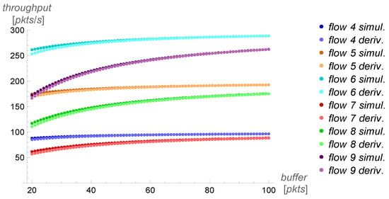
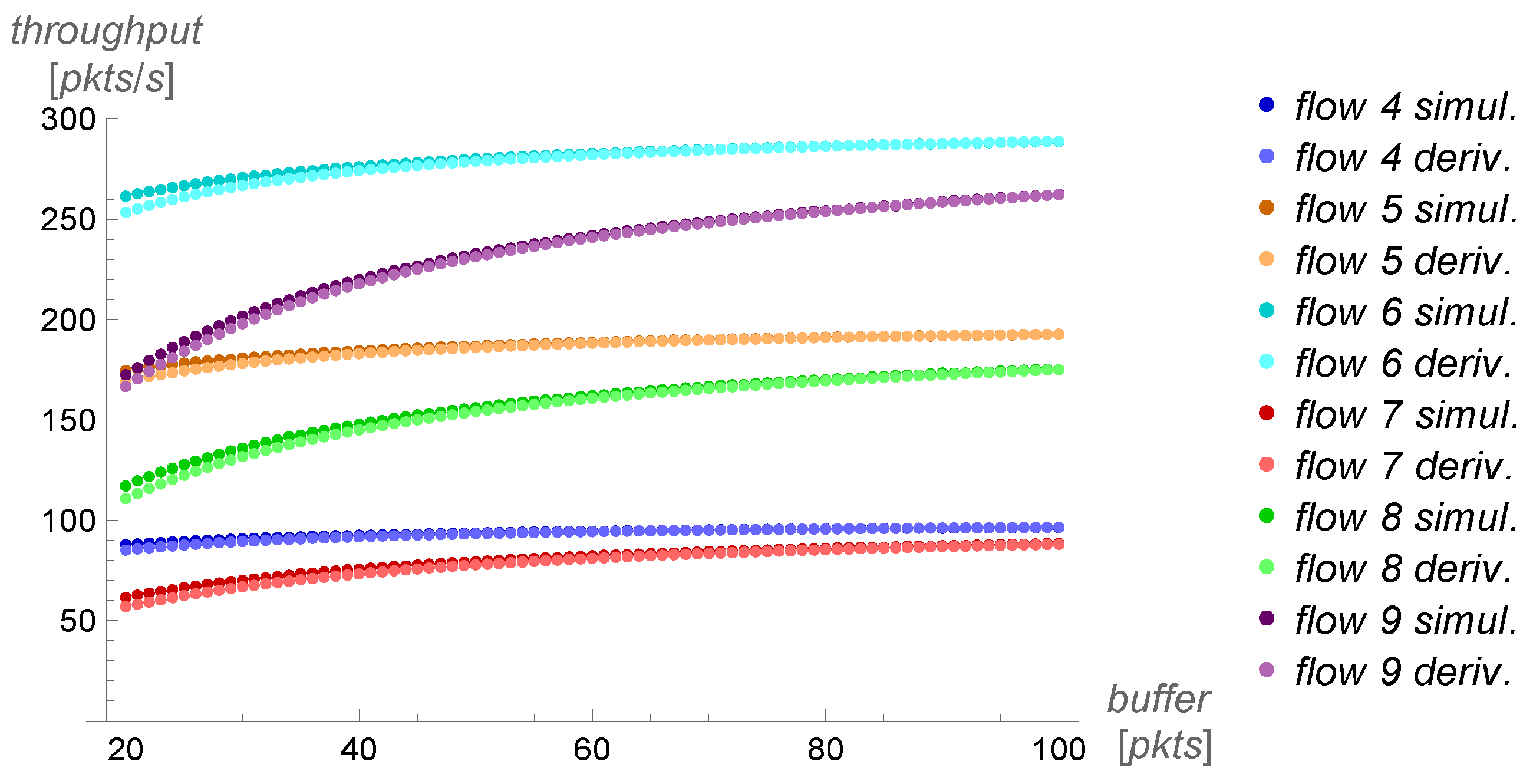
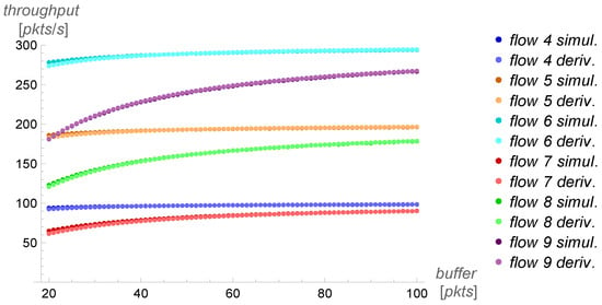
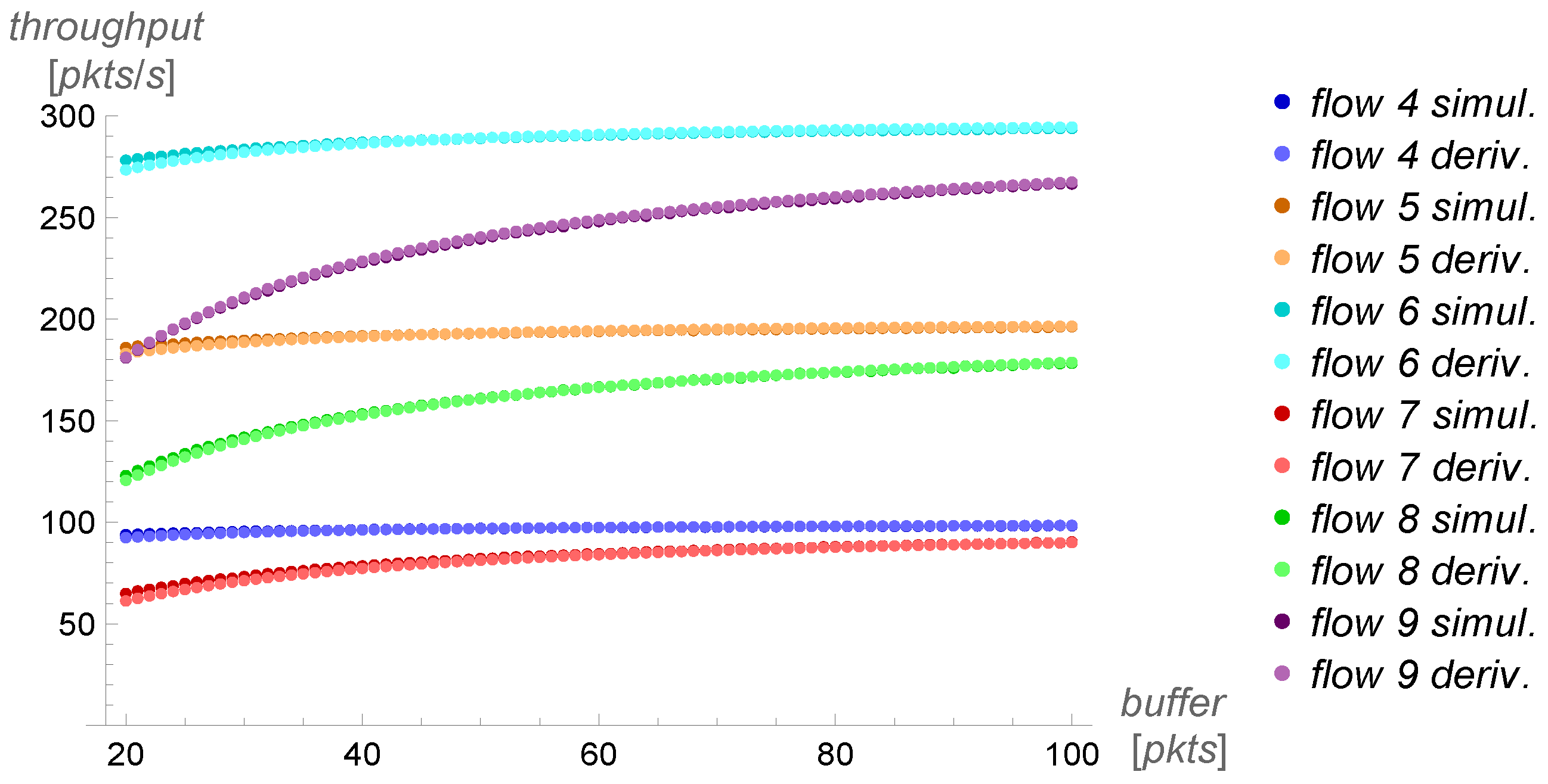
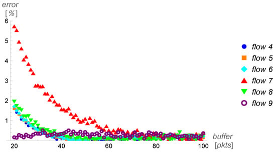
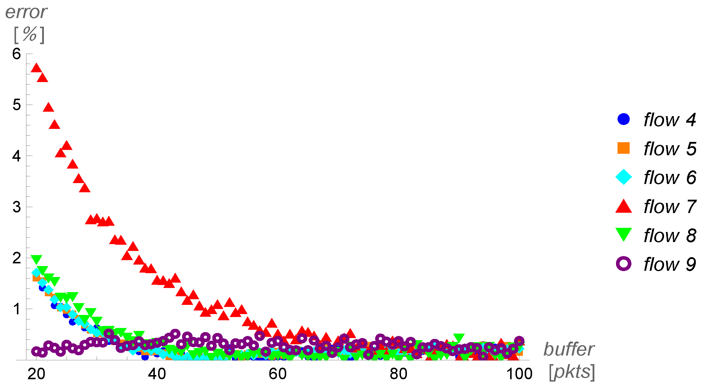
In Figure 3, the full dependence of the simulated and derived per-flow throughput for all buffer sizes in the range 20–100 packets is shown. To keep Figure 3 readable, only six selected flows are depicted, namely flows 4–9, which produced the largest errors in Table 2.

As seen in Figure 3, the curves derived using Theorem 1 largely overlap the simulated curves. Differences are noticeable only for relatively small buffers.

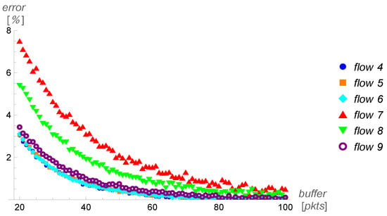
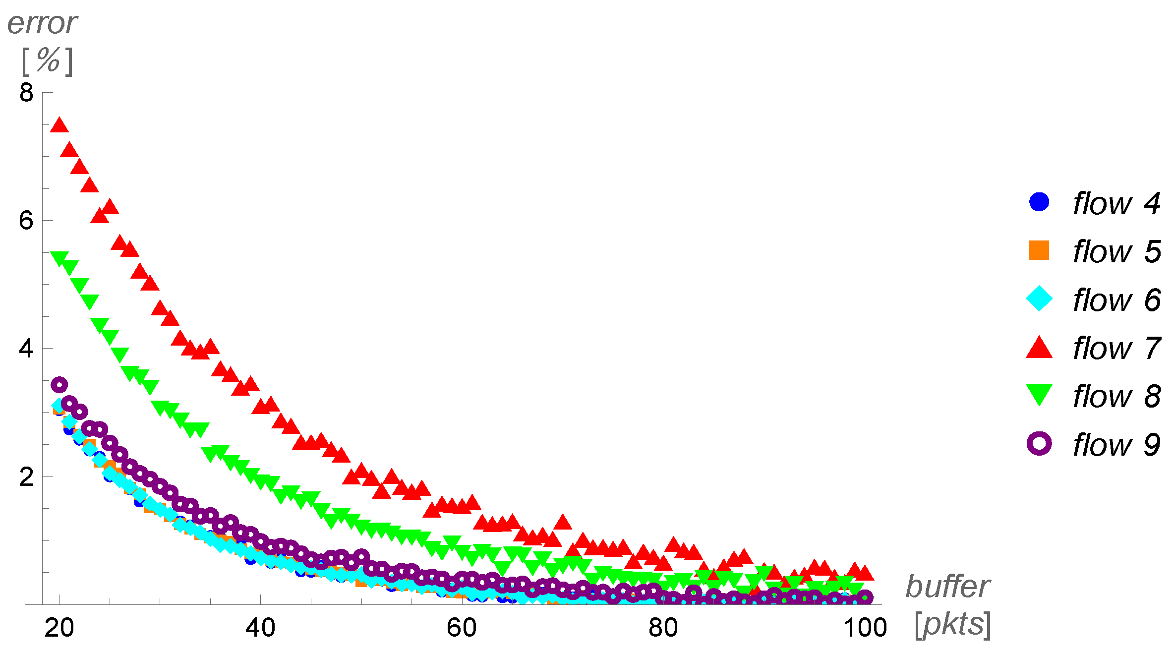
These differences, expressed as relative errors, are shown separately in Figure 4. As observed, the error generally decreases with increasing buffer size, and this trend holds for every flow in Figure 4.

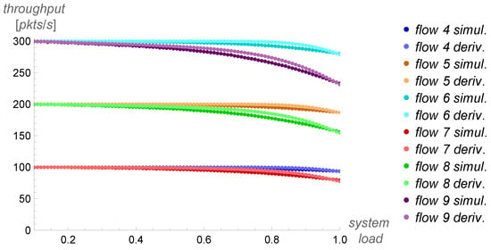
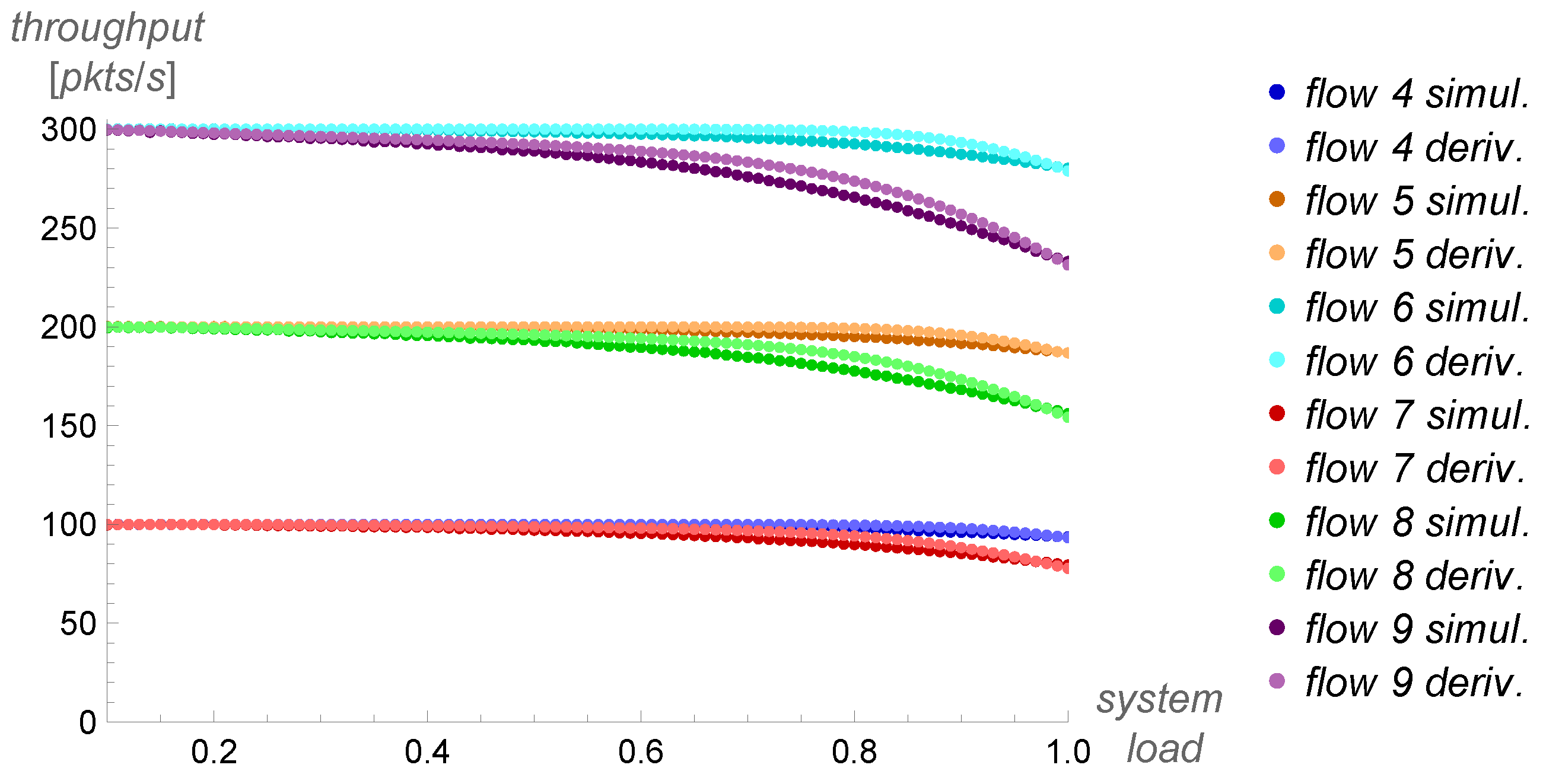
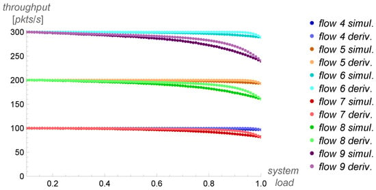
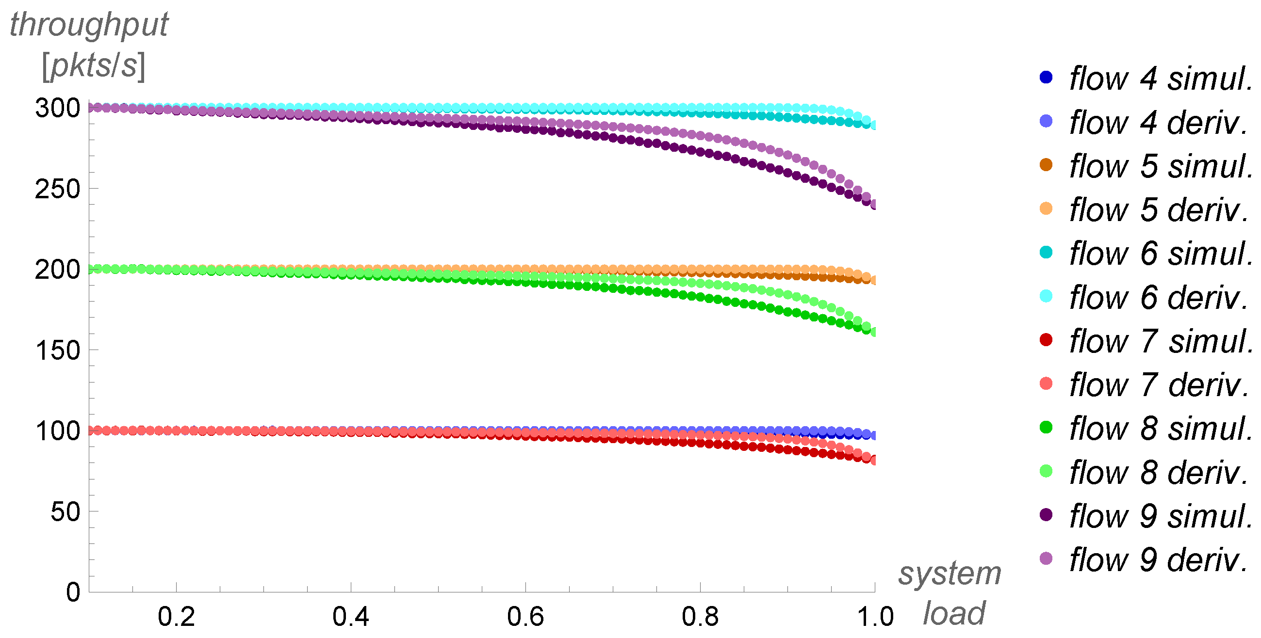
So far, only scenarios with full load ($\rho =1$) have been considered. Now we may examine what happens when the load is lower than that. To vary the load, the parameter $\theta$ of the service time may be scaled. This operation modifies the service rate while preserving the coefficient of variation, which remains equal to 2.

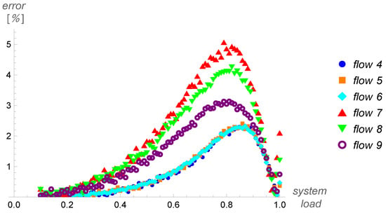
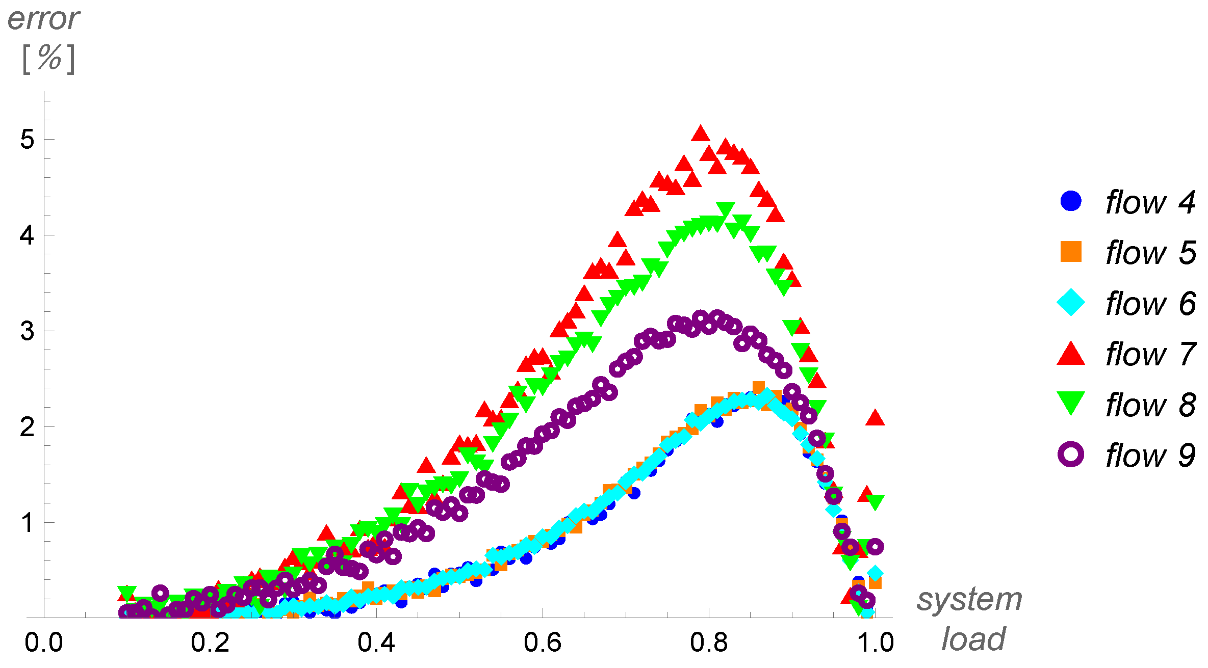
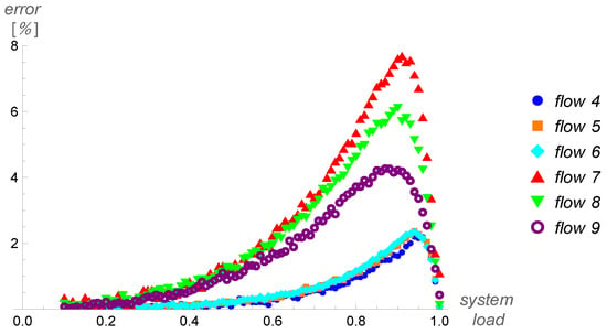
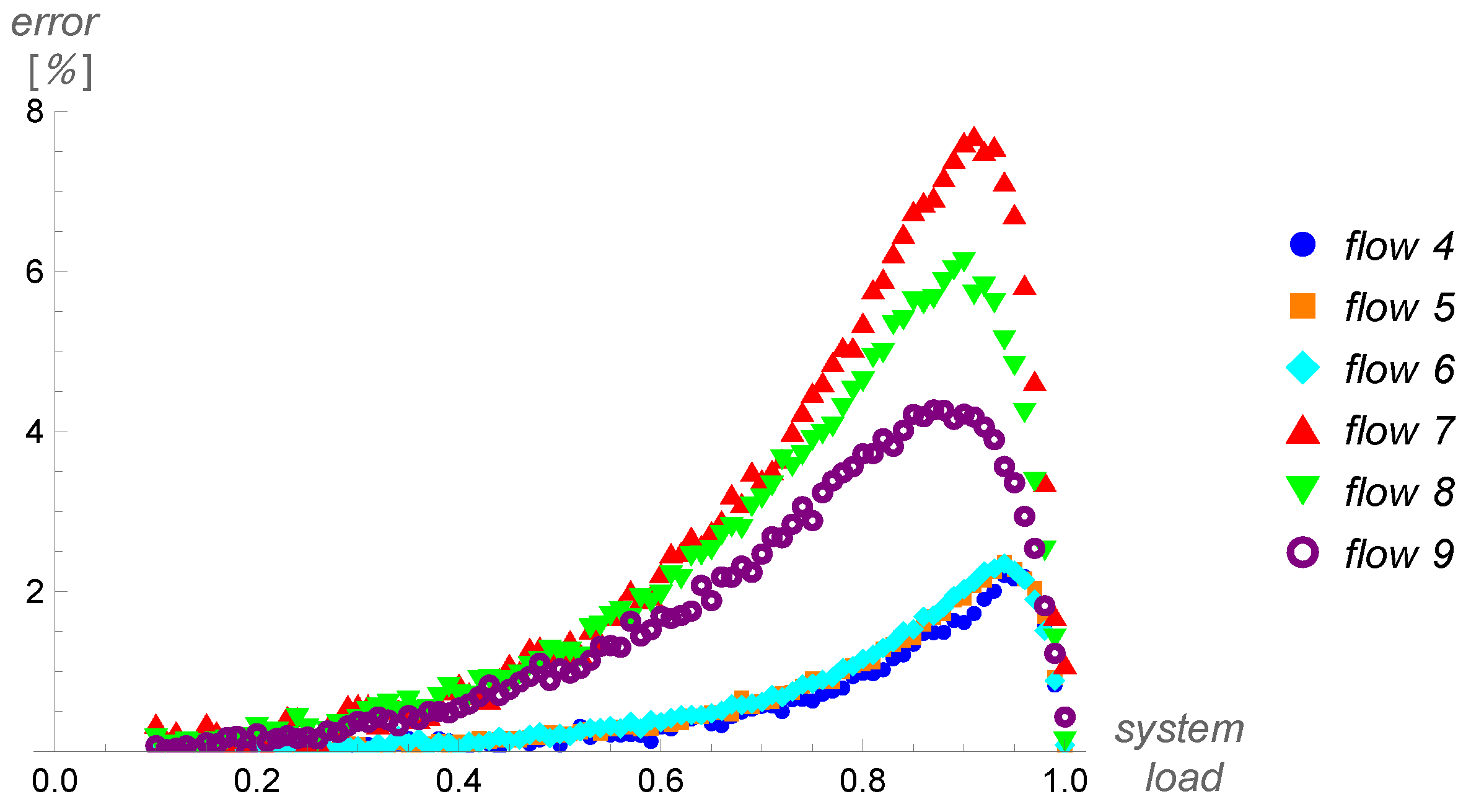
In Figure 5, the simulated and derived per-flow throughput is shown as a function of the system load, varying from 0.1 to 1. Figure 6 presents the corresponding relative errors.

As seen in Figure 5 and Figure 6, the error does not change monotonically with $\rho$. Specifically, the maximum error within a flow occurs roughly between $\rho =0.8$ and $\rho =0.85$, and its precise position depends on the statistical characteristics of the flow.

It is interesting to check what happens if the variability of the service time is increased. For this purpose, a gamma service distribution with parameters $\alpha =0.0625$ and $\theta$ = 0.0088888888, can be used. It has a coefficient of variation twice as large, $CV=4$, but the same average value. The results are shown in

Table 5. Simulated and derived throughput for all flows. $K=20$, $\rho =1$, gamma service with CV = 4.

Flow Number	1	2	3	4	5	6	7	8	9
simulated throughput [pks/s]	80.4	160.8	241.2	77.5	154.5	231.4	57.0	109.8	162.1
derived throughput [pks/s]	77.8	155.6	233.4	74.5	148.5	222.6	53.6	104.5	156.5
relative error	3.2%	3.2%	3.2%	3.9%	3.9%	3.8%	6.0%	4.8%	3.5%

and should be compared with the results of Table 2, which were obtained for a similar set of parameters, except for $CV=2$ in the service time distribution. As can be seen, the throughput drops significantly for every flow in the mix, but the maximum relative error in Table 5 is not greater than that in Table 2.

To complicate the scenario in another way, the proportions of the rates of flows can be altered so that some of them are 50 times higher than the others (so-called elephant versus mice flows). Specifically, assume:

${\lambda }_1={\lambda }_4={\lambda }_7=10$ pkts/s, ${\lambda }_2={\lambda }_5={\lambda }_8=90$ pkts/s, ${\lambda }_1={\lambda }_4={\lambda }_7=500$ pkts/s,

$C{V}_1=C{V}_2=C{V}_3=1$, $C{V}_4=C{V}_5=C{V}_6=2$, $C{V}_7=C{V}_8=C{V}_9=5$.

• Such parameterization of traffic can be obtained using the following MAP matrices:

$${\overline{\mathbf{D}}}_0^1=0.1{\mathbf{D}}_0^1,{\overline{\mathbf{D}}}_1^1=0.1{\mathbf{D}}_1^1,$$

(64)

$${\overline{\mathbf{D}}}_0^2=0.45{\mathbf{D}}_0^2,{\overline{\mathbf{D}}}_1^2=0.45{\mathbf{D}}_1^2,$$

(65)

$${\overline{\mathbf{D}}}_0^3=1.666667{\mathbf{D}}_0^3{\overline{\mathbf{D}}}_1^3=1.666667{\mathbf{D}}_1^3,$$

(66)

$${\overline{\mathbf{D}}}_0^4=0.1{\mathbf{D}}_0^4,{\overline{\mathbf{D}}}_1^4=0.1{\mathbf{D}}_1^4$$

(67)

$${\overline{\mathbf{D}}}_0^5=0.45{\mathbf{D}}_0^5{\overline{\mathbf{D}}}_1^5=0.45{\mathbf{D}}_1^5,$$

(68)

$${\overline{\mathbf{D}}}_0^6=1.666667D_0^6,{\overline{\mathbf{D}}}_1^6=1.666667{\mathbf{D}}_1^6,$$

(69)

$${\overline{\mathbf{D}}}_0^7=0.1{\mathbf{D}}_0^7,{\overline{\mathbf{D}}}_1^7=0.1{\mathbf{D}}_1^7,$$

(70)

$${\overline{\mathbf{D}}}_0^8=0.45{\mathbf{D}}_0^8{\overline{\mathbf{D}}}_1^8=0.45{\mathbf{D}}_1^8,$$

(71)

$${\overline{\mathbf{D}}}_0^9=1.666667{\mathbf{D}}_0^9,{\overline{\mathbf{D}}}_1^9=1.666667{\mathbf{D}}_1^9,$$

(72)

where matrices ${\mathbf{D}}_0^1$–${\mathbf{D}}_1^9$ are given in (55)–(63).

The results are shown in

Table 6. Simulated and derived throughput for all flows in “elephants vs. mice” scenario, (64)–(72). $K=20$, $\rho =1$, gamma service with CV = 2.

Flow Number	1	2	3	4	5	6	7	8	9
simulated throughput [pks/s]	9.2	82.4	457.9	9.0	79.3	436.2	8.2	56.0	283.4
derived throughput [pks/s]	9.0	80.8	449.0	8.8	76.7	421.7	7.5	51.6	282.7
relative error	2.2%	1.9%	1.9%	2.2%	3.3%	3.2%	8.5%	7.9%	0.2%

and should be compared with those in Table 2, which were obtained for a similar set of parameters, except that the proportions of flow rates in Table 6 are 1:9:50, while in Table 2 they are 1:2:3. As can be observed, the maximum relative error in Table 6 reaches $8.5\%$ and is only slightly greater than that in Table 2.

So far, the examples were focused on the accuracy of predictions provided by Theorem 1. It is also interesting to examine how the statistical properties of a flow influence its throughput.

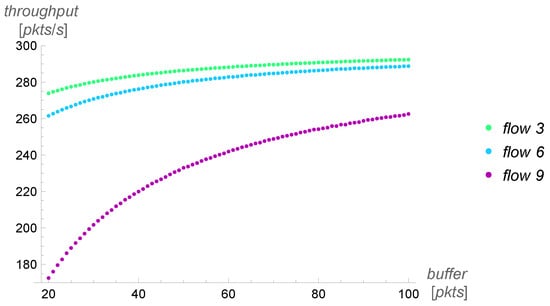
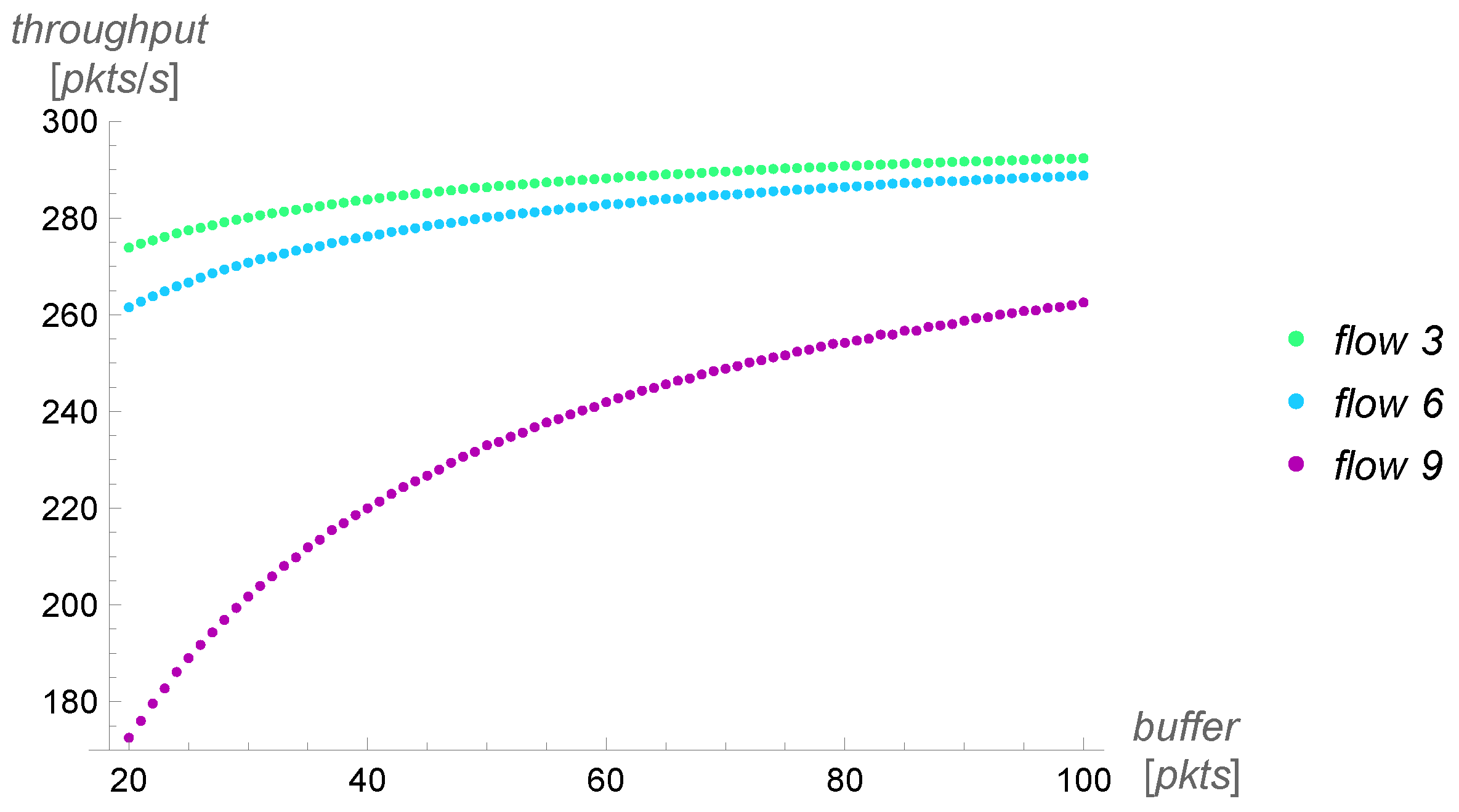
In Figure 7, the simulated throughput of flows 3, 6, and 9 is shown as a function of buffer size. All three flows have the same arrival rate of 300 pkts/s but differ in the variability of their interarrival times, ranging from the least variable flow 3 to the most variable flow 9. (We are back in the original flow parameterization, i.e., (55)–(63)).

As seen in Figure 7, the variability of a flow has a tremendous impact on throughput, especially when the buffer is small or moderate. For instance, when $K=20$, two flows with the same arrival rate may have throughput values as different as 172.5 and 273.9 pkts/s.

We may now return to the accuracy of predictions offered by Theorem 1. In all the previous results, a highly variable service (transmission) time was used. Assume now that the transmission time is constant. In

Table 7. Simulated and derived throughput for all flows. $K=20$, $\rho =1$, constant service.

Flow Number	1	2	3	4	5	6	7	8	9
simulated throughput [pks/s]	97.0	194.0	291.1	93.9	186.1	278.3	64.9	123.0	180.9
derived throughput [pks/s]	97.5	195.0	292.4	92.4	183.1	273.5	61.2	120.6	181.2
relative error	0.5%	0.5%	0.5%	1.6%	1.6%	1.7%	5.7%	2.0%	0.2%

, results for a buffer of 20 packets are shown;

Table 8. Simulated and derived throughput for all flows. $K=50$, $\rho =1$, constant service.

Flow Number	1	2	3	4	5	6	7	8	9
simulated throughput [pks/s]	98.5	196.9	295.4	97.0	193.1	289.0	82.1	161.0	239.5
derived throughput [pks/s]	99.0	198.0	297.0	96.9	193.1	289.2	81.2	160.8	240.5
relative error	0.5%	0.6%	0.5%	0.1%	0.0%	0.1%	1.1%	0.1%	0.4%

presents results for a buffer of 50 packets, while

Table 9. Simulated and derived throughput for all flows. $K=100$, $\rho =1$, constant service.

Flow Number	1	2	3	4	5	6	7	8	9
simulated throughput [pks/s]	99.2	198.3	297.6	98.3	196.3	293.9	90.3	178.3	266.5
derived throughput [pks/s]	99.5	199.0	298.5	98.5	196.6	294.6	90.0	178.7	267.5
relative error	0.3%	0.4%	0.3%	0.2%	0.2%	0.2%	0.4%	0.3%	0.4%

shows results for a buffer of 100 packets.

Table 7 ought to be considered in comparison with Table 2, which uses the same parameters except for the transmission time distribution. As observed, the less variable service time reduces the maximum error from 7.5% in Table 2 to 5.7% in Table 7. Moreover, the error for the majority of flows is also significantly smaller in Table 7 than in Table 2. Similarly, Table 8 ought to be considered in comparison with Table 3, differing only in the transmission time distribution. The maximum error in Table 8 is 1.1%, compared with 2.1% in Table 3. Then, Table 9 ought to be considered in comparison with Table 4. The maximum error in Table 9 is 0.4%, while in Table 4 it is 0.5%.

Moreover, when comparing Table 7 with Table 2, Table 8 with Table 3, and Table 9 with Table 4, it becomes clear that a reduction in the variance of the service time increases per-flow throughput for every specific flow, and every specific buffer size.

Finally, similarly to the case of gamma service, enlarging the buffer leads to an increase in per-flow throughput–see Table 7, Table 8 and Table 9 for a comparison across individual flows.

In Figure 8, the simulated and derived per-flow throughput is shown for buffer sizes ranging from 20 to 100 packets, while Figure 9 presents the corresponding relative errors. Figure 8 and Figure 9 were obtained assuming a constant service time and should be compared with Figure 3 and Figure 4, which were obtained for highly variable service times.

As seen in Figure 8 and Figure 9, the error decreases monotonically with increasing buffer size for all flows, except for flow 9, for which it remains close to zero across all buffer sizes.

In Figure 10, the simulated and derived per-flow throughput is shown for system loads varying from 0.1 to 1, while Figure 11 presents the corresponding relative errors. (Variable load was obtained by scaling the constant service time). Figure 10 and Figure 11 should be compared with Figure 5 and Figure 6, respectively.

As observed in Figure 10 and Figure 11, in the case of constant service time, the error also does not vary monotonically with $\rho$. Its maximum values occur around $\rho =0.9$–$0.95$, depending on the flow.

In the next set of results, the accuracy of predictions from Theorem 1 when the number of flows is 90 and 900 is tested.

Specifically, in the scenario with 90 flows, 10 flows of type (55), 10 flows of type (56), 10 flows of type (57), and so on, are used. This gives a total arrival rate of $\lambda$ = 18,000 pkts/s. The service time is again gamma-distributed with parameters $\alpha =0.25$ and $\theta =0.0002222222$, i.e., scaled to provide a service rate of 18,000 pkts/s ($\rho =1$), with $CV=2$.

Similarly, in the scenario with 900 flows, 100 flows of type (55), 100 flows of type (56), and so on, are used. Hence, $\lambda$ = 180,000 pkts/s. The service time is gamma with the same $\alpha$ and $\theta =0.00002222222$, i.e., scaled to a service rate of 180,000 pkts/s, while preserving $CV=2$ and $\rho =1$.

The results for the most demanding case–a very small buffer of 20 packets–are shown in

Table 10. Simulated and derived throughput in scenario with 90 flows. $K=20$, $\rho =1$, gamma service with $CV=2$.

Flow Number	1–10	11–20	21–30	31–40	41–50	51–60	61–70	71–80	81–90
simulated throughput [pks/s]	88.6	177.2	265.8	87.0	172.7	257.9	77.7	143.0	203.0
derived throughput [pks/s]	89.8	179.6	269.4	87.6	173.7	259.1	75.3	137.5	194.9
relative error	1.4%	1.4%	1.4%	0.7%	0.6%	0.5%	3.1%	3.8%	4.0%

and

Table 11. Simulated and derived throughput in scenario with 900 flows. $K=20$, $\rho =1$, gamma service with $CV=2$.

Flow Number	1–100	101–200	201–300	301–400	401–500	501–600	601–700	701–800	801–900
simulated throughput [pks/s]	88.8	177.6	266.3	88.4	176.1	263.4	87.0	170.4	250.8
derived throughput [pks/s]	89.8	179.6	269.4	89.3	177.9	266.1	87.6	171.3	251.7
relative error	1.1%	1.1%	1.2 %	1.0%	1.0%	1.0%	0.7%	0.5%	0.4%

, for 90 and 900 flows, respectively. These should be compared with the results in Table 2, obtained for 9 flows of the same types with other parameters unchanged. As observed, the maximum error is 4% in Table 10 and 1.2% in Table 11, compared with 7.5% in Table 2.

This result could have been expected. In the simplified model of Section 3, on which Theorem 1 is based, the limiting theorem is applied to the background traffic. Therefore, the simplified model better approximates the background traffic as the number of flows increases. And, vice versa, it may lead to substantial errors with a small number of flows.

The final scenario will be devoted to a stress test of the simplified model, to check how much its accuracy can deteriorate. Specifically, a very small buffer will be assumed (10 packets), accompanied by very few flows (3 flows), a very high diversity of flow rates (10:90:1700 pkts/s), very high variability of interarrival times ($C{V}_1=C{V}_2=C{V}_3=5$), and very high variability of service times ($CV=4$). Specifically, the following MAP matrices will be exploited:

$${\mathbf{D}}_0^1=\left[\begin{array}{cc}\hfill -0.7621& \hfill 0\\ \hfill 0& \hfill -993.2581\end{array}\right],{\mathbf{D}}_1^1=\left[\begin{array}{cc}\hfill 0.0575& \hfill 0.7045\\ \hfill 74.9893& \hfill 918.2688\end{array}\right],$$

(73)

$${\mathbf{D}}_0^2=\left[\begin{array}{cc}\hfill -6.8587& \hfill 0\\ \hfill 0& \hfill -8939.3230\end{array}\right],{\mathbf{D}}_1^2=\left[\begin{array}{cc}\hfill 0.5179& \hfill 6.3409\\ \hfill 674.9039& \hfill 8264.4191\end{array}\right],$$

(74)

$${\mathbf{D}}_0^3=\left[\begin{array}{cc}\hfill -129.5536& \hfill 0\\ \hfill 0& \hfill -168853.8787\end{array}\right],{\mathbf{D}}_1^3=\left[\begin{array}{cc}\hfill 9.7818& \hfill 119.7718\\ \hfill 12748.1844& \hfill 156105.6943\end{array}\right],$$

(75)

together with gamma service with parameters $\alpha =0.0625$ and $\theta =0.0088888888$.

The results are shown in

Table 12. Simulated and derived throughput in the stress-test scenario with 3 flows of rate proportions 10:90:1700, $K=10$, $\rho =1$ and gamma service with $CV=4$.

Flow Number	1	2	3
simulated throughput [pks/s]	7.2	48.4	749.2
derived throughput [pks/s]	5.8	37.3	746.0
relative error	19.4%	22.9%	0.4%

. As can be seen, the maximum error is now 22.9%, which is perhaps unacceptable in most applications. However, this outcome should be considered in light of two key factors.

Firstly, such parameterization is very unrealistic in the networking context. Specifically, it is unlikely that such a small buffer is used in a real networking device. It is also very unlikely that all the flows have such high variability of the interarrival time (with a standard deviation five times greater than the mean interarrival time). It is even less likely that the service time distribution has $CV=4$. For instance, in a typical IP network, packet sizes vary between 40 and 1500 bytes only. Hence, the greatest achievable coefficient of variation is far less than $CV=4$ (consider a 50/50 split between minimum and maximum packet sizes as the worst case).

Secondly, and most importantly, there is no need to use the simplified model in the case of very few flows and a small buffer. In such a case, it is possible to solve the full model of Section 3, because it involves matrices of reasonable size. For instance, in the stress-test scenario, these matrices would have sizes of only $88\times 88$.

7. Conclusions and Future Work

In the paper, the per-flow throughput of a FIFO buffer fed by complex traffic consisting of many flows with different statistical properties, was studied. Using a simplification based on a limiting theorem, formulae for per-flow throughput and loss ratio were derived (Theorem 1).

Due to the complexity of the model, it is practically impossible to prove rigorous error bounds for these formulae with respect to the full model, as functions of the model parameters.

Hence, the accuracy of the approximate results offered by Theorem 1 was tested in numerous demanding scenarios, involving flows with diversified rates and proportions, interarrival time variability, various buffer sizes, different system loads, three transmission time distributions, and four numbers of flows: 3, 9, 90, and 900.

The maximum error produced by Theorem 1 was about 8% in all scenarios with 9 or more flows, a buffer of at least 20 packets, and bandwidth consumed by any single flow no greater than 25%.

The maximum error dropped quickly with the buffer size, to 2.1% for $K=50$ and 0.5% for $K=100$. It also dropped with the number of flows, to 4% for $N=90$ and 1.2% for $N=900$, even when a small buffer was used.

In a stress-test scenario, with only 3 highly variable flows, one of which is consuming most of the bandwidth, a buffer of 10 packets, and highly variable service time, the maximum error was 23%, which is perhaps too much for most applications. This scenario was, however, highly unrealistic with respect to the very small buffer and extreme variability of the service time. Furthermore, it was argued that scenarios with a low number of flows can be solved numerically using the full model, with no approximations involved.

Finally, the impact of all system parameters on per-flow throughput was examined experimentally. In particular, it was observed that per-flow throughput decreases with increasing the variability of the interarrival time within the flow, decreases with increasing the variability of the service time, and increases with enlarging the buffer.

Future research directions may explore distributions of per-flow queueing delay or per-flow queue length, i.e., number of packets from each flow stored in the buffer at an arbitrary time. It may also consist of a comparison of the model with experiment results based on trace-fitted or real traffic data.

References

- Chydzinski, A.; Adamczyk, B. Per-flow Packet Loss Ratios Induced by an Overflowed Buffer. In Proceedings of the 17th International Conference on Web Information Systems and Technologies (WEBIST 2021), Online, 26–28 October 2021; pp. 621–628. [Google Scholar]
- Coates, M.; Nowak, R. Network loss inference using unicast end-to-end measurement. In Proceedings of the ITC Specialist Seminar on IP Traffic Measurement, Modeling and Management, Monterey, CA, USA, 18–20 September 2000. [Google Scholar]
- Duffield, N.G.; Presti, F.L.; Paxson, V.; Towsley, D. Inferring link loss using striped unicast probes. In Proceedings of the Twentieth Annual Joint Conference of the IEEE Computer and Communications Society, Anchorage, AK, USA, 22–26 April 2001; pp. 915–923. [Google Scholar]
- Benko, P.; Veres, A. A passive method for estimating end-to-end TCP packet loss. In Proceedings of the Global Telecommunications Conference, Taipei, Taiwan, 17–21 November 2002; pp. 2609–2613. [Google Scholar]
- Sommers, J.; Barford, P.; Duffield, N.; Ron, A. Improving accuracy in end-to-end packet loss measurement. Comput. Commun. Rev. 2005, 35, 157–168. [Google Scholar] [CrossRef] [Scilit]
- Sommers, J.; Barford, P.; Duffield, N.; Ron, A. A geometric approach to improving active packet loss measurement. IEEE/ACM Trans. Netw. 2008, 16, 307–320. [Google Scholar] [CrossRef] [Scilit]
- Lan, H.; Ding, W.; Zhang, Y. Strengthening packet loss measurement from the network intermediate point. KSII Trans. Internet Inf. Syst. 2019, 13, 5948–5971. [Google Scholar] [CrossRef] [Scilit]
- Kleinrock, L. Queueing Systems: Theory; John Wiley and Sons: New York, NY, USA, 1975. [Google Scholar]
- Takagi, H. Queueing Analysis-Finite Systems; North-Holland: Amsterdam, The Netherlands, 1993. [Google Scholar]
- Baiocchi, A.; Blefari-Melazzi, N. Steady-state analysis of the MMPP/G/1/K queue. IEEE Trans. Commun. 1992, 41, 531–534. [Google Scholar] [CrossRef]
- Chydzinski, A.; Adamczyk, B. Transient and stationary losses in a finite-buffer queue with batch arrivals. Math. Probl. Eng. 2012, 2012, 326830. [Google Scholar] [CrossRef] [Scilit]
- Banik, A.D.; Chaudhry, M.L. Efficient Computational Analysis of Stationary Probabilities for the Queueing System BMAP/G/1/N with or Without Vacation(s). Inf. J. Comput. 2017, 29, 140–151. [Google Scholar] [CrossRef] [Scilit]
- Dudin, A.N.; Klimenok, V.I.; Vishnevsky, V.M. The Theory of Queuing Systems with Correlated Flows; Springer: Cham, Swizterland, 2020. [Google Scholar]
- Cidon, I.; Khamisy, A.; Sidi, M. Analysis of packet loss processes in high-speed networks. IEEE Trans. Inf. Theory 1993, 39, 98–108. [Google Scholar] [CrossRef] [Scilit]
- Bratiychuk, M.; Chydzinski, A. On the loss process in a batch arrival queue. Appl. Math. Model. 2009, 33, 3565–3577. [Google Scholar] [CrossRef] [Scilit]
- Ancker, C.J.; Gafarian, A.V. Queuing with Multiple Poisson Inputs and Exponential Service Times. Oper. Res. 1961, 9, 321–327. [Google Scholar] [CrossRef] [Scilit]
- Habib, M.E.L. Queues with Multiple Poisson Inputs & Erlang Service Times. Science 1989, I, 231–239. [Google Scholar]
- Stanford, D.; Fischer, W. The interdeparture-time distribution for each class in the ∑i Mi/Gi/1 queue. Queueing Syst. 1989, 4, 179–191. [Google Scholar] [CrossRef] [Scilit]
- Nikolov, A.V. Finite capacity queue with multiple Poisson arrivals and generally distributed service times. Int. J. Appl. Math. 2013, 26, 233–240. [Google Scholar] [CrossRef] [Scilit]
- Holtzman, J.M. Mean Delays of Individual Streams into a Queue: The ∑GIi/M/1 Queue. In Applied Probability-Computer Science: The Interface Volume 1; Progress in Computer Science; Disney, R.L., Ott, T.J., Eds.; Birkhäuser: Boston, MA, USA, 1982; Volume 2. [Google Scholar]
- Albin, L.S. Delays for Customers from Different Arrival Streams to a Queue. Manag. Sci. 1986, 32, 329–340. [Google Scholar] [CrossRef] [Scilit]
- Fischer, W.; Stanford, D. Approximations for the per-class waiting time and interdeparture time in the ∑iGIi/GIi/1 queue. Perform. Eval. 1992, 14, 65–78. [Google Scholar] [CrossRef] [Scilit]
- Whitt, W. Towards better multi-class parametric-decomposition approximations for open queueing networks. Ann. Oper. Res. 1994, 48, 221–248. [Google Scholar] [CrossRef] [Scilit]
- Peshkova, I.; Morozov, E.; Pagano, M. Regenerative Analysis and Approximation of Queueing Systems with Superposed Input Processes. Mathematics 2024, 12, 2202. [Google Scholar] [CrossRef] [Scilit]
- Courcoubetis, C.; Weber, R. Buffer overflow asymptotics for a buffer handling many traffic sources. J. Appl. Probab. 1996, 33, 886–903. [Google Scholar] [CrossRef] [Scilit]
- Likhanov, N.; Mazumdar, R. Cell loss asymptotics in buffers fed with a large number of independent stationary sources. In Proceedings of the Seventeenth Annual Joint Conference of the IEEE Computer and Communications Societie, San Francisco, CA, USA, 29 March–2 April 1998; Volume 1, pp. 339–346. [Google Scholar]
- Likhanov, N.; Mazumdar, R. Cell loss asymptotics in buffers fed by heterogeneous long-tailed sources. In Proceedings of the Nineteenth Annual Joint Conference of the IEEE Computer and Communications Societies, Tel Aviv, Israel, 26–30 March 2000; Volume 1, pp. 173–180. [Google Scholar]
- Ghiassi-Farrokhfal, Y.; Ciucu, F. On the impact of finite buffers on per-flow delays in FIFO queues. In Proceedings of the 2012 24th International Teletraffic Congress (ITC 24), Krakow, Poland, 4–7 September 2012; pp. 1–8. [Google Scholar]
- Chydzinski, A. Queue Size in a BMAP Queue with Finite Buffer. In Next Generation Teletraffic and Wired/Wireless Advanced Networking; Lecture Notes in Computer Science; Springer: Berlin/Heidelberg, Germany, 2006; Volume 4003, pp. 200–210. [Google Scholar]
- Salvador, P.; Valadas, R.; Pacheco, A. Multiscale Fitting Procedure Using Markov Modulated Poisson Processes. Telecommun. Syst. 2003, 23, 123–148. [Google Scholar] [CrossRef] [Scilit]
- Salvador, P.; Pacheco, A.; Valadas, R. Modeling IP traffic: Joint characterization of packet arrivals and packet sizes using BMAPs. Comput. Netw. 2004, 44, 335–352. [Google Scholar] [CrossRef] [Scilit]
- Casale, G.; Zhang, E.Z.; Smirni, E. Trace data characterization and fitting for Markov modeling. Perform. Eval. 2010, 67, 61–79. [Google Scholar] [CrossRef] [Scilit]
- Buchholz, P. An EM-Algorithm for MAP Fitting from Real Traffic Data. In Computer Performance Evaluation Modelling Techniques and Tools; Lecture Notes in Computer Science; Kemper, P., Sanders, W.H., Eds.; Springer: Berlin/Heidelberg, Germany, 2003; Volume 2794, pp. 218–236. [Google Scholar]
- Klemm, A.; Lindemann, C.; Lohmann, M. Modeling IP traffic using the batch Markovian arrival process. Perform. Eval. 2003, 54, 149–173. [Google Scholar] [CrossRef] [Scilit]
- Daley, D.J.; Vere-Jones, D. An Introduction to the Theory of Point Processes, Volume II: General Theory and Structure, 2nd ed.; Springer: New York, NY, USA, 2008. [Google Scholar]
- Chydzinski, A. Time to reach buffer capacity in a BMAP queue. Stoch. Model. 2007, 23, 195–209. [Google Scholar] [CrossRef] [Scilit]
- Available online: https://omnetpp.org/ (accessed on 20 March 2026).
Disclaimer/Publisher’s Note: The statements, opinions and data contained in all publications are solely those of the individual author(s) and contributor(s) and not of MDPI and/or the editor(s). MDPI and/or the editor(s) disclaim responsibility for any injury to people or property resulting from any ideas, methods, instructions or products referred to in the content. |
© 2026 by the author. Published by MDPI on behalf of the International Institute of Knowledge Innovation and Invention. Licensee MDPI, Basel, Switzerland. This article is an open access article distributed under the terms and conditions of the Creative Commons Attribution (CC BY) license.