
Article

An Intelligent Decision-Support Framework Based on Fuzzy BWM–TOPSIS with Interdependent Criteria for Alternative Selection in Complex Construction Projects

by
Luong Duc Long
1,2,*,
Vo Thi Dinh Khanh
1,2,
Nguyen Quang Trung
3 and
Truong Ngoc Son
1,2
1
Faculty of Civil Engineering, University of Technology (HCMUT), No. 268 Ly Thuong Kiet Street, Dien Hong Ward, Ho Chi Minh City 700000, Vietnam
2
Vietnam National University Ho Chi Minh City (VNU-HCM), Linh Xuan Ward, Ho Chi Minh City 700000, Vietnam
3
Faculty of Project Management, University of Science and Technology (DUT), The University of Danang, 54 Nguyen Luong Bang Street, District Lien Chieu, Da Nang City 550000, Vietnam
*
Author to whom correspondence should be addressed.
Appl. Syst. Innov. 2026, 9(6), 108; https://doi.org/10.3390/asi9060108
Submission received: 7 April 2026 / Revised: 21 May 2026 / Accepted: 25 May 2026 / Published: 26 May 2026
(This article belongs to the Special Issue AI-Driven Decision Support for Systemic Innovation)

Highlights

-
Proposing an interdependency-aware fuzzy BWM for complex multi-criteria decision making.
-
Modeling cross-criterion influences via fuzzy nonlinear optimization.
-
Preserving individual expert judgments within a transparent group decision-making process.
-
Implementing a reproducible framework for weighting and ranking alternatives.
-
Demonstrating applicability through a real-world infrastructure case study.

Abstract

This study proposes an intelligent decision-support framework for alternative selection in complex construction projects, where evaluation processes are affected by uncertainty, multiple decision-makers, and interdependent criteria. The framework integrates the fuzzy group best–worst method with fuzzy TOPSIS into a unified structure that explicitly captures cross-criterion influence effects. First, triangular fuzzy judgments from multiple experts are used to derive criterion weights, while interdependencies among criteria are represented through a fuzzy influence-intensity matrix and incorporated into fuzzy nonlinear optimization models. This process enables the systematic estimation of both independent and interdependency-adjusted criterion weights. Second, the resulting weights are used in a fuzzy ranking procedure to evaluate alternatives according to their relative closeness to fuzzy ideal solutions. To enhance transparency, reproducibility, and practical usability, the proposed method is implemented in Python as an automated computational workflow for decision analysis. Its applicability is demonstrated through a real-world case study on access platform system selection for mechanical, electrical, and plumbing installation in an airport terminal subject to safety, productivity, workspace, and elevation-related constraints. The results show that explicitly modeling criterion interdependencies provides a more realistic evaluation structure and enhances the robustness and reliability of alternative selection in complex construction management contexts.

1. Introduction

The success of construction projects largely depends on the efficiency of labor crews and the effective management of supporting resources. Among these resources, scaffolding systems constitute a critical category of temporary structures, providing essential access and working platforms that facilitate task execution and significantly influence overall project performance [1,2]. Scaffolding systems are temporary structures whose layouts and locations change over the course of construction. As it is shared by multiple trades, its interaction with different construction activities often leads to coordination issues that only become apparent during execution [3]. These challenges are particularly pronounced in today’s large-scale and complex construction projects. Various scaffolding systems, including scissor lifts, vertical lifts, telescopic lifts, and modular scaffolding, can be selected to accommodate complex site conditions. In addition, onsite construction operations such as bolting and welding require suitable scaffolding systems to ensure adequate support.
Construction work requires suitable working areas to be carried out safely and efficiently. The positions, sizes, and shapes of these working areas change over time in three-dimensional space, depending on project design details and construction schedules. This dynamic characteristic is particularly pronounced in modern construction projects with high levels of complexity and spatial constraints [4]. Consequently, scaffolding systems and work platforms must be properly planned and positioned to adapt to these changes. Failure to account for workspace dynamics can reduce productivity, increase safety risks, and result in inefficient use of temporary facilities.
The selection of appropriate temporary facilities, particularly scaffolding systems, plays a critical role in controlling costs and enhancing the productivity and safety of construction workers [5]. Nevertheless, conventional manual planning approaches for scaffolding systems are often inefficient and prone to errors [2]. Determining the most appropriate scaffolding type and configuration therefore constitutes a complex planning and decision-making problem. This task requires the integrated assessment of diverse quantitative and qualitative criteria, including construction productivity, safety performance, cost efficiency, construction duration, and other sustainability-related objectives. The difficulty of this selection process is further exacerbated in modern construction projects characterized by high levels of complexity and uncertainty. To improve planning efficiency, there is a clear need for an automated decision-support model capable of systematically incorporating these criteria within complex project environments and assisting planners in selecting suitable scaffolding systems.
Complex construction projects, such as airport developments, increasingly involve non-standard and non-routine work conditions, particularly in the use of temporary structures including scaffolding and access platforms. The selection of scaffolding systems is typically performed under stringent resource constraints—such as limited labor availability, restricted workspace, and tight construction schedules—combined with uncertainty arising from variable labor productivity, safety requirements, access demands, and load-bearing requirements. These challenges are especially evident in scaffolding selection for MEP installation beneath terminal roof ceilings, where spatial conflicts among MEP systems, limited ceiling-level accessibility, operational constraints within active terminals, and variability in work sequencing and trade coordination are frequently encountered. Consequently, project stakeholders must simultaneously balance multiple, often conflicting objectives, including schedule, cost, safety, and sustainability.
In airport projects, scaffolding systems are frequently affected by design changes, trade coordination conflicts, safety inspections, and unforeseen site conditions, substantially increasing uncertainty in evaluating alternatives. As a result, scaffolding system selection represents a complex multi-criteria decision-making (MCDM) problem that conventional deterministic or purely probabilistic methods cannot adequately address, particularly under limited historical data and reliance on expert judgment. Under such conditions, fuzzy set theory offers an effective framework for representing imprecise and linguistic expert assessments and for systematically integrating schedule, cost, safety, sustainability, and constructability criteria under uncertainty [6].
Despite these challenges, existing studies have not yet provided a comprehensive decision-support framework for scaffolding system selection that simultaneously accounts for criterion interdependencies, nonlinear uncertainty, and practical implementability in complex construction environments.
To address this gap, this study aims to develop an interdependency-aware fuzzy group decision-support framework for selecting access platform systems in complex construction projects. The specific objectives are (1) to formulate a fuzzy group best–worst method with interdependency (FIDBWM) that simultaneously captures expert uncertainty, group decision making, and cross-criterion influence effects; (2) to derive both independent and interdependency-adjusted criterion weights within a unified fuzzy nonlinear optimization structure; (3) to integrate the resulting weights with fuzzy TOPSIS for ranking alternative access platform systems under uncertain performance assessments; (4) to implement the proposed framework in a Python-based computational workflow; and (5) to demonstrate and validate the framework through a real-world airport terminal case study, comparative fuzzy VIKOR analysis, expert verification, and sensitivity analysis.

2. Literature Review

2.1. Decision-Support Systems and Modeling Approaches for Scaffolding

Existing studies indicate that research on decision-support systems and modeling approaches for scaffolding planning remains relatively limited. For example, Fang et al. [7] presented an AHP-based framework incorporating expert judgment for scaffolding assessment and selection (bamboo and metal scaffolding), revealing that metal scaffolding outperforms bamboo scaffolding overall. To address the need for more comprehensive decision making, subsequent studies sought to incorporate additional criteria and expert knowledge into scaffolding planning practices. Jin et al. [8] developed an automated optimization framework that integrates key criteria of scaffolding systems to concurrently maximize task coverage, enhance mechanical piping productivity, and minimize scaffolding labor input.
Kim and Fischer [9] formalized a taxonomy of temporary structures and established relationships between construction activity characteristics and scaffolding types, leading to a heuristic-based selection process to support engineering decisions. Kim et al. [10] further developed a semi-automated scaffolding planning generator (SPG) to select suitable scaffolding systems based on the geometric and operational features of construction activities. Kim et al. [11] proposed a comprehensive decision-making framework that evaluates scaffolding plans in terms of safety, cost, and duration by combining quantitative analysis with expert judgment. Recently, Espinoza et al. [12] investigated the use of the choosing by advantages (CBA) method for scaffolding selection in construction projects, highlighting the limitations of experience-based decision making. The results show that CBA improves transparency and collaboration in the scaffolding selection process, though practical implementation barriers remain.
However, existing scaffolding planning approaches largely rely on conventional MCDM techniques that assume criteria independence and deterministic evaluations. Such assumptions limit their ability to capture both the inherent uncertainty of expert judgments and the interdependencies among evaluation criteria, which are characteristic of complex construction projects. Consequently, a clear research gap exists for the development of an advanced fuzzy MCDM–based decision-support model that explicitly incorporates criterion interdependencies, allowing for more realistic and reliable scaffolding selection under uncertainty.

2.2. Applications of Multi-Criteria Decision-Making Methods in the Construction Industry

Construction is a decision-intensive field in which effective decision making is critical to project success. The sector is characterized by activities that involve numerous and often conflicting factors, making comprehensive management challenging [13]. Accordingly, multi-criteria decision-making (MCDM) techniques have been increasingly used in construction decision making to address conflicting criteria by jointly considering economic, environmental, and social factors [13].
Previous studies demonstrate that MCDM methods are particularly effective in addressing uncertainty, subjectivity, and trade-offs inherent in construction-related decisions. Fayek [14] provided a comprehensive review of fuzzy hybrid approaches in construction applications, highlighting their effectiveness in solving optimization problems, multicriteria decision-making tasks, and simulation-based analyses.
Several researchers have applied integrated MCDM frameworks to specific construction decision contexts. In the context of supplier evaluation, Wang et al. [15] integrated AHP with Grey relational analysis to develop a robust supplier selection framework tailored to construction projects, while Zhao et al. [16] proposed an AHP-based approach for prefabrication projects to hierarchically prioritize evaluation criteria and derive relative supplier scores.
Sustainability-oriented decision making has also received considerable attention; Mathiyazhagan et al. [17] developed a three-phase evaluation model using the best–worst method (BWM) and the fuzzy technique for order of preference by similarity to ideal solution (TOPSIS) to support sustainable construction material selection. Amorocho and Harmann [18] proposed a TOPSIS-driven decision framework for selecting renovation solutions for residential buildings, which was successfully validated through two real-world case studies.

2.3. The Best–Worst Method (BWM) in MCDM

The best–worst method (BWM) provides an efficient and consistent mechanism for determining criterion weights by using pairwise comparisons between the most and least influential criteria [19,20]. The method has received considerable attention in recent years, leading to numerous empirical applications [21,22,23], methodological extensions [24,25], and fuzzy variants designed to address uncertainty in expert evaluations [26,27,28,29,30]. Fuzzy logic is especially valuable in construction and infrastructure projects due to the prevalence of linguistic judgments and incomplete information [31,32].
Recent developments include Z-number-based BWM [33], fuzzy programming-based TF-BWM [26], intuitionistic fuzzy extensions [34], interval-valued and fuzzy–rough models [30], and hybrid frameworks combining BWM with VIKOR, MARCOS, and other MCDM techniques [35,36,37,38,39]. Applications in supplier selection, logistics, safety assessment, and sustainability planning further demonstrate BWM’s adaptability [40].
Nevertheless, many BWM applications depend on optimization software, such as LINGO or Excel Solver, which may limit scalability, transparency, and automation. Although a recent Python-based fuzzy BWM–TOPSIS model has improved procedural efficiency in contractor selection [41], it does not incorporate interdependencies among criteria.
Despite its popularity and reliability, the best–worst method (BWM) typically assumes that decision criteria are independent, whereas in most real-world decision-making problems, criteria are inherently interdependent. To address this limitation, Tavana et al. [37] proposed a generalized form of the BWM (GBWM) that accounts for both criterion interdependencies and the intensity of their mutual influences when deriving relative influence-intensity weights.

2.4. BWM-Based Modeling of Influences Among Interrelated Criteria

Although the traditional best–worst method (BWM) assumes independence among criteria and therefore yields independent weights, several studies have sought to relax this assumption by integrating BWM with causal and network-oriented techniques. Specifically, Yazdi et al. (2020) [42] developed an integrated DEMATEL–BWM framework combined with Bayesian networks to model dependency relationships and influence intensity among criteria, and demonstrated its applicability through a safety management case study in the high-tech industry.
Similarly, Tavana et al. (2021) [43] proposed a hybrid BWM–WINGS framework, in which the weighted influence nonlinear gauge system (WINGS) captures feedback effects and mutual influences among interrelated criteria through ideographic causal maps. Liang et al. (2023) [44] proposed an integration of the Choquet integral and BWM, highlighting the feasibility of explicitly modeling interaction effects within the weighting procedure. Govindan et al. (2022) [45] combined BWM with the decision-making trial and evaluation laboratory (DEMATEL) to model cause–effect relationships among criteria, allowing both direct and indirect influence structures to be identified in complex decision-making systems.
More recently, Tavana et al. (2023) [37] introduced the general best–worst method (GBWM), which represents a significant advancement over the classical BWM by directly embedding criterion interdependencies into the optimization model, thereby eliminating the need for auxiliary causal techniques. By doing so, GBWM effectively overcomes the independence assumption inherent in the traditional BWM. Building upon this solid foundation, extensions that incorporate fuzzy representations and group decision making can further enhance the applicability of GBWM in real-world contexts characterized by uncertainty and heterogeneous expert judgments.
In construction decision-making problems, uncertainty is further amplified by project-specific conditions, expert subjectivity, and complex interdependencies among criteria, while decisions are typically made in group settings involving multiple experts or multiple stakeholders. Despite these characteristics, the joint consideration of uncertainty, criterion interdependencies, and the systematic aggregation of heterogeneous judgments from multiple experts has not yet been adequately addressed within the existing GBWM framework. Moreover, as the number of experts increases, the associated fuzzy nonlinear constraints grow rapidly in both scale and complexity, highlighting the need for automated modeling and solution procedures. To bridge this gap, this study develops a fuzzy interdependency-aware group best–worst method, FIDBWM, integrated with fuzzy TOPSIS and supported by a computational program that automatically generates and efficiently solves fuzzy nonlinear constraint systems. The proposed framework simultaneously captures uncertainty, interdependent criterion structures, and collective expert judgments in complex construction decision-making environments.

2.5. Positioning Relative to DEMATEL-Based and GBWM-Based Interdependency Models

A number of hybrid MCDM studies have incorporated interdependent criteria using DEMATEL, ANP, BWM, TOPSIS, and related network-based structures. In DEMATEL-based frameworks, interdependencies are commonly represented through a direct-relation matrix, which is normalized and transformed into a total-relation matrix to identify causal influence patterns, prominence, and net cause-effect relationships. When DEMATEL is combined with TOPSIS, DEMATEL is typically used to derive interrelationships or criterion weights, while TOPSIS is subsequently used for alternative ranking.
The present study differs from DEMATEL-based dependency modeling in both purpose and modeling logic. DEMATEL-based approaches are primarily designed to reveal causal structures and influence directions among factors. In contrast, the proposed FIDBWM framework uses interdependency information as part of a BWM-compatible weighting mechanism. The objective is not primarily to construct a cause-and-effect diagram, but to obtain both independent and interdependency-adjusted fuzzy weights that can be directly used in the subsequent fuzzy TOPSIS ranking stage.
The proposed approach (FIDBWM) also differs from conventional GBWM extensions. GBWM provides an important foundation for incorporating criterion interdependency into the BWM structure. However, the present study extends this logic by simultaneously incorporating triangular fuzzy uncertainty, embedded group decision making, decision-maker-specific judgments, and automated Python-based solution of the fuzzy nonlinear constraint system. Therefore, the contribution is not merely the combination of existing tools, but rather the construction of a unified fuzzy group interdependency-aware weighting and ranking workflow for complex construction decisions. Table 1 summarizes the methodological positioning of the proposed FIDBWM–TOPSIS framework.

3. An Integrated FIDBWM–TOPSIS Framework for Decision-Making Under Criterion Interdependency and Uncertainty

The proposed FIDBWM–TOPSIS framework is theoretically grounded in four established methodological streams. First, the best–worst method provides a consistency-based mechanism for deriving criterion weights from best-to-others and others-to-worst comparisons [19,20]. Second, fuzzy BWM and group fuzzy decision making extend this logic to linguistic and uncertain expert judgments represented by triangular fuzzy numbers [27,38,41]. Third, interdependency-aware BWM and related network-based MCDM models demonstrate that criteria may influence one another and that such relationships can be incorporated into the weighting process rather than being ignored under an independence assumption [37,43]. Fourth, fuzzy TOPSIS and fuzzy VIKOR provide established ideal-solution and compromise-ranking mechanisms for evaluating alternatives under uncertainty [47,48,49,50,51,52]. Building on these foundations, the present study formulates FIDBWM–TOPSIS as a BWM-compatible fuzzy group extension that derives independent weights, propagates interdependency-adjusted weights, and connects the resulting weights to fuzzy alternative ranking within a traceable computational workflow.
This study integrates systematic factor identification with the development of a multi-criteria decision-making (MCDM) framework to support the selection of appropriate scaffolding and access platform systems in complex construction projects. Potential technical, economic, safety, constructability, and sustainability-related factors influencing scaffolding performance were first identified through an extensive literature review, expert consultations, and a structured survey involving practitioners engaged in large-scale and complex construction projects.
To ensure contextual relevance, a project-specific expert panel was subsequently established for the airport MEP installation case. This panel reviewed, refined, and consolidated the candidate factors, resulting in nine key evaluation criteria considered essential for scaffolding and access platform selection under the specific project conditions. These finalized criteria formed the basis for developing an integrated MCDM framework that combines the fuzzy group best–worst method with interdependency (FIDBWM) for fuzzy weight determination and explicit modeling of criterion interdependencies, together with fuzzy TOPSIS for ranking alternative scaffolding systems.
Within the proposed framework, the FIDBWM method determines the relative importance of evaluation criteria based on expert judgments expressed in linguistic terms. These judgments are represented using triangular fuzzy numbers (TFNs) to capture epistemic uncertainty. Criterion interdependencies are explicitly incorporated into the weighting process, enabling relationships among criteria to be represented. Subsequently, fuzzy TOPSIS is applied to rank scaffolding and access platform alternatives according to their relative closeness to the ideal solution under fuzzy conditions, thereby providing a transparent and practically implementable decision-support tool for complex construction environments.

3.1. Modeling Uncertainty Using Fuzzy Sets

Fuzzy set theory [31] is adopted to capture uncertainty and heterogeneity in group decision making for construction–MEP projects. Expert judgments expressed through linguistic terms (e.g., safety level or cost efficiency) are modeled using triangular fuzzy numbers (TFNs) with lower, modal, and upper bounds. These TFNs are consistently applied in both criteria weighting via fuzzy BWM and alternative evaluation using fuzzy TOPSIS. The linguistic scales employed are reported in Table 2 and Table 3. This approach enables systematic aggregation of multiple experts’ subjective opinions and enhances the robustness of decision outcomes in complex and uncertain construction–MEP environments.
The detailed TFN operations and scalarization rules are provided in Appendix B.

3.2. Fuzzy Group BWM (FGBWM) Model Considering Interdependency and Uncertainty

In Stage 1, baseline criteria weights are derived using the fuzzy group best–worst method (FGBWM) under the assumption of mutual independence among criteria. Subsequently, Stage 2 refines these baseline weights by explicitly incorporating interdependency effects through fuzzy influence modeling, thereby yielding interdependency-adjusted criteria weights. This formulation extends the conventional FGBWM framework by simultaneously accounting for criteria interdependency and epistemic uncertainty in the weighting process.

3.2.1. Stage 1 (Implementing FGBWM and Calculating the Independent Criteria Weights)

Step 1. Criteria System—Define J essential criteria c r 1 , . . , c r j , , c r J , j = 1 , 2 , , J that are used to evaluate the performance of the alternatives.
Step 2. Fuzzy Comparative Evaluations—Conduct pairwise comparisons using TFNs for each D M ( k ) .
The model considers a group of K decision makers. Each decision maker D M ( k ) provides the following inputs:
  • v B x k ~ : Best-to-others (BO) fuzzy judgments expressed as triangular fuzzy numbers (TFNs), and v B x k ~ = ( v B x , 1 k ~ , . . , v B x , j k ~ , . . , v B x , J k ~ ).
  • v W x k ~ : Others-to-worst (OW) fuzzy judgments expressed as TFNs, and v W x k ~ = ( v 1 , W x k ~ , . . , v j , W x k ~ , . . , v J , W x k ~ ).
  • B x and W x : Indices of the best and worst criteria, respectively.
Step 3. Decision variables and constraints for determining the optimal weights without interdependency.
At this stage, the group fuzzy best–worst method (TFN-BWM) is employed to determine the baseline criteria weights under the assumption that no interdependencies exist among the criteria. The objective of this stage is to determine a common fuzzy weight vector whose components serve as the decision variables as follows:
w ~ = w 1 ~ , w 2 ~ , , w j ~ , . . , w J ~ ,
where each w j ~ = w j 1 , w j 2 , w j 3 is represented by a triangular fuzzy number.
Unlike conventional group decision-making approaches, the proposed model simultaneously incorporates all decision-makers into a unified nonlinear optimization framework. This formulation preserves the original uncertainty and heterogeneity inherent in expert opinions.
Fuzzy Best–Worst Consistency Constraints
These fuzzy ratio relationships are enforced through a deviation-minimization mechanism embedded within a nonlinear optimization framework. For each decision maker k, a deviation variable ξ D M k is introduced to quantify the maximum inconsistency between the derived fuzzy criteria weight ratios and the corresponding fuzzy best-to-others (BO) and others-to-worst (OW) judgments provided by that decision maker. Specifically, this deviation variable captures the largest absolute discrepancy between the computed fuzzy weight ratios and the expert-assessed fuzzy preference values.
Based on the fuzzy BWM consistency principle [27], which extends the original BWM pairwise comparison logic [19,20], the fuzzy ratio relationships between the derived fuzzy weights and the BO/OW judgments for each decision maker k are formulated through a deviation-minimization mechanism as follows:
w j = B x ~ w j ~ v B x , j k ~ ξ D M k ~ ,
w j ~ w j = W x ~ v j , W x k ~ ξ D M k ~ , j = 1 , , J ; k = 1 , , K
where w j ~ denotes the fuzzy weight of criterion j , while v B x , j k ~ and v j , W x k ~ denote the fuzzy best-to-others (BO) and others-to-worst (OW) preference judgments provided by decision maker k , respectively.
By minimizing a weighted aggregation of the deviation variables ξ D M k ~ across all decision makers, the proposed model seeks to minimize the maximum absolute deviations between the derived fuzzy weight ratios and the corresponding expert judgments. This optimization strategy ensures that the resulting fuzzy criteria weights are globally consistent with the collective assessments of all decision makers, while fully preserving the uncertainty and imprecision inherent in the original fuzzy input information. Consequently, the proposed formulation achieves internal consistency across heterogeneous expert evaluations.
To handle triangular fuzzy numbers (TFNs), the model applies the graded mean integration representation (GMIR) [27,38] to convert each fuzzy term w j ~ =   T F N w j 1 , w j 2 , w j 3 into a crisp value as follows:
GradMean w j ~ = 1 6 w j 1 + 4 w j 2 + w j 3  
To ensure proper normalization of fuzzy weights and to enhance the numerical stability of the fuzzy nonlinear programming model, the normalization scheme proposed by Wang et al. (2006) [53] is adopted. Specifically, the fuzzy weight vector w ~ is normalized by enforcing the following constraints [53]:
( j C r w j 2 = 1 ; w j 1 3 + j C r , j j 1 w j 1 1   a n d   w j 1 1 + j C r , j j 1 w j 3 1 )
These conditions ensure that the sum of the middle values equals one, while the lower and upper bounds satisfy complementary inequality constraints. Such normalization prevents the excessive expansion of fuzzy intervals, improves convergence behavior, and leads to more reliable and interpretable weighting results [53].
Step 4. Mathematical formulation for determining optimal weights using the FGBWM without interdependency.
At this stage, the optimization problem minimizes the overall fuzzy consistency deviation of the group decision-making model. For the group setting, the individual decision-maker deviation variables are aggregated into a single weighted scalar consistency objective. This structure extends the crisp group BWM formulation of Safarzadeh et al. [25] to a TFN-based fuzzy environment and follows the computational group fuzzy BWM–TOPSIS orientation of Long [41] as follows:
M i n ξ G e n e r a l = M i n ( C o e f W D M k = 1 ξ D M k = 1 + C o e f W D M k = 2 ξ D M k = 2 + + C o e f W D M k = K ξ D M k = K )
where ξ G e n e r a l is the aggregated group consistency deviation, ξ D M k = K denotes the maximum fuzzy consistency deviation of decision maker DM k , and C o e f W D M k = K is the corresponding decision-maker weighting coefficient, with
k = 1 K C o e f W D M k = 1
This formulation treats the model as a weighted scalar deviation-minimization problem while retaining the individual consistency contribution of each decision maker. It also clarifies that the objective function is a single scalar performance indicator, not a separate objective for each decision maker.
  s . t .   w j = B x ~ w j ~ v B x , j k ~ ξ D M k ~ w j ~ w j = W x ~ v j , W x k ~ ξ D M k ~ j = 1 J   G r a d M e a n w j ~ = j = 1 J   1 6 w j 1 + 4 w j 2 + w j 3 = 1 j C r w j 2 = 1 w j 1 3 + j C r , j j 1 w j 1 1 w j 1 1 + j C r , j j 1 w j 3 1 w j ~ = T F N w j 1 , w j 2 , w j 3 ; w j 1 w j 2 w j 3 ; w j 1 0 w h e r e j = 1 , 2 , , J   a n d   k = 1 , . . , K  
where ξ ~ D M k = ξ D M k , ξ D M k , ξ D M k and k = 1 , . . , K . It should be noted that a triangular fuzzy number (TFN) constraint w j = B x ~ w j ~ v B x , j k ~ ξ D M k ~ is equivalently represented by three component-wise scalar absolute-deviation constraints.
The resulting model constitutes a fuzzy nonlinear constrained optimization problem characterized by a potentially large number of constraints. Notably, as the number of experts increases, the associated fuzzy nonlinear constraints grow rapidly in both scale and complexity, highlighting the need for automated modeling and solution procedures.
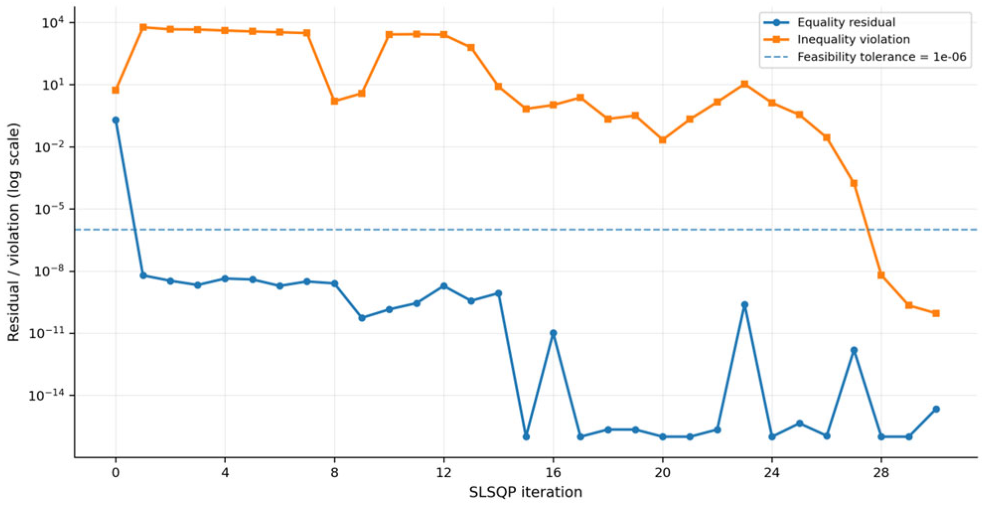
To facilitate its solution, a Python-based computational program is developed to automatically construct the complete constraint set and apply nonlinear optimization using the sequential least squares programming (SLSQP) algorithm implemented in scipy.optimize. Importantly, the proposed approach solves the fuzzy nonlinear constrained optimization problem directly, without transforming it into a fuzzy linear constrained formulation. Although linearization may improve computational efficiency, it can compromise the ability to accurately capture criterion interdependencies, nonlinear fuzzy satisfaction levels, and the behavioral consistency of decision-makers. Details of the computational implementation are presented in a subsequent step.
Step 5. Evaluation of Consistency Ratios (CR) for the FGBWM.
The individual consistency ratios for each D M k , denoted as C R D M k , are computed using Equation (6) [27], while the overall group consistency ratio, C R G e n e r a l , is determined according to Equation (7). In these formulations, ξ D M k   w i t h   k = 1 , . . , K represents the optimal value of ξ D M k   w i t h   k = 1 , . . , K , corresponding to the solution of the FGBWM optimization problem as follows:
C R D M k = ξ D M k / C I ;   k = 1 , , K
C R G e n e r a l = M a x C R D M k = 1 , C R D M k = 2 , . . . , C R D M k = K
Here, CI denotes the corresponding consistency index listed in Table 2 [27].
Step 6. Computer Program for Solving the FGBWM.
As the number of criteria or decision makers increases, constructing the full constraint system for the fuzzy comparison vectors v B x k ~ , v W x k ~ —as illustrated in the first two rows of the constraint system in Equation (5) for D M k   k = 1,…, K-all represented as triangular fuzzy numbers, becomes time-consuming and prone to human error. Conventional fuzzy BWM implementations based on commercial solvers (e.g., LINGO or Excel Solver) typically lack automatic constraint-generation mechanisms, are sensitive to input errors as the number of constraints increases, and exhibit limited computational efficiency when handling large criterion sets or triangular fuzzy inputs. These limitations motivate the development of a dedicated optimization tool capable of automatically generating constraints, managing large-scale fuzzy models, and enabling interactive inspection of results.
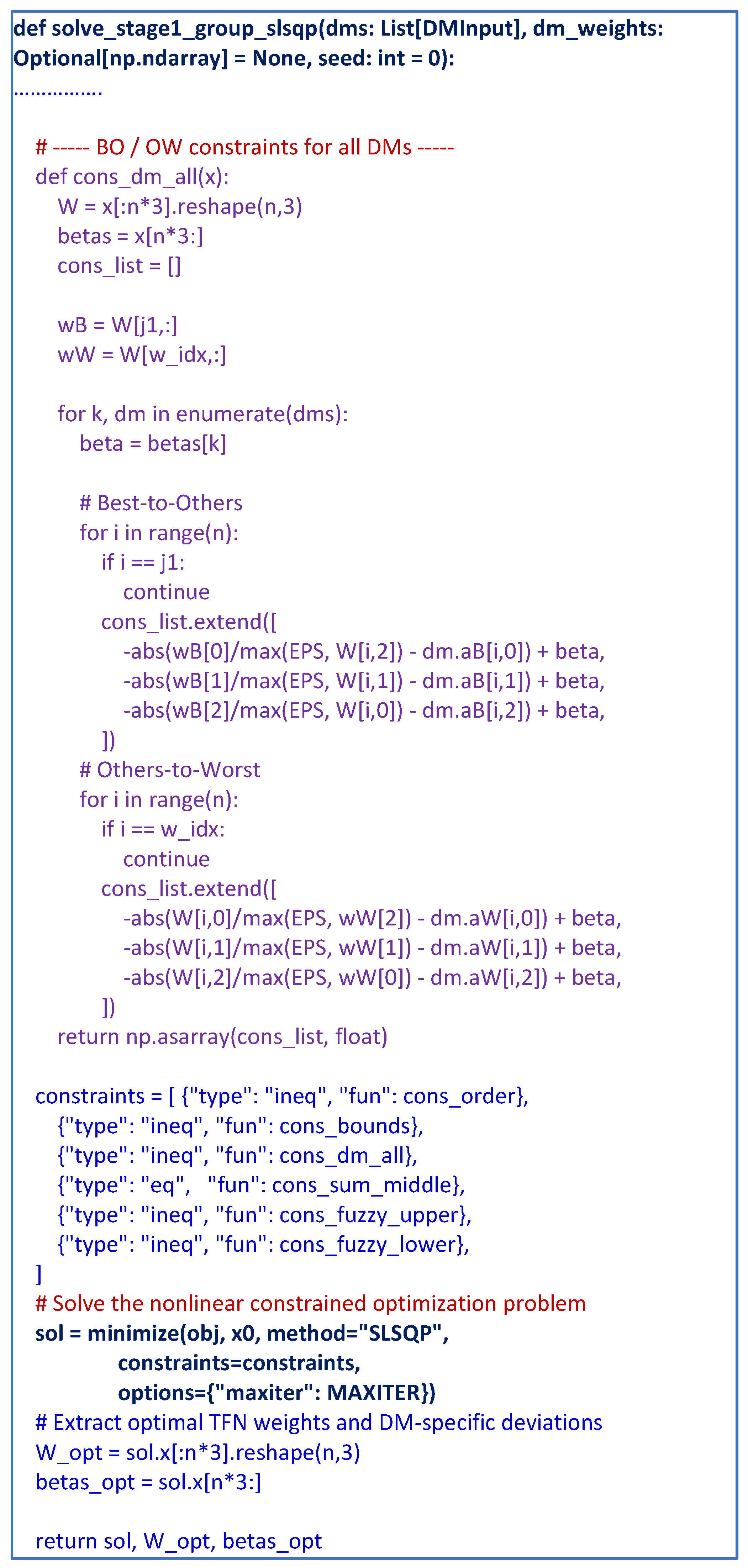
Accordingly, this study develops a Python-based optimization program to solve the proposed FGBWM model (see the flowchart in Figure 1 and a representative code excerpt in Figure 2). The program automatically generates all constraints associated with triangular fuzzy numbers and applies the sequential least squares programming (SLSQP) algorithm implemented in scipy.optimize to efficiently obtain the optimal solution.

3.2.2. Stage 2 of the FIDBWM: Interdependency-Adjusted Criteria Weight Computation

Stage 2 is motivated primarily by the general best–worst method, which incorporates criterion interdependency into the BWM family [37]. Unlike DEMATEL-based models, which mainly aim to reveal causal prominence and net cause–effect structures [42,45,46], the present model uses interdependency information as a BWM-compatible weight-adjustment mechanism.
Stage 2 builds upon the fuzzy group best–worst method by explicitly accounting for interdependencies among criteria under the same multi-expert (multi-DM) setting established in Stage 1. Instead of combining expert inputs at the outset, the interdependency estimation retains DM-specific fuzzy information, thereby preserving uncertainty, expert heterogeneity, and cross-criterion interactions when computing the final weights.
In complex construction decisions—such as selecting a platform/scaffolding system for MEPF works in an airport terminal—criteria rarely behave independently. For example, higher 3D adaptability (Cr5) reduces repositioning and height-adjustment time, which improves deployment efficiency and overall productivity (Cr7). If such relationships are neglected, the resulting weighting structure may deviate from real-world conditions, which can undermine the rationality of the subsequent ranking results.
To address this issue, the model incorporates an expert-elicited fuzzy influence-intensity matrix and propagates these effects to derive interdependency-adjusted weights in an influence-network manner, while maintaining the consistency and computational efficiency of the BWM paradigm. Moreover, preserving DM-level information throughout the process enhances transparency and mitigates information loss in group decision making. Motivated by the interdependency-aware decision analytics framework introduced by Tavana (2023) [37], this study further develops the approach within a triangular fuzzy number (TFN) environment and extends it to a multi–decision-maker context. The proposed formulation preserves decision-maker-specific uncertainty while explicitly modeling cross-criterion influence propagation in a group decision-making setting. The implementation steps of Stage 2 (Steps 7–13) are presented below.
Step 7. Construction of the Fuzzy Influence-Intensity Matrix.
(Modeling pairwise influence intensities among criteria using triangular fuzzy numbers).
To explicitly capture the interdependencies among criteria, this study constructs a fuzzy influence-intensity matrix for each decision maker D M k , k = 1 , 2 , , K . For each decision maker D M k , the fuzzy influence of criterion c r j 1 on criterion c r j j 1 j is expressed as a triangular fuzzy number (TFN) as follows:
I j 1 , j k ~ = l j 1 , j k , m j 1 , j k , u j 1 , j k j 1 , j = 1 , , J ;   j 1 j .
where l j 1 , j k , m j 1 , j k , u j 1 , j k   denote the lower, modal, and upper bounds of the perceived influence intensity, respectively. The TFNs are obtained by transforming experts’ linguistic evaluations of inter-criteria influences into numerical values using the fuzzy linguistic scale presented in Table 4. If no direct causal relationship exists, the corresponding TFN is set to (0,0,0).
All fuzzy influence evaluations provided by DM(k) are assembled into the following fuzzy influence-intensity matrix:
I k = I j 1 , j k ~ J × J , I j , j k ~ = 0 , 0 , 0 .
This matrix-based representation provides a compact, systematic, and computationally efficient framework for modeling interdependencies. Rows represent source criteria, columns denote target criteria. This fuzzy influence matrix captures directionality, intensity, and uncertainty of expert judgments, enabling realistic modeling of complex interdependencies among decision criteria.
Example: To illustrate the fuzzy influence modeling, consider a car-buying problem with five criteria: cr1: quality; cr2: price; cr3: comfort; cr4: safety; and cr5: style. For a given decision maker D M k , the interdependencies among criteria are first elicited using a linguistic influence matrix, where each entry represents the qualitative influence of cri on crj. Diagonal elements are set to NI, indicating no self-influence. Using the linguistic-to-TFN mapping in Table 4, the matrix is converted into a fuzzy influence-intensity matrix I k :
cr1cr2cr3cr4cr5
cr1NIFIWISINI
cr2FINISIVSISI
cr3NIFININIWI
cr4WIVSININIFI
cr5NISIFISINI
cr1cr2cr3cr4cr5
cr1(0,0,0)(1.5,2,2.5)(0.67,1,1.5)(2.5,3,3.5)(0,0,0)
cr2(1.5,2,2.5)(0,0,0)(2.5,3,3.5)(3.5,4,4.5)(2.5,3,3.5)
cr3(0,0,0)(1.5,2,2.5)(0,0,0)(0,0,0)(0.67,1,1.5)
cr4(0.67,1,1.5)(3.5,4,4.5)(0,0,0)(0,0,0)(1.5,2,2.5)
cr5(0,0,0)(2.5,3,3.5)(1.5,2,2.5)(2.5,3,3.5)(0,0,0)
The element I 24 k = 3.5 , 4.0 , 4.5 indicates that price (cr2) exerts a very strong influence (VSI) on safety (cr4), reflecting that higher-priced vehicles typically incorporate more advanced safety technologies. This fuzzy influence matrix compactly captures the direction, strength, and uncertainty of interdependencies and serves as the fundamental input for Stage 2 of the proposed FIDBWM framework.
Step 8. Identification of Influencing Criteria and Reference Criteria (MIC and LIC).
(Determining the most and least influential criteria for each target criterion).
For each criterion c r j and decision maker DM k , the set of influencing criteria is defined as follows:
Ω j k = c r j 1 I j 1 j k ~ 0 , 0 , 0 , j 1 j
Within this set, the most influential criterion (MIC) and the least influential criterion (LIC) with respect to c r j are determined as follows:
c r MIC k , j = arg max c r j 1 Ω j k I j 1 j k ~ = arg max c r j 1 Ω j k m j 1 j k
c r LIC k , j = arg min c r j 1 Ω j k I j 1 j k ~ = arg min c r j 1 Ω j k m j 1 j k
Step 9. Construction of Fuzzy Influence-Intensity Comparison Vectors.
(Deriving most-influential-to-others and others-to-least-influential vectors).
For each D M k   and each criterion c r j , two fuzzy comparison vectors are constructed. Based on the identified MIC and LIC, two influence vectors are constructed for each D M k   and each criterion c r j .
The fuzzy most-to-others influence-intensity vector is defined as v D M k , M j = { v M , j 1 k , j ~ j 1 Ω j k } , and this vector contains Ω j k   elements. Each element is computed as follows:
v M , j 1 k , j ~ = I MIC , j k ~ I i j k ~ , j 1 Ω j k , v M , M k , j ~ = 1 , 1 , 1
where I MIC , j k ~ denotes the fuzzy influence of criterion c r MIC k , j on c r j . For example, considering the column corresponding to c r 2 in the above example, c r 4 is identified as the most influential criterion affecting c r 2 , with an influence intensity represented by the triangular fuzzy number TFN(3.5,4,4.5).
Similarly, the fuzzy others-to-least influence-intensity vector is defined as   v D M k , L j = { v L , j 1 k , j ~ j 1 Ω j k } , and this vector contains Ω j k   elements. Each element is computed as follows:
v L , j 1 k , j ~ = I j 1 j k ~ I LIC , j k ~ , j 1 Ω j k , v L , L k , j ~ = 1 , 1 , 1
where I LIC , j k ~   represents the fuzzy influence of c r LIC k , j on c r j .
Step 10. Multi–Decision-Maker Fuzzy BWM Formulation for Estimating Relative Influence-Intensity Weights.
This study simultaneously incorporates the fuzzy relative influence-intensity comparison vectors estimated by all decision makers into a unified fuzzy nonlinear programming model. For each criterion c r j , the fuzzy BWM model is formulated by considering the fuzzy relative influence-intensity comparison vectors v D M k , M j and   v D M k , L j of all K decision makers.
Let the fuzzy relative influence-intensity weight of criterion c r j 1   on c r j be
w j 1 j ~ = T F N w j 1 j 1 , w j 1 j 2 , w j 1 j 3 , j 1 Ω j k
The multi-decision-maker fuzzy nonlinear optimization problem is defined as
η G e n e r a l j = k = 1 K C o e f _ W D M k η D M k j
Thus, the optimization aims to minimize the deviation in influence-intensity evaluation for each criterion c r j , with each criterion modeled by an individual fuzzy nonlinear optimization problem, as presented below.
min η G e n e r a l j = min k = 1 K C o e f _ W D M k η D M k j
  s . t .   w M I C j ~ w j 1 j ~ v M , j 1 k , j ~ η D M k j w j 1 j ~ w L I G j ~ v L , j 1 k , j ~ η D M k j j 1 Ω j k G r a d M e a n w j 1 j ~ = 1 j C r w j 1 j 2 = 1 w j 1 j 3 + j C r , j j 1 w j 1 j 1 1 w j 1 j 1 + j C r , j j 1 w j 1 j 3 1 w j 1 j ~ = T F N w j 1 j 1 , w j 1 j 2 , w j 1 j 3 ; 0 w j 1 j 1 w j 1 j 2 w j 1 j 3 w h e r e   j 1 = 1 , 2 , , J   a n d   k = 1 , . . , K
Step 11. Construction of the Fuzzy Relative Influence Matrix.
Solving the above optimization model for each criterion c r j yields a fuzzy relative influence–intensity weight vector
w j = w 1 j ~ , , w J j ~ T , j = 1 , , J
where w j 1 j ~ denotes the fuzzy influence intensity of criterion c r j 1 on criterion c r j . For criteria c r j 1 Ω j k , the corresponding influence intensity is set to zero, i.e., w j 1 j ~ = 0 .
The optimal solution η D M k j is subsequently examined using a consistency coefficient analogous to that employed in Stage 1, in order to verify the internal consistency of expert judgments and ensure the reliability of the derived fuzzy influence relationships.
By concatenating these vectors for all j = 1 , , J , the fuzzy relative influence matrix is constructed as
A ~ = w j 1 j ~ J × J , j 1 = 1 , , J A j 1 , j 1 ~ = 1,1 , 1 , A j 1 , j ~ = 0 , 0 , 0   if   no   influnce   exists
In this matrix, rows denote source criteria and columns denote target criteria. The term A ~ j 1 j = w j 1 j ~ represents the fuzzy relative influence intensity of criterion C j 1 on criterion C j . If criterion C j 1 does not influence criterion C j , the corresponding entry is retained as
A j 1 , j ~ = 0 , 0 , 0 .
The diagonal terms are not treated as externally elicited causal influences. Instead, they are introduced as self-retention identities to preserve the baseline contribution of each criterion to itself when interdependency effects are propagated (see [37] for further details):
A j 1 , j 1 ~ = 1 , 1 , 1 , j 1 = 1 , , J .
Step 12. Normalization of the Fuzzy Influence Matrix.
The fuzzy relative influence matrix is normalized column-wise to obtain a redistribution structure for each target criterion. For each column j , the normalization factor is computed from the modal values as follows:
S j = j 1 = 1 J A j 1 j M , S j > 0 .
Using this common positive denominator, each fuzzy element in column j is normalized as follows:
A n o r m ~ = A j 1 , j n o r m ~ J × J
A j 1 , j n o r m ~ = A j 1 j L S j , A j 1 j M S j , A j 1 j U S j
Because the same positive denominator S j is used for the lower, modal, and upper components, the triangular order is preserved: A j 1 j L S j A j 1 j M S j A j 1 j U S j .
Therefore, each normalized value remains a valid TFN. In addition, the modal values in each normalized column sum to one: j 1 = 1 J A j 1 , j n o r m M = 1 .
This confirms that the normalized matrix remains mathematically valid and that each target-criterion column is transformed into a modal-unit fuzzy redistribution structure.
Step 13. Computation of Interdependent Criteria Weights.
Let w ~ i n d = w ~ 1 i n d , w ~ 2 i n d , , w ~ n i n d T denote the independent fuzzy weight vector obtained in Stage 1. The raw interdependency-adjusted fuzzy weights are computed through row-wise matrix–vector propagation, representing an uncertainty-based extension of the crisp-number formulation in [37], as follows:
w ~ j 1 , r a w d e p = j = 1 n A j 1 , j n o r m ~ w ~ j i n d , j 1 = 1 , , J .
Equivalently, in compact matrix form as follows:
w ~ r a w d e p = A n o r m ~ w ~ i n d = w ~ 1 , r a w d e p , . . . , w ~ j , r a w d e p , . . . , w ~ J , r a w d e p T
After this propagation step, the G r a d M e a n sum of the raw propagated TFNs is computed as
S d e p = J = 1 n G r a d M e a n w ~ j , r a w d e p , S d e p > 0 .
The final normalized fuzzy interdependent weights are then obtained before reporting the crisp weights as follows:
w ~ j , n o r m d e p = w ~ j 1 , r a w d e p S d e p = w j 1 , r a w L S d e p , w j 1 , r a w M S d e p , w j 1 , r a w U S d e p .
w ~ n o r m d e p = w ~ 1 , n o r m d e p , . . , w ~ j , n o r m d e p , , w ~ J , n o r m d e p T
Because S d e p is positive, this final fuzzy-level normalization preserves the triangular order of each propagated TFN. To ensure consistency between the fuzzy interdependency propagation and the reported crisp weights, the raw interdependency-adjusted TFNs are normalized using the G r a d M e a n -sum scaling factor before defuzzification. This procedure preserves the triangular order of each TFN and guarantees that the final defuzzified interdependent weights are non-negative and sum to one.
Finally, the crisp interdependent weights are obtained by applying the GMIR operator to the normalized fuzzy interdependent weights as follows:
w j d e p c r i s p = G r a d M e a n w ~ j , n o r m d e p .
Equivalently, this final step can be written as the normalized GMIR form as follows:
w j d e p c r i s p = G r a d M e a n w ~ j , n o r m d e p j = 1 J G r a d M e a n w ~ j , n o r m d e p .
Consequently, the final reported interdependent weight vector satisfies
w j d e p c r i s p 0 , j = 1 J w j d e p c r i s p = 1 .
Therefore, the diagonal terms preserve self-retention, non-active links remain zero, the normalized influence coefficients remain valid TFNs, the propagated interdependency-adjusted TFNs are normalized before G r a d M e a n reporting, and the final crisp interdependent weights are non-negative and sum to one.
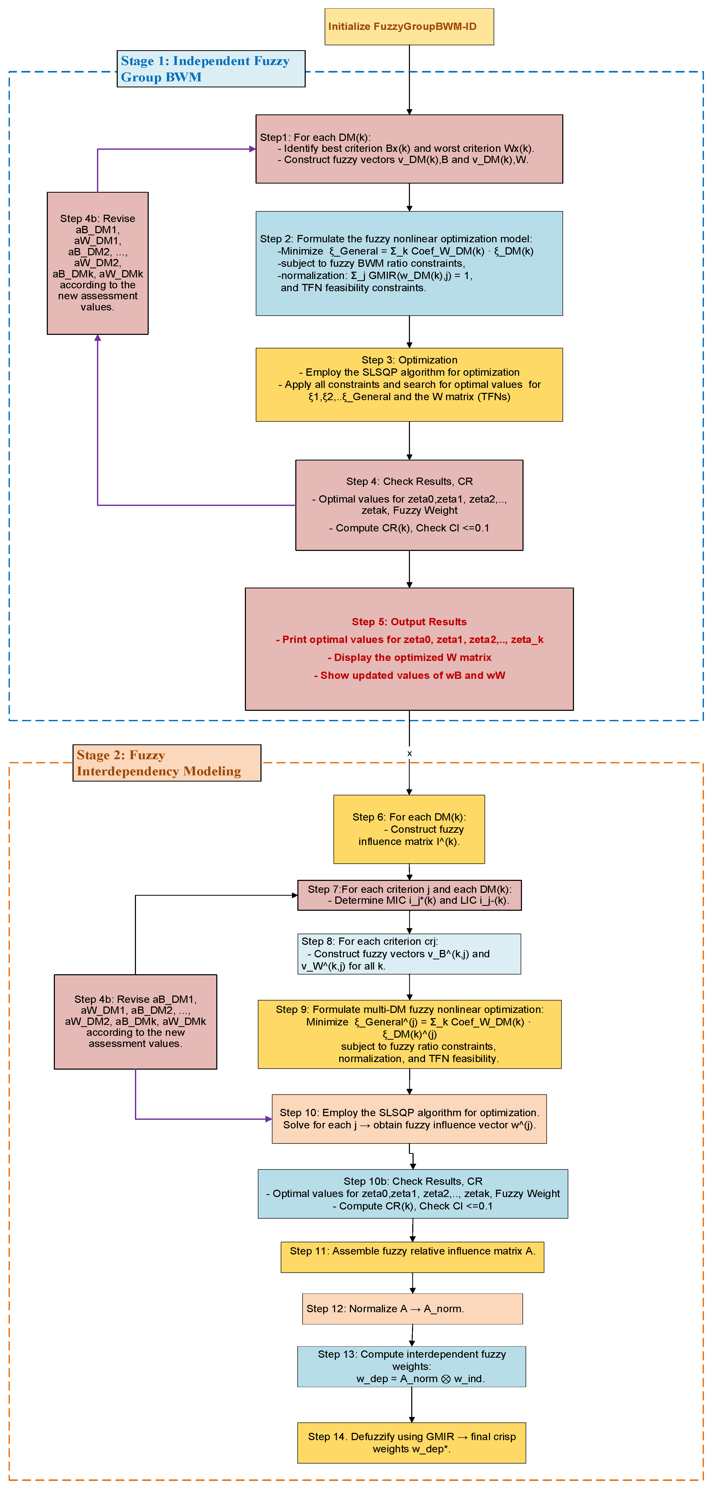
Figure 3 illustrates the flowchart for executing the proposed fuzzy group best–worst model with interdependency (FIDBWM) implemented in Python. The procedure starts by defining the criteria set Cr and the group of decision-makers D M k . Fuzzy BWM judgments for the best and worst criteria ( v B x k ~ ,   v W x k ~   ,   k = 1 , . . , K ) are then elicited from each decision maker D M k . In Stage 1, a fuzzy group BWM optimization is performed to derive the independent fuzzy weights w ~ i n d . In Stage 2, fuzzy influence matrices I k are constructed to identify the most influential criteria (MIC) and least influential criteria (LIC) for each criterion and decision-maker. Based on these matrices, a multi-decision-maker fuzzy interdependency optimization is carried out to obtain the normalized relative influence matrix A n o r m and compute the interdependent fuzzy weights w ~ n o r m d e p . All computational procedures were implemented in Python and executed in a local CPU-based computing environment. The proposed FIDBWM was developed using the SLSQP optimization algorithm in Python, without reliance on commercial optimization solvers.

3.3. Fuzzy TOPSIS for Assessing the Performance of Alternatives

After deriving the criterion weights using the proposed FIDBWM with multiple decision-makers, fuzzy TOPSIS is applied to evaluate and rank access platform system alternatives for MEP installation in the airport terminal project. TOPSIS [54] is widely recognized as a robust multiple criteria decision-making (MCDM) method and has been extensively used in contractor selection studies.
The method is based on selecting the alternative that is closest to the positive ideal solution (PIS), which minimizes cost criteria and maximizes benefit criteria, and farthest from the negative ideal solution (NIS). This study adopts the distance measure between two triangular fuzzy numbers x ~ 1 = a 1 , b 1 , c 1 , x ~ 2 = a 2 , b 2 , c 2   proposed by Chen et al. (2000) [47], as defined in Equation (23).
d x ~ 1 , x ~ 2 = 1 3 a 1 a 2 2 + b 1 b 2 2 + c 1 c 2 2
This study adopts the fuzzy TOPSIS procedure described in [48,49], which employs triangular fuzzy numbers (TFNs) to handle imprecise numerical information. The methodology is implemented through the following steps:
Step 1. Assign fuzzy ratings to the alternatives under each criterion.
Using the evaluations provided by the decision-makers, the fuzzy decision matrix D ~ is constructed as follows, together with the fuzzy weight vector w j ~ =   T F N w j 1 , w j 2 , w j 3 . Each element x ~ i j = a i j , b i j , c i j denotes the fuzzy performance rating of alternative A i with respect to criterion Cj. Here, I and J indicate the numbers of alternatives and evaluation criteria, respectively.
C 1 C 2 C j C J D ~ = A 1 A 2 A I x ~ 1 , 1 x ~ 1 , 2 x ~ 1 , J x ~ 2 , 1 x ~ 2 , 2 x ~ 2 , J x ~ I , 1 x ~ I , 2 x ~ I , J , w ~ = w ~ 1 w ~ 2 w ~ J ,
For cases involving K decision-makers, the aggregated fuzzy rating x ~ i j is obtained by taking the minimum of a i j k , the average of b i j k , and the maximum of c i j k .
Step 2. Compute the normalized fuzzy decision matrix.
The normalized fuzzy decision matrix is expressed as R ~ = r i j ~ , where r i j ~ is computed using Equations (24) and (25) for benefit and cost criteria, respectively. Here, c j and a j denote the maximum and minimum reference values across alternatives. A max–min normalization scheme following Nadaban Sorin et al. (2016) [48] is adopted.
r ~ i j = a i j c j , b i j c j , c i j c j , j B ;   ( B e n e f i t   c r i t e r i a )
r ~ i j = a j c i j , a j b i j , a j a i j , j C ;   C o s t   c r i t e r i a
Here, c j = m a x i   ( c i j )   if   j B ; and a j = m i n i   ( a i j )   if   j C .
Step 3. Compute the weighted normalized fuzzy decision matrix.
The weighted normalized fuzzy decision matrix is determined by Equation (26), as follows:
V ~ = v ~ i j I × J = v i j 1 , v i j 2 , v i j 3 I × J   f o r   i = 1 , 2 , , I ;   j = 1 , 2 , , J
where v ˜ i j = r ˜ i j w ˜ j = v i j 1 , v i j 2 , v i j 3 .
Step 4. Determine FPIS and FNIS.
The fuzzy positive ideal solution (FPIS) and fuzzy negative ideal solution (FNIS) are defined as
A = v ˜ 1 , v ˜ 2 , , v ˜ J
where v ˜ j =   m a x i   ( v i j 3 )   and v ˜ j = m i n i   ( v i j 1 ) ,   j = 1 ,   2 , ,   J ; i = 1 ,   2 , ,   I .
Step 5. Calculate distance to FPIS and FNIS.
For each alternative A i , distances to FPIS and FNIS are computed as d i and d i as follows:
d i = j = 1 J     d v ˜ i j , v ˜ j ,   i = 1 , 2 , ,   I
Step 6. Compute the closeness coefficient.
The closeness coefficient of alternative Ai is calculated as
C C i = d i d i + d i , i = 1 , 2 , , I
Step 7. Rank the alternatives.
Alternatives are ranked in descending order of C C i , and the alternative with the highest value is selected as the preferred option.

3.4. Fuzzy VIKOR

VIKOR is a compromise-based multi-criteria decision-making (MCDM) method developed for optimizing complex systems under conflicting criteria. Given the criteria weights w j (for criteria C j , j = 1 , , J ) and the performance ratings of each alternative A i (i = 1 , , I ), the method produces (i) a compromise ranking and (ii) a recommended compromise solution that balances overall group utility and the maximum individual regret [50].
The original VIKOR formulation is based on the L p , i metric, which measures the normalized distance of alternative A i from the ideal performance across all criteria [50] as follows:
L p , i = j = 1 J f j f i j f j f j p 1 / p , 1 p , i = 1 , 2 , , I .
where f j and f j denote the best and worst values for criterion j , and f i j is the (defuzzified) performance of alternative i on criterion j . In practice, VIKOR mainly uses L 1 , i and L , i to define the two ranking measures S i (group utility) and R i (regret).
The step-by-step algorithm of the simplified fuzzy VIKOR method is presented below, in accordance with [51,52].
Step 1. Define the decision setting. Specify the alternatives A i (e.g., platform options) and the evaluation criteria C j , including the criterion type (benefit or cost).
Step 2. Collect fuzzy assessments and fuzzy weights. For each decision maker k = 1 , , K , triangular fuzzy ratings are elicited x i j k ~ = a i j k , b i j k , c i j k and obtain fuzzy criterion weights w j ~ =   T F N w j 1 , w j 2 , w j 3 from the fuzzy BWM stage.
Step 3. Aggregate the fuzzy ratings across decision makers. Compute the aggregated triangular fuzzy rating for each i , j using the min–mean–max rule as follows:
a i j = min k a i j k , b i j = 1 K k = 1 K b i j k , c i j = max k c i j k
Using the aggregated values, form the fuzzy decision matrix D ~ = x i j ~ I × J .
Step 4. Defuzzify the fuzzy decision matrix (and weights). Convert each triangular fuzzy rating to a crisp value using the Center of Area (COA) method. The same defuzzification can be applied to w j ~ to obtain crisp weights w j when required.
x i j = a i j + c i j a i j + b i j a i j 3
Step 5. Identify the best and worst values for each criterion.
The best value f j and the worst value f j of all criterion ratings are calculated as follows:
f j = m a x i x i j , and   f j = m i n i x i j
Step 6. Compute S i (group utility) and R i (maximum regret). Using the crisp weights w j , calculate the weighted normalized distances to the ideal for each alternative as follows:
S i = j = 1 J w j f j x i j f j f j , i = 1 , 2 , , I .
R i = max j w j f j x i j f j f j , i = 1 , 2 , , I .
Here, S i reflects the overall closeness to the ideal solution (higher group utility), while R i captures the worst-case deviation on any single criterion (regret). Typically, S i and R i lie in 0 , 1 , and smaller values indicate better performance.
Step 7. Compute the compromise index Q i and rank the alternatives. Let S = min i S i , S = max i S i , R = min i R i , and R = max i R i . Then compute
Q i = ν S i S S S + 1 ν R i R R R , i = 1 , 2 , , I .
where ν 0 ,   1 controls the trade-off between the majority strategy (group utility) and the opponent strategy (regret). A common default is ν = 0.5 . Rank alternatives in ascending order of Q i .
Compromise solution conditions.
Let A 1 and A 2 denote the first and second alternatives in the ascending Q ranking. The top-ranked alternative A 1 is accepted as the compromise solution if both conditions hold:
  • Cond. 1 (acceptable advantage):  Q A 2 Q A 1 1 / I 1   (39).
  • Cond. 2 (stability):  A 1 is also ranked best by S i and R i .
If either condition is not satisfied, VIKOR recommends a set of compromise solutions (e.g., the top few alternatives) for further engineering judgment.

3.5. Validation of the Proposed MCDM Framework

(a) 
Comparative analysis of the proposed FIDBWM model.
To demonstrate the validity and effectiveness of the proposed approach, comparative analyses are conducted between the proposed FIDBWM model, which explicitly incorporates multiple decision-makers and accounts for interdependencies among criteria, and existing BWM-based models reported in the literature, including those proposed by Safarzadeh et al. (2018) [25] and Tavana et al. (2023) [37]. Specifically, the model of Safarzadeh et al. [25] considers a group decision-making context but is formulated in a crisp environment and does not address interdependencies among criteria. In contrast, the approach of Tavana et al. [37] captures interrelationships among criteria; however, it is developed under a crisp setting and does not explicitly model multiple decision-makers simultaneously within the decision-making framework. The comparative results are summarized in Appendix A, which presents a detailed comparison between the proposed FIDBWM model with multiple decision-makers and the alternative models.
(b) 
Validation of the proposed hybrid MCDM model.
Validation of multi-criteria decision-making (MCDM) models requires methodological rigor, internal consistency, and acceptance by both domain experts and relevant stakeholders. A fundamental validation strategy involves benchmarking the model outcomes against established or alternative approaches to assess robustness and reliability. In addition, expert judgment is employed to evaluate the logical coherence and practical credibility of the results based on domain-specific knowledge. Comparative assessment using multiple MCDM techniques further strengthens the validation process by revealing relative advantages, limitations, and result stability. Accordingly, this study employs fuzzy TOPSIS and fuzzy VIKOR as benchmarking methods, complemented by expert-based validation, to confirm the reliability and practical applicability of the proposed hybrid MCDM framework.

3.6. Integrated FGBWM–TOPSIS and Robustness Assessment Methodology with Computational Pseudocode

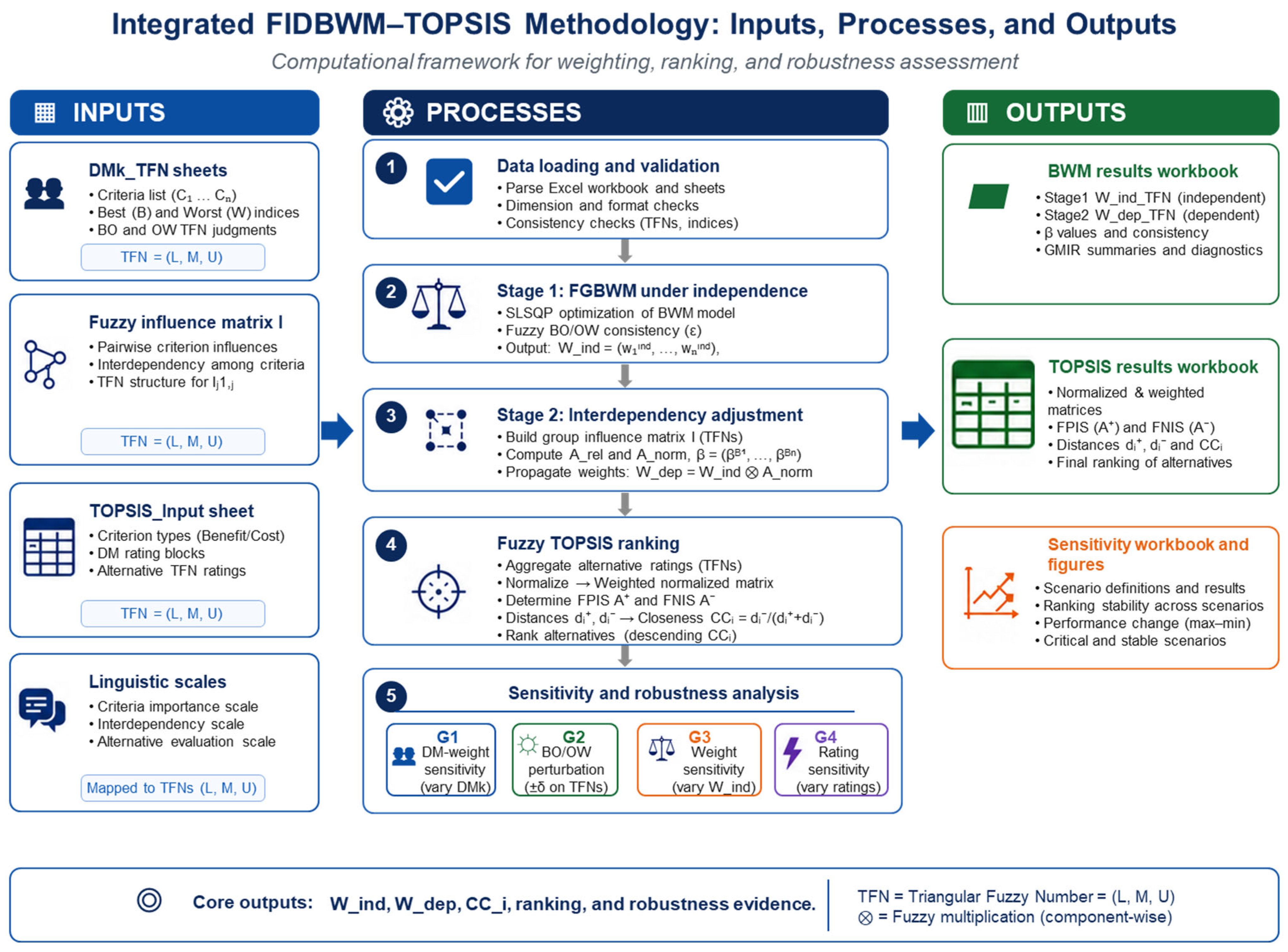
To improve the transparency, traceability, and methodological clarity of the proposed framework, Figure 3 presents the integrated FIDBWM–TOPSIS computational workflow, which links the Excel-based input structures, the two-stage FIDBWM weighting procedure, the fuzzy TOPSIS ranking process, and the sensitivity-analysis outputs within a single end-to-end implementation.
In addition, Table 5 provides the corresponding integrated pseudocode of the FIDBWM–TOPSIS workflow, including the main input templates, Stage 1 and Stage 2 SLSQP-based weighting procedures, fuzzy TOPSIS ranking steps, SLSQP multi-start robustness assessment, and four-group sensitivity analysis. Together, Figure 3 and Table 5 clarify how the proposed framework is computationally implemented from expert-input preparation to final ranking and robustness diagnostics.

3.7. Comparison and Novelty of the Proposed FIDBWM Method

The proposed FIDBWM–TOPSIS framework should be understood as a methodological extension and operational integration of the BWM family rather than as an unrelated new MCDM method. Its novelty lies in the formal way uncertainty, group decision making, and criterion interdependency are jointly embedded within a BWM-compatible fuzzy nonlinear optimization structure and then connected to fuzzy TOPSIS for alternative ranking.
To address the need for a more formal comparison, Table 6 summarizes the main mathematical differences between the proposed FIDBWM framework and related BWM-, GBWM-, and DEMATEL-based approaches. The comparison emphasizes not only whether uncertainty or interdependency is considered, but also how these elements are mathematically introduced into the weighting engine.
Table 6 clarifies that the proposed method is not novel merely because it combines BWM and TOPSIS. The substantive mathematical extension is located in the weighting engine. In Stage 1, the model derives independent fuzzy weights by minimizing a weighted group consistency deviation while retaining decision-maker-specific deviations and fuzzy BO/OW judgments. In Stage 2, the model converts expert-elicited fuzzy influence information into BWM-style relative influence-intensity comparison vectors for each target criterion. These vectors are solved through fuzzy nonlinear optimization and assembled into the relative influence matrix and the normalized influence matrix. The normalized matrix is then used to propagate W_ind into W_dep.
This design differs from DEMATEL-based dependency modeling. DEMATEL primarily aims to reveal causal structures through direct- and total-relation matrices. By contrast, the proposed FIDBWM framework treats interdependency as a BWM-compatible weight-adjustment mechanism. The goal is not to produce a cause–effect map, but to obtain independent and interdependency-adjusted fuzzy weights that can be directly used in fuzzy TOPSIS ranking.
The proposed method also extends the logic of GBWM. GBWM provides a basis for incorporating interdependency within the BWM family; however, the present framework adds triangular fuzzy uncertainty, embedded multi-decision-maker modeling, decision-maker-specific deviation handling, automated nonlinear constraint generation, and a construction-oriented fuzzy TOPSIS ranking workflow. Therefore, the proposed contribution is best described as a fuzzy group interdependency-aware BWM weighting engine integrated with fuzzy TOPSIS, rather than a purely descriptive hybridization of existing methods.
In summary, the main mathematical novelty of the proposed FIDBWM method consists of four connected components: (i) a multi-DM fuzzy scalar deviation-minimization objective; (ii) TFN-based BO/OW and influence-intensity consistency constraints; (iii) fuzzy relative influence-intensity modeling and normalized propagation from W_ind to W_dep; and (iv) direct coupling of W_dep with fuzzy TOPSIS and robustness diagnostics in an automated computational workflow.

4. Application of the Proposed FIDBWM–TOPSIS Framework

This section presents the application of the proposed multi-criteria decision-making (MCDM) framework to the selection of MEP access platform systems in complex airport terminal projects.

4.1. Project Description

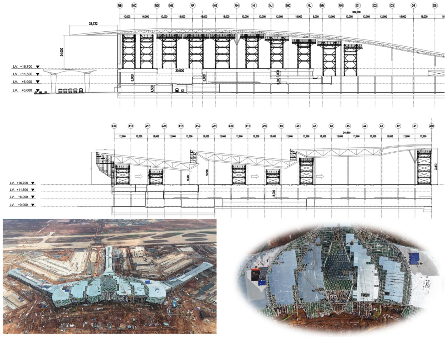
The International Airport Project located in Ho Chi Minh City, Viet Nam (see Figure 4), is being developed as a large-scale aviation facility and a strategic hub within the regional air transport network. Upon full completion, the airport is expected to accommodate approximately 100 million passengers annually. This case study focuses on Phase I of the project, which is designed for a capacity of 25 million passengers per year and is regarded as the most technically demanding construction stage.
Phase I comprises a passenger terminal with a total gross floor area of approximately 373,000 m2, with ceiling elevations on the upper levels ranging from +16.7 m to +40.7 m. The significant vertical variation, combined with the architectural complexity of the terminal, imposes stringent requirements on the installation of Mechanical, Electrical, Plumbing, and Firefighting (MEPF) systems. These challenges are further intensified by the current conditions of the construction labor market in Viet Nam, characterized by shortages of skilled workers, heightened safety concerns, and increasing productivity pressures, particularly for high-elevation and large-span construction activities. In parallel, the domestic scaffolding and access platform industry is transitioning from conventional labor-intensive systems toward mechanized and modular solutions; however, the level of automation and professional deployment remains limited, largely due to the need for specialized training that is not yet uniformly available across the workforce.
This airport terminal project provides a highly suitable and practically significant case study for the proposed FIDBWM–TOPSIS framework because the access platform selection problem in this complex project is inherently multi-criteria, uncertain, and affected by strong interdependencies among evaluation criteria.
In Phase I of the project, MEP installation must be executed under complex geometric conditions, large ceiling height variations, limited workspace, and strict safety and schedule requirements. Under such conditions, platform alternatives cannot be evaluated using a single performance measure, since technical compatibility, structural stability, worker safety, deployment efficiency, cost efficiency, and sustainability must all be considered simultaneously. Moreover, these criteria do not act independently. For example, better 3D adaptability can improve deployment efficiency and productivity, while higher load capacity and stability can directly affect both safety and operational performance. Therefore, this project represents a realistic decision environment in which uncertainty, expert judgment, and criterion interdependencies play a decisive role. For this reason, the case offers a strong and credible basis for demonstrating the applicability and practical value of the proposed framework.

4.2. Application of the Proposed FIDBWM and TOPSIS Model to the Case Study

4.2.1. Identification of Evaluation Criteria for the Case Study

The contractor’s expert group, representing the main contractor responsible for the execution of scaffolding and access platform systems for MEP construction works, comprises two senior specialists, whose key profiles are summarized in Table 7. In this case study, the Expert Evaluation Group serves as the decision-making body, tasked with determining the relative importance (weights) of the evaluation criteria and assessing the performance of alternative scaffolding and access platform systems supporting MEP installation at different elevations.
Expert Selection Criteria and Functional Diversity
The two decision makers were selected based on project-specific expertise and functional relevance rather than statistical sampling criteria. Both experts have more than 20 years of professional experience, hold senior decision-making positions, and have direct involvement in complex construction projects involving temporary works, high-elevation access systems, and MEPF coordination. Expert 1 contributes a construction execution and temporary-works perspective, with particular emphasis on structural safety, construction methods, erection feasibility, and high-elevation platform deployment. Expert 2 contributes an MEP coordination and site-logistics perspective, with particular emphasis on trade interference, workface continuity, sequencing constraints, and operational feasibility.
Accordingly, the expert panel represents two complementary functional perspectives within the contractor’s project team. This selection is consistent with the practical decision context of the case study, because the selection of access-platform systems primarily falls within the responsibility and authority of the construction contractor. In construction practice, the contractor is directly responsible for selecting and managing construction means and methods, including temporary works, access systems, equipment deployment, workface organization, and safety-related execution measures. By contrast, the client typically focuses on controlling final deliverables, performance requirements, quality outcomes, and contractual compliance rather than prescribing the contractor’s detailed construction means and methods.
Therefore, the case study should be interpreted as a project-specific decision-support demonstration rather than a statistically generalizable survey. To further reduce the risk that the final recommendation is driven by a single fixed expert-input configuration, an expert-input and ranking robustness analysis has been added in the results Section 4.4. This additional analysis examines whether the preferred alternative remains stable under variations in expert-related inputs, thereby strengthening the credibility and practical reliability of the proposed decision-support framework.
Drawing on a comprehensive review of factors affecting the effectiveness of temporary works and construction support systems reported in the literature, together with practical experience from comparable large-scale construction projects involving scaffolding systems in Viet Nam, the expert group collectively identified and reached consensus on a set of nine evaluation criteria. These criteria represent critical technical, operational, safety, and constructability considerations relevant to MEP construction activities and are used to evaluate and compare alternative access platform solutions within the proposed decision-making framework. The finalized criteria set is presented in Table 8.

4.2.2. Stage 1: Criteria Weighting Under the Independence Assumption

In Stage 1, criteria weights are derived under the assumption that all criteria are mutually independent. Linguistic judgments are elicited from two decision makers (DM1 and DM2) for the LTIA MEPF platform-system selection problem.
Both experts identify the same best (Cr1) and worst criterion (Cr9). Nevertheless, DM2’s evaluations are not identical to those of DM1; selected criteria are intentionally rated at relatively higher or lower importance levels to reflect heterogeneous expert perspectives while preserving structural consistency.
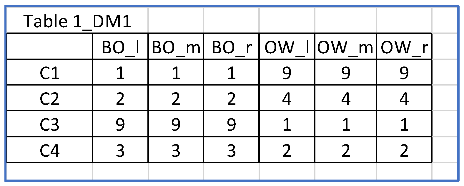
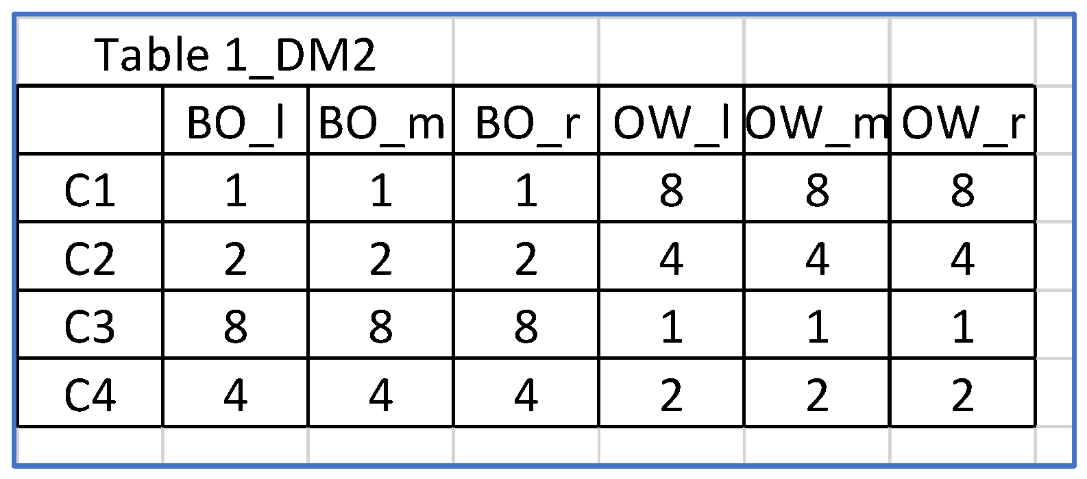
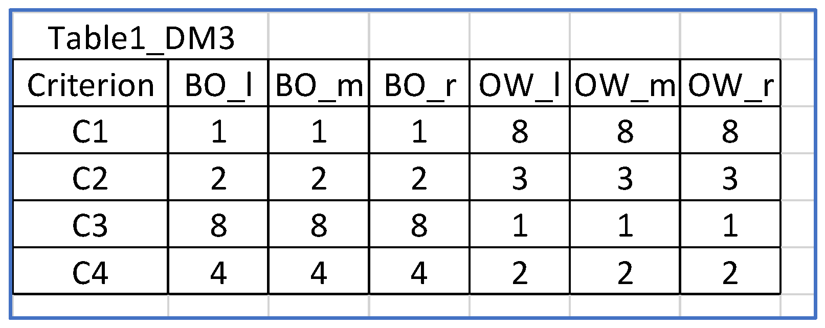
Based on these judgments, the best-to-others (BO) and others-to-worst (OW) linguistic comparison vectors are constructed for each decision maker using the fuzzy BWM scale. The resulting BO/OW vectors, presented in the following tables (Table 9 and Table 10), serve as direct inputs to the proposed FIDBWM model in Stage 1.
Furthermore, a consensus was reached among the experts to assign equal weighting coefficients ( C o e f W D M 1 = C o e f W D M 2 = 0.5 ). Accordingly, the optimization model for the case study is formulated as follows:
m i n ξ G e n e r a l = 0.5 ξ D M 1 + 0.5 ξ D M 2
s . t .   w B x 1 w j 3 v B x , j k = 1 1 ξ D M 1 ; w B x 2 w j 2 v B x , j k = 1 2 ξ D M 1 ; a n d w B x 3 w j 1 v B x , j k = 1 3 ξ D M 1 ; j = 1 , 2 , , 9 w B x 1 w j 3 v B x , j k = 2 1 ξ D M 2 ; w B x 2 w j 2 v B x , j k = 2 2 ξ D M 2 ; a n d w B x 3 w j 1 v B x , j k = 2 3 ξ D M 2 ; j = 1 , 2 , , 9 j = 1 9   G r a d M e a n w j ~ = j = 1 J   1 6 w j 1 + 4 w j 2 + w j 3 = 1 j C r w j 2 = 1 w j 1 3 + j C r , j j 1 w j 1 1 w j 1 1 + j C r , j j 1 w j 3 1 w j ~ = T F N w j 1 , w j 2 , w j 3 ; w j 1 w j 2 w j 3 ; w j 1 0 w h e r e   j = 1 , 2 , , 9   a n d   k = 1 , 2
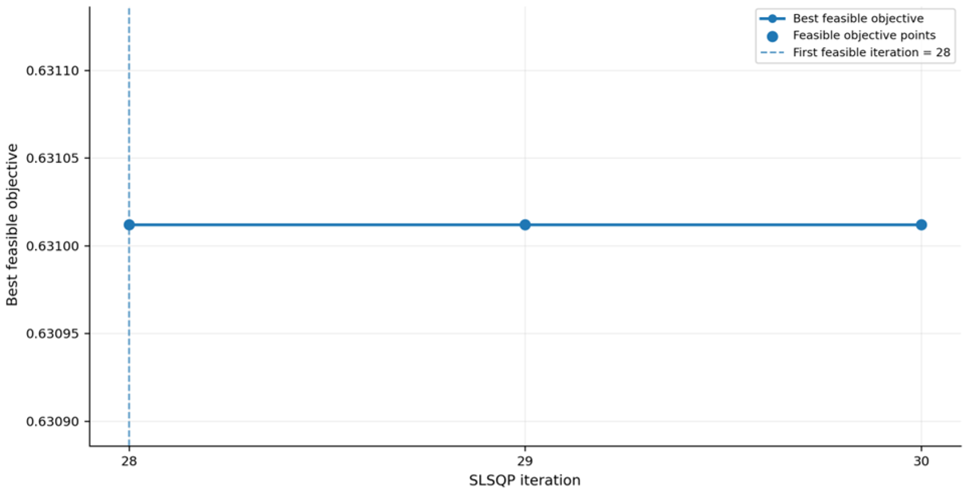
To solve the nonlinear optimization problem defined in Equations (38) and (39), a Python-based program following the algorithmic procedure illustrated in Figure 3 was employed. The optimal objective values obtained are ξ D M 1 =   0.631   and ξ D M 2 = 0.631 . As reported in Table 11 and Table 12, the consistency index (CI) is 9.35. Using Equations (7) and (8), the consistency ratios are calculated as C R D M 1 = 0.631 / 9.35 = 0.067 and C R D M 2 = 0.631 / 9.35 = 0.067 . The overall consistency ratio, defined as C R G e n e r a l = max C R D M 1 , C R D M 2 , equals 0.067 , which is well below the acceptable threshold of 0.1, indicating a high level of consistency in the decision-making process.

4.2.3. Stage 2: Criteria Weighting Under Interdependencies

For the MEPF platform system selection case study of the airport project, linguistic evaluations from two decision makers (DM1 and DM2) are employed to elicit interdependencies among criteria. In the first step, the experts jointly discuss and agree on the existence or absence of interdependency relationships between criterion pairs, thereby establishing a common interdependency structure. In addition, for each target criterion c r j , the two experts agree on the most influential and least influential criteria within the interdependency framework to ensure structural comparability.
Given this shared structure, each decision maker individually evaluates the influence intensity of interacting criteria relative to the predefined best and worst reference criteria using a fuzzy linguistic scale. Although the influence ratings provided by DM2 may differ from those of DM1, the interdependency structure and the reference criteria remain fixed. Accordingly, fuzzy interdependency matrices are constructed for each decision maker. Table 13 and Table 14 present the fuzzy interdependency matrices evaluated by DM1, while Table 15 and Table 16 report those evaluated by DM2. These matrices are then directly used as inputs to the proposed FIDBWM model in Stage 2.
Next, by implementing Steps 7–12, Table 17 presents the normalized fuzzy influence matrix, as shown below:
Accordingly, by applying Equation (19), the corresponding optimal dependent criteria weights are provided in Table 18, while the objective function values η D M k j are summarized in Table 19. All consistency ratio values satisfy the required threshold conditions.
The criteria weights obtained after accounting for interdependencies are subsequently used to evaluate the alternative scaffolding/platform systems for MEP construction in the airport project using the fuzzy TOPSIS method.
Discussion of Independent and Interdependent Criteria Weights
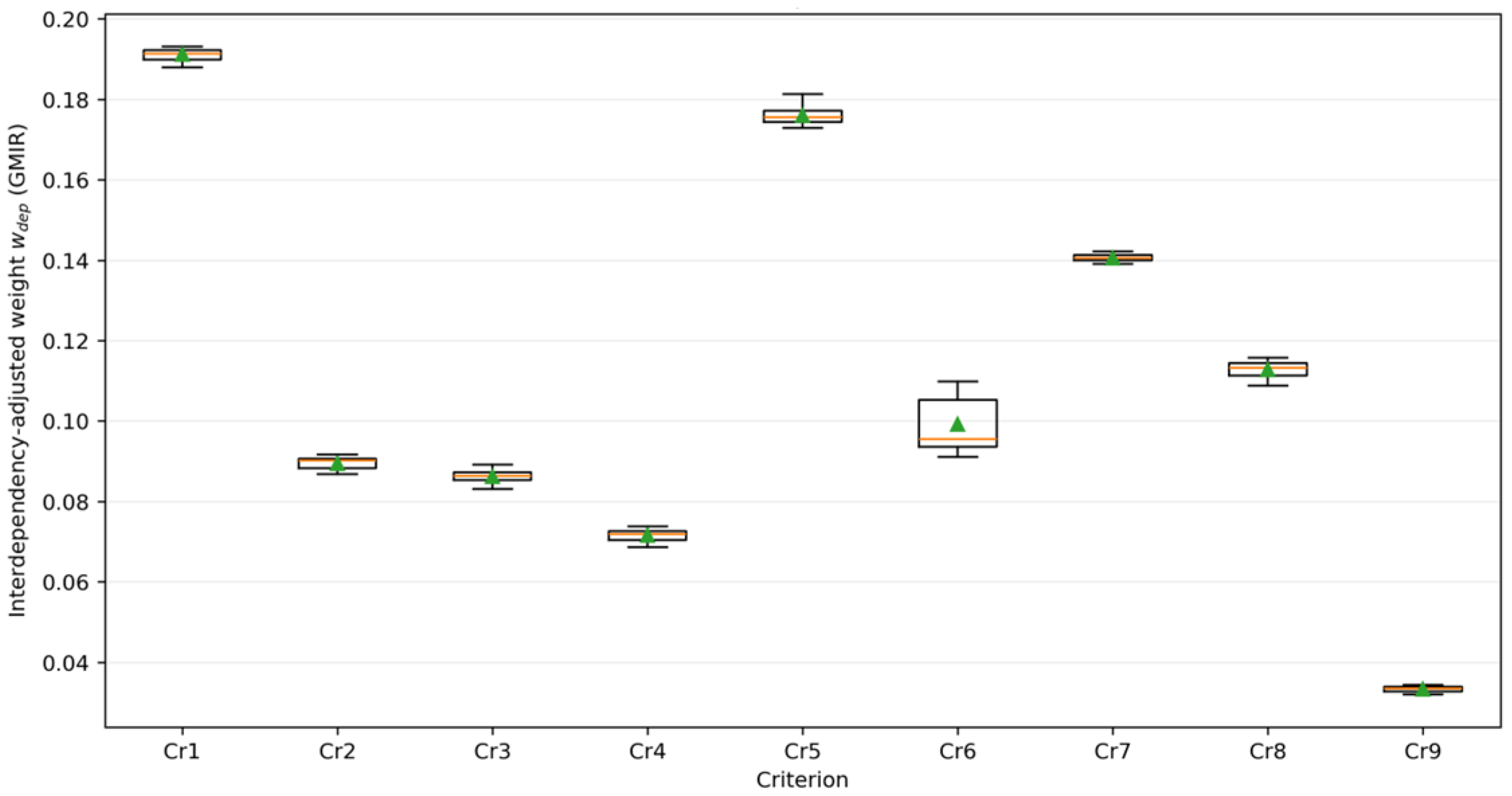
The comparison between independent and interdependent criteria weights reveals a clear redistribution of importance once interdependencies are incorporated. Several criteria experience noticeable shifts, indicating that ignoring inter-criteria interactions may lead to biased importance estimation.
In particular, w 1 ~ shows a substantial decrease (Delta = −0.034), suggesting that although it is dominant under the independence assumption, its relative importance is moderated when mutual influences with other criteria are considered. Conversely, w 3 ~ and w 5 ~ exhibit pronounced increases (Delta = 0.025 and 0.039, respectively), reflecting their strong roles as influenced and influencing criteria within the interdependency network.
These changes are consistent with the elicited linguistic interdependency matrices from both decision makers, where criteria associated with high mutual influence intensities (VSI/SI) tend to gain importance in the dependent weighting scheme. Overall, the results confirm that the proposed FIDBWM framework effectively captures hidden interaction effects among criteria, leading to more realistic and structurally informed weighting outcomes for subsequent decision analysis.

4.2.4. Evaluation of Access Platform System Alternatives

Performance Evaluation Using the Fuzzy TOPSIS Method
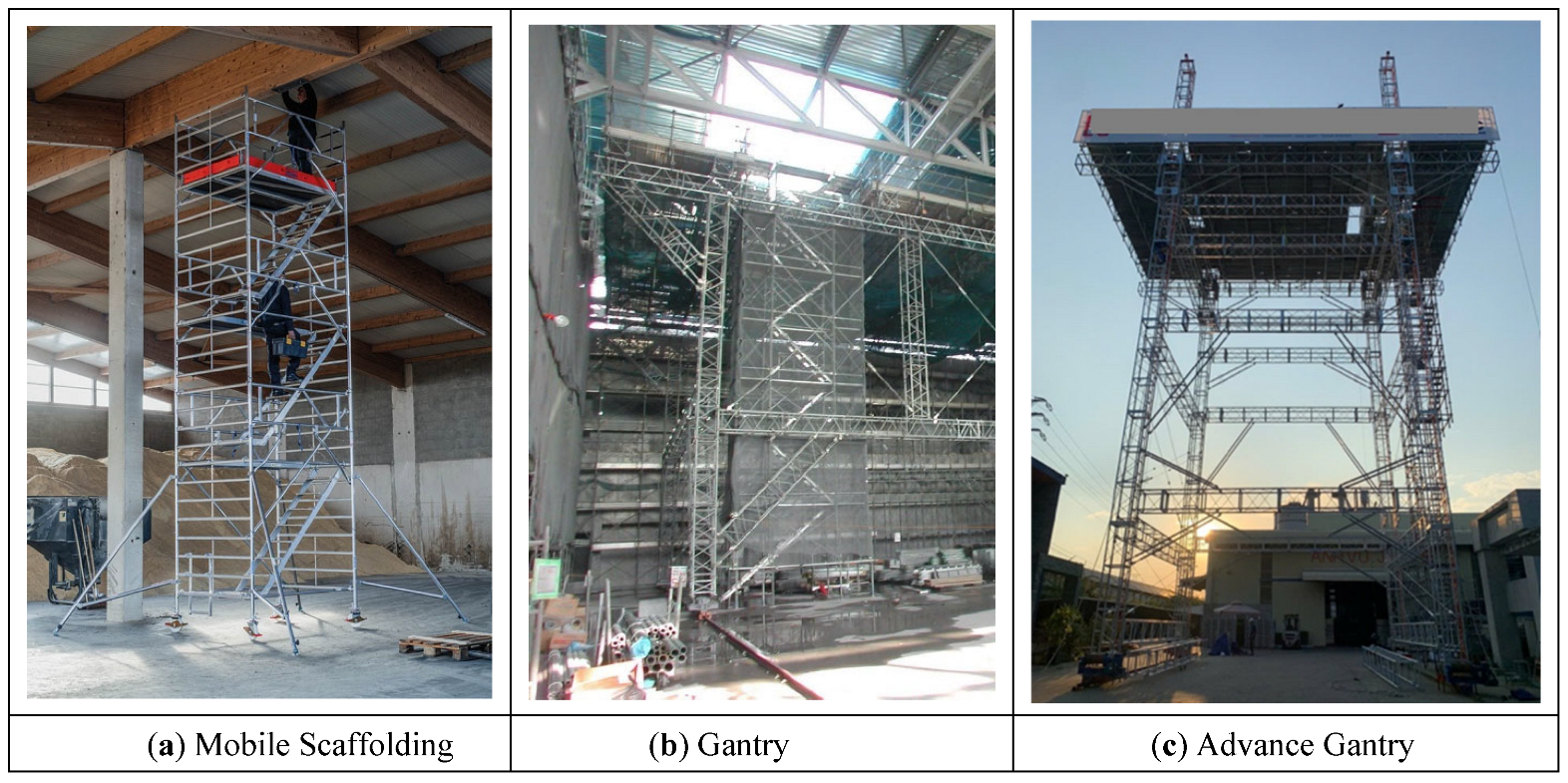
Based on preliminary design information, site conditions, construction planning constraints, and safety requirements for suspended MEP installation, the contractor’s expert team identified three feasible access platform system alternatives for evaluation. These alternatives were formulated to support MEP works in large-span spaces and at significant ceiling elevations, while satisfying requirements related to structural stability, operational efficiency, and occupational safety. The configurations of the three alternatives are illustrated in Figure 5.
Figure 5 depicts the considered the following access platform systems: (a) mobile scaffolding, (b) a gantry-based platform system, and (c) an advanced gantry system. The alternatives differ in terms of structural capacity, mobility, and operational flexibility, representing commonly adopted solutions in contemporary large-scale construction projects.
  • Alternative 1 (Alt. 1—Mobile Scaffolding): As shown in Figure 5a, mobile scaffolding is a lightweight and modular access system intended primarily for personnel access. Its portability allows flexible deployment in confined or indoor environments, making it suitable for light MEP installation and maintenance tasks.
  • Alternative 2 (Alt. 2—Gantry-Based Platform System): Figure 5b presents a gantry-type platform characterized by a robust structural configuration and horizontal mobility along fixed rails. The system is capable of supporting heavy equipment and materials and enables efficient coverage of large working areas.
  • Alternative 3 (Alt. 3—Advanced Gantry System): As illustrated in Figure 5c, the advanced gantry system integrates horizontal rail movement with vertical adjustability of the working platform. This configuration provides high load-bearing capacity and enhanced adaptability, allowing rapid adjustments in both elevation and position under complex site conditions.
The relative performance of the three alternatives was quantitatively evaluated using the fuzzy TOPSIS method based on nine predefined criteria. Two experts independently assessed the alternatives using a nine-level linguistic scale (Table 3), and the corresponding fuzzy evaluations are reported in Table 20, Table 21, Table 22 and Table 23. Based on these results, Table 24 presents the consolidated triangular fuzzy evaluation of the three alternatives aggregated from the two decision-makers.
The evaluation results derived from the linguistic scale in Table 20 are converted into triangular fuzzy numbers (TFNs), as illustrated in Table 21.
Next, the steps for calculating the weighted normalized fuzzy decision matrix are presented in Table 25. Following this, the process involves computing the distance of each alternative from the fuzzy positive ideal solution (FPIS) as shown in Table 26, and from the fuzzy negative ideal solution (FNIS) as shown in Table 27. Finally, the closeness coefficient ( C C i ) for each alternative is computed, as shown in Table 28.
Using criterion weights derived from the multi-expert FIDBWM model, fuzzy TOPSIS was applied to evaluate three access-platform alternatives: Alt 1, mobile scaffolding; Alt 2, gantry systems; and Alt 3, advanced gantry systems. The results identify Alt 3 as the best-performing option. To further examine the robustness of this ranking, the three alternatives were also evaluated using fuzzy VIKOR.
Evaluation of the Performance Using the Fuzzy VIKOR Method
In this study, both fuzzy TOPSIS and fuzzy VIKOR methodologies are utilized to evaluate performance, complemented by expert validation. The fuzzy VIKOR calculation process, as described in Section 3.4, is performed sequentially to obtain the normalized weighted matrix, as shown in Table 29. Subsequent calculations are conducted to determine the values of S, R, and Q, as presented in Table 30 (for the case where c v = 0.5).
For the case where c v = 0.5 and 1 c v = 0.5 , the VIKOR result indicates that Alt.3 obtains the best rank according to the Q index. Since there are three alternatives, the acceptable advantage threshold is defined as D Q = 1 / 3 1 = 0.5 . According to the revised results reported in Table 30, the difference between the second-ranked and first-ranked alternatives is Q A 2 Q A 1 = 0.580 0.000 = 0.580 > 0.500 .
It should be noted that if the acceptable advantage condition is not satisfied, that is,
Q A 2 Q A 1 < D Q
VIKOR does not support the selection of a single compromise solution. Instead, the method recommends a compromise set consisting of the top-ranked alternatives whose Q values are not sufficiently separated. In a three-alternative case, this would typically lead to the joint consideration of A 1 and A 2 . Therefore, in adverse scenarios where Alt.3 and Alt.2 are not sufficiently separated, or where Alt.2 overtakes Alt.3 in the Q ranking, the result should be interpreted as evidence that both alternatives should be retained for further managerial or stakeholder-based evaluation, rather than forcing a single final choice.
Model Verification for the Case Study
The comparative results obtained from fuzzy TOPSIS and fuzzy VIKOR exhibit a high degree of consistency in the ranking of scaffolding/platform system alternatives, thereby confirming the reliability and robustness of the evaluation outcomes.
The results derived from the proposed fuzzy group-based best–worst method with interdependency (FIDBWM), involving multiple decision makers, reflect active expert participation and effective interaction throughout the criteria-weighting process. The experts unanimously acknowledged that FIDBWM offers distinct advantages over conventional weighting methods (e.g., FANP), particularly in decision contexts characterized by linguistic assessments and uncertainty.
Further expert scrutiny, aimed at assessing the rationality of the obtained results, provides additional validation of the proposed framework. Consistent with engineering practice, Platform A3 is selected due to its superior performance in key criteria, notably Cr1 (MEPF task compatibility) and Cr5 (3D spatial adaptability). Moreover, A3 demonstrates a more balanced performance across criteria by leveraging its strengths in Cr1 and Cr5 (3D spatial adaptability) to compensate for relatively weaker performance in other aspects, compared with the remaining scaffolding/platform alternatives.

4.3. SLSQP Convergence and Multi-Start Robustness Assessment

Because the proposed FIDBWM model contains nonlinear fuzzy weight-ratio constraints, triangular-fuzzy-number (TFN) ordering constraints, normalization constraints, deviation variables, and variable bounds, it was solved as a constrained nonlinear optimization problem. The sequential least squares programming (SLSQP) algorithm was adopted because it can handle nonlinear objective functions, equality constraints, inequality constraints, and box constraints within a single optimization framework. In the updated computational diagnostics, the full workflow was evaluated using 30 multi-start runs. For each start, Stage 1 was solved to obtain independent fuzzy weights, Stage 2 was subsequently executed to derive interdependency-adjusted weights, and TOPSIS was recalculated using the corresponding normalized interdependent TFN weights.
To maintain conciseness in the main text, the standard constrained nonlinear optimization form underlying the SLSQP implementation is provided in Appendix C as supporting computational detail.
The following indicators were used to evaluate computational robustness across the multi-start runs. The first indicator measures the maximum change in the normalized interdependency-adjusted weights; the second indicator measures the maximum change in the TOPSIS closeness coefficients; and the third indicator measures the closeness-coefficient margin between the baseline best alternative A3 and its closest competitor A2.
Δ w s = m a x j = 1 , , J w d e p , j s w d e p , j 0
Δ C C s = m a x i = 1 , , I C C i s C C i 0
M A 3 A 2 s = C C A 3 s C C A 2 s
Here, s denotes a multi-start run, and seed 0 is used as the reference feasible run; w d e p , j 0 and w d e p , j s denote the reference and run-specific normalized interdependency-adjusted weights, respectively; C C i 0 and C C i 0 denote the reference and run-specific TOPSIS closeness coefficients; and M A 3 A 2 s measures the closeness-coefficient margin between the baseline best alternative A3 and the closest competitor A2. A positive margin indicates that A3 remains preferred to A2, whereas a negative margin indicates a ranking reversal.
Table 31 clarifies that the diagnostic experiment was not limited to Stage 1. Instead, each initial solution was propagated through the complete Stage-1, Stage-2, and TOPSIS workflow. This design is important because it tests whether local-optimum sensitivity at the weighting stage affects the final ranking recommendation.
The results in Table 32 show strong numerical behavior. All 30 Stage-1 and Stage-2 runs terminated successfully and were feasible. The Stage-1 objective range was only 4.46 × 10⁻¹⁰, indicating that the optimized deviation-minimization objective was essentially insensitive to the initial solution. The equality and inequality residuals were also very small, confirming that the final solutions satisfy the nonlinear equality and inequality constraints within the specified diagnostic tolerance.
Table 33 indicates that the final normalized interdependency-adjusted weights are stable across the multi-start experiment. The largest weight range is observed for Cr6, with a range of 0.019 and a coefficient of variation of 0.067. The maximum absolute deviation from the reference W_dep vector is 0.018, while the minimum Spearman rank correlation with the reference weight ordering is 0.983. These values indicate a small numerical variation in the final weight vector and no material disruption of the weight hierarchy.
Table 34 confirms that the TOPSIS closeness coefficients exhibit limited variation across the multi-start runs. A3 consistently remains the best alternative, followed by A2 and A1. The ranking A3 > A2 > A1 is therefore not an artifact of a particular initial solution used by SLSQP.
Figure 6 and Figure 7 show that the reference run reached feasible solutions only after the early infeasible trial points. Therefore, the convergence interpretation is based on feasible objective values rather than raw trial objectives at infeasible iterations.
Figure 8 and Figure 9 further confirm that the propagated interdependency-adjusted weights remain tightly bounded across starts. The largest variation appears in Cr6, but the resulting TOPSIS ranking remains unchanged.
Overall, the SLSQP diagnostics and multi-start propagation experiment provide evidence that the computational implementation is numerically reliable for the present case study. Although SLSQP is a local optimizer and the analysis does not constitute a formal proof of global optimality, the updated results show that all runs converge successfully, satisfy feasibility tolerance, produce nearly identical Stage-1 objective values, generate stable interdependency-adjusted weights, and preserve the same TOPSIS ranking across all 30 starts. The final recommendation A3 > A2 > A1 is therefore robust to the tested initial-solution uncertainty in the SLSQP-based FIDBWM-TOPSIS workflow.

4.4. Expert-Input and Ranking Robustness Analysis

The sensitivity-analysis groups were constructed to follow the sequential logic of the proposed FIDBWM–TOPSIS workflow rather than to represent arbitrary perturbations. G1 tests uncertainty in the relative influence assigned to the decision makers. G2 tests uncertainty in the upstream BO/OW BWM judgments that generate the criterion weights. G3 examines whether the final TOPSIS ranking is sensitive to changes in the interdependency-adjusted criterion weights. G4 evaluates direct performance-rating sensitivity and identifies the boundary conditions under which the leading recommendation may change. Thus, the four groups separate expert-weighting uncertainty, BWM judgment uncertainty, criterion-weight uncertainty, and alternative-rating uncertainty. The detailed scenario-level results are provided in Appendix D, while the main text reports the rationale and ranking-stability summary.
Table 35 summarizes the rationale and scenario design of the four sensitivity groups. G1 and G2 are end-to-end BWM-driven tests because the perturbed expert inputs are propagated through the weighting and TOPSIS ranking stages. G3 is a weight-level robustness test focusing on the criteria that most influence the final ranking. G4 is a rating-level stress test designed to reveal whether the preference for A3 remains stable when the closest competitor, A2, is favored or A3 is penalized under the most influential criteria.
In Table 36, across 71 scenarios, only four ranking changes were observed. No ranking reversal occurred in G1 or G2, indicating that the final recommendation is not driven by arbitrary decision-maker weights or moderate BO/OW BWM judgment shifts. Ranking changes are concentrated in the equal-weight benchmark in G3 and in combined adverse/favorable rating stress scenarios in G4. M32 is used as a compact notation for M A 3 A 2 s .

4.4.1. G1. Decision-Maker Weighting Robustness (End-to-End BWM-Driven Test)

G1 varies the relative weighting of DM1 and DM2 across a range from 20%:80% to 80%:20%. This group directly tests whether the final ranking depends on one fixed expert-weight configuration. Because the FIDBWM weights and the subsequent TOPSIS ranking are recalculated under each scenario, G1 represents an end-to-end robustness test of the expert-weighting flow.
As reported in Table A10 in Appendix D, all 13 DM-weight scenarios preserve the baseline ranking A3 > A2 > A1. The minimum A3–A2 margin remains positive, and the maximum change in the interdependency-adjusted weights is small. This indicates that the model outcome is robust to reasonable changes in the relative influence assigned to the two decision makers.

4.4.2. G2. BO/OW Input Robustness (End-to-End BWM-Driven Test)

G2 perturbs selected BO/OW linguistic judgments by one level for each decision maker and criterion. This group is especially important because it checks the BWM component at the input level. The BO/OW judgments are modified, the BWM-derived independent weights are re-estimated, and the updated weighting information is carried through the ranking workflow. Since the interdependency structure itself is not changed, the test isolates the effect of weighting-judgment uncertainty.
As reported in Table A11 in Appendix D, all 28 BO/OW perturbation scenarios retain the ranking A3 > A2 > A1. The minimum A3–A2 margin remains positive, indicating that moderate one-level shifts in individual BWM judgments do not overturn the decision. This provides evidence that the upstream BWM weighting process is not overly fragile.

4.4.3. G3. TOPSIS Criterion-Weight Robustness

G3 evaluates whether the final ranking is sensitive to direct changes in TOPSIS criterion weights. It includes the baseline interdependency-adjusted weights, an equal-weight benchmark, and one-at-a-time perturbations of Cr1, Cr5, and Cr7 by ±10%, ±20%, and ±30%, followed by re-normalization.
As reported in Table A12 in Appendix D, targeted ±10% to ±30% perturbations of Cr1, Cr5, and Cr7 do not change the preferred alternative; A3 remains the top-ranked option. The only ranking change occurs under the equal-weight benchmark, where A2 becomes preferred. This result is methodologically informative: the interdependency-adjusted weighting structure is decision relevant and should not be replaced by a simple equal-weight assumption.

4.4.4. G4. Alternative-Rating Robustness and Adverse Stress Testing

G4 examines direct changes in the alternative-performance ratings. Unlike G1 and G2, which test upstream expert weighting inputs, G4 is an adverse/favorable stress test of the rating matrix. It focuses on A2 and A3 under Cr1, Cr5, and Cr7 because these criteria are decision-relevant and have strong influence on the final closeness coefficients.
As reported in Table A13 in Appendix D, single one-level adverse or favorable changes under Cr1, Cr5, or Cr7 do not reverse the ranking. Ranking changes occur only under combined stress conditions involving simultaneous shifts across the most influential criteria. This finding should not be interpreted as numerical instability. Rather, it identifies the decision boundary and clarifies the specific expert-assessment conditions under which A2 may overtake A3.

4.5. Overall Robustness Interpretation

Overall, the robustness analysis shows that the final recommendation is not driven by a single arbitrary configuration of decision-maker weights or BWM BO/OW judgments. The ranking remains A3 > A2 > A1 across all G1 and G2 scenarios. This is important because G1 and G2 operate on upstream expert inputs and therefore demonstrate that the BWM-driven weighting flow is stable under plausible expert-input variations.
The G3 results further show that the ranking remains stable under targeted perturbations of the most influential criterion weights, although the equal-weight benchmark produces a different result. The G4 stress test shows that the recommendation is more sensitive to direct performance ratings of A2 and A3 under Cr1, Cr5, and Cr7, especially when multiple adverse/favorable shifts occur simultaneously. This does not weaken the proposed framework. Instead, it improves decision transparency by identifying the conditions under which the preferred alternative may change.
Discussion. Because the proposed framework is primarily driven by expert input, the case study results should be interpreted as evidence of practical applicability, computational feasibility, and internal robustness rather than as conclusive proof of universal effectiveness. Although the consistency checking, fuzzy VIKOR comparison, SLSQP multi-start diagnostics, and four-group sensitivity analysis provide supporting evidence for the stability of the present case study results, external validation is still required. Therefore, future research should apply the framework to multiple construction project types and project conditions with different contexts and distinctive characteristics, as well as different expert panels, to further assess the generalizability and practical reliability of the proposed decision-support framework.

5. Conclusions

This study developed an integrated FIDBWM–TOPSIS framework to support the selection of access platform systems in complex construction–MEP projects under uncertainty, group decision making, and criterion interdependency. The proposed framework combines fuzzy group BWM, interdependency-aware weighting, and fuzzy TOPSIS ranking within a computational workflow. It derives both independent criterion weights and interdependency-adjusted weights, then uses the adjusted weights to rank alternatives based on their closeness to fuzzy ideal solutions. The case study results show that explicitly modeling criterion interdependencies provides a more realistic weighting structure and improves the transparency of alternative selection in complex construction environments. In addition, the SLSQP multi-start assessment and four-group sensitivity analysis provide evidence of convergence stability, expert-input robustness, and the decision conditions under which the final ranking may change.
Despite these contributions, several limitations remain. First, in group-based FIDBWM, agreement on the best and Worst criteria is generally required to preserve a consistent constraint structure. However, this may be difficult in practice when stakeholders have different roles, responsibilities, and priorities. For example, the main contractor may focus on final constructability and productivity, the construction supervisor or consultant may emphasize technical and safety requirements, while suppliers may prioritize equipment availability, procurement time, and cost. Second, the present study treats the fuzzy influence matrix as a phase-specific representation of criterion interdependencies for the access-platform selection decision. This assumption improves computational tractability and makes the case study implementation transparent; however, it does not imply that criterion interactions remain un-changed throughout the full project lifecycle. In practice, the strength and direction of interdependencies may vary across construction phases, work zones, and supply conditions. Third, the results may be influenced by the composition of the expert panel; different expert panel compositions could affect the derived weights and final rankings. Fourth, the study uses triangular fuzzy numbers (TFNs) to represent expert uncertainty. Although TFNs are simple, interpretable, and computationally efficient, other fuzzy representations, such as trapezoidal fuzzy numbers, intuitionistic fuzzy sets, hesitant fuzzy sets, type-2 fuzzy sets, or spherical fuzzy sets, may better capture wider uncertainty ranges, hesitation, or conflicting stakeholder perceptions in other project contexts.
From a computational perspective, the nonlinear fuzzy constraint system becomes more demanding as the number of criteria, decision makers, and interdependency links increases. This may increase computational burden and the risk of convergence to local optima, particularly when alternatives are difficult to distinguish and performance gaps are small. Although the multi-start SLSQP analysis provides numerical evidence of convergence stability for the present case study, it does not constitute a formal proof of global optimality. In addition, the current framework relies mainly on expert judgments and does not systematically incorporate real-time site data to validate or dynamically calibrate fuzzy assessments.
Future research can extend the proposed framework in several directions. First, dynamic FIDBWM extensions may be developed in which the influence matrix, criterion weights, and interdependency-adjusted weights are updated at major project phases or decision gates. Bayesian updating, system dynamics, rolling expert elicitation, and site-data-assisted calibration may be employed to capture evolving relationships among criteria as new project information becomes available. Second, the framework can be enhanced through data-assisted evaluation by integrating machine learning models to estimate or forecast key quantitative criteria, such as productivity, safety exposure, rework probability, equipment utilization, and access efficiency. Such models may use historical project data and field data collected from UAV imagery, high-resolution cameras, laser scanning, sensors, and digital site-monitoring systems. In particular, integrating fuzzy BWM–TOPSIS with artificial neural networks or other machine learning models could improve the prediction of alternative performance while retaining expert judgment for qualitative and strategic criteria.
Future studies should also compare the proposed framework under different fuzzy-number representations, including triangular, trapezoidal, intuitionistic, hesitant, type-2, and spherical fuzzy models. Such comparisons would help identify which fuzzy representation is most suitable for different project types, uncertainty conditions, stakeholder structures, and decision-making contexts. In addition, the framework could be combined with multi-objective evolutionary optimization, such as NSGA-III, to identify Pareto-efficient time–cost–safety or time–cost–sustainability solutions before applying fuzzy MCDM for final selection. Further benchmarking against other fuzzy MCDM methods, such as fuzzy TODIM [68], CoCoSo [69], fuzzy PROMETHEE [70], or other compromise-ranking and outranking methods, would also strengthen methodological validation.
Finally, diverse validation across multiple projects is needed to assess generalizability. Future applications should test the framework on different airports, high-rise buildings, industrial facilities, and large-scale building projects under diverse project conditions, including spatial constraints, structural geometry, weather exposure, trade interference, equipment availability, and the involvement of different stakeholders with distinctive project-specific contexts and characteristics. Such validation would help refine practical implementation guidelines and strengthen the applicability of the proposed decision-support framework in complex construction management contexts.

Author Contributions

Conceptualization, L.D.L.; methodology, L.D.L.; software, L.D.L.; validation, V.T.D.K., N.Q.T., and T.N.S.; formal analysis, L.D.L., V.T.D.K., N.Q.T., and T.N.S.; investigation, V.T.D.K., N.Q.T., and T.N.S.; resources, L.D.L.; data curation, V.T.D.K., N.Q.T., and T.N.S.; writing—original draft preparation, V.T.D.K., N.Q.T., T.N.S., and L.D.L.; writing—review and editing, V.T.D.K., N.Q.T., T.N.S., and L.D.L.; visualization, V.T.D.K., N.Q.T., and T.N.S.; supervision, L.D.L.; project administration, L.D.L., and V.T.D.K.; funding acquisition, L.D.L. All authors have read and agreed to the published version of the manuscript.

Funding

This research is funded by Vietnam National University HoChiMinh City (VNU-HCM) under grant number: DS2025-20-07.

Data Availability Statement

The data presented in this study are available from the corresponding author upon reasonable request due to institutional and research project confidentiality requirements.

Acknowledgments

This research is funded by Vietnam National University HoChiMinh City (VNU-HCM) under grant number: DS2025-20-07. We acknowledge Ho Chi Minh City University of Technology (HCMUT), VNU-HCM for supporting this study.

Conflicts of Interest

The authors declare no conflicts of interest.

Appendix A. Comparison Between the Proposed FIDBWM Model and Other Models

To demonstrate the effectiveness of the proposed FIDBWM model, several benchmark examples (adapted from previous studies) were implemented, and their results were compared with those obtained from existing models.
Example A1.
In this setting, three decision makers (DMs) assess a set of four criteria, following the benchmark configuration reported in Safarzadeh’s BWM study [25]. Within this framework, criterion C1 is identified as the most important (best), whereas criterion C3 is designated as the least important (Worst). The relative importance coefficients assigned to the decision makers are specified as w_DM1 = w_DM2 = 0.3, and w_DM3 = 0.4. The comparison judgments linking the best and Worst criteria with the remaining criteria summarized in Table A1. To compute the optimal weights, Safarzadeh et al. (2018) [25] formulated a nonlinear equation system, given in Equation (A1), which serves as the basis for the optimization procedure.
Table A1. Reported best and worst criterion preference evaluations from the three DMs.
a12a13a14a23a43
DM129342
DM228442
DM328432
The proposed extension of the fuzzy best–worst method (BWM) is employed to solve this problem using triangular fuzzy number (TFN) vectors representing the best-to-others (aB) and others-to-worst (aW) comparisons. In addition, an interdependency influence matrix I, describing the directional effect from criterion crj1 to criterion crj, is considered in the general formulation. For this illustrative example, interdependency effects are not activated and all entries of matrix I are set to (0,0,0). Accordingly, the fuzzy judgments are expressed as degenerate TFNs (i.e., l = m = r) to simplify computation. The corresponding input data for each decision maker (DM1, DM2, and DM3) are presented in Figure A1, Figure A2 and Figure A3. The decision-maker weights are assigned as wDM1 = 0.3, wDM2 = 0.3, and wDM3 = 0.4.
M i n   ξ = w D M 1 ξ 1 + w D M 2 ξ 2 + w D M 3 ξ 3 w 1 w 2 2 ξ 1 ; w 1 w 2 2 ξ 2   ; w 1 w 2 2 ξ 3 w 1 w 3 9 ξ 1 ; w 1 w 3 8 ξ 2 ; w 1 w 3 8 ξ 3 w 1 w 4 3 ξ 1 ;   w 1 w 4 4 ξ 2 ;   w 1 w 4 4 ξ 3 w 2 w 3 4 ξ 1 ;   w 2 w 3 4 ξ 2 ;   w 2 w 3 3 ξ 3 w 4 w 3 2 ξ 1 ;   w 4 w 3 2 ξ 2 ;   w 4 w 3 2 ξ 3 w 1 , w 2 , w 3 , w 4 0
Figure A1. Best-to-others (aB) and others-to-worst (aW) TFN for DM1.
Asi 09 00108 g0a1
Figure A2. Best-to-others (aB) and others-to-worst (aW) TFN for DM2.
Asi 09 00108 g0a2
Figure A3. Best-to-others (aB) and others-to-worst (aW) TFN for DM3.
Asi 09 00108 g0a3
Subsequently, the proposed method was implemented for Example 3 using the input vectors B and aW for all three DMs mentioned above, with a Python-based computer program yielding results for two cases as shown in Table A2.
Table A2. Comparison of the proposed FBWM method for crisp numbers with other methods.
DescriptionSafarzadeh et al. [25]
Commercial Software
Proposed FBWM_ID
Optimal ξξ1,2,3 = 0.500, 0.500, 0.500ξ1,2,3 = 0.500, 0.500, 0.500
Optimal Weightsw1 = 0.551w1 = [0.551 0.551, 0.551]
w2 = 0.227w2 = [0.227 0.227, 00.227]
w3 = 0.065w3 = [0.065 0.065, 0.065],
w4 = 0.157w4 = [0.157 0.157, 0.157]
The resulting optimization problem remains well posed and is solved using a Python-based SLSQP algorithm. The obtained criteria weights closely match benchmark results reported in prior studies (e.g., Safarzadeh, 2018 [25]), confirming the correctness, robustness, and extensibility of the proposed framework.
However, it is important to emphasize that the proposed approach represents a methodological extension of Safarzadeh (2018) [25], as it effectively accommodates uncertainty through fuzzy numbers, which is particularly critical for decision making in complex environments, such as airport construction projects.
Example A2.
Car-Buying Problem ([37]).
This study illustrates the behavior of the proposed FIDBWM using the classical car-buying problem originally introduced by Rezaei (2016) [20] and later extended by Tavana (2023) [37]. The decision problem considers five criteria: quality (c1), price (c2), comfort (c3), safety (c4), and style (c5). Following Tavana (2023) [37], price (c2) is identified as the best criterion (0-based index = 1), while style (c5) is considered the worst criterion (0-based index = 4). To ensure direct comparability with the benchmark results, all inputs are represented using degenerate triangular fuzzy numbers (TFNs) with l = m = r. This setting enables the proposed FIDBWM to exactly reproduce the crisp case while serving as a validation test prior to extending the model to fully fuzzy and uncertain contexts.
By implementing the proposed FIDBWM model as described in Section 3.2, the sequential result tables presented in Table A3, Table A4, Table A5, Table A6, Table A7, Table A8 and Table A9 are obtained.
Table A3. Best-to-others and others-to-worst judgments (degenerate TFNs).
BOOW
Criterionlmrlmr
Quality222444
Price111888
Comfort444222
Safety222444
Style888111
Table A4. Influence-intensity TFN matrix (rows influence columns).
CriterionQualityPriceComfortSafetyStyle
lmrlmrlmrlmrlmr
Quality000777444666000
Price777000555888666
Comfort000444000000000
Safety555888000000444
Style000555333444000
Table A5. FGBWM Stage 1: Independent criteria weights (crisp case).
W_ind_TFNw_ind_GMIR
Quality(0.211, 0.211, 0.211)0.211
Price(0.421, 0.421, 0.421)0.421
Comfort(0.105, 0.105, 0.105)0.105
Safety(0.211, 0.211, 0.211)0.211
Style(0.053, 0.053, 0.053)0.053
Table A6. FGBWM Stage 2: Fuzzy relative influence matrix with self-influence (crisp case).
QualityPriceComfortSafetyStyle
Quality(1.000,1.000,1.000)(0.292,0.292,0.292)(0.333,0.333,0.333)(0.333,0.333,0.333)(0.000,0.000,0.000)
Price(0.583,0.583,0.583)(1.000,1.000,1.000)(0.417,0.417,0.417)(0.444,0.444,0.444)(0.600,0.600,0.600)
Comfort(0.000,0.000,0.000)(0.167,0.167,0.167)(1.000,1.000,1.000)(0.000,0.000,0.000)(0.000,0.000,0.000)
Safety(0.417,0.417,0.417)(0.333,0.333,0.333)(0.000,0.000,0.000)(1.000,1.000,1.000)(0.400,0.400,0.400)
Style(0.000,0.000,0.000)(0.208,0.208,0.208)(0.250,0.250,0.250)(0.222,0.222,0.222)(1.000,1.000,1.000)
Table A7. FGBWM Stage 2: Column-normalized fuzzy influence matrix (crisp case).
QualityPriceComfortSafetyStyle
Quality(0.500,0.500,0.500)(0.146,0.146,0.146)(0.167,0.167,0.167)(0.167,0.167,0.167)(0.000,0.000,0.000)
Price(0.292,0.292,0.292)(0.500,0.500,0.500)(0.208,0.208,0.208)(0.222,0.222,0.222)(0.300,0.300,0.300)
Comfort(0.000,0.000,0.000)(0.083,0.083,0.083)(0.500,0.500,0.500)(0.000,0.000,0.000)(0.000,0.000,0.000)
Safety(0.208,0.208,0.208)(0.167,0.167,0.167)(0.000,0.000,0.000)(0.500,0.500,0.500)(0.200,0.200,0.200)
Style(0.000,0.000,0.000)(0.104,0.104,0.104)(0.125,0.125,0.125)(0.111,0.111,0.111)(0.500,0.500,0.500)
Table A8. FGBWM Stage 2: Dependent criteria weights (crisp case).
w_dep_TFNw_dep_GMIR
Quality(0.219, 0.219, 0.219)0.219
Price(0.356, 0.356, 0.356)0.356
Comfort(0.088, 0.088, 0.088)0.088
Safety(0.230, 0.230, 0.230)0.230
Style(0.107, 0.107, 0.107)0.107
Table A9. FGBWM Stage 2: Weight variation after interdependency (crisp case).
w_ind(GMIR)w_dep(GMIR)Delta
Quality0.2110.2190.009
Price0.4210.356−0.065
Comfort0.1050.088−0.018
Safety0.2110.2300.019
Style0.0530.1070.054
It is observed that the results obtained from the Python implementation of the proposed FGBWM method in the crisp case are fully consistent with those reported by Tavana (2023) [37].
In this specific case, the proposed method—after disabling, its extended features (i.e., converting triangular fuzzy numbers (TFNs) into crisp values and reducing the group decision-making setting to a single representative expert, K = 1) produces results that are fully consistent with those reported by Tavana (2023) [37]. Nevertheless, the proposed framework offers greater extensibility, as it can be readily expanded to incorporate fuzzy representations (TFNs) for modeling uncertain interdependencies, which commonly arise when experts provide their judgments, and to support group-based decision making involving multiple experts.

Appendix B. TFN Operations and Scalarization

TFN Operations and Scalarization

To ensure mathematical consistency in the proposed fuzzy nonlinear optimization model, the main fuzzy operations are defined for positive triangular fuzzy numbers. For two positive TFNs,
a ~ = a L , a M , a U
and
b ~ = b L , b M , b U , 0 < b L b M b U ,
And the division of two TFNs is computed as
a ~ b ~ = a L b U , a M b M , a U b L .
This formulation is used in the fuzzy BWM consistency constraints, where ratios between fuzzy criterion weights are compared with fuzzy linguistic preference judgments.
A fuzzy inequality is interpreted using component-wise ordering. Thus,
a ~ b ~
is equivalent to
a L b L , a M b M , a U b U .
In the fuzzy BWM optimization model, absolute fuzzy deviation constraints are implemented through component-wise scalar absolute-deviation constraints. Specifically, a constraint of the form
p ~ q ~ ξ ~
is operationalized as
p L q L ξ , p M q M ξ , p U q U ξ ,
where
ξ ~ = ξ , ξ , ξ .
For defuzzification in BWM, the graded mean integration representation (GMIR) is adopted.
G M I R ( ã ) = ( a L + 4 . a M + a U ) / 6
Triangular fuzzy numbers (TFNs) are adopted in this study because they provide a parsimonious and interpretable representation of linguistic expert judgments. Each TFN captures three practically meaningful points: a lower bound, a most plausible value, and an upper bound. This structure is appropriate for construction decision-making contexts, where expert assessments are often imprecise but can still be expressed through a central judgment and an uncertainty range.
Trapezoidal fuzzy sets and intuitionistic fuzzy sets can provide richer uncertainty descriptions, but they also require additional elicitation information. A trapezoidal fuzzy number requires two modal values, while an intuitionistic fuzzy representation requires membership, non-membership, and hesitation information. These additional parameters may increase the cognitive burden on experts. Therefore, TFNs were adopted as a transparent, computationally tractable, and methodologically consistent modeling choice for the fuzzy BWM and fuzzy TOPSIS stages.

Appendix C. The Generic Constrained Nonlinear Optimization Problem Solved by SLSQP

The generic constrained nonlinear optimization problem solved by SLSQP can be expressed as follows:
m i n x f x h q x = 0 , q = 1 , , Q , g p x 0 , p = 1 , , P , x L x x U .
where x denotes the vector of decision variables, including the lower, modal, and upper components of fuzzy weights and the deviation variables. The functions h q x   represent equality constraints such as modal and GMIR-based normalization, whereas g p x   represents inequality constraints such as TFN ordering, fuzzy consistency, and non-negativity conditions.
Convergence was evaluated using both the SLSQP termination status and post-optimization feasibility diagnostics. The maximum equality residual and maximum inequality violation were computed as
r e q = m a x q h q x
r i n e q = m a x p m a x 0 , g p x

Appendix D. Detailed Sensitivity-Analysis Tables and Figures

Table A10. Detailed G1 scenarios: Decision-maker weighting coefficients.
Sc.DM1/DM2RankCC1CC2CC3M32ΔwΔCCChg
G1-010.20/0.80A3 > A2 > A10.3660.4960.6290.1340.0090.009No
G1-020.25/0.75A3 > A2 > A10.3710.4900.6320.1420.0140.014No
G1-030.30/0.70A3 > A2 > A10.3700.4900.6320.1430.0140.014No
G1-040.35/0.65A3 > A2 > A10.3710.4900.6320.1420.0140.013No
G1-050.40/0.60A3 > A2 > A10.3710.4910.6320.1400.0140.013No
G1-060.45/0.55A3 > A2 > A10.3710.4900.6310.1410.0140.013No
G1-070.50/0.50A3 > A2 > A10.3580.5030.6350.1310.0000.000No
G1-080.55/0.45A3 > A2 > A10.3650.4810.6430.1620.0170.023No
G1-090.60/0.40A3 > A2 > A10.3630.4830.6430.1600.0150.020No
G1-100.65/0.35A3 > A2 > A10.3650.4820.6410.1590.0180.021No
G1-110.70/0.30A3 > A2 > A10.3600.4860.6460.1600.0150.017No
G1-120.75/0.25A3 > A2 > A10.3640.4800.6440.1640.0190.024No
G1-130.80/0.20A3 > A2 > A10.3570.4900.6450.1550.0090.013No
Table A11. Detailed G2 scenarios: One-level BO/OW BWM input perturbations.
Sc.Pert.RankCC1CC2CC3M32ΔwΔCCChg
G2-01DM1-Cr2 +1A3 > A2 > A10.3610.4830.6410.1580.0190.021No
G2-02DM1-Cr2 −1A3 > A2 > A10.3680.4860.6390.1520.0160.017No
G2-03DM1-Cr3 +1A3 > A2 > A10.3680.4840.6350.1510.0190.019No
G2-04DM1-Cr3 −1A3 > A2 > A10.3680.4870.6360.1480.0170.016No
G2-05DM1-Cr4 +1A3 > A2 > A10.3480.5090.6360.1270.0150.010No
G2-06DM1-Cr4 −1A3 > A2 > A10.3660.4920.6350.1430.0120.012No
G2-25DM2-Cr7 +1A3 > A2 > A10.3640.4880.6450.1570.0150.015No
G2-26DM2-Cr7 −1A3 > A2 > A10.3610.4980.6360.1390.0070.006No
G2-27DM2-Cr8 +1A3 > A2 > A10.3590.5060.6310.1250.0030.004No
G2-28DM2-Cr8 −1A3 > A2 > A10.3480.5130.6350.1220.0090.010No
Table A12. Detailed G3 scenarios: TOPSIS criterion-weight perturbations.
Sc.Weight TestRankCC1CC2CC3M32ΔwΔCCChg
G3-00Baseline w_IDA3 > A2 > A10.3580.5030.6350.1310.0000.000No
G3-EWEqual weightsA2 > A3 > A10.4320.5680.497−0.0710.0820.138Yes
G3-01Cr1 −30%A3 > A2 > A10.3800.5040.6120.1090.0500.022No
G3-02Cr1 −20%A3 > A2 > A10.3720.5040.6200.1170.0320.015No
G3-03Cr1 −10%A3 > A2 > A10.3650.5040.6280.1240.0160.007No
G3-04Cr1 +10%A3 > A2 > A10.3510.5030.6420.1380.0150.007No
G3-05Cr1 +20%A3 > A2 > A10.3440.5030.6480.1450.0300.014No
G3-16Cr7 +10%A3 > A2 > A10.3550.5070.6370.1310.0120.003No
G3-17Cr7 +20%A3 > A2 > A10.3530.5100.6400.1300.0230.007No
G3-18Cr7 +30%A3 > A2 > A10.3500.5140.6430.1290.0350.010No
Table A13. Detailed G4 scenarios: Alternative-rating stress tests.
Sc.Rating StressRankCC1CC2CC3M32ΔCCChg
G4-00Baseline ratingsA3 > A2 > A10.3580.5030.6350.1310.000No
G4-01A3-Cr1 −1A3 > A2 > A10.3900.5630.6020.0390.060No
G4-02A3-Cr5 −1A3 > A2 > A10.3920.5350.6110.0760.034No
G4-03A3-Cr7 −1A3 > A2 > A10.3580.5030.5630.0590.072No
G4-04A2-Cr1 +1A3 > A2 > A10.3580.5990.6350.0360.095No
G4-05A2-Cr5 +1A3 > A2 > A10.3010.5470.6030.0560.057No
G4-06A2-Cr7 +1A3 > A2 > A10.3390.5290.5940.0640.041No
G4-07A3 C1,C5,C7 −1A2 > A3 > A10.4300.6020.490−0.1120.145Yes
G4-08A2 C1,C5,C7 +1A2 > A3 > A10.2830.6700.560−0.1100.167Yes
G4-09A3 −1 & A2 +1A2 > A3 > A10.3060.7210.348−0.3730.287Yes

References

  1. Cho, C.; Kim, K.; Park, J.; Cho, Y.K. Data-Driven Monitoring System for Preventing the Collapse of Scaffolding Structures. J. Constr. Eng. Manag. 2018, 144, 04018077. [Google Scholar] [CrossRef] [Scilit]
  2. Jin, H.; Goodrum, P.M. Integrated Decision Support Framework of Optimal Scaffolding System for Construction Projects. Algorithms 2023, 16, 348. [Google Scholar] [CrossRef] [Scilit]
  3. Yin, Z.; Caldas, C. Scaffolding in industrial construction projects: Current practices, issues, and potential solutions. Int. J. Constr. Manag. 2022, 22, 2554–2563. [Google Scholar] [CrossRef] [Scilit]
  4. Akinci, B.; Fischer, M.; Kunz, J.; Levitt, R. Representing Work Spaces Generically in Construction Method Models. J. Constr. Eng. Manag. 2002, 128, 296–305. [Google Scholar] [CrossRef] [Scilit]
  5. Jin, H.; Nahangi, M.; Goodrum, P.M.; Yuan, Y. Multiobjective Optimization for Scaffolding Space Planning in Industrial Piping Construction Using Model-Based Simulation Programming. J. Comput. Civ. Eng. 2020, 34, 06019001. [Google Scholar] [CrossRef] [Scilit]
  6. Long, L.D.; Ohsato, A. Fuzzy critical chain method for project scheduling under resource constraints and uncertainty. Int. J. Proj. Manag. 2008, 26, 688–698. [Google Scholar] [CrossRef] [Scilit]
  7. Fang, D.; Shen, Q.; Wu, S.; Liu, G. A comprehensive framework for assessing and selecting appropriate scaffolding based on analytic hierarchy process. J. Saf. Res. 2003, 34, 589–596. [Google Scholar] [CrossRef] [Scilit] [PubMed]
  8. Zhang, J.; Liu, N.; Wang, S. A parametric approach for performance optimization of residential building design in Beijing. Build. Simul. 2020, 13, 223–235. [Google Scholar] [CrossRef] [Scilit]
  9. Kim, J.; Fischer, M. Formalization of the Features of Activities and Classification of Temporary Structures to Support an Automated Temporary Structure Planning. In Computing in Civil Engineering (2007); Proceedings; American Society of Civil Engineers: Reston, VA, USA, 2007; pp. 338–346. [Google Scholar]
  10. Kim, J.; Fischer, M.; Kunz, J.; Levitt, R. Semiautomated Scaffolding Planning: Development of the Feature Lexicon for Computer Application. J. Comput. Civ. Eng. 2015, 29, 04014079. [Google Scholar] [CrossRef] [Scilit]
  11. Kim, K.; Cho, Y.K.; Kim, K. BIM-Based Decision-Making Framework for Scaffolding Planning. J. Manag. Eng. 2018, 34, 04018046. [Google Scholar] [CrossRef] [Scilit]
  12. Espinoza, A.F.; Erazo-Rondinel, A.; Romani Chavez, J.; Galvan-Lescano, M.; Talavera-Centeno, J. Exploring the implementation of Choosing By Advantages for scaffolding selection in a Construction project. Rev. Ing. Constr. 2024, 40, 1–12. [Google Scholar] [CrossRef] [Scilit]
  13. Jato-Espino, D.; Castillo-Lopez, E.; Rodriguez-Hernandez, J.; Canteras-Jordana, J.C. A review of application of multi-criteria decision making methods in construction. Autom. Constr. 2014, 45, 151–162. [Google Scholar] [CrossRef] [Scilit]
  14. Fayek, A.R. Fuzzy Logic and Fuzzy Hybrid Techniques for Construction Engineering and Management. J. Constr. Eng. Manag. 2020, 146, 04020064. [Google Scholar] [CrossRef] [Scilit]
  15. Wang, T.-K.; Zhang, Q.; Chong, H.-Y.; Wang, X. Integrated Supplier Selection Framework in a Resilient Construction Supply Chain: An Approach via Analytic Hierarchy Process (AHP) and Grey Relational Analysis (GRA). Sustainability 2017, 9, 289. [Google Scholar] [CrossRef] [Scilit]
  16. Zhao, L.; Liu, Z.; Mbachu, J. Optimization of the Supplier Selection Process in Prefabrication Using BIM. Buildings 2019, 9, 222. [Google Scholar] [CrossRef] [Scilit]
  17. Mathiyazhagan, K.; Gnanavelbabu, A.; Lokesh Prabhuraj, B. A sustainable assessment model for material selection in construction industries perspective using hybrid MCDM approaches. J. Adv. Manag. Res. 2018, 16, 234–259. [Google Scholar] [CrossRef] [Scilit]
  18. Pinzon Amorocho, J.A.; Hartmann, T. A multi-criteria decision-making framework for residential building renovation using pairwise comparison and TOPSIS methods. J. Build. Eng. 2022, 53, 104596. [Google Scholar] [CrossRef] [Scilit]
  19. Rezaei, J. Best-worst multi-criteria decision-making method. Omega 2015, 53, 49–57. [Google Scholar] [CrossRef] [Scilit]
  20. Rezaei, J. Best-worst multi-criteria decision-making method: Some properties and a linear model. Omega 2016, 64, 126–130. [Google Scholar] [CrossRef] [Scilit]
  21. Liu, Y.; Li, F.; Wang, Y.; Yu, X.; Yuan, J.; Wang, Y. Assessing the Environmental Impact Caused by Power Grid Projects in High Altitude Areas Based on BWM and Vague Sets Techniques. Sustainability 2018, 10, 1768. [Google Scholar] [CrossRef] [Scilit]
  22. Rezaei, J.; Nispeling, T.; Sarkis, J.; Tavasszy, L. A supplier selection life cycle approach integrating traditional and environmental criteria using the best worst method. J. Clean. Prod. 2016, 135, 577–588. [Google Scholar] [CrossRef] [Scilit]
  23. Salimi, N.; Rezaei, J. Evaluating firms’ R&D performance using best worst method. Eval. Program Plan. 2018, 66, 147–155. [Google Scholar] [CrossRef] [Scilit]
  24. Ghasemian Sahebi, I.; Arab, A.; Sadeghi Moghadam, M.R. Analyzing the barriers to humanitarian supply chain management: A case study of the Tehran Red Crescent Societies. Int. J. Disaster Risk Reduct. 2017, 24, 232–241. [Google Scholar] [CrossRef] [Scilit]
  25. Safarzadeh, S.; Khansefid, S.; Rasti-Barzoki, M. A group multi-criteria decision-making based on best-worst method. Comput. Ind. Eng. 2018, 126, 111–121. [Google Scholar] [CrossRef] [Scilit]
  26. Dong, J.; Wan, S.; Chen, S.-M. Fuzzy best-worst method based on triangular fuzzy numbers for multi-criteria decision-making. Inf. Sci. 2021, 547, 1080–1104. [Google Scholar] [CrossRef] [Scilit]
  27. Guo, S.; Zhao, H. Fuzzy best-worst multi-criteria decision-making method and its applications. Knowl.-Based Syst. 2017, 121, 23–31. [Google Scholar] [CrossRef] [Scilit]
  28. Li, J.; Wang, J.-q.; Hu, J.-h. Multi-criteria decision-making method based on dominance degree and BWM with probabilistic hesitant fuzzy information. Int. J. Mach. Learn. Cybern. 2019, 10, 1671–1685. [Google Scholar] [CrossRef] [Scilit]
  29. Mou, Q.; Xu, Z.; Liao, H. An intuitionistic fuzzy multiplicative best-worst method for multi-criteria group decision making. Inf. Sci. 2016, 374, 224–239. [Google Scholar] [CrossRef] [Scilit]
  30. Pamučar, D.; Petrović, I.; Ćirović, G. Modification of the Best–Worst and MABAC methods: A novel approach based on interval-valued fuzzy-rough numbers. Expert Syst. Appl. 2018, 91, 89–106. [Google Scholar] [CrossRef] [Scilit]
  31. Zadeh, L.A. Fuzzy sets. Inf. Control 1965, 8, 338–353. [Google Scholar] [CrossRef] [Scilit]
  32. Bellman, R.E.; Zadeh, L.A. Decision-Making in a Fuzzy Environment. Manag. Sci. 1970, 17, B-141–B-164. [Google Scholar] [CrossRef] [Scilit]
  33. Aboutorab, H.; Saberi, M.; Asadabadi, M.R.; Hussain, O.; Chang, E. ZBWM: The Z-number extension of Best Worst Method and its application for supplier development. Expert Syst. Appl. 2018, 107, 115–125. [Google Scholar] [CrossRef] [Scilit]
  34. Cheng, X.; Chen, C. Decision Making with Intuitionistic Fuzzy Best-Worst Method. Expert Syst. Appl. 2024, 237, 121215. [Google Scholar] [CrossRef] [Scilit]
  35. Asadabadi, M.R.; Ahmadi, H.B.; Gupta, H.; Liou, J.J.H. Supplier selection to support environmental sustainability: The stratified BWM TOPSIS method. Ann. Oper. Res. 2023, 322, 321–344. [Google Scholar] [CrossRef] [Scilit]
  36. Celik, E.; Gul, M. Hazard identification, risk assessment and control for dam construction safety using an integrated BWM and MARCOS approach under interval type-2 fuzzy sets environment. Autom. Constr. 2021, 127, 103699. [Google Scholar] [CrossRef] [Scilit]
  37. Tavana, M.; Mina, H.; Santos-Arteaga, F.J. A general Best-Worst method considering interdependency with application to innovation and technology assessment at NASA. J. Bus. Res. 2023, 154, 113272. [Google Scholar] [CrossRef] [Scilit]
  38. Tian, Z.-p.; Wang, J.-q.; Zhang, H.-y. An integrated approach for failure mode and effects analysis based on fuzzy best-worst, relative entropy, and VIKOR methods. Appl. Soft Comput. 2018, 72, 636–646. [Google Scholar] [CrossRef] [Scilit]
  39. Wu, Q.; Liu, X.; Zhou, L.; Qin, J.; Rezaei, J. An analytical framework for the best–worst method. Omega 2024, 123, 102974. [Google Scholar] [CrossRef] [Scilit]
  40. Görçün, Ö.F.; Doğan, G. Mobile crane selection in project logistics operations using Best and Worst Method (BWM) and fuzzy Measurement of Alternatives and Ranking according to COmpromise Solution (MARCOS). Autom. Constr. 2023, 147, 104729. [Google Scholar] [CrossRef] [Scilit]
  41. Long, L.D. Integrating the group-based fuzzy best-worst method and fuzzy technique for order of preference by similarity to ideal solution for selecting contractors for heritage building renovation projects. Eng. Appl. Artif. Intell. 2025, 142, 109928. [Google Scholar] [CrossRef] [Scilit]
  42. Yazdi, M.; Khan, F.; Abbassi, R.; Rusli, R. Improved DEMATEL methodology for effective safety management decision-making. Saf. Sci. 2020, 127, 104705. [Google Scholar] [CrossRef] [Scilit]
  43. Tavana, M.; Mousavi, H.; Khalili Nasr, A.; Mina, H. A fuzzy weighted influence non-linear gauge system with application to advanced technology assessment at NASA. Expert Syst. Appl. 2021, 182, 115274. [Google Scholar] [CrossRef] [Scilit]
  44. Liang, Y.; Ju, Y.; Tu, Y.; Rezaei, J. Nonadditive best-worst method: Incorporating criteria interaction using the Choquet integral. J. Oper. Res. Soc. 2023, 74, 1495–1506. [Google Scholar] [CrossRef] [Scilit]
  45. Govindan, K.; Nasr, A.K.; Karimi, F.; Mina, H. Circular economy adoption barriers: An extended fuzzy best–worst method using fuzzy DEMATEL and Supermatrix structure. Bus. Strategy Environ. 2022, 31, 1566–1586. [Google Scholar] [CrossRef] [Scilit]
  46. Abdullah, F.M.; Al-Ahmari, A.M.; Anwar, S. An Integrated Fuzzy DEMATEL and Fuzzy TOPSIS Method for Analyzing Smart Manufacturing Technologies. Processes 2023, 11, 906. [Google Scholar] [CrossRef] [Scilit]
  47. Chen, C.-T. Extensions of the TOPSIS for group decision-making under fuzzy environment. Fuzzy Sets Syst. 2000, 114, 1–9. [Google Scholar] [CrossRef] [Scilit]
  48. Nădăban, S.; Dzitac, S.; Dzitac, I. Fuzzy TOPSIS: A General View. Procedia Comput. Sci. 2016, 91, 823–831. [Google Scholar] [CrossRef] [Scilit]
  49. Kizielewicz, B.; Bączkiewicz, A. Comparison of Fuzzy TOPSIS, Fuzzy VIKOR, Fuzzy WASPAS and Fuzzy MMOORA methods in the housing selection problem. Procedia Comput. Sci. 2021, 192, 4578–4591. [Google Scholar] [CrossRef] [Scilit]
  50. Sayadi, M.K.; Heydari, M.; Shahanaghi, K. Extension of VIKOR method for decision making problem with interval numbers. Appl. Math. Model. 2009, 33, 2257–2262. [Google Scholar] [CrossRef] [Scilit]
  51. Vinodh, S.; Varadharajan, A.R.; Subramanian, A. Application of fuzzy VIKOR for concept selection in an agile environment. Int. J. Adv. Manuf. Technol. 2013, 65, 825–832. [Google Scholar] [CrossRef] [Scilit]
  52. Rostamzadeh, R.; Govindan, K.; Esmaeili, A.; Sabaghi, M. Application of fuzzy VIKOR for evaluation of green supply chain management practices. Ecol. Indic. 2015, 49, 188–203. [Google Scholar] [CrossRef] [Scilit]
  53. Wang, Y.-M.; Elhag, T.M.S. On the normalization of interval and fuzzy weights. Fuzzy Sets Syst. 2006, 157, 2456–2471. [Google Scholar] [CrossRef] [Scilit]
  54. Hwang, C.-L.; Yoon, K. Multiple Attribute Decision Making: Methods and Applications a State-of-the-Art Survey; Springer Science & Business Media: Berlin/Heidelberg, Germany, 2012; Volume 186. [Google Scholar]
  55. Kim, J.; Fischer, M.; Kunz, J.; Levitt, R. Sharing of Temporary Structures: Formalization and Planning Application. Autom. Constr. 2014, 43, 187–194. [Google Scholar] [CrossRef] [Scilit]
  56. Li, C.; Song, X.; Liu, Y.; Wang, C.; Ba, P.; Dong, Y. Safety assessment of scaffolding support systems under construction loads: Experimental and numerical investigation. Results Eng. 2025, 28, 107455. [Google Scholar] [CrossRef] [Scilit]
  57. Rubio-Romero, J.C.; Carmen Rubio Gámez, M.; Carrillo-Castrillo, J.A. Analysis of the safety conditions of scaffolding on construction sites. Saf. Sci. 2013, 55, 160–164. [Google Scholar] [CrossRef] [Scilit]
  58. Resende, A.; Pereira, S.; Magalhães, F.; Pacheco, P. Continuous monitoring of a large movable scaffolding under operation. Autom. Constr. 2023, 156, 105084. [Google Scholar] [CrossRef] [Scilit]
  59. Cimellaro, G.P.; Domaneschi, M. Stability analysis of different types of steel scaffolds. Eng. Struct. 2017, 152, 535–548. [Google Scholar] [CrossRef] [Scilit]
  60. Ramezantitkanloo, A.; Czepiżak, D.; Pieńko, M. Comparative Analysis of Properties and Behaviour of Scaffolding Joints and Anchors. Appl. Sci. 2025, 15, 10371. [Google Scholar] [CrossRef] [Scilit]
  61. Halperin, K.M.; McCann, M. An evaluation of scaffold safety at construction sites. J. Saf. Res. 2004, 35, 141–150. [Google Scholar] [CrossRef] [Scilit]
  62. Kim, K.; Teizer, J. Automatic design and planning of scaffolding systems using building information modeling. Adv. Eng. Inform. 2014, 28, 66–80. [Google Scholar] [CrossRef] [Scilit]
  63. Däbritz, M. Movable Scaffolding Systems. Struct. Eng. Int. 2011, 21, 413–418. [Google Scholar] [CrossRef] [Scilit]
  64. Lei, Z.; Hu, Y.; Hua, J.; Marton, B.; Marton, P.; Marton, N. An earned-value-analysis (EVA)-based project control framework in large-scale scaffolding projects using linear regression modeling. J. Inf. Technol. Constr. 2022, 27, 630–641. [Google Scholar] [CrossRef] [Scilit]
  65. Caruso, M.; Buttazzoni, M.; Passoni, C.; Labò, S.; Marini, A.; Pinho, R. An updated multi-criteria decision-making method for the sustainable renovation of buildings including environmental, economic and social life-cycle metrics. J. Build. Eng. 2024, 98, 110967. [Google Scholar] [CrossRef] [Scilit]
  66. Pons, O.; De la Fuente, A.; Aguado, A. The Use of MIVES as a Sustainability Assessment MCDM Method for Architecture and Civil Engineering Applications. Sustainability 2016, 8, 460. [Google Scholar] [CrossRef] [Scilit]
  67. Tazmeen, T.; Mir, F.Q. Sustainability through materials: A review of green options in construction. Results Surf. Interfaces 2024, 14, 100206. [Google Scholar] [CrossRef] [Scilit]
  68. Lourenzutti, R.; Krohling, R.A. TODIM Based Method to Process Heterogeneous Information. Procedia Comput. Sci. 2015, 55, 318–327. [Google Scholar] [CrossRef] [Scilit]
  69. Gabriel Rasoanaivo, R.; Yazdani, M.; Zaraté, P.; Fateh, A. Combined compromise for ideal solution (CoCoFISo): A multi-criteria decision-making based on the CoCoSo method algorithm. Expert Syst. Appl. 2024, 251, 124079. [Google Scholar] [CrossRef] [Scilit]
  70. Xue, H.; Xie, H.; Zhao, B.; Wang, J. An integrated multi-criteria decision-making approach with unknown weight information under probabilistic dual-hesitant Pythagorean fuzzy environment and its application to supplier selection. Eng. Appl. Artif. Intell. 2025, 161, 112202. [Google Scholar] [CrossRef] [Scilit]
Figure 1. Flowchart for executing the fuzzy group best–worst model with interdependency (FIDBWM) in Python 3.11.15.
Asi 09 00108 g001
Figure 2. Snippet on dynamically generating constraints (Stage 1) in Python.
Asi 09 00108 g002
Figure 3. Integrated FIDBWM–TOPSIS methodology: Inputs, processes, and outputs.
Asi 09 00108 g003
Figure 4. Overall view of the airport terminal project, including the steel roof structure, construction layout, sectional drawings.
Asi 09 00108 g004
Figure 5. Three access platform system alternatives evaluated in the proposed fuzzy TOPSIS-based decision model.
Asi 09 00108 g005
Figure 6. Stage-1 convergence trace based on the best feasible objective for the reference run.
Asi 09 00108 g006
Figure 7. Stage-1 feasibility residuals for the reference run.
Asi 09 00108 g007
Figure 8. Stability of normalized W_dep GMIR weights across starts.
Asi 09 00108 g008
Figure 9. Distribution of normalized W_dep GMIR weights across starts.
Asi 09 00108 g009
Table 1. Methodological positioning of the proposed FIDBWM–TOPSIS framework.
ApproachTreatment of UncertaintyGroup Decision-MakingInterdependency ModelingMain Output
Classical BWM [19] Crisp judgmentsUsually single DM or aggregated inputsCriteria are assumed independentIndependent criterion weights
Fuzzy BWM [27]Fuzzy judgments, often TFNsOften aggregated or single-DMCriteria are generally treated as independentFuzzy criterion weights
DEMATEL–TOPSIS/Fuzzy DEMATEL–TOPSIS [46]Crisp or fuzzy influence ratingsOften aggregated group matrixCause-effect relation through direct and total relation matricesCausal influence indicators and/or weights for TOPSIS
GBWM [37]Usually crisp settingLimited or aggregated group treatmentBWM-based interdependency adjustmentInterdependency-adjusted criterion weights
Proposed FIDBWM–TOPSISTFN-based fuzzy judgments in both weighting and rankingEmbedded multi-DM optimization without premature averagingBWM-based fuzzy relative influence-intensity modeling and propagationIndependent weights, interdependency-adjusted weights, TOPSIS ranking, and robustness diagnostics
Table 2. Assessment of criteria importance through linguistic variables and consistency indices [27,41].
Linguistic VariablesEI (Equally Important)WI (Weakly Important)FI (Fairly Important)I (Important)VI (Very Important)AI (Absolutely Important)
Membership Functions (TFNs)- v ˜ j = B , j 1 = W (1,1,1)(2/3, 1, 3/2)(3/2, 2, 5/2)(5/2, 3, 7/2)(7/2, 4, 9/2)(9/2, 5, 11/2)
Consistency Indices (CIs) [27]33.85.296.698.049.35
where v ˜ j = B , j 1 = W stands for the comparative importance of the best criterion ( c r j = B ) with respect to the worst criterion ( c r j = W ).
Table 3. Linguistic terms and corresponding fuzzy numbers for alternative evaluation.
Linguistic TermsMembership Function (TFNs)The Interpretative Meanings
Very Poor (VP)(1, 1, 1)Represents the lowest possible rating, denoting a complete absence of desirable attributes.
Poor (P)(1, 2, 3)Indicates a marginal improvement over “Very Poor,” but still reflects predominantly unfavorable characteristics.
Medium Poor (MP)(2, 3, 4)Suggests below-average performance, though not the lowest level.
Medium (M)(3, 4, 5)Denotes an average condition, reflecting neither positive nor negative extremes.
Fairly Good (FG)(4, 5, 6)Reflects somewhat above-average qualities.
Good (G)(5, 6, 7)Represents a clearly positive evaluation, with favorable attributes prevailing.
Very Good (VG)(6, 7, 8)Indicates a strong presence of desirable attributes, with minimal deficiencies.
Extremely Good (EG)(7, 8, 9)Denotes excellence across most dimensions.
Absolutely Good (AG)(8, 9, 9)The highest rating, signifying near-perfection or optimal performance.
Table 4. Linguistic scale for fuzzy interdependencies.
Linguistic TermAbbreviationTriangular Fuzzy Number (TFN)
No influenceNI(0, 0, 0)
Weak influenceWI(2/3, 1, 3/2)
Fair influenceFI(3/2, 2, 5/2)
Strong influenceSI(5/2, 3, 7/2)
Very strong influenceVSI(7/2, 4, 9/2)
Extremely strong influenceESI(9/2, 5, 11/2)
Table 5. Integrated pseudocode of the FIDBWM–TOPSIS workflow with SLSQP robustness and sensitivity assessment.
ComponentIntegrated PseudocodeMain Content and Interpretation
Input workbookInput: Excel workbook with DM_k_TFN sheets and TOPSIS_Input sheet.
# DM_k_TFN contains: criteria row; Best/Worst index rows; BWM input table with Criterion | BO_L BO_M BO_U | OW_L OW_M OW_U; and fuzzy influence matrix I^(k) in wide format: RowCriterion | Cr1_L Cr1_M Cr1_U | … | Crn_L Crn_M Crn_U.
# TOPSIS_Input contains: criterion types (Benefit/Cost); alternatives A_i; DM rating blocks using TFNs; and final weights imported from W_dep or passed internally by the TOPSIS module.
Defines the Excel-based input template; preserves individual BO/OW judgments and influence information before optimization.
Solver and analysis settings# Solver and analysis settings: MAXITER = 3000; MIN_W = 1 × 10⁻⁴; EPS = 1 × 10⁻⁹; beta/xi lower bound >= 0; multi-start uses 30 seeds; sensitivity uses G1 DM-weight deltas, G3 weight deltas, and key criteria denoted generically as Cr_key1, Cr_key2, and Cr_key3.Specifies the numerical configuration for positive fuzzy weights, nonnegative deviation variables, convergence tracking, and robustness testing.
1. Data loading and validation1. Read DM_k_TFN sheets and validate criteria, TFN ordering, Best/Worst indices, and matrix dimensions.Checks workbook consistency before constructing the nonlinear optimization models.
2. Stage 1: FGBWM under independence2.1 Build a group nonlinear SLSQP model using all decision makers without premature averaging.
2.2 Minimize the weighted group consistency deviation ξ^General subject to BO/OW fuzzy ratio constraints, TFN ordering constraints, positive lower bounds, and fuzzy-weight normalization.
2.3 Output Stage1_W_ind_TFN/GMIR, beta values, and consistency diagnostics.
Derives independent fuzzy weights W_ind while retaining decision-maker heterogeneity. The objective aggregates DM-specific consistency deviations into one scalar group deviation.
3. Stage 2: Interdependency-adjusted weighting3.1 For each target criterion, use the active links in I^(k) to identify influence relationships.
3.2 Construct the group relative-influence matrix A_rel and normalized matrix A_norm.
3.3 Propagate W_ind through A_norm to obtain Stage2_W_dep_TFN/GMIR.
3.4 Output A_rel, A_norm, W_dep, beta values, and interdependency diagnostics.
Transforms independent weights into interdependency-adjusted weights W_dep by considering cross-criterion influence effects.
4. Fuzzy TOPSIS ranking4.1 Aggregate DM alternative ratings, normalize the fuzzy decision matrix, and apply W_dep.
4.2 Determine FPIS/FNIS, compute d_i^+, d_i^−, CC_i, and rank alternatives in descending CC_i.
4.3 Output normalized TOPSIS matrices, FPIS/FNIS, distances, closeness coefficients, and final ranking.
Uses W_dep to rank alternatives according to their closeness to the fuzzy positive ideal solution.
5. SLSQP convergence and 30-start robustness5.1 Run the full Stage 1 → Stage 2 propagation from 30 initial seeds.
5.2 Record the feasible convergence trace, objective stability, W_ind/W_dep deviations, success status, and final ranking stability to assess sensitivity to initial solutions and local-optimum risk.
Evaluates numerical stability and whether alternative initial solutions produce materially different weights or rankings.
6. Four-group sensitivity analysis6.1 G1 varies decision-maker weights to test dependence on expert weighting coefficients.
6.2 G2 perturbs BO/OW BWM judgments to test weighting-input uncertainty.
6.3 G3 perturbs selected TOPSIS criterion weights around Cr_key1, Cr_key2, and Cr_key3.
6.4 G4 applies conservative alternative-rating shifts to test boundary conditions in direct performance ratings.
Provides an end-to-end robustness check covering expert weights, BWM judgments, criterion-weight uncertainty, and direct alternative-rating sensitivity.
7. Export outputs7. Export manuscript-ready outputs: Stage1/Stage2 weight sheets, TOPSIS ranking sheets, SLSQP convergence trace, 30-start summary, G1–G4 scenario sheets, ranking-stability summaries, critical scenarios, tables, and figures.Generates traceable templates for reporting weighting, ranking, computational diagnostics, and sensitivity evidence.
Final outputOutput: W_ind, W_dep, CC_i, final ranking, convergence evidence, and robustness/sensitivity diagnostics.Summarizes the core computational products of the integrated FIDBWM–TOPSIS workflow.
Table 6. Formal comparison and mathematical novelty of the proposed FIDBWM–TOPSIS framework.
Comparison DimensionClassical BWM [19]/Fuzzy BWM [27]GBWM [37]DEMATEL-Based Hybrid MCDM [46]Proposed FIDBWM–TOPSISMathematical Part Clarified as New in This Study
Core weighting logicClassical BWM derives criterion weights from Best-to-Others and Others-to-Worst comparisons. Fuzzy BWM extends this logic with fuzzy judgments but usually keeps the same independence assumption.Extends BWM by allowing criterion interdependency within a BWM-family structure, typically in a crisp or limited group setting.Uses a direct-relation matrix and a total-relation matrix to represent causal influence, prominence, and cause–effect directions.Uses Stage 1 to obtain independent fuzzy weights and Stage 2 to adjust them through fuzzy relative influence-intensity modeling.The new weighting engine explicitly separates W_ind and W_dep, so the intrinsic importance and interdependency-adjusted importance are both retained and interpretable.
Treatment of uncertaintyBWM is crisp; fuzzy BWM may use TFNs in BO/OW comparisons, but uncertainty is usually limited to the weighting stage.Usually developed in a crisp setting; fuzzy uncertainty is not the central mathematical feature.May use crisp or fuzzy influence ratings, but the main dependency mechanism remains DEMATEL-type matrix transformation.Uses TFNs in BO/OW judgments, fuzzy influence-intensity evaluations, and fuzzy TOPSIS ratings.The proposed formulation embeds TFN-based uncertainty across both the weighting and ranking stages, rather than treating fuzziness as a separate pre-processing layer.
Group decision-making structureOften implemented for a single decision maker or by aggregating expert judgments before optimization.Group treatment is generally limited or based on aggregated inputs.Typically aggregates experts into a group direct-relation matrix before further computation.Retains decision-maker-specific BO/OW judgments, influence matrices, and deviation variables inside one group fuzzy nonlinear model.The new group objective minimizes a weighted scalar deviation while preserving DM-specific consistency deviations, avoiding premature averaging of expert information.
Interdependency modelingCriteria are generally assumed independent; no cross-criterion influence propagation is performed.Interdependency is represented within the BWM family, but generally without fuzzy multi-DM nonlinear modeling.Interdependency is mainly interpreted as a causal network through total relation, prominence, and net cause/effect indicators.For each target criterion, active links in the fuzzy influence matrix are used to construct BWM-style relative influence-intensity comparison vectors.The new Stage 2 formulation transforms fuzzy influence information into a BWM-compatible relative influence model rather than a DEMATEL total-relation mechanism.
Formal mathematical mechanismDeviation-minimization based on BO/OW ratio consistency; fuzzy BWM uses component-wise fuzzy constraints or equivalent crisp transformations.Interdependency-adjusted weights are produced using GBWM logic, mainly in a crisp structure.Matrix normalization and total-relation computation are the main operations; BWM consistency constraints are not the primary dependency engine.Stage 1 solves a multi-DM fuzzy BWM model; Stage 2 solves target-criterion influence-intensity models and constructs A_rel and A_norm.The mathematical novelty lies in combining multi-DM fuzzy deviation minimization, fuzzy relative influence-intensity optimization, and column-normalized fuzzy propagation within one BWM-compatible framework.
Final weighting and ranking outputsOutputs independent criterion weights, or fuzzy independent weights in fuzzy BWM.Outputs interdependency-adjusted criterion weights.Outputs causal indicators and/or weights that may later be used by TOPSIS or another ranking method.Outputs W_ind, W_dep, fuzzy TOPSIS closeness coefficients, final ranking, and robustness diagnostics.The proposed framework directly connects the interdependency-adjusted fuzzy weights to fuzzy TOPSIS and robustness assessment in one end-to-end computational workflow.
Computational implementationOften solved using manual modeling, Excel Solver, LINGO, or problem-specific optimization setup.Requires explicit construction of interdependency-related model elements.Computational burden is mainly matrix-based, but causal interpretation and weighting are often separated from ranking.Python implementation automatically generates fuzzy nonlinear constraints, solves SLSQP models, exports W_ind/W_dep, and performs fuzzy TOPSIS and sensitivity checks.The implementation operationalizes the mathematical extension at scale by automatically constructing the nonlinear fuzzy constraint system and traceable output templates.
Table 7. Characteristics of the two experts (decision makers) from the main contractor.
AttributeExpert 1Expert 2
Years of Experience24 years21 years
EducationPh.D. in Structural EngineeringM.Sc. in Construction Management; B.Eng. in Structural Engineering
Professional RoleSenior Construction Manager/Technical Director (Main Contractor)Construction Manager/MEP Coordination Manager (Main Contractor)
Project ExperienceOver 09 large-scale construction projects, including airport terminals and high-rise buildingsApproximately 08 medium- to large-scale projects with intensive MEPF works
Core Construction ExpertiseExtensive hands-on experience in construction execution, temporary works, construction methods, and high-elevation platform systemsStrong on-site experience in MEPF installation, construction logistics, and coordination between structural and MEP trades
Key CapabilityStrong leadership in site execution, effective decision-making under construction constraints, and coordination with MEP subcontractorsEfficient site management, strong coordination skills, and effective communication with contractors and stakeholders
Table 8. Evaluation criteria used in the LTIA scaffolding/platform selection case.
CodeCriterionDescription for LTIA MEP Roof WorksSupporting References (Related Content)
Cr1MEPF Task CompatibilityAbility of platform system to directly support MEPF work and access across variable ceiling heights without workaround(1) J. Goodrum et al. (2023): integrated decision support for scaffolding selection (site accessibility, worker protection) [2]
(2) Espinoza et al. (2024): scaffolding impacts safety, productivity, cost, schedule [12]
(3) D. Fang et al. (2003): AHP framework for scaffolding selection [7]
(4) Kim et al. (2014): shareable conditions for temporary structures [55]
Cr2Structural Load Capacity & StabilityAbility to safely sustain static and dynamic loads during MEPF installation without excessive deflection or failure(1) Li et al. (2025): Safety assessment of scaffolding support systems [56]
(2) Espinoza et al. (2024)—scaffolding selection complexity [12]
(3) Fang et al. (2003): scaffolding AHP framework including structural factors [7]
(4) Rubio-Romero (2013): analysis of scaffolding safety conditions [57]
(5) Resende (2023): large movable scaffolding during operation [58]
(6) Fang et al. (2003) [7], Cimellaro et al. (2017) [59], Ramezantitkanloo (2025) [60]
Cr3Safety of Erection & OperationPerformance of scaffold during assembly, reconfiguration, and in-service use, minimizing risk during frequent repositioning(1) Halperin & McCann (2004): scaffold safety assessment [61]
(2) J. Goodrum et al. (2023): integrated decision support for scaffolding selection (site accessibility, worker protection) [2]
(3) Espinoza et al. (2024)—selection impacts safety [12]
(4) Rubio-Romero (2013): analysis of scaffolding safety conditions [57]
Cr4Worker Protection & HSE ComplianceCompleteness of protective elements (guardrails, fall arrest systems) and readiness to meet health & safety regulations(1) Halperin & McCann (2004): importance of safety elements [61]
(2) Goodrum et al. (2023): worker protection factor [2]
(3) Espinoza et al. (2024): structured decision for scaffolding [12]
(4) Rubio-Romero (2013): analysis of scaffolding safety conditions [57]
Cr53D Adaptability (Vertical + Horizontal)Ability to adjust both height and lateral position efficiently maintaining stability in complex ceiling geometry(1) Goodrum et al. (2023): decision support includes site-accessibility and productivity [2]
(2) Espinoza et al. (2024): decision-making complexity [12]
(3) Fang et al. (2003): comprehensive scaffolding factor inclusion [7]
(4) Kim et al. (2014): recognition of geometric and non-geometric conditions [62]
Cr6Site Suitability & InterferenceDegree to which platform suits site geometry/logistics and minimizes clashes with concurrent trades(1) Goodrum et al. (2023): site accessibility, interference factors [2]
(2) Espinoza et al. (2024): importance of structured decision [12]
(3) Fang et al. (2003): scaffolding selection factors include site suitability [7]
(4) Kim et al. (2014) [55]
Cr7Deployment, Changeover & Productivity EfficiencyDegree to which efficient platform deployment and changeover support crew productivity and continuous workfaces under labor-intensive construction conditions.(1) Goodrum et al. (2023): productivity and efficiency factors [2]
(2) Espinoza et al. (2024): structured selection insights [12]
(3) Fang et al. (2003) [7]
(4) Kim et al. (2014) [55]
(5) Däbritz (2011) [63]
Cr8Cost EfficiencyDegree to which a platform system achieves overall cost efficiency by accounting for investment, operation, maintenance, and productivity-related costs under labor-intensive construction conditions.(1) Goodrum et al. (2023): includes cost and financial evaluation [2]
(2) Espinoza et al. (2024): scaffold selection impact on cost [12]
(3) Fang et al. (2003): cost in scaffolding assessment [7]
(4) Lei (2022): earned value analysis for large-scale scaffolding projects. [64]
Cr9Sustainability & CircularityEnvironmental impacts, reusability, transport emissions and waste generation(1) Goodrum et al. (2023): decision support system includes broader performance [2],
(2) Other MCDM studies focusing on sustainability integration [65,66,67]
Table 9. Linguistic BO/OW judgments (DM1).
CriterionBO: Cr1 vs. Criterion (Linguistic Variable, l, m, r)OW: Criterion vs. Cr9 (Linguistic Variable, l, m, r)
Cr1—MEPF Task CompatibilityEI111AI4.555.5
Cr2—Structural Load Capacity & StabilityI2.533.5I2.533.5
Cr3—Safety of Erection & OperationI2.533.5FI1.522.5
Cr4—Worker Protection & HSE ReadinessFI1.522.5I2.533.5
Cr5—3D AdaptabilityWI0.66711.5VI3.544.5
Cr6—Site Suitability & Trade InterferenceFI1.522.5I2.533.5
Cr7—Deployment, Changeover & Productivity EfficiencyFI1.522.5I2.533.5
Cr8—Cost EfficiencyWI0.66711.5VI3.544.5
Cr9—Sustainability & CircularityAI4.555.5EI111
Table 10. Linguistic BO/OW judgments (DM2).
CriterionBO: Cr1 vs. Criterion (Linguistic Variable, l, m, r)OW: Criterion vs. Cr9 (Linguistic Variable, l, m, r)
Cr1—MEPF Task CompatibilityEI111AI4.555.5
Cr2—Structural Load Capacity & StabilityI2.533.5I2.533.5
Cr3—Safety of Erection & OperationVI3.544.5FI1.522.5
Cr4—Worker Protection & HSE ReadinessI2.533.5FI1.522.5
Cr5—3D AdaptabilityFI1.522.5VI3.544.5
Cr6—Site Suitability & Trade InterferenceFI1.522.5I2.533.5
Cr7—Deployment & Changeover EfficiencyWI0.6711.5VI3.544.5
Cr8—Life-Cycle Cost EfficiencyFI1.522.5I2.533.5
Cr9—Sustainability & CircularityAI4.555.5EI111
Table 11. Computed optimal independent criteria weights (Stage 1).
Criteria WeightW_ind_TFNw_ind_GMIR
w 1 ~ (0.197, 0.212, 0.226)0.212
w 2 ~ (0.072, 0.089, 0.106)0.089
w 3 ~ (0.055, 0.061, 0.069)0.061
w 4 ~ (0.072, 0.090, 0.106)0.089
w 5 ~ (0.110, 0.130, 0.189)0.137
w 6 ~ (0.073, 0.113, 0.125)0.109
w 7 ~ (0.110, 0.130, 0.152)0.130
w 8 ~ (0.110, 0.137, 0.152)0.135
w 9 ~ (0.037, 0.038, 0.038)0.038
Table 12. Objective function values (Stage 1).
ParameterValue
Optimal value for the overall system ( ξ G e n e r a l ): 0.5   ξ D M 1 + 0.5   ξ D M 2 0.631
Optimal value for DM1 (   ξ D M 1 ) 0.631
Optimal value for DM2 (   ξ D M 2 ) 0.631
Table 13. Linguistic interdependency matrix for Stage 2 provided by decision maker 1 (DM1).
From\ToCr1Cr2Cr3Cr4Cr5Cr6Cr7Cr8Cr9
Cr1-FIFISIVSIFIFIFINI
Cr2NI-VSIFIFININISINI
Cr3WISI-VSIFININININI
Cr4WINISI-NINININIFI
Cr5VSIFIWINI-SIVSIWINI
Cr6FINININISI-FININI
Cr7FINININIVSIFI-VSINI
Cr8NIFININIFINIFI-SI
Cr9NININININININIFI-
Table 14. Interdependency matrix expressed as TFNs for decision maker 1 (DM1).
TFNCr1Cr2Cr3Cr4Cr5Cr6Cr7Cr8Cr9
Cr10001.522.51.522.52.533.53.544.51.522.51.522.51.522.5000
Cr20000003.544.51.522.51.522.50000002.533.5000
Cr30.66711.52.533.50003.544.51.522.5000000000000
Cr40.66711.50002.533.50000000000000001.522.5
Cr53.544.51.522.50.66711.50000002.533.53.544.50.66711.5000
Cr61.522.50000000002.533.50001.522.5000000
Cr71.522.50000000003.544.51.522.50003.544.5000
Cr80001.522.50000001.522.50001.522.50002.533.5
Cr90000000000000000000001.522.5000
Table 15. Linguistic interdependency matrix for Stage 2 provided by decision maker 2 (DM2).
From\ToCr1Cr2Cr3Cr4Cr5Cr6Cr7Cr8Cr9
Cr1-FIMIFIVSIFIFIFINI
Cr2NI-VSIFISININISINI
Cr3WIHI-VSISININININI
Cr4WINIFI-NINININIFI
Cr5VSISIWINI-VSISIWINI
Cr6FINININIFI-FININI
Cr7MINININISISI-HINI
Cr8NISININISINIFI-VSI
Cr9NININININININIMI-
Table 16. Interdependency matrix expressed as TFNs for decision maker 2 (DM2).
TFNCr1Cr2Cr3Cr4Cr5Cr6Cr7Cr8Cr9
Cr10001.522.52.533.51.522.53.544.51.522.51.522.51.522.5000
Cr20000003.544.51.522.52.533.50000002.533.5000
Cr30.66711.53.544.50003.544.52.533.5000000000000
Cr40.66711.50001.522.50000000000000001.522.5
Cr53.544.52.533.50.66711.50000003.544.52.533.50.66711.5000
Cr61.522.50000000001.522.50001.522.5000000
Cr72.533.50000000002.533.52.533.50003.544.5000
Cr80002.533.50000002.533.50001.522.50003.544.5
Cr90000000000000000000002.533.5000
Table 17. The normalized fuzzy influence matrix in Stage 2.
Cr1Cr2Cr3Cr4
Cr1(0.500, 0.500, 0.500)(0.075, 0.096, 0.105)(0.103, 0.136, 0.161)(0.098, 0.159, 0.189)
Cr2(0.000, 0.000, 0.000)(0.500, 0.500, 0.500)(0.130, 0.183, 0.233)(0.073, 0.115, 0.223)
Cr3(0.028, 0.045, 0.091)(0.114, 0.177, 0.203)(0.500, 0.500, 0.500)(0.181, 0.226, 0.236)
Cr4(0.031, 0.057, 0.085)(0.000, 0.000, 0.000)(0.103, 0.129, 0.161)(0.500, 0.500, 0.500)
Cr5(0.187, 0.187, 0.188)(0.099, 0.114, 0.152)(0.036, 0.051, 0.073)(0.000, 0.000, 0.000)
Cr6(0.050, 0.109, 0.128)(0.000, 0.000, 0.000)(0.000, 0.000, 0.000)(0.000, 0.000, 0.000)
Cr7(0.084, 0.101, 0.128)(0.000, 0.000, 0.000)(0.000, 0.000, 0.000)(0.000, 0.000, 0.000)
Cr8(0.000, 0.000, 0.000)(0.099, 0.113, 0.152)(0.000, 0.000, 0.000)(0.000, 0.000, 0.000)
Cr9(0.000, 0.000, 0.000)(0.000, 0.000, 0.000)(0.000, 0.000, 0.000)(0.000, 0.000, 0.000)
Cr5Cr6Cr7Cr8Cr9
(0.107, 0.110, 0.110)(0.091, 0.123, 0.188)(0.085, 0.101, 0.110)(0.000, 0.000, 0.000)(0.000, 0.000, 0.000)
(0.044, 0.062, 0.093)(0.000, 0.000, 0.000)(0.000, 0.000, 0.000)(0.102, 0.119, 0.129)(0.000, 0.000, 0.000)
(0.044, 0.072, 0.094)(0.000, 0.000, 0.000)(0.000, 0.000, 0.000)(0.000, 0.000, 0.000)(0.000, 0.000, 0.000)
(0.000, 0.000, 0.000)(0.000, 0.000, 0.000)(0.000, 0.000, 0.000)(0.000, 0.000, 0.000)(0.129, 0.183, 0.268)
(0.500, 0.500, 0.500)(0.191, 0.219, 0.238)(0.144, 0.183, 0.225)(0.029, 0.045, 0.085)(0.000, 0.000, 0.000)
(0.048, 0.064, 0.093)(0.500, 0.500, 0.500)(0.085, 0.104, 0.132)(0.000, 0.000, 0.000)(0.000, 0.000, 0.000)
(0.102, 0.122, 0.129)(0.116, 0.158, 0.177)(0.500, 0.500, 0.500)(0.215, 0.215, 0.215)(0.000, 0.000, 0.000)
(0.044, 0.069, 0.093)(0.000, 0.000, 0.000)(0.085, 0.111, 0.132)(0.500, 0.500, 0.500)(0.271, 0.317, 0.332)
(0.000, 0.000, 0.000)(0.000, 0.000, 0.000)(0.000, 0.000, 0.000)(0.095, 0.121, 0.129)(0.500, 0.500, 0.500)
Table 18. Optimal dependent criteria weights obtained in Stage 2.
Cri WeightW_ind_TFNw_ind_GMIRw_dep_TFN_Normalizedw_dep_GMIR_NormalizedDelta
w 1 ~ (0.197, 0.212, 0.226)0.212(0.144, 0.178, 0.215)0.178−0.034
w 2 ~ (0.072, 0.089, 0.106)0.089(0.064, 0.090, 0.129)0.0920.003
w 3 ~ (0.055, 0.061, 0.069)0.061(0.059, 0.085, 0.118)0.0860.025
w 4 ~ (0.072, 0.090, 0.106)0.089(0.052, 0.071, 0.093)0.072−0.018
w 5 ~ (0.110, 0.130, 0.189)0.137(0.133, 0.172, 0.234)0.1760.039
w 6 ~ (0.073, 0.113, 0.125)0.109(0.061, 0.101, 0.128)0.099−0.010
w 7 ~ (0.110, 0.130, 0.152)0.130(0.115, 0.149, 0.183)0.1490.018
w 8 ~ (0.110, 0.137, 0.152)0.135(0.086, 0.113, 0.142)0.114−0.021
w 9 ~ (0.037, 0.038, 0.038)0.038(0.029, 0.035, 0.039)0.035−0.003
Table 19. Optimal objective function values η D M k j for evaluating the influence of criteria on target criterion c r j .
η D M k j
Cr1Cr2Cr3Cr4Cr5Cr6Cr7Cr8Cr9
DM10.7500.3520.7580.5990.4780.2840.3550.7460.234
DM20.7500.3140.7410.6010.7220.3830.3110.7530.432
Table 20. Linguistic variable–based assessment of the alternatives by decision maker 1 (DM1).
CriteriaAlt. A1Alt. A2Alt. A3
cr1Fairly Good (FG)Good (G)Very Good (VG)
cr2Medium (M)Extremely Good (EG)Good (G)
cr3Good (G)Good (G)Fairly Good (FG)
cr4Good (G)Extremely Good (EG)Very Good (VG)
cr5Fairly Good (FG)Medium (M)Very Good (VG)
cr6Very Good (VG)Fairly Good (FG)Good (G)
cr7Fairly Good (FG)Good (G)Good (G)
cr8Very Good (VG)Very Good (VG)Fairly Good (FG)
cr9Very Good (VG)Good (G)Fairly Good (FG)
Table 21. Evaluation of the alternatives using triangular fuzzy numbers (DM1).
CriteriaAlt. A1-1Alt. A1-2Alt. A1-3Alt. A2-1Alt. A2-2Alt. A2-3Alt. A3-1Alt. A3-2Alt. A3-3
cr1456567678
cr2345789567
cr3567567456
cr4567789678
cr5456345678
cr6678456567
cr7456567567
cr8678678456
cr9678567456
Table 22. Linguistic variable–based assessment of the alternatives by decision maker 2 (DM2).
CriteriaAlt. A1Alt. A2Alt. A3
cr1Fairly Good (FG)Good (G)Very Good (VG)
cr2Fairly Good (FG)Extremely Good (EG)Good (G)
cr3Good (G)Fairly Good (FG)Fairly Good (FG)
cr4Good (G)Extremely Good (EG)Very Good (VG)
cr5Good (G)Fairly Good (FG)Extremely Good (EG)
cr6Very Good (VG)Fairly Good (FG)Fairly Good (FG)
cr7Good (G)Very Good (VG)Very Good (VG)
cr8Extremely Good (EG)Very Good (VG)Good (G)
cr9Very Good (VG)Very Good (VG)Good (G)
Table 23. Evaluation of the alternatives using triangular fuzzy numbers (DM2).
CriteriaAlt. A1-1Alt. A1-2Alt. A1-3Alt. A2-1Alt. A2-2Alt. A2-3Alt. A3-1Alt. A3-2Alt. A3-3
cr1456567678
cr2456789567
cr3567456456
cr4567789678
cr5567456789
cr6678456456
cr7567678678
cr8789678567
cr9678678567
Table 24. Consolidated triangular fuzzy evaluation of three alternatives by two decision makers.
CriteriaAlt. A1-1Alt. A1-2Alt. A1-3Alt. A2-1Alt. A2-2Alt. A2-3Alt. A3-1Alt. A3-2Alt. A3-3
cr1456567678
cr234.56789567
cr356745.57456
cr4567789678
cr545.5734.5667.59
cr667845645.57
cr745.5756.5856.58
cr867.5967845.57
cr967856.5845.57
Table 25. Weighted normalized fuzzy decision matrix.
Weights0.1500.1910.2300.0620.0870.1280.0590.0850.1180.0520.0710.093
C1C2C3C4
Alt.10.0750.1190.1730.0210.0440.0850.0420.0730.1180.0290.0470.072
Alt.20.0940.1430.2010.0480.0770.1280.0340.0670.1180.0400.0630.093
Alt.30.1130.1670.2300.0340.0580.1000.0340.0610.1010.0350.0550.083
0.1330.1720.2300.0610.1010.1280.1060.1390.1800.0860.1130.1420.0270.0350.038
C5C6C7C8C9
0.0590.1050.1790.0460.0880.1280.0530.0960.1580.0570.0940.1420.0200.0310.038
0.0440.0860.1530.0310.0630.0960.0660.1130.1800.0570.0880.1260.0170.0280.038
0.0890.1430.2300.0310.0690.1120.0660.1130.1800.0380.0690.1100.0140.0240.033
Table 26. Matrix of distance from FPIS.
di*
Alt. 10.0480.0350.0000.0160.0410.0000.0180.0000.0000.159
Alt. 20.0240.0000.0060.0000.0610.0250.0000.0100.0020.128
Alt. 30.0000.0210.0130.0080.0000.0170.0000.0260.0060.091
C1C2C3C4C5C6C7C8C9
Table 27. Matrix of distance from FNIS.
di-
Alt. 10.0000.0000.0130.0000.0200.0250.0000.0260.0060.090
Alt. 20.0240.0350.0100.0160.0000.0000.0180.0180.0040.126
Alt. 30.0480.0140.0000.0080.0610.0100.0180.0000.0000.160
C1C2C3C4C5C6C7C8C9
Table 28. Rank Alternatives by C C i .
AltCCiRank
Alt. 10.36253
Alt. 20.49632
Alt. 30.63641
Table 29. Weighted normalized matrix.
C1C2C3C4C5C6C7C8C9
A10.1930.0930.0000.0550.1200.0000.1430.0000.000
A20.0960.0000.0440.0000.1810.0980.0000.0290.011
A30.0000.0530.0880.0270.0000.0730.0000.1150.034
Table 30. Alternative ranking based on S, R, Q (where c v = 0.5).
SRQSRQ
0.6050.1931.000333
0.4590.1810.580222
0.3910.1150.000111
Table 31. Computational settings for the SLSQP multi-start diagnostics.
ItemUpdated Setting
Number of criteria/DMsn = 9; K = 2
Stage-1 variables3n + K = 29
Number of starts30
Seed list0–29
SLSQP settingsmaxiter = 3000; ftol = 1.00 × 10⁻⁹
Feasibility tolerance1.00 × 10−6
Stage-2 treatmentFull Stage-2 execution for every Stage-1 multi-start solution
TOPSIS treatmentTOPSIS recalculated for each normalized W_dep_TFN
Table 32. SLSQP convergence and computational diagnostics.
Diagnostic ItemUpdated ResultInterpretation
No. starts30Full Stage-1 + Stage-2 propagation was performed for each start.
Stage 1 success/feas.30/30; 30/30All Stage-1 runs converged and satisfied the feasibility tolerance.
Stage 2 success/feas.30/30; 30/30All Stage-2 column-wise propagations converged and were feasible.
Stage 1 objectivemin = 0.6310; max = 0.6310; range = 4.46 × 10⁻¹⁰The objective range is negligible across 30 starts.
Stage 1 iterationsmin = 8; mean = 20.2; max = 37The optimizer converged far below the 3000-iteration limit.
Stage 2 iterationssum/start: min = 62; mean = 62.0; max = 62Stage 2 required a stable number of column-wise iterations.
Max residualsS1: r_eq = 6.22 × 10⁻¹⁵, r i n e q = 3.26 × 10⁻¹⁰; S2: r_eq = 3.52 × 10⁻¹⁴, r_ineq = 3.34 × 10⁻¹⁰Residuals are close to numerical precision.
CPU effortmean = 0.874 s/start; total = 26.21 s; range = 0.678–1.131 sThe computational burden is modest for the case study scale.
TOPSIS rankingA3 > A2 > A1 for all startsThe final decision recommendation is unchanged across starts.
Table 33. Stability of normalized interdependency-adjusted weights across 30 starts.
CrRefMeanMinMaxRangeCV
Cr10.1930.1910.1880.1930.0050.008
Cr20.0910.0890.0870.0920.0050.017
Cr30.0870.0860.0830.0890.0060.017
Cr40.0730.0720.0690.0740.0050.019
Cr50.1750.1760.1730.1810.0080.013
Cr60.0920.0990.0910.1100.0190.067
Cr70.1400.1410.1390.1420.0030.006
Cr80.1150.1130.1090.1160.0070.019
Cr90.0340.0330.0320.0340.0020.021
Table 34. TOPSIS closeness-coefficient stability across 30 starts.
Alt.Min CCiMean CCiMax CCiRangeStd.
A10.3580.3630.3680.0100.003
A20.4870.4970.5060.0200.006
A30.6320.6350.6380.0060.002
Table 35. Rationale and scenario design of the expert-input and ranking robustness analysis.
GroupPerturbed ComponentNo. Scen.Scenario Design
G1DM-weight coefficients13DM1/DM2 varied from 20/80 to 80/20; end-to-end BWM-driven workflow.
G2BO/OW BWM judgments28Selected BO/OW judgments shifted by one linguistic level; BWM weights re-estimated.
G3TOPSIS criterion weights20Equal-weight benchmark and one-at-a-time perturbation of Cr1, Cr5, and Cr7 by ±10%, ±20%, and ±30%.
G4Alternative ratings10One-level adverse/favorable rating changes for A2/A3 under Cr1, Cr5, and Cr7.
Table 36. Ranking-stability summary across the four sensitivity groups.
GroupScen.OKChg.RateMax ΔwMax ΔCCMin M32Base Rank
G1 DMWeight131300.0%0.0190.0240.131A3 > A2 > A1
G2 BOOW282800.0%0.0230.0290.111A3 > A2 > A1
G3 TOPSISWeight202015.0%0.0820.138−0.071A3 > A2 > A1
G4 Rating1010330.0%0.0000.287−0.373A3 > A2 > A1
Disclaimer/Publisher’s Note: The statements, opinions and data contained in all publications are solely those of the individual author(s) and contributor(s) and not of MDPI and/or the editor(s). MDPI and/or the editor(s) disclaim responsibility for any injury to people or property resulting from any ideas, methods, instructions or products referred to in the content.