Benchmarking of Morphological and Textural Descriptors for Automated Thermal Anomaly Detection in Photovoltaic Panels

Abstract

Automated thermal inspection supports scalable photovoltaic asset management by reducing the subjectivity and limited temporal coverage of manual surveys. This study benchmarks a lightweight machine vision framework for low-resolution infrared inspection of photovoltaic modules using native $24\times 40$ pixel thermal images. Morphological and textural descriptors, namely HOG, LBP, and GLCM, were evaluated with optimized SVM, Random Forest, and XGBoost classifiers under a unified experimental protocol. The HOG + SVM_Opt configuration achieved the best performance, with a Macro F1-score of $0.80\pm 0.02$ and an average accuracy of $0.80\pm 0.02$. The same pipeline maintained an end-to-end CPU latency of $12.45\pm 0.85$ ms per image, including preprocessing, descriptor extraction, and prediction. The results indicate that gradient-based structural descriptors provide the most favorable balance between predictive performance and computational cost among the evaluated configurations. The proposed pipeline is therefore presented as an interpretable reference for first-stage thermal screening in low-cost photovoltaic inspection workflows.

1. Introduction

The rapid expansion of photovoltaic (PV) generation has intensified the need for inspection strategies that can identify early-stage defects before they lead to substantial energy losses, accelerated degradation, or safety-related events. Among the most common degradation mechanisms reported in photovoltaic modules are hotspots, cracking, and other thermally induced abnormalities that alter local heat distribution and degrade long-term operation [1,2]. In this scenario, infrared thermography (IRT) has emerged as a highly attractive diagnostic tool because it enables non-contact inspection under real operating conditions and provides direct access to the spatial temperature field of the module surface [3,4].

The appeal of thermography has increased further with the consolidation of aerial inspection workflows. Recent reviews have shown that aerial infrared thermography is now one of the most widely adopted approaches for rapid and non-destructive monitoring of photovoltaic plants, particularly when large installations make manual inspection impractical [5]. Experimental evidence also indicates that both UAV-based and aircraft-based remote sensing platforms can detect thermal anomalies with very high agreement, which confirms the scalability of thermographic inspection across different plant sizes and monitoring scenarios [6]. At the same time, infrared analysis is no longer limited to qualitative hotspot screening. Recent work has demonstrated that thermography can also support quantitative assessment of degradation phenomena such as potential-induced degradation (PID) shunting, thus extending its value from simple anomaly localization to condition assessment and reliability evaluation [7].

As thermographic monitoring has become more accessible, the research focus has progressively shifted from image acquisition to automated interpretation. Recent studies have evaluated machine learning and deep learning pipelines for binary and multiclass photovoltaic fault diagnosis from infrared images, frequently reporting very high predictive accuracy [8,9]. This trend is reinforced by recent reviews, which describe a growing convergence between infrared thermography, aerial inspection, and deep learning-based analytics for photovoltaic maintenance [10]. In addition, explainable transfer learning approaches have shown that highly accurate multiclass diagnosis can be achieved in aerial radiometric inspection settings, which suggests that intelligent photovoltaic inspection systems are moving toward greater automation and field maturity [11].

Despite these advances, high accuracy alone does not resolve the constraints of practical deployment. Deep models usually require large labeled datasets, heavier training procedures, and greater computational resources, conditions that may be difficult to satisfy in low-cost inspection environments, embedded processors, or cyber-physical maintenance architectures [12,13]. These constraints are particularly relevant when the objective is not only to classify defects offline, but also to support fast and reproducible decision-making on resource-constrained devices [14,15]. Recent edge and IoT-oriented studies confirm this concern by emphasizing local processing, reduced latency, and low power consumption as design priorities for photovoltaic diagnostic systems [15,16]. For this reason, lightweight and interpretable computer vision pipelines remain highly relevant, especially when they can offer a favorable balance between predictive quality, computational burden, and operational transparency. Within this lightweight vision perspective, the representation of thermal patterns becomes a central issue. Classical handcrafted descriptors remain attractive because they encode physically meaningful image structures without the complexity associated with deep feature learning. Local Binary Patterns (LBPs) describe local texture transitions through intensity comparisons and are well-suited for capturing microscale irregularities [17]. Gray Level Co-occurrence Matrix (GLCM) features summarize second-order statistical relationships in pixel intensities and can reflect broader thermal organization and roughness [18]. Histogram of Oriented Gradients (HOGs), in turn, captures directional thermal discontinuities and shape-related boundaries, which makes it especially appealing for anomalies such as cracks and compact hotspots [19,20]. Recent studies using hybrid local descriptors and interpretable thermal representations further suggest that shallow learning strategies can still achieve strong photovoltaic fault-diagnosis performance when features are carefully designed [20,21].

Recent literature confirms that automated infrared thermography has become a highly active research direction for photovoltaic inspection. Khatri et al. reviewed the integration of infrared thermography and deep learning for PV system monitoring, showing that thermal imaging has become a central non-contact tool for identifying cracks, hotspots, defective modules, and other thermally expressed faults [10]. Mellit and Kalogirou examined recent advances in infrared thermographic imaging and embedded artificial intelligence for PV fault diagnosis, emphasizing real-time inspection, local processing, TinyML, IoT integration, and predictive maintenance in large-scale photovoltaic plants [22]. Qureshi et al. proposed an explainable deep transfer learning framework using aerial radiometric infrared thermography, illustrating the growing relevance of interpretable intelligent inspection under warmer weather conditions and field-oriented predictive maintenance scenarios [11]. Jimenez et al. developed a lightweight deep learning model for detecting PV module faults from thermal images, showing that current research is also moving toward faster architectures intended to reduce the computational burden of automated inspection [23]. Taken together, these studies demonstrate the maturity of infrared-image-based PV diagnosis while also reinforcing the need for low cost, interpretable, and computationally efficient alternatives that can operate under constrained sensing and processing conditions.

However, much of the recent literature either emphasizes deep models or proposes a specific descriptor configuration without systematically contrasting morphological and textural representations under the same evaluation framework [21,24]. This unresolved point becomes more relevant when thermal imagery is constrained to ultra-low spatial resolution. At $24\times 40$ pixels, cracks, hotspots, and normal thermal patterns are represented by a small number of pixels, which reduces fine spatial detail, weakens local texture information, and increases class overlap. Therefore, the problem differs from conventional thermographic inspection scenarios where higher spatial resolution can preserve richer defect geometry and radiometric context.

The methodological gap addressed in this study is the absence of a controlled benchmark that compares morphological gradient descriptors, local texture descriptors, and second-order statistical descriptors under identical data partitions, classifier families, and computational evaluation conditions for native ultra-low-resolution PV thermograms. In this setting, it remains unclear whether photovoltaic anomalies are better characterized by directional thermal discontinuities, local micro-texture variations, or gray-level co-occurrence statistics. This distinction is relevant because the selected representation determines predictive performance, feature dimensionality, inference time, and interpretability in low-cost inspection systems.

In response to this gap, the present study benchmarks three descriptor families, HOG, LBP, and GLCM, in combination with three supervised classifiers, optimized SVM, Random Forest, and XGBoost, for automated thermal anomaly detection. The benchmark is conducted on infrared images with a native resolution of only $24\times 40$ pixels and focuses on three operating conditions: cracking, hotspot, and no anomaly. The main contribution of this work is twofold: First, it establishes a structured comparison between morphological and textural handcrafted descriptors under a consistent experimental protocol, showing that gradient-based morphology is more informative than local texture or second-order statistics in the evaluated low-resolution dataset. Second, it examines the trade-off between predictive quality and inference time, providing an interpretable and computationally efficient baseline for edge-oriented photovoltaic inspection without claiming experimental equivalence with deep neural architectures.

2. Materials and Methods

2.1. Dataset and Preprocessing

The thermal image dataset was obtained from a public repository containing grayscale infrared images of photovoltaic modules [25]. For the present study, three diagnostic classes were considered: Cracking, Hot Spot Multi, and No Anomaly. To ensure a robust evaluation and prevent algorithmic bias toward majority categories, a balanced subset was constructed. Specifically, 435 images per class were randomly selected (using a fixed seed of 42), resulting in a final experimental dataset of 1305 images. The available repository metadata did not provide a reliable physical module identifier for all images. Therefore, the data partition used in this study was image-stratified rather than module-disjoint. Consequently, the reported results should not be interpreted as evidence that the model was validated on photovoltaic modules physically independent of those used during training. In addition, a balanced sampling strategy was adopted to compare descriptor-classifier discrimination under equal class priors, but it does not reflect the natural prevalence observed in operating photovoltaic plants, where healthy modules generally dominate. For field deployment, decision thresholds, alert priorities, and false-positive and false-negative costs should be recalibrated using plant-specific data.

All images were analyzed in their native spatial resolution of $24\times 40$ pixels, without spatial upscaling. This preserves the original thermal patterns and reflects the actual sensing constraints of low-cost infrared inspection. Following this step, pixel intensities were normalized to the $[0,1]$ range. It should be noted that the use of a single public dataset imposes limits on the external validity of the benchmark. Although balanced sampling and repeated stratified cross-validation reduce sensitivity to class imbalance and random data partitions, they do not fully eliminate the possibility that the models learn dataset-specific thermal patterns. Moreover, environmental and operational variables such as irradiance, ambient temperature, wind speed, viewing angle, emissivity, soiling, and module loading conditions can modify the apparent thermal contrast of PV anomalies. Therefore, the reported results should be interpreted as an internally consistent benchmark for the evaluated dataset, while external validation under heterogeneous field conditions remains necessary before deployment in operational PV plants.

The experimental protocol consisted of two complementary stages. First, a stratified holdout split was implemented, allocating 70% of the data for training and 30% for testing. This stage was used to generate the single split benchmark, the normalized confusion matrix, and the qualitative descriptor visualizations. Second, to ensure the statistical stability of the results, a repeated stratified cross-validation (RSCV) procedure was applied with 5 folds and 2 repetitions. This allowed for a rigorous assessment of the model’s generalization capability across different data partitions.

2.2. Experimental Setup and Reproducibility

To address the requirements for reproducibility and computational transparency, the experimental framework was executed on a Dell Precision 5520 mobile workstation equipped with an Intel(R) Core(TM) i7-7820HQ CPU @ 2.90 GHz (4 cores, 8 logical processors), 8 GB of DDR4 RAM, and an NVIDIA Quadro M1200 GPU (4 GB GDDR5), running on Ubuntu 24.04 LTS (Kernel 6.8+) with Python 3.12. All inference measurements were performed exclusively on the CPU to simulate edge-computing constraints. The reported latency figures strictly include the entire pipeline: image preprocessing, feature descriptor extraction (HOG, LBP, or GLCM), and model prediction time. Performance was quantified through a multi-criteria approach using Accuracy, Macro F1-Score, and Inference Latency (ms), where each metric was averaged over a 5-fold Repeated Stratified Cross-Validation scheme to ensure statistical robustness and stability (measured by standard deviation).

2.3. Feature Extraction

Three handcrafted descriptor families were evaluated in order to compare morphological, local textural, and second-order statistical representations of thermal anomalies, namely Histogram of Oriented Gradients, Local Binary Patterns, and Gray Level Co-occurrence Matrix features.

2.3.1. Histogram of Oriented Gradients

HOG was employed to capture directional thermal discontinuities and boundary-related structures, which are especially relevant for elongated crack signatures and compact hotspot transitions [19]. Let $I(x,y)$ denote the normalized thermal image. The horizontal and vertical gradients are defined as

$$G_x={\displaystyle \frac{\partial I}{\partial x}},\hspace{1em}{G}_y={\displaystyle \frac{\partial I}{\partial y}}.$$

(1)

The gradient magnitude and orientation are then obtained as

$$G=\sqrt{G_x^2+G_y^2},\hspace{1em}\theta =\mathrm{atan}2(G_y,G_x).$$

(2)

In the present study, HOG descriptors were extracted using 12 orientation bins, cells of $8\times 8$ pixels, and blocks of $2\times 2$ cells with L2-Hys normalization. Under this configuration, each image was represented by a feature vector of 384 components.

2.3.2. Local Binary Patterns

LBP was used to represent local micro texture variations by comparing the intensity of each central pixel against its neighbors [17]. For a central pixel with gray value $g_c$, the LBP code is defined as

$$LB{P}_{P,R}={\displaystyle \sum _{p=0}^{P-1}}s(g_p-g_c)2^p,$$

(3)

where P denotes the number of equally spaced neighbors located on a circle of radius R, and $g_p$ represents the gray value of the pth neighbor. The thresholding function $s(·)$ is

$$s\left(x\right)=\left\{\begin{array}{cc}1,\hfill & x\ge 0,\hfill \\ 0,\hfill & x<0.\hfill \end{array}\right.$$

(4)

The uniform LBP operator was adopted with $P=24$ and $R=3$. The resulting LBP map was summarized through a normalized histogram. Under the uniform mapping, each image was represented by a 26-component feature vector, corresponding to the uniform LBP histogram bins used in the implementation.

2.3.3. Gray Level Co-Occurrence Matrix Features

GLCM features were used to characterize second order thermal texture organization [18]. For a normalized co-occurrence matrix $P(i,j)$, which represents the probability of observing gray levels i and j separated by a predefined spatial relation, several statistical descriptors can be computed. In this work, the GLCM was constructed with pixel distance equal to 1, angular directions of 0°, 45°, 90°, and 135°, 256 gray levels, symmetric formulation, and normalized probabilities.

Four properties were extracted from each matrix, namely contrast, correlation, energy, and homogeneity. Among them, contrast and homogeneity can be expressed as

$$Contrast={\displaystyle \sum _{i,j=0}^{N-1}}P(i,j){(i-j)}^2,$$

(5)

$$Homogeneity={\displaystyle \sum _{i,j=0}^{N-1}}{\displaystyle \frac{P(i,j)}{1+{(i-j)}^2}},$$

(6)

where N is the number of gray levels. The four statistical properties were averaged across the four directions to obtain the final descriptor vector. Therefore, each image was represented by a 4-component GLCM feature vector composed of contrast, correlation, energy, and homogeneity. High contrast values indicate pronounced thermal discontinuities, whereas high homogeneity values are associated with more uniform thermal patterns.

The descriptor parameters were selected to balance spatial discrimination and computational latency under the severe resolution constraint of $24\times 40$ pixels. For HOG, 12 orientation bins with $8\times 8$ pixel cells and $2\times 2$ cell blocks were adopted to preserve directional thermal discontinuities while avoiding excessive feature expansion. For LBP, $P=24$ neighbors and $R=3$ were selected to capture local thermal texture over a neighborhood that remains meaningful at the native image scale. For GLCM, 256 gray levels, one-pixel displacement, and four angular directions were retained to preserve radiometric information without adding multi-distance descriptors that would increase computational cost. Although multi-scale HOG, multi-radius LBP, alternative GLCM quantization levels, and hybrid feature fusion could improve predictive performance, they were outside the present descriptor-centered benchmark because the study prioritized end-to-end latency and interpretability for edge-oriented photovoltaic inspection.

2.4. Classification Models

Three supervised classifiers were evaluated for each descriptor family, namely Support Vector Machine with radial basis function kernel, Random Forest, and XGBoost. These models were selected to compare a large margin classifier against bagging and boosting-based ensemble approaches within the same experimental framework.

2.4.1. Support Vector Machine with Radial Basis Function Kernel

The SVM searches for a separating surface that maximizes the margin between classes while allowing controlled violations through slack variables [26]. Its primal formulation can be written as

$$\underset{\mathbf{w},b,{\xi }_i}{min} {\displaystyle \frac{1}{2}}{\parallel \mathbf{w}\parallel }^2+C{\displaystyle \sum _{i=1}^N}{\xi }_i$$

(7)

subject to

$$y_i\left({\mathbf{w}}^{\top }\varphi \left({\mathbf{x}}_i\right)+b\right)\ge 1-{\xi }_i,\hspace{1em}{\xi }_i\ge 0,\hspace{1em}i=1,\dots ,N,$$

(8)

where C controls the penalty associated with classification errors. Nonlinear separation is handled through the radial basis function kernel

$$K({\mathbf{x}}_i,{\mathbf{x}}_j)=exp\left(-\gamma {\parallel {\mathbf{x}}_i-{\mathbf{x}}_j\parallel }^2\right),$$

(9)

where $\gamma$ controls the locality of the decision boundary.

In the implementation, the SVM was embedded in a pipeline that first standardized the feature vectors through StandardScaler and then applied the RBF kernel classifier.

2.4.2. Random Forest

Random Forest was included as an ensemble baseline due to its robustness, low inference cost, and stable behavior in moderate dimensional feature spaces [27]. The split quality at each node is determined by minimizing the Gini impurity index,

$$G=1-{\displaystyle \sum _{k=1}^K}{p}_k^2,$$

(10)

where $p_k$ is the proportion of samples from class k at a given node.

2.4.3. XGBoost

XGBoost was selected as a boosting-based alternative with strong predictive capability and efficient implementation [28]. Its regularized objective function is

$$\mathcal{L}\left(\varphi \right)=\sum _{i}l({\widehat{y}}_i,y_i)+\sum _k\Omega \left(f_k\right),$$

(11)

where $l({\widehat{y}}_i,y_i)$ is the loss function associated with the prediction error, and $\Omega \left(f_k\right)$ penalizes model complexity. The regularization term is defined as

$$\Omega \left(f\right)=\gamma T+{\displaystyle \frac{1}{2}}\lambda {\parallel w\parallel }^2,$$

(12)

where T is the number of leaves, w denotes the leaf weights, and $\gamma$ and $\lambda$ are regularization parameters.

2.5. Unified Hyperparameter Optimization

To ensure a fair comparison among classifiers, each descriptor-classifier combination was optimized using the same model-selection protocol. Hyperparameter tuning was performed with RandomizedSearchCV, using 15 sampled configurations per classifier, stratified 5-fold cross-validation, and macro-averaged F1-score as the selection criterion. The same training partitions were used for all descriptor and classifier combinations.

For the SVM classifier, the search space included the regularization parameter $C\in [{10}^{-1},{10}^2]$ and the RBF kernel width $\gamma \in [{10}^{-4},{10}^0]$, both sampled from log-uniform distributions. The SVM pipeline included feature standardization through StandardScaler before model fitting.

For Random Forest, the search considered the number of trees, maximum tree depth, minimum samples required for node splitting, minimum samples per leaf, and the number of features evaluated at each split. For XGBoost, the search considered the number of estimators, maximum depth, learning rate, subsampling ratio, column subsampling ratio, and regularization-related parameters. This unified tuning protocol was adopted to reduce the risk that performance differences were caused by unequal optimization effort across classifiers.

2.6. Experimental Protocol

The evaluation was performed descriptor by descriptor. For each image representation, HOG, LBP, and GLCM, the corresponding feature vectors were extracted and then used to train and test the three classifiers under identical data partitions. This design ensured that the observed differences in predictive performance could be attributed to the descriptor classifier combination rather than to changes in the data split.

The stratified holdout experiment was used to report the confusion matrix and the classwise results of the best performing model. In parallel, repeated stratified cross-validation with 5 folds and 2 repetitions was used to obtain benchmark summaries in terms of mean and standard deviation. This second stage was incorporated to improve the robustness of the comparative analysis and reduce sensitivity to a single random partition.

2.7. Performance Metrics and Computational Evaluation

Model performance was assessed through accuracy, macro-averaged precision, macro-averaged recall, macro-averaged F1 score, and weighted F1 score [29]. Macro averaged metrics were emphasized because they assign equal importance to all classes and are therefore suitable for balanced multiclass benchmarking.

For a given class k, precision, recall, and F1 score are defined as

$$Precisio{n}_k={\displaystyle \frac{T{P}_k}{T{P}_k+F{P}_k}},$$

(13)

$$Recal{l}_k={\displaystyle \frac{T{P}_k}{T{P}_k+F{N}_k}},$$

(14)

$$F{1}_k=2\times {\displaystyle \frac{Precisio{n}_k\times Recal{l}_k}{Precisio{n}_k+Recal{l}_k}}.$$

(15)

The macro-averaged values were obtained by averaging these metrics across the three classes. Accuracy was computed as the proportion of correctly classified samples over the full evaluation set.

In addition to predictive quality, inference time per image was measured in milliseconds to assess computational suitability for edge-oriented deployment. For each trained model, the average end-to-end processing time per test sample was computed as

$$\tau ={\displaystyle \frac{1}{N}}{\displaystyle \sum _{i=1}^N}(t_{end,i}-t_{start,i}),$$

(16)

In this expression, $t_{start,i}$ was recorded immediately before preprocessing the ith thermal image, whereas $t_{end,i}$ was recorded after descriptor extraction and classifier prediction were completed. Therefore, the reported latency corresponds to end-to-end CPU execution time per image, including preprocessing, feature extraction, and model inference.

3. Results and Discussion

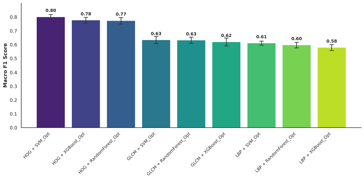
The repeated stratified cross-validation benchmark showed that HOG-based configurations consistently achieved the highest predictive performance among the evaluated descriptors. As shown in

Table 1. Repeated cross-validation benchmark of optimized descriptor-classifier combinations.

Descriptor	Classifier	Accuracy	Macro F1	Macro Precision	Macro Recall	Inference Time (ms/Image)
HOG	SVMOpt	$\mathbf{0.80}\mathbf{\pm }\mathbf{0.02}$	$\mathbf{0.80}\mathbf{\pm }\mathbf{0.02}$	$\mathbf{0.80}$	$\mathbf{0.80}$	$\mathbf{12.45}\mathbf{\pm }\mathbf{0.85}$
HOG	XGBoostOpt	$0.78\pm 0.02$	$0.78\pm 0.02$	$0.78$	$0.78$	$8.12\pm 0.42$
HOG	Random ForestOpt	$0.77\pm 0.02$	$0.77\pm 0.02$	$0.77$	$0.77$	$10.34\pm 0.68$
GLCM	SVMOpt	$0.64\pm 0.03$	$0.63\pm 0.03$	$0.64$	$0.64$	$14.21\pm 1.12$
GLCM	Random ForestOpt	$0.63\pm 0.02$	$0.63\pm 0.02$	$0.63$	$0.63$	$11.05\pm 0.95$
GLCM	XGBoostOpt	$0.62\pm 0.03$	$0.62\pm 0.03$	$0.62$	$0.62$	$9.45\pm 0.53$
LBP	SVMOpt	$0.61\pm 0.02$	$0.61\pm 0.01$	$0.62$	$0.61$	$10.88\pm 0.44$
LBP	Random ForestOpt	$0.60\pm 0.02$	$0.60\pm 0.02$	$0.60$	$0.60$	$9.92\pm 0.61$
LBP	XGBoostOpt	$0.58\pm 0.02$	$0.58\pm 0.02$	$0.58$	$0.58$	$7.56\pm 0.38$

, the best result was obtained with HOG + SVM_Opt, which reached an average accuracy of $0.80\pm 0.02$ and a Macro F1-score of $0.80\pm 0.02$. The second-best configuration was HOG + ${\mathrm{XGBoost}}_{\mathrm{Opt}}$, with a Macro F1-score of $0.78\pm 0.02$. These results indicate that gradient-based morphological information was more discriminative than local texture or second-order gray-level statistics for the evaluated $24\times 40$ pixel thermal images.

The advantage of HOG was observed across the tested classifiers. The best GLCM-based configuration, GLCM + SVM_Opt, reached a Macro F1-score of $0.63\pm 0.03$, whereas the best LBP-based configuration, LBP + SVM_Opt, reached $0.61\pm 0.01$. This supports the interpretation that directional thermal discontinuities are more informative than micro-texture patterns in this low-resolution setting. However, the comparison should be interpreted as an empirical ranking from repeated stratified cross-validation rather than as a formal hypothesis-testing result. Future studies could strengthen this point through paired statistical tests using fold-level scores.

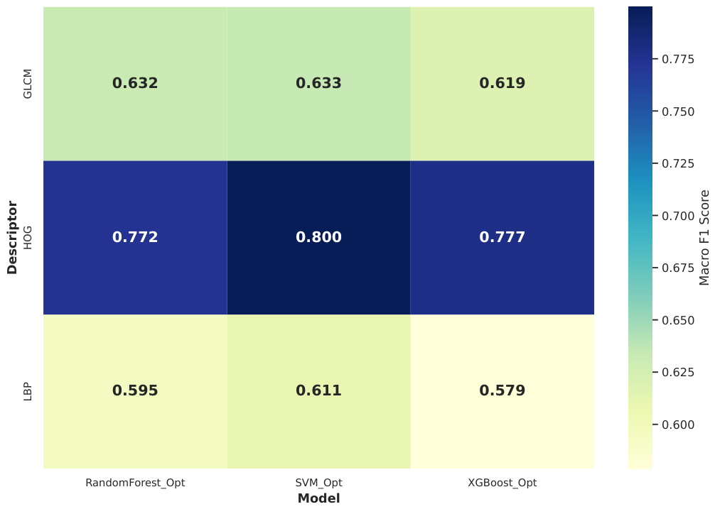
Figure 1 presents the ranking of all configurations in terms of Macro F1 score, while Figure 2 condenses the same information into a descriptor by classifier heatmap. Both representations confirm that the highest predictive performance is concentrated in the HOG family, particularly when paired with the optimized SVM classifier.

3.1. Computational Efficiency and Operational Interpretation

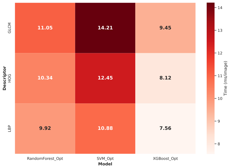
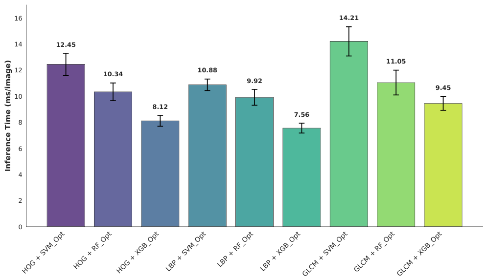
The computational results support the feasibility of the evaluated pipelines for rapid CPU-based screening. HOG + SVM_Opt achieved the best predictive performance with an end-to-end latency of $12.45\pm 0.85$ ms per image, including preprocessing, descriptor extraction, and prediction. Although HOG + XGBoost_Opt was faster, with $8.12\pm 0.42$ ms per image, its Macro F1-score was lower ($0.78\pm 0.02$). In contrast, the fastest LBP and XGBoost configuration reached $7.56\pm 0.38$ ms per image but showed a substantially lower Macro F1-score ($0.58\pm 0.02$).

These results indicate that the best model does not minimize latency alone, but provides the most favorable balance between diagnostic performance and processing cost. From an operational perspective, a Macro F1-score close to $0.80$ is better interpreted as suitable for first-stage screening than as sufficient for autonomous maintenance decisions. The model can help prioritize modules for expert review or higher-resolution inspection, while final decisions should still consider maintenance cost, risk tolerance, and plant-specific operating conditions.

Table 2. Detailed benchmark values for optimized descriptor-classifier combinations under repeated stratified cross-validation.

Descriptor	Classifier	Accuracy	Macro Precision	Macro Recall	Macro F1	Weighted F1	Inference Time (ms/Image)
HOG	SVMOpt	0.80	0.80	0.80	0.80	0.80	12.45
HOG	XGBoostOpt	0.78	0.78	0.78	0.78	0.78	8.12
HOG	Random ForestOpt	0.77	0.77	0.77	0.77	0.77	10.34
GLCM	SVMOpt	0.64	0.64	0.64	0.63	0.63	14.21
GLCM	Random ForestOpt	0.63	0.63	0.63	0.63	0.63	11.05
GLCM	XGBoostOpt	0.62	0.62	0.62	0.62	0.62	9.45
LBP	SVMOpt	0.61	0.62	0.61	0.61	0.61	10.88
LBP	Random ForestOpt	0.60	0.60	0.60	0.60	0.60	9.92
LBP	${\mathrm{XGBoost}}_{\mathrm{Opt}}$	0.58	0.58	0.58	0.58	0.58	7.56

reports the detailed mean values for the optimized descriptor-classifier combinations, including the weighted F1-score used to complement the macro-averaged metrics.

Figure 3 and Figure 4 summarize the end-to-end inference time of the evaluated descriptor-classifier configurations. The bar plot provides a direct latency ranking, whereas the heatmap highlights the latency patterns associated with each descriptor family and classifier.

3.2. Classwise Performance of the Best Global Model

The classwise analysis shown in

Table 3. Classwise results for the HOG + ${\mathrm{SVM}}_{\mathrm{Opt}}$ configuration.

Class	Precision	Recall	F1 Score
Cracking	$0.8421$	$0.8205$	$0.8312$
Hot Spot Multi	$0.7619$	$0.7442$	$0.7529$
No Anomaly	$0.8005$	$0.8300$	$0.8152$
Macro Average	$\mathbf{0.8015}$	$\mathbf{0.7982}$	$\mathbf{0.7998}$

corresponds to the best-performing model, HOG + SVM_Opt. The model showed balanced behavior across the three classes, with F1-scores of $0.8312$ for Cracking, $0.7529$ for Hot Spot Multi, and $0.8152$ for No Anomaly. The lowest classwise performance was observed for Hot Spot Multi, consistent with the partial overlap between distributed hotspot patterns and moderate temperature gradients in healthy panels. The Cracking class obtained the highest precision ($0.8421$), suggesting a low false-positive tendency for crack-related signatures in the evaluated dataset.

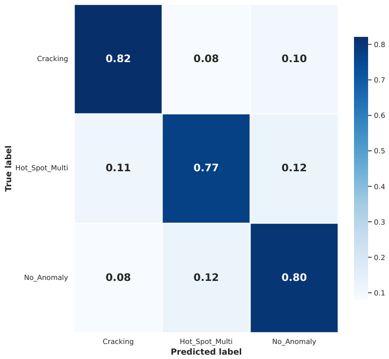
The normalized confusion matrix shown in Figure 5 confirms this balanced behavior for the HOG + SVM_Opt model. The diagonal terms were dominant for all classes, with correct classification rates of $0.82$ for Cracking, $0.74$ for Hot Spot Multi, and $0.83$ for No Anomaly. The main confusion occurred between Hot Spot Multi and No Anomaly, which is expected because mild distributed heating can resemble normal thermal gradients in low-resolution images. This pattern confirms that the model provided reasonable separation among the three classes, while also showing where additional data or higher-resolution inspection could improve reliability.

3.3. Qualitative Interpretation of Descriptor Responses

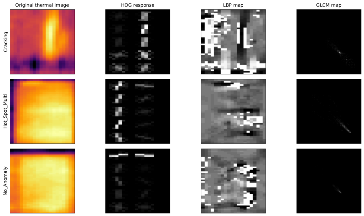
The qualitative descriptor visualization in Figure 6 helps explain the numerical ranking. HOG highlights directional gradients and boundary transitions, which are relevant for cracks and compact hotspot regions. This behavior is consistent with the higher Macro F1-score obtained by HOG-based models, especially HOG + SVM_Opt.

LBP captures local micro-texture variations, but its response is less aligned with the global geometry of the defects. GLCM summarizes second-order gray-level relationships, which reduces dimensionality but also removes spatial specificity. These differences explain why LBP and GLCM were less competitive than HOG in the evaluated low- resolution images.

The higher performance of HOG compared with LBP and GLCM can be explained, in part, by the severe spatial constraint imposed by the native $24\times 40$ pixel resolution. Under this condition, descriptors based on local micro texture or pixel-level statistical variation, such as LBP and GLCM, lose discriminative capacity because fine thermal details are weakly represented. HOG is less affected by this limitation because it aggregates gradient magnitudes and orientations over local cells and blocks, preserving the dominant boundary information and directional thermal discontinuities associated with cracks and hotspot patterns. The results support three methodological findings. First, useful automated diagnosis can be achieved from very low-resolution photovoltaic thermograms when the feature representation captures spatial gradients effectively. Second, predictive performance depends more strongly on descriptor design than on classifier complexity, although the optimized SVM provided a robust nonlinear decision boundary that improved the separation of HOG features compared with the ensemble models. Third, the best performing configuration maintained an end to end inference time below 15 ms per image, which supports its practical relevance for edge oriented inspection. The classwise results also show that the best global model remained balanced across the three categories, indicating that the detection of structural defects such as cracking was not achieved at the expense of healthy panel or hotspot recognition. Taken together, these findings support HOG + SVM_Opt as the most suitable descriptor classifier pair among the evaluated configurations for low resolution infrared inspection of photovoltaic panels, offering the best balance between diagnostic reliability and computational efficiency.

4. Conclusions

This study showed that low-resolution infrared images can support automated thermal anomaly detection in photovoltaic modules when the feature representation preserves the spatial structure of the thermal field. Among the evaluated configurations, HOG + SVM_Opt provided the best balance between predictive performance and computational cost. In repeated stratified cross-validation, this configuration achieved a Macro F1-score of $0.80\pm 0.02$ and an accuracy of $0.80\pm 0.02$ using native $24\times 40$ pixel images.

The best-performing model also maintained an end-to-end CPU latency of $12.45\pm 0.85$ ms per image, including preprocessing, descriptor extraction, and prediction. This result supports its use as a lightweight, interpretable screening tool to prioritize PV modules for expert review or higher-resolution inspection. Since no lightweight CNN baseline was included, the findings should be interpreted as evidence of the proposed shallow pipeline’s suitability on the evaluated dataset, rather than as a direct comparison with deep neural architectures.

The study has several limitations. The benchmark was restricted to three classes and a single public dataset, and the available metadata did not permit module-disjoint validation. In addition, the balanced sampling strategy does not reproduce the field prevalence, in which healthy modules generally dominate. Environmental and operational factors such as irradiance, ambient temperature, wind speed, emissivity, soiling, viewing angle, and module loading may also modify the appearance of thermal anomalies. Future work should therefore evaluate heterogeneous field datasets, module-disjoint and plant-disjoint validation, imbalanced operating conditions, feature-fusion strategies, multi-scale descriptors, additional shallow classifiers, and lightweight CNN baselines under the same hardware-aware latency protocol.