A Novel Hybrid Neural Network with Optimized Feature Selection for Spindle Thermal Error Prediction

Abstract

In modern intelligent manufacturing, spindle thermal errors are critical to machining accuracy. To address this, we propose a two-stage prediction framework. First, for feature selection, an enhanced Red-Billed Magpie Optimization algorithm (RBMO-X) optimizes the parameters of a hybrid convolutional neural network (DLTK). Concurrently, PSO-optimized HDBSCAN clustering combined with Pearson correlation selects optimal temperature-sensitive points. The DLTK network integrates LSTM, deformable convolution, Transformer, and Fourier KAN modules for robust spatiotemporal feature extraction. The experimental results demonstrate significant improvements. The proposed feature selection method improves the Silhouette index by 32.39% and increases BWP by 49.16%. Using the selected points reduces prediction RMSE by 31.89% compared to random selection. The final RBMO-X-DLTK model achieves an RMSE of 0.181 μm, an MAE of 0.128 μm, and an R² score of 0.9978, outperforming seven benchmark models (e.g., BP, LSTM, CNN-LSTM). In practical validation, the model enabled an average thermal error reduction of 89%. This integrated approach provides a robust and accurate solution for spindle thermal error prediction, demonstrating strong generalization capability.

1. Introduction

The transition to intelligent manufacturing demands higher machining accuracy. As the core component of CNC machine tools, the motorized spindle is a primary source of thermal error, accounting for 40%~70% of the total machining error [1,2,3]. During prolonged operation, the motorized spindle experiences significant temperature increases, which degrade machining accuracy and escalate maintenance and operational costs. Consequently, the ability to accurately predict and compensate for the thermal error of motorized spindles has emerged as a critical challenge in enhancing machining precision.

Thermal error compensation is an effective method to mitigate the impact of thermal errors and enhance the machining accuracy of machine tools [4,5,6]. Reducing redundancy and collinearity in temperature data while developing a thermal error prediction model with high precision and robustness is critical for successfully implementing thermal error compensation techniques. Although prediction model technologies have progressed, accurately predicting thermal errors remains challenging due to the complex nonlinear relationships between multiple temperature points and spindle thermal behavior. Existing models often struggle to capture these complexities or require substantial computational resources, making it difficult to balance predictive performance and computational efficiency.

Currently, researchers have conducted extensive studies on thermal error prediction and compensation techniques for motorized spindles [7,8,9,10], with physical modeling and data-driven methods dominating the field. Physical modeling methods rely on an in-depth understanding of heat source distribution, heat transfer mechanisms, and environmental conditions, providing an explanation for the mechanisms of thermal error generation and being suitable for relatively simple operating conditions [11]. However, the applicability of such methods is significantly limited under dynamic and complex working conditions. In contrast, data-driven methods build predictive models by learning patterns from experimental data without explicitly establishing heat transfer equations, demonstrating robust nonlinear modeling capabilities [12,13,14]. In recent years, the rapid advancement of deep learning has led to its widespread adoption in the industrial field [15,16,17]. Neural network-based thermal error prediction models have gained attention, excelling in predictive accuracy due to their strong capabilities in modeling temporal and spatial features. However, existing data-driven methods still face several challenges: the selection of temperature points often relies on manual experience or simple statistical methods, resulting in redundant input features, hyperparameter tuning is inefficient, increasing the computational cost of the models [18,19,20,21]. Furthermore, the generalizing ability and stability of the models under multiple operating conditions need further improvement.

This study makes three primary contributions to spindle thermal error prediction modeling. First, regarding feature selection, this combination is specifically employed because HDBSCAN can effectively identify clusters of varying density and isolate noise in temperature field data, while PSO efficiently optimizes its key parameters to ensure the selected temperature clusters exhibit maximum correlation with the thermal error. By combining particle swarm optimization and adaptive density clustering, this method successfully identifies the temperature points most significantly affecting thermal error, effectively reducing temperature data redundancy and enhancing the quality of input features. Second, regarding model architecture and optimization, to efficiently optimize the hyperparameters of the complex DLTK network, this study develops the RBMO-X-DLTK hybrid convolutional neural network model, which employs the RBMO-X algorithm—an enhanced optimizer designed for robust global search and stable convergence in high-dimensional spaces. The DLTK network integrates multiple advanced modules (e.g., 1D deformable convolution, LSTM, Transformer, Fourier KAN) for comprehensive feature extraction. The proposed RBMO-X optimizer is novel for its hybrid design, integrating deep learning training stabilizers (SGDR scheduler and gradient clipping) directly into the metaheuristic loop (see Section 4.1), which enables stable tuning and contributes to the model’s superior performance, such as a >30% reduction in RMSE compared to benchmarks. Third, as the integrated outcome, the core innovation of this paper lies in proposing and validating a novel, integrated pipeline that systematically addresses the need for efficient feature selection and an optimized, robust predictive model by combining an optimized temperature-sensing strategy with a specially designed and optimized hybrid neural network, thereby achieving superior accuracy and robustness in spindle thermal error prediction.

The remainder of the paper is organized as follows: Section 2 introduces related works. Section 3 proposes a temperature selection method based on PSO-optimized HDBSCAN. Section 4 presents the RBMO-X optimized DLTK hybrid neural network. Section 5 details the experimental setup, analyzes the performance of temperature point selection and optimization, and compares the results with other models. Section 6 validates the model through real-world compensation experiments. Section 7 discusses the experimental results in detail. Section 8 concludes this study and suggests potential future work.

2. Related Work

Efficient selection of temperature points highly correlated with thermal errors is critical for enhancing the performance of prediction models. In recent years, researchers have conducted extensive studies on temperature point selection, the application and optimization of deep learning, and adaptability under dynamic conditions. Early temperature point selection methods focused on improving clustering algorithms, such as K-Harmonic Means (KHM) [22] Correlation Coefficient Variation Determination Factor (CCVDF) [23], and Synthetic Temperature Information (STI) [24] While these methods improved selection accuracy to some extent, they often suffer from sensitivity to initial conditions, weak adaptability to dynamic conditions, or high computational complexity, limiting their real-time application.

The introduction of optimization algorithms, such as the Binary Bat Algorithm (BBA) [25] and the Improved Binary Grasshopper Optimization Algorithm (IBGOA) [26], marked a breakthrough by directly optimizing feature subsets for prediction accuracy. However, these methods often struggle with computational efficiency in high-dimensional spaces or tend to converge to local optima, leading to unstable selection results.

While the aforementioned studies have advanced the field, they reveal several common challenges. Methods based on static statistical analysis or conventional clustering often lack adaptability to dynamic thermal conditions and may select redundant or pseudo-correlated points. Although optimization algorithms improve accuracy, they can suffer from high computational cost in high-dimensional spaces or a tendency to converge to local optima, leading to unstable selection results. Furthermore, the selection process is often decoupled from the final prediction model, lacking a unified optimization objective.

The development of deep learning has brought groundbreaking advancements to thermal error modeling. For example, Zhao et al. [27] invented a thermal error prediction method for the ball screw feed system of CNC machine tool, capable of predicting the heat generation rate, temperature distribution, and thermal error of the ball screw feed drive system. The proposed Adaptive Real-Time Model (ARTM) can predict the thermal error of the ball screw feed drive system but has limitations in addressing the complexity of spindle thermal error. To enhance model performance, researchers have begun exploring the integration of deep learning and optimization algorithms. For instance, Li et al. [28] optimized BP neural network parameters using Improved Particle Swarm Optimization (IPSO), which improved prediction accuracy but still faced issues such as high computational complexity and a tendency to fall into local optima. To overcome these shortcomings, Li et al. [29] proposed the Beetle Antennae Search (BAS) algorithm to optimize BP neural network-based thermal error prediction models for motorized spindles. Experiments confirmed that BAS-BP models achieved higher prediction accuracy than BP and GA-BP models at different speeds. However, these methods primarily focus on single-model optimization, neglecting systematic studies on input feature selection and adaptability to dynamic conditions. To address this, Li et al. [30] further proposed an optimized Extreme Learning Machine (MPA-ELM) based on the Marine Predators Algorithm, designed to predict thermal displacement in motorized spindle models. They compared the accuracy of ELM, MPA-ELM, and GA-ELM (Genetic Algorithm-optimized ELM). Experimental data demonstrating that MPA-ELM achieved superior prediction accuracy. However, the issue of low efficiency in input feature selection persists.

To enhance the adaptability and robustness of deep learning models under dynamic conditions, Gao et al. [31] optimized the LSTM network using PSO, significantly improving the predictive performance of thermal error models. Compared to traditional RBF and BP models, the PSO-LSTM model demonstrated superior accuracy and robustness, particularly in environments with strong nonlinear dynamic characteristics. However, as model complexity increases, this method becomes heavily reliant on hyperparameter selection, limiting its scalability under diverse dynamic conditions. To further address the limitations of temperature point selection under dynamic conditions, Du et al. [32] developed a thermal error prediction model based on temperature-sensitive point recognition using an attention mechanism. This model adaptively focuses on the importance of different temperature points, avoiding the drawbacks of traditional methods that rely on manual temperature point selection and significantly improving prediction flexibility. However, due to the complex computation of the attention mechanism, this method is less adaptable to scenarios with high real-time requirements, and the interpretability of attention weights requires further investigation. Wu et al. [33] utilized CNNs combined with thermal images and thermocouple data to model and predict the temperature field under dynamic conditions, demonstrating high accuracy and robustness. However, this method relies on high-quality thermal image input, making it susceptible to image noise and hardware device accuracy, which limits its application in low-cost environments. To address the spatiotemporal characteristics of thermal error, Guo et al. [34] proposed a Spatiotemporal Correlation Hybrid Model (ST-CLSTM) based on CNN and LSTM. However, this method faces a risk of performance degradation when handling long time series and is heavily reliant on hyperparameter tuning.

In the direction of model optimization, Gao et al. [35] utilized the Pelican Optimization Algorithm (POA) to optimize the CNN-LSTM model, enhancing its performance under multiple working conditions. The introduction of POA effectively improved the model’s adaptability and robustness under complex conditions. However, due to the algorithm’s random search characteristics, its convergence speed is slow, reducing its efficiency in large-scale data scenarios. Additionally, Li et al. [36] proposed GWO-LSSVM thermal error modeling, which exhibited higher accuracy and modeling efficiency compared to traditional models. However, this method primarily focuses on static conditions and is sensitive to input feature fluctuations under dynamic conditions, limiting its performance in practical applications. To address these issues, Fu et al. [37] proposed thermal error modeling based on CNN optimized by the Mayfly Algorithm, achieving accurate spindle thermal error prediction under various conditions. Experiments showed that this method performed well under various conditions, but balancing selection efficiency and prediction performance when handling high-dimensional feature data requires further optimization. For modeling in complex dynamic environments, Yang et al. [38] proposed a CNN-GRU model combined with a Subtractive Averaging Based Optimizer (SABO). It demonstrated superior performance across multiple error metrics (e.g., MAE, RMSE). However, as model complexity increased, training time significantly extended, and the high preprocessing requirements for input data increased the deployment cost. Meanwhile, Dai et al. [39] proposed a CS-Elman model optimized by the Cuckoo Search algorithm, which further improved prediction stability. However, the CS-Elman model has high computational complexity, and the local search capability of the algorithm limits further model improvements.

Despite their success, existing deep learning models for thermal error prediction exhibit notable shortcomings. Models that heavily rely on manual hyperparameter tuning incur significant computational overhead. While complex hybrid architectures capture spatiotemporal features, their performance is sensitive to input fluctuations and often requires extensive data preprocessing. Moreover, many studies focus on either improving the model architecture or the input features, neglecting the synergistic potential of co-optimizing both within an end-to-end framework.

Most recently, research in 2025 has begun to emphasize the need for integrated solutions that concurrently address efficient feature selection and robust, adaptive model design to tackle the complex spatiotemporal characteristics of thermal error under dynamic conditions [40]. This trend toward co-design highlights the importance of a systematic pipeline but also indicates that achieving an optimal balance between accuracy, efficiency, and generalization remains an open challenge.

In summary, significant progress has been made in motorized spindle thermal error modeling in areas such as temperature point selection, deep learning model optimization, and adaptability to dynamic conditions. However, a critical synthesis of the literature, informed by the limitations discussed above, reveals three interconnected research gaps that limit the development of a robust and efficient prediction system:

(1)

Existing methods exhibit a trade-off between selection efficiency and accuracy when handling high-dimensional complex feature data, failing to fully capture the nonlinear relationships between temperature points and thermal errors. Additionally, some optimization algorithms are prone to local optima in large-scale data scenarios, leading to unstable selection results.

(2)

While deep learning methods (e.g., LSTM, CNN-LSTM, ST-CLSTM) have demonstrated excellent performance in thermal error modeling, there is still significant room for improvement in module collaboration and hyperparameter optimization. The design and tuning of complex models often require substantial computational resources, increasing the difficulty of practical applications.

(3)

Existing models achieve high predictive accuracy under specific conditions but lack adaptability under multi-condition scenarios. In particular, their predictive performance is highly susceptible to input feature fluctuations in dynamic thermal environments.

This study is designed to bridge these specific gaps cohesively. The integration of metaheuristic optimization algorithms with clustering techniques, such as PSO with K-Means or GA with DBSCAN, has been explored in other fields for feature selection and pattern recognition. However, within the specific domain of motorized spindle thermal error modeling, the tailored integration of PSO with HDBSCAN for optimal temperature-sensitive point selection remains underexplored. This gap is notable because the PSO-HDBSCAN combination is particularly suited to address the aforementioned challenges: HDBSCAN’s ability to identify clusters of varying density and reject noise directly tackles the issue of redundant and pseudo-correlated temperature points under dynamic conditions, while PSO’s parameter optimization ensures the clustering outcome is explicitly guided by thermal error correlation, enhancing selection efficiency and accuracy. Therefore, proposing and validating this tailored pipeline for spindle thermal error prediction constitutes a novel and necessary contribution to the field. Addressing these issues requires an efficient and robust temperature point selection method, along with a deep learning modeling and optimization strategy that balances accuracy and efficiency, which is the focus of this study. The proposed PSO-HDBSCAN method effectively achieves efficient temperature point selection. Additionally, the RBMO-X-DLTK model proposed in this study optimizes the hyperparameters of DLTK using RBMO-X, further enhancing the model’s predictive accuracy and computational efficiency. This combined approach, therefore, constitutes a novel and integrated solution that directly addresses the gaps in efficient feature selection, optimized model architecture, and systemic integration, offering a robust and efficient pipeline for spindle thermal error prediction.

3. PSO-HDBSCAN Temperature Point Selection Method

To address the temperature point selection problem, we propose a novel PSO-HDBSCAN method. It leverages Particle Swarm Optimization (PSO) to optimize the key parameters of the HDBSCAN clustering algorithm, ensuring the selected temperature points are highly correlated with thermal error while minimizing data redundancy.

Particle Swarm Optimization (PSO) is a swarm-intelligence-based global optimizer for complex multi-dimensional problems [41,42,43]. PSO is chosen for its efficiency in continuous parameter optimization and stable convergence properties, which are well suited for this task. The standard PSO procedure adapted for our parameter tuning is outlined in Algorithm 1.

Algorithm 1 PSO (${\mathit{x}}_{\mathit{i}}$, ${\mathit{v}}_{\mathit{i}}$, $\mathit{p}\mathit{B}\mathit{e}\mathit{s}{\mathit{t}}_{\mathit{i}},\mathit{g}\mathit{B}\mathit{e}\mathit{s}\mathit{t}$)

1:  Initialize_Swarm:

2:     for each particle i$= 1$ to $N$ do

3:      $x_i \leftarrow random\_position\left(\right)$

4:      $v_i$ ← random_velocity ()

5:      $pBes{t}_i \leftarrow x_i$

6:      $f_i \leftarrow evaluate\_fitness\left(x_i\right)$

7:     end for

8:     $gBest \leftarrow {argmax}_i\left(f_i\right)$

9:  while termination criterion not met do

10:     for each particle $i =$ $1$ to $N$ do

11:      Update_Velocity_Position:

12:        $v_i \leftarrow \omega ·v_i + c1·rand\left(\right)·(pBes{t}_i - x_i) + c2·rand\left(\right)·(gBest - x_i)$

13:        $x_i \leftarrow x_i + v_i$

14:      $Evaluate\_Fitness:$

15:        $f_{\mathit{current}} \leftarrow evaluate\_fitness\left(x_i\right)$

16:      if $f_{\mathit{current}} > f_i$ then

17:      $Update\_Best:$

18:        $pBes{t}_i \leftarrow x_i$

19:        $f_i \leftarrow f_{\mathit{current}}$

20:      end if

21:     end for

22:     $Update\_Best:$

23:      $gBest \leftarrow {argmax}_i\left(f_i\right)$

24:  end while

25:  return $gBest$

Algorithm 1 details the standard Particle Swarm Optimization (PSO) procedure. It operates on a swarm of candidate solutions (particles), where each particle $i$ has a position $x_i$ (a potential solution in the search space) and a velocity $v_i$. The algorithm maintains two key memory traces for each particle: its personal best position to date ($pBes{t}_i$) and corresponding best fitness ($f_i$). while the swarm shares a global best position ($gBest$). found by any particle. The core iteration (Lines 10–25) updates each particle’s velocity by combining its previous momentum (weighted by inertia coefficient $\omega$), a cognitive component toward $pBes{t}_i$, and a social component toward $gBest$ (Line 13). The new position is then computed (Line 14), and after evaluating its fitness (Line 16), $pBes{t}_i$ and $gBest$ are updated if improvements are detected (Lines 18–20, 23–24). This process repeats to drive the swarm toward promising search space regions until a termination criterion is satisfied.

HDBSCAN is an improved version of DBSCAN [44], a density-based clustering algorithm, automatically determines the number of clusters and identifies noise. This makes it suitable for adaptive selection of temperature-sensitive points from our dataset. Its procedure is detailed in Algorithm 2.

Algorithm 2 HDBSCAN ($\mathit{core}\_\mathit{k}\left(\mathit{p}\right)$, $\mathit{M}\mathit{S}\mathit{T}$, hierarchy)

1:  $Compute\_Core\_Distance:$

2:     for each point $p$ in data points $P$ do

3:    ${\mathit{core}}_k\left(p\right) \leftarrow$ distance to k-th nearest neighbor of $p$

4:     end for

5:  $Build\_MST:$

7:     for each pair of points $(p, q)$ do

8:    $d_{mreach}(p,q) \leftarrow max\left({\mathit{core}}_k\right(p), {\mathit{core}}_k(q), dist(p, q\left)\right)$

9:     end for

10:   Construct graph $G$ where edge weight $=$ $d_{mreach}(p,q)$

11:   $MST \leftarrow minimum\_spanning\_tree\left(G\right)$

12:  $Form\_Tree:$

13:   hierarchy $\leftarrow$ $convert\_mst\_to\_dendrogram\left(MST\right)$

14:  $Extract\_Clusters:$

15:   clusters, noise $\leftarrow extract\_flat\_clusters\_from\_dendrogram\left(hierarchy\right)$

16:  return clusters, noise

Algorithm 2 details the HDBSCAN procedure for clustering temperature points. It first computes the core distance ${\mathit{core}}_k\left(p\right)$ for each point $p$ to measure local density (Lines 1–4). Using these, the mutual reachability distance $d_{mreach}(p,q)$ between every point pair $(p, q)$ is calculated to form a density-adjusted graph, from which a minimum spanning tree ($MST$) is built (Lines 7–11). The $MST$ is then converted into a hierarchical cluster tree (hierarchy) (Lines 12–13). Finally, the most stable clusters are extracted from this hierarchy, while remaining points are labeled as noise (Lines 14–16). This process automatically identifies groups of points with similar density and separates outliers, effectively reducing redundancy and selecting representative temperature-sensitive points for the thermal error model.

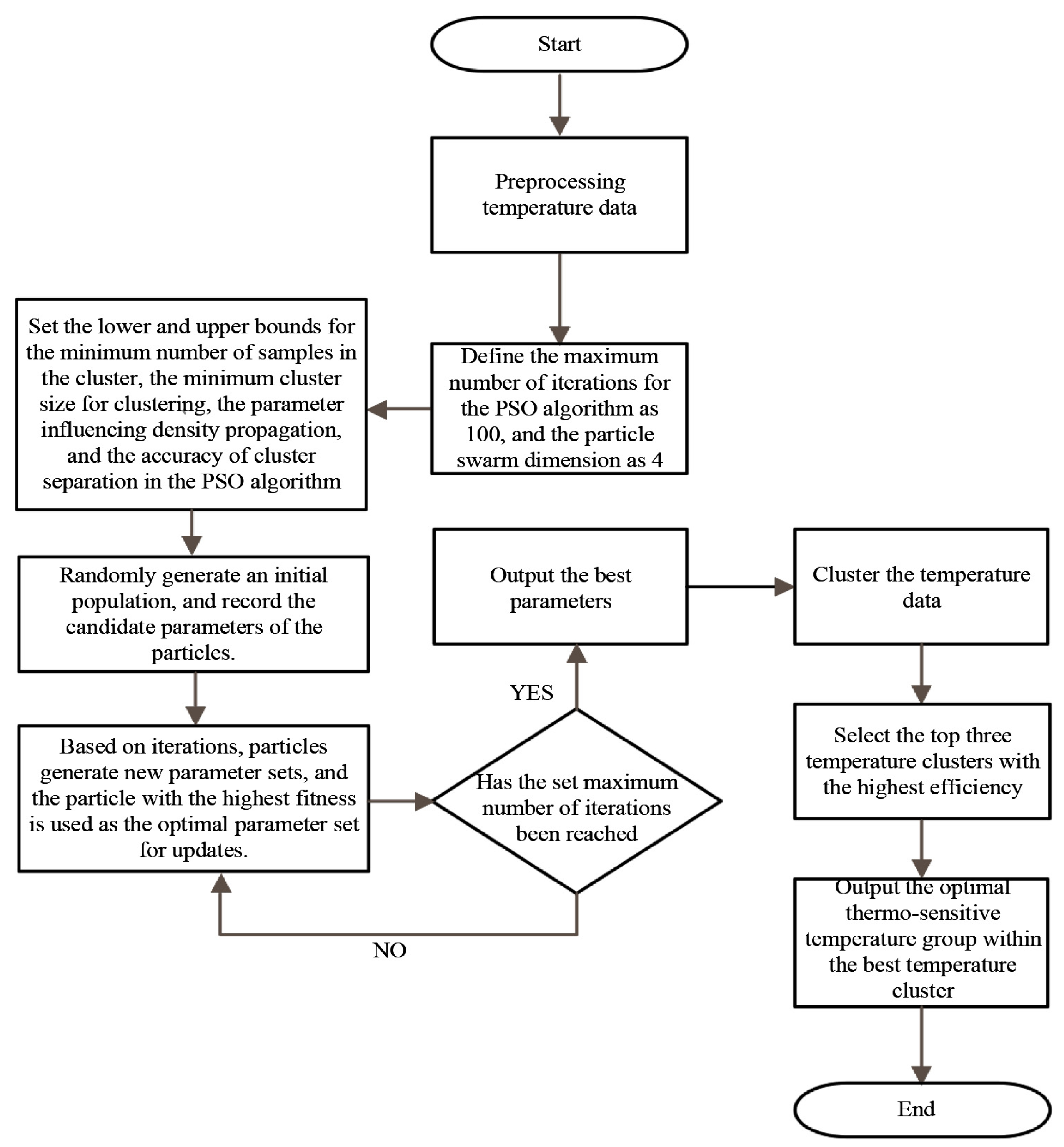
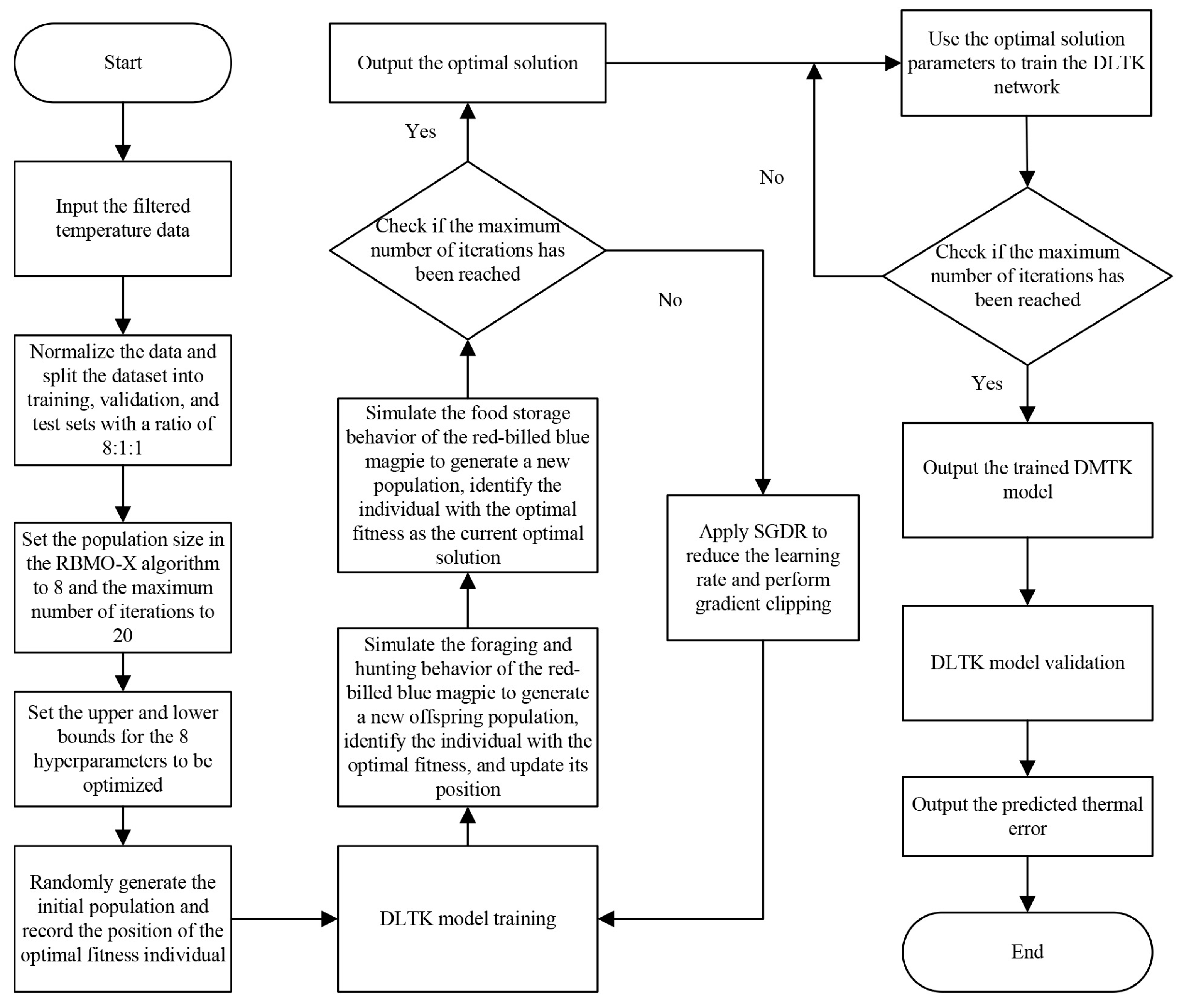
The PSO-HDBSCAN integration dynamically optimizes key HDBSCAN parameters (e.g., minimum samples, cluster size) to maximize the correlation between identified temperature clusters and the thermal error. This integrated process, illustrated in Figure 1, is formalized in Algorithm 3.

Algorithm 3 PSO-HDBSCAN (${\mathit{\theta }}_{\mathit{i}}$, ${\mathit{v}}_{\mathit{i}}$, $\mathit{p}\mathit{B}\mathit{e}\mathit{s}{\mathit{t}}_{\mathit{i}}, \mathit{g}\mathit{B}\mathit{e}\mathit{s}\mathit{t},{\mathit{\theta }}^{\mathit{*}},$ ${\mathit{C}}^{\mathit{*}})$

1:  Initialize:

2:   $Set M, N, \omega , c1, c2.$

3:   Define parameter bounds $\Omega .$

4:   for $i = 1 to N$ do

5:      ${\theta }_i \leftarrow RandomInit\left(\Omega \right)$

6:      $v_i \leftarrow RandomInit\left(\right)$

7:      $pBest\_i \leftarrow {\theta }_i$

8:      $f_i \leftarrow Fitness\left({\theta }_i\right)$

9:   end for

10:    $gBest \leftarrow {argmax}_i\left(f_i\right)$

11:    $k \leftarrow 0$

12:   while $k < M$ do

13:  for $i = 1 to N$ do

14:      $Evaluate:$

15:        $C_i \leftarrow HDBSCAN(T, {\theta }_i)$

16:         $f_i\leftarrow {max}_{\{C \in C_i\} Pearson(C, E)}$

17:      $Update\_Best:$

18:         if $f_i > Fitness\left(pBes{t}_i\right)$ then $pBes{t}_i \leftarrow {\theta }_i$

19:         if $f_i > Fitness\left(gBest\right)$ then $gBest \leftarrow {\theta }_i$

20:      $Update\_Swarm:$

21:         $v_i \leftarrow \omega \ast v_i + c1 \ast r1 \ast (pBes{t}_i - {\theta }_i)$

22:        $+ c2 \ast r2 \ast (gBest - {\theta }_i)$

23:         ${\theta }_i \leftarrow {\theta }_i + v_i$

24:         ${\theta }_i \leftarrow Clip({\theta }_i, \Omega )$

25:  end for

26:   $k \leftarrow k + 1$

27:  end while

28:  ${\theta }^{*} \leftarrow gBest$

29:  $C^{*} \leftarrow HDBSCAN(T, {\theta }^{*})$

30:  return ${\theta }^{*}$, $C^{*}$

Algorithm 3 describes the integrated PSO-HDBSCAN optimization. The swarm is initialized with random HDBSCAN parameters (lines 4–11). In each iteration, every particle’s position (a parameter set) is used to cluster the temperature data via HDBSCAN, and the fitness is computed as the maximum Pearson correlation between any cluster and the thermal error (lines 15–17). Personal and global best positions are updated if higher fitness is found (lines 19–21). The swarm then updates velocities and positions via standard PSO equations, with parameters bounded within the search space $\Omega$ (lines 23–28). After $M$ iterations, the algorithm returns the optimal parameter set ${\theta }^{*}$ and the corresponding temperature cluster $C^{*}$ (lines 28–30). This pipeline systematically tunes HDBSCAN to select the most representative temperature-sensitive points.

The PSO-HDBSCAN framework mitigates the sensitivity of manual parameter tuning by dynamically optimizing HDBSCAN parameters. The optimization is guided by a fitness function that directly maximizes the Pearson correlation between temperature clusters and thermal error, ensuring the selection is objective and data-driven. Reasonable search bounds for the parameters are defined in Section 5.1.

4. RBMO-X-DLTK Thermal Error Modeling Method

Building upon the optimally selected temperature points from PSO-HDBSCAN, this section presents the RBMO-X-DLTK hybrid neural network model for thermal error prediction. The model consists of the DLTK network for spatiotemporal feature extraction and the RBMO-X optimizer for hyperparameter tuning. This combined approach leverages precise inputs and optimized architecture to enhance prediction accuracy and robustness.

4.1. RBMO-X Optimization Algorithm

Optimizing the hyperparameters of the complex DLTK network requires a robust global search algorithm. We select the Red-billed Blue Magpie Optimization (RBMO) as the foundation for its effective collaborative search strategy. The original RBMO algorithm mimics red-billed blue magpies’ foraging and hunting behaviors, offering certain global search capabilities [45,46]. However, in high-precision spindle thermal error prediction, RBMO faces limitations in multi-dimensional hyperparameter search, primarily exhibiting slow convergence and insufficient global exploration, making it prone to local optima. Particularly in thermal error prediction induced by temperature fluctuations, RBMO demonstrates slow convergence and instability issues, limiting its effectiveness in this complex prediction task.

To directly overcome the aforementioned limitations, this section improves the RBMO algorithm and proposes the RBMO-X algorithm. The algorithm enhances global search stability and convergence precision by incorporating a Stochastic Gradient Descent with Restarts (SGDR) learning rate scheduler and gradient clipping techniques [47,48]. The RBMO-X algorithm is particularly suited for hyperparameter optimization of the DLTK network, significantly improving model training efficiency and prediction accuracy. The main innovations of the RBMO-X algorithm include the following three aspects:

(1)

RBMO-X integrates the collaborative search of small and large groups, enabling it to quickly identify critical parameter regions while fine-tuning to achieve optimal hyperparameter configurations in predictive model optimization. Small groups explore local spaces, while large groups cover a broader search range, ensuring the model efficiently captures the dynamic nonlinear patterns of spindle thermal error under multi-temperature point inputs and high-dimensional data features.

(2)

RBMO-X incorporates the SGDR cosine annealing learning rate mechanism, dynamically adjusting the learning rate during training to avoid local optima in fitting high-dimensional nonlinear thermal error data, thereby ensuring stable model convergence. This dynamic scheduling is implemented using Equation (1):

$${\eta }_t={\eta }_{min}+{\displaystyle \frac{1}{2}}\left({\eta }_{max}-{\eta }_{min}\right)\left(1+cos\left({\displaystyle \frac{T_{cur}}{T_{max}}}\cdot \mathsf{\pi }\right)\right)$$

(1)

where ${\eta }_t$ is the learning rate at the current training step $t$, ${\eta }_{min}$ is the minimum learning rate, defining the lowest learning rate at the end of the cosine annealing process, when the value of the cosine function is at its minimum, approaching or reaching ${\eta }_{min}$, ${\eta }_{max}$ is the maximum learning rate, representing the initial learning rate or the learning rate at the beginning of each cycle, $T_{cur}$ denotes the current training step (or time step), and $T_{max}$ represents the total number of training steps within the current cycle.

This mechanism effectively assists the DLTK network in gradually converging, enhancing the model’s generalization ability and ensuring the accuracy of thermal error predictions under complex multi-dimensional temperature data.

(3)

In the process of spindle thermal error prediction, data fluctuations, and high-dimensional characteristics can easily cause gradient explosion, affecting model stability. RBMO-X mitigates this issue by applying gradient clipping to limit the L2 norm of gradients, ensuring the stability of the update process. This mechanism constrains excessively large gradient values during each update, enhancing training safety and convergence speed, and enabling the DLTK network to effectively avoid overfitting during long training sessions.

Therefore, the proposed RBMO-X distinguishes itself from the original RBMO and other metaheuristics through a hybrid design that embeds deep learning training stabilizers—the SGDR scheduler and gradient clipping—directly into its search loop. This integration provides the convergence stability essential for tuning complex networks like DLTK, a capability typically absent in standard swarm-based algorithms.

To clearly present the workflow of the RBMO-X algorithm, its key steps are summarized in Algorithm 4 below.

Algorithm 4 RBMO-X (${\mathit{\varphi }}_{\mathit{i}}$, ${\mathit{f}}_{\mathit{i}}$, ${\mathit{p}}_{\mathit{i}},{\mathit{\Gamma }}_{\mathit{S}\mathit{G}},{\mathit{\Gamma }}_{\mathit{L}\mathit{G}},$ ${\mathit{\varphi }}^{\mathit{*}},\mathit{\Psi })$

1:  Initialize:

2:  $Set \Psi ,{\varphi }^{*}.$

3:  for $i = 1 to N$ do

4:     ${\varphi }_i \leftarrow RandomInit\left(\Omega \right)$

5:  end for

6:  $SG, LG \leftarrow Divide\_Population\left(\Phi \right)$

7:  for $i = 1 to N$ do

8:     $f_i \leftarrow Evaluate\_Fitness\left({\varphi }_i\right)$

9:     $p_i$ ←${\varphi }_i$

10:  end for

11:  ${\Gamma }_{SG}$, ${\Gamma }_{LG}$ ← $Find\_Group\_Bests(SG, LG, f)$

12:  $\Psi \leftarrow {argmax}_i\left(f_i\right)$

13:  $t \leftarrow 0$

14:  for $k = 1 to M$ do

15:     for each group in $\{SG, LG\}$ do

16:       for each magpie $i$ in group do

17:        ${\Phi }_i^{\prime }$ ← $RBMO\_Foraging\_Strategy({\varphi }_i, p_i, {\Gamma }_{group})$//Core search [31]

18:        $f_i^{\prime }$ $\leftarrow Evaluate\_Fitness({\Phi }_i^{\prime }, t)$

19:        if $f_i^{\prime }$ > $f_i$ then

20:          ${\varphi }_i$ $\leftarrow {\Phi }_i^{\prime }$

21:          $f_i \leftarrow f_i^{\prime }$

22:          $p_i$ $\leftarrow {\varphi }_i$

23:        end if

24:       end for

25:       Update group best ${\Gamma }_{group}$

26:     end for

27:     for each magpie $i$ do

28:        Compute learning rate ${\eta }_t$ according to Equation (1)

29:        ${\varphi }_i \leftarrow {\varphi }_i + {\eta }_t \ast V_i$//$V_i$ is the update vector from line 17

30:     end for

31:     Update global best $\Psi$

32:     $t \leftarrow t + 1$

33:  end for

34:  return $\Psi$ as ${\varphi }^{*}$

Algorithm 4 delineates the workflow of the RBMO-X algorithm, whose core innovation is the deep integration of the SGDR learning rate scheduler (Equation (1)) and gradient clipping technique into the RBMO framework. The algorithm begins by initializing the hyperparameter population (individuals denoted as ${\varphi }_i$) and dividing it into groups ($SG, LG$). In the main loop, each individual generates a candidate solution ${\Phi }_i^{\prime }$ via the RBMO strategy (line 17). The evaluation of its fitness $f_i^{\prime }$ (line 18) internally embeds the DLTK network training that employs the SGDR learning rate ${\eta }_t$ and gradient clipping, ensuring optimization stability. If the candidate is superior, the current solution ${\varphi }_i$ and the personal best $p_i$ are updated (lines 19–23). Subsequently, all individuals scale their update vector $V_i$ using the computed ${\eta }_t$ to perform the position update (lines 28–29). The algorithm finally returns the global best solution $\Psi$ as the optimal hyperparameter set ${\varphi }^{*}$.

4.2. DLTK Hybrid Convolutional Neural Network

For spindle thermal error prediction, this section designs a hybrid convolutional neural network model DLTK, see Figure 2, The architecture is deliberately constructed as a complementary, hierarchical pipeline to address the multi-scale (local, temporal, global, and spectral) characteristics inherent in spindle thermal error. It integrates multiple feature extraction modules, including a 1D deformable convolutional network module, LSTM temporal prediction network [49], Transformer encoder [50], and Fourier KAN module [51].

The data flow follows a clear hierarchical design, the output of each module serves as the input to the next. Specifically, the 1D deformable convolution first flexibly captures local critical features from the input temperature sequence. The LSTM module then processes these features to model temporal dependencies. Subsequently, the Transformer encoder extracts global features and long-term trends through its self-attention mechanism. Finally, the Fourier KAN module analyzes the frequency components of these enriched representations. This modular design enables the DLTK network to progressively extract multi-dimensional features related to thermal error, providing robust support for precise prediction. This textual description provides a complete overview of the model’s data flow and component interactions as depicted in Figure 2.

This specific combination and order of modules are theoretically motivated to perform progressive reasoning: from local feature adaptation, to temporal dynamics modeling, to global context integration, and finally to frequency-domain analysis. The empirical effectiveness of this integrated design is further validated by the ablation study results presented in Section 5.5.

4.2.1. 1D Deformable Convolution

Traditional convolutional neural networks (CNNs) face inherent limitations in processing time-series data and one-dimensional signals. Specifically, their fixed convolutional kernel receptive fields hinder the accurate capture of complex input features, especially when handling irregular signals with dynamic frequency variations. To address this issue, Dai et al. [52] proposed the concept of deformable convolution in 2017 and successfully applied it to 2D image processing tasks. Building on this foundation, this study extends the technology to the one-dimensional convolution field, designing a 1D Deformable Convolution module (1D-DC) with the specific network structure shown in Figure 3. It enhances the ability to extract critical features from time-series temperature data, with the parameters of 1D-DC shown in

Table 1. 1D-DC Parameter Settings.

Input Channels	Output Channels	Kernel Size	Padding Size	Stride	Grouped Parameters	Use Bias	Use Modulation
1	64	3	1	1	No	Yes	No

.

The 1D-DC module receives temperature points selected by the PSO-HDBSCAN method as input and extracts features from the input data using a sliding convolution kernel. During convolution, the offset field dynamically assigns offsets to each data point, adjusting the sampling positions of the convolution kernel to flexibly adapt to local feature variations in the input data. This allows for more accurate extraction of features closely related to spindle thermal error. Interpolation is employed to ensure the accuracy and continuity of offset sampling. After dynamic sampling and processing by the convolution kernel, the module generates a series of feature maps that capture complex patterns with local variations in the input sequence data. The generated feature maps typically have the shape (batch-size, out-channels, sequence-length), where batch-size represents the number of samples processed simultaneously during forward propagation (set to 64 in the model), out-channels is the number of output channels after convolution (set to 64 in the model), and sequence-length represents the sequence length or time steps after convolution. These generated feature maps effectively reflect the temporal variations in factors such as temperature and are passed as input to the LSTM layer. Before this, the ReLU activation function introduces nonlinearity, ensuring the model can handle complex nonlinear relationships.

The steps of the 1D-DC algorithm are as follows:

Step 1: Assume the input signal is x, with dimensions (N, C, W), where N represents the batch size, C denotes the number of input signal channels, and W indicates the length of the input signal.

Step 2: Calculate the offset $\Delta p$ for each position through a convolutional layer that learns the offset. The formula for calculating the offset is shown in Equation (2):

$$\Delta p=Conv1D\left(x,W\Delta p\right)$$

(2)

where $W\Delta p$ represents the convolutional kernel parameters for learning the offset, and $\Delta p$ has dimensions (N, 2K, W), K is the kernel size. Each position has 2K offsets, corresponding to the left and right shifts in the convolutional kernel.

Step 3: Apply the calculated offsets to the positions of the convolutional kernel, adjusting its receptive field on the input signal. Specifically, for each position P, the adjustment is performed as shown in Equation (3):

$$p_k^{new}=p_k+\Delta p_k$$

(3)

where $p_k^{new}$ represents the adjusted position of the convolutional kernel, $p_k$ is the standard convolution position, and $\Delta p_k$ is the learned offset.

Step 4: Since the offset $\Delta p_k$ may be a floating-point number, interpolation is required to compute the values of the input signal at non-integer positions to calculate the new convolution result. Common interpolation methods include linear interpolation, as shown in Equation (4):

$$x\left(p_k^{new}\right)=(1-frac(p_k^{new}\left)\right)\cdot x(\lfloor p_k^{new}\rfloor )+frac\left(p_k^{new}\right)\cdot x(\lceil p_k^{new}\rceil )$$

(4)

where $frac\left(p_k^{new}\right)$ represents the fractional part of $p_k^{new}$, $⌊p_k^{new}⌋$ and $\left(⌈p_k^{new}⌉\right)$ denote the floor and ceiling of $\Delta p_k$, respectively. The value $x\left(p_k^{new}\right)$, obtained through interpolation, is used as the input for the convolution operation.

Step 5: Perform convolution on the input signal with applied offsets and interpolation. The formula for calculating the convolution result is shown in Equation (5):

$$y\left(p\right)=\sum _{k=1}^K w_k\cdot x\left(p_k^{new}\right)$$

(5)

where $w_k$ represents the weight parameter of the convolution kernel, and $x\left(p_k^{new}\right)$ denotes the input signal with applied offsets.

Step 6: The final convolution output signal y has dimensions (N, C′, W′), where C′ is the number of output signal channels (which may differ from the number of input channels), and W’ is the length of the output signal (which may differ from the input length due to factors such as stride and padding in the convolution operation). y represents the feature output after applying 1D-DC.

The local features extracted by 1D-DC serve as the foundational input for the subsequent LSTM module, ensuring the model accurately captures local fluctuations and key features in the time series.

4.2.2. Fourier KAN

To address the issues of low computational efficiency and numerical instability in traditional neural networks when processing time-series data with complex periodic variations, this study introduces the Fourier KAN module. Inspired by Kolmogorov-Arnold Networks [53], this module leverages Fourier coefficients to enable the Fourier series to efficiently map input data, as described by Equation (6).

$$y=\sum _{i=1}^{d_{in}} \sum _{k=1}^G \left[\mathit{cos}\left(k{x}_i\right)\cdot C_{ik}+\mathit{sin}\left(k{x}_i\right)\cdot S_{ik}\right]+b$$

(6)

where $y$ is the output vector, $d_{in}$ represents the number of feature dimensions, $G$ represents the number of Fourier coefficients and controls the number of sine and cosine terms included in the Fourier coefficients for each input dimension, determining the terms (frequencies) used in the Fourier series expansion, $x_i$ is the $i$-th component of the input vector, $k$ is the Fourier frequency, $C_{ik}$ and $S_{ik}$ are the corresponding Fourier coefficients, and $b$ is the bias term.

Integration with Preceding Components. The Fourier KAN module receives its input from the flattened output of the Transformer encoder. Let the Transformer output be denoted as $H_T\in R^{L\times d_{\mathrm{model}}}$, where $L$ is the sequence length and $d_{\mathrm{model}}$ is the feature dimension. This output is first reshaped into a vector $x\in R^{d_{in}} (\mathrm{where} d_{in}=L\times d_{\mathrm{m}\mathrm{o}\mathrm{d}\mathrm{e}\mathrm{l}})$, serving as the input to the Fourier KAN module defined in Equation (6). Each dimension $x_i$ of this input vector corresponds to a specific spatiotemporal feature learned by the preceding 1D-DC, LSTM, and Transformer modules. The Fourier KAN then performs the spectral transformation $\Phi \left(x\right)$ as per Equation (6), mapping these high-level temporal features into the frequency domain. The resulting output $y$ is a lower-dimensional representation that captures the dominant periodic components crucial for thermal error prediction, which is subsequently passed to a final linear layer to generate the scalar thermal error prediction. This design allows the network to jointly reason in both the time domain (via LSTM and Transformer) and the frequency domain (via Fourier KAN), providing a comprehensive analysis of the thermal error dynamics.

The Fourier KAN module utilizes sine and cosine expansions to transform time-domain information into frequency-domain features, capturing hidden periodic variations in temperature sequences and providing critical support for thermal error prediction. Compared to traditional spline methods, this module offers higher efficiency and stronger numerical stability during optimization. Additionally, the flexible design of this module allows spline approximations to replace Fourier representations after model convergence, further improving computational speed. The Fourier KAN module receives global temporal information from the Transformer output and transforms this information into frequency-domain features. Through this frequency-domain feature extraction, the model captures hidden periodic variations in temperature sequences, further improving prediction accuracy.

Nomenclature Clarification

Throughout the remainder of this paper, the term “DLTK” specifically refers to the base hybrid convolutional neural network architecture described in this section (and illustrated in Figure 2) without hyperparameter optimization. The term “RBMO-X-DLTK” denotes the optimized model, which is this DLTK network with its hyperparameters tuned by the RBMO-X algorithm introduced in Section 4.1.

4.3. RBMO-X-DLTK Model Workflow

The RBMO-X-DLTK model is designed for RBMO-X-DLTK Model Workflow curate prediction of spindle thermal error, leveraging the optimal temperature point clusters selected by the PSO-HDBSCAN method as precise input features for the RBMO-X-DLTK network. Meanwhile, the RBMO-X optimization algorithm ensures efficient hyperparameter tuning for the DLTK model, significantly enhancing its predictive performance. The workflow is shown in Figure 4, and the detailed process of the model is as follows:

The RBMO-X-DLTK network workflow starts with setting population size, maximum iterations and hyperparameter bounds, then generating a random initial population (matching DLTK’s hyperparameter count). The DLTK network is trained with these hyperparameters to predict, and each individual’s fitness is evaluated by RMSE (higher fitness = lower error), with the fittest as the current optimal solution. RBMO-X simulates red-billed blue magpies’ behaviors to adjust hyperparameters and generate a new population for DLTK retraining, updating the optimal individual. Each retraining uses SGDR (to reduce learning rate, avoid local optima) and gradient clipping (to limit gradient, prevent explosion). This cycle repeats until maximum iterations or fitness convergence. Finally, the optimal hyperparameters train the final DLTK network (adjusting weights until convergence), and temperature data input to the trained network outputs predicted thermal error.

5. Experimental Results and Comparative Analysis

In the previous sections of this study, the PSO-HDBSCAN temperature point selection method and the hybrid convolutional neural network RBMO-X-DLTK were proposed to address the spindle thermal error prediction problem. These methods aim to improve prediction accuracy and reduce data redundancy by filtering and optimizing complex temperature time-series data. To validate the effectiveness of these methods, a series of experiments were designed in this section to evaluate the model’s prediction accuracy, generalization ability, and computational efficiency.

5.1. Experimental Design

First, the clustering performance of the PSO-HDBSCAN algorithm is evaluated. In this process, the Particle Swarm Optimization (PSO) algorithm serves as the optimizer with a fixed, well-established configuration. Its task is to find the optimal set of parameters for the HDBSCAN clustering algorithm within predefined search bounds, maximizing the Pearson correlation between temperature clusters and the thermal error. The configuration of the PSO optimizer and the search bounds for the HDBSCAN parameters are detailed in

Table 2. Configuration of the PSO optimizer.

Parameter	Description	Value
Inertia Weight (ω)	Controls momentum	0.729
Cognitive Coefficient (c1)	Weight for personal best	1.494
Social Coefficient (c2)	Weight for global best	1.494
Swarm Size	Number of particles	20
Maximum Iterations	Stopping criterion	100

and

Table 3. Configuration of search bounds for HDBSCAN parameters.

Parameter	Description	Search Range
Minimum Samples	The minimum number of points required to form a dense region	2–20
Minimum Cluster Size	The smallest allowable cluster size	2–20
Density Propagation (α)	A scaling factor influencing cluster density connectivity	0.5–2.0
Cluster Separation (ε)	A parameter controlling the granularity of cluster separation	0.0–0.5

.

The parameter set for the PSO optimizer (ω = 0.729, c1 = c2 = 1.494) is the standard configuration derived from the constriction factor model, which has been proven to ensure optimal convergence behavior by effectively balancing exploration and exploitation [41]. This set of values is widely adopted in the field. The swarm size of 20 is a common choice for medium-scale optimization problems, providing a good balance between diversity and computational cost. The maximum iteration of 100 was confirmed to be sufficient for convergence in our preliminary tests, where the fitness (i.e., Pearson correlation) stabilized well before this limit. It is worth noting that the performance of the overall PSO-HDBSCAN method is primarily sensitive to the resulting HDBSCAN parameters (which we optimize) rather than the specific PSO configuration within reasonable defaults. The use of the aforementioned standard and robust PSO parameters ensures that the optimization process itself is not a source of instability or variance in our feature selection results.

The search ranges for HDBSCAN parameters are set to cover typical operational values while avoiding pathological settings. The Minimum Samples and Minimum Cluster Size range from 2 to 20, which is appropriate for identifying meaningful clusters from our temperature sensor data without forming trivial or overly broad groups. The Density Propagation and Cluster Separation parameters use ranges (0.5–2.0 and 0.0–0.5, respectively) recommended in the HDBSCAN literature [44] to allow flexible adaptation to the varying density characteristics of the thermal field data.

Next, the RBMO-X-optimized DLTK model is built for thermal error prediction based on the selected optimal temperature points. The hyperparameter search space for the DLTK network is specified in

Table 4. Parameter bounds for the DLTK network optimized by RBMO-X.

Parameter	Description	Search Range
I Learning Rate	Learning rate for optimizer	1 × 10−5–1 × 10−2
LSTM Hidden Layer Dimensions	Size of LSTM hidden layer	32–128
Dropout Rate	Dropout probability	0.0–1.0
Transformer Attention Heads	Number of attention heads	2–8
Fully Connected Layer Nodes	Neurons in final FC layer	64–512
Batch Size	Samples per training batch	16–128
LSTM Layers	Stacked LSTM layers	1–3
Loss Function	Objective used for training	{RMSE, MSE, MAE}

.

The bounds for the DLTK network hyperparameters are designed to encompass commonly effective ranges for deep learning models while being constrained for efficient optimization. For instance, the learning rate range (1 × 10⁻⁵–1 × 10⁻²) covers typical values from fine-tuning to aggressive learning. The ranges for architectural hyperparameters (e.g., LSTM dimensions: 32–128; Transformer heads: 2–8) are chosen based on the complexity of the thermal error prediction task and common model sizes in related sequence modeling studies [49,50]. The inclusion of common loss functions (RMSE, MSE, MAE) allows the optimizer to select the most suitable objective for error regression.

Subsequently, the optimized RBMO-X-DLTK model will be compared with other thermal error prediction models using various evaluation metrics.

All experiments and model comparisons were conducted on a consistent hardware setup (Intel i9-13700K, NVIDIA RTX 4090) using Python 3.12.1 with PyTorch 2.2.0, ensuring fair evaluation.

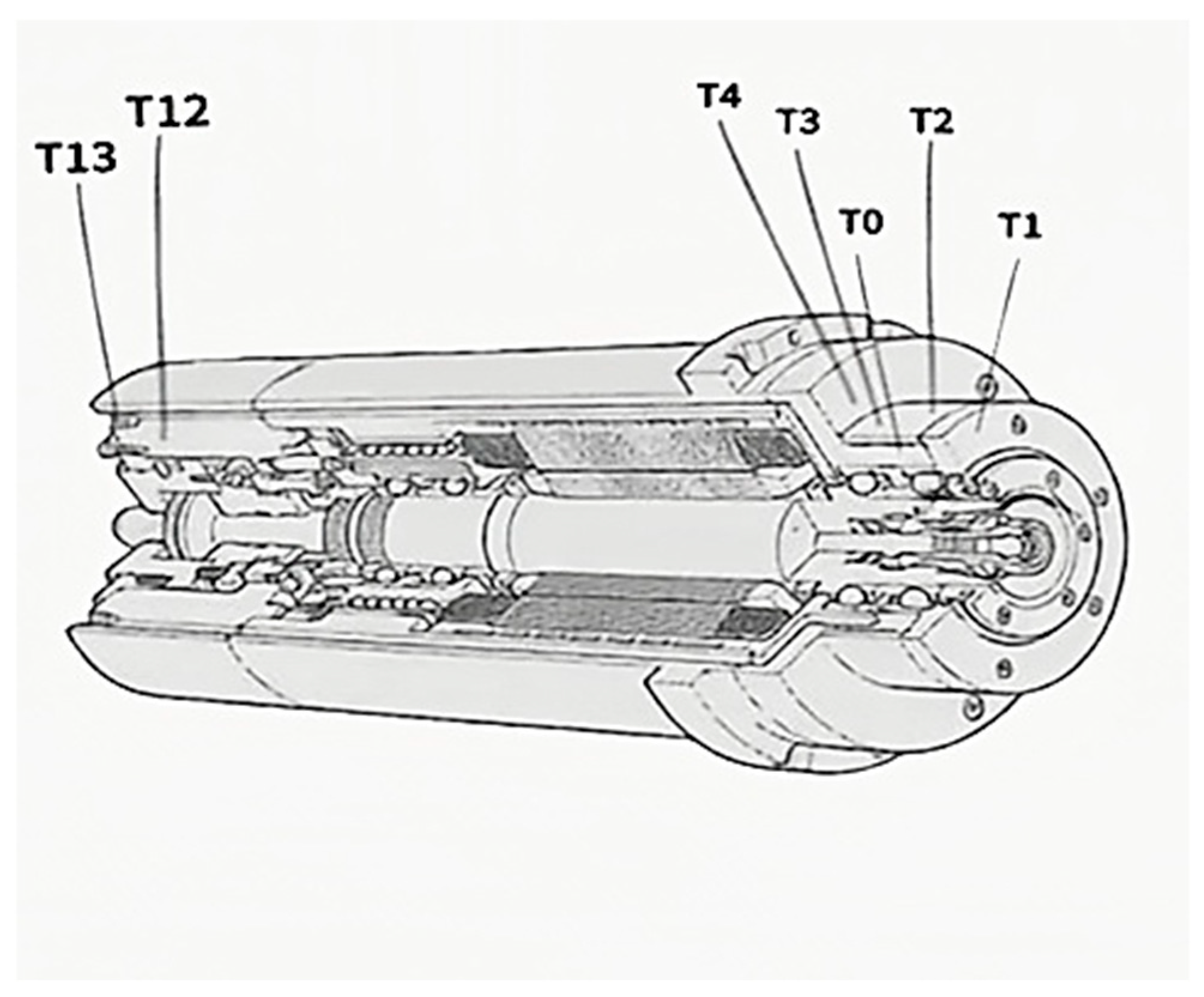
The design of the experimental setup and data acquisition process refers to the ISO 230-3 standard [54], which provides guidelines for evaluating the thermal characteristics of machine tools. The experimental dataset consists of multiple sets of temperature measurement data and corresponding spindle thermal error data collected from a CNC machine tool. Specifically, it includes 16 temperature sensors, seven of which are distributed along the central axis of the motorized spindle. The layout of the sensors is shown in Figure 5. The numbering and positioning of the sensors are described as follows:

T0 represents the temperature inside the front bearing, T1 denotes the temperature at the end face of the front bearing housing, T2 and T3 indicate the temperatures on both sides of the front bearing housing, T4 is the temperature on the outer surface of the front bearing, T12 represents the temperature inside the rear bearing, and T13 is the temperature outside the rear bearing. Additionally, the other seven temperature sensors are distributed at the water inlet and outlet of the front bearing, the water inlet and outlet of the motor, and the front, middle, and rear sections of the cooling jacket. Two more sensors measure the temperature of the worktable T14 and the surrounding environment T15.

For clarity and quick reference, the complete specifications of all temperature sensors are summarized in

Table 5. Summary of temperature sensor specifications.

Sensor ID	Location Description	Primary Measurement Objective
T0	Inside the front bearing	Core temperature of the primary heat source
T1	End face of the front bearing housing	Axial housing temperature
T2, T3	Two sides of the front bearing housing	Radial temperature gradient
T4	Outer surface of the front bearing	Bearing surface temperature
T5, T6	Inlet/Outlet, front bearing cooling	Cooling efficiency (ΔT) of front bearing circuit
T7, T8	Inlet/Outlet, motor cooling	Cooling efficiency (ΔT) of motor circuit
T9, T10, T11	Front, Middle, Rear of the cooling jacket	Spatial temperature distribution
T12	Inside the rear bearing	Core temperature of the rear bearing
T13	Outside the rear bearing	Rear bearing housing temperature
T14	Worktable	Structural reference temperature
T15	Ambient environment	Baseline ambient temperature

.

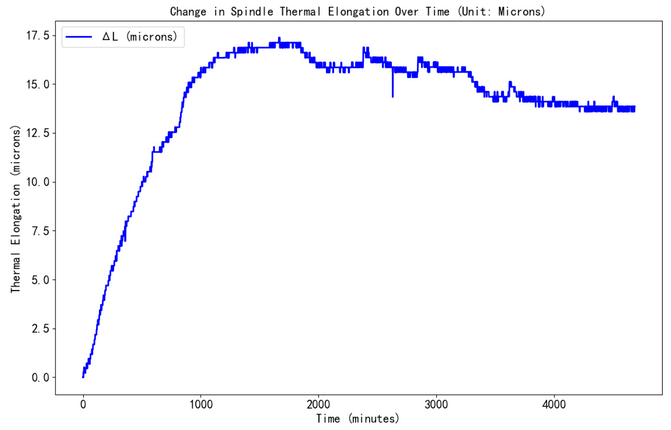
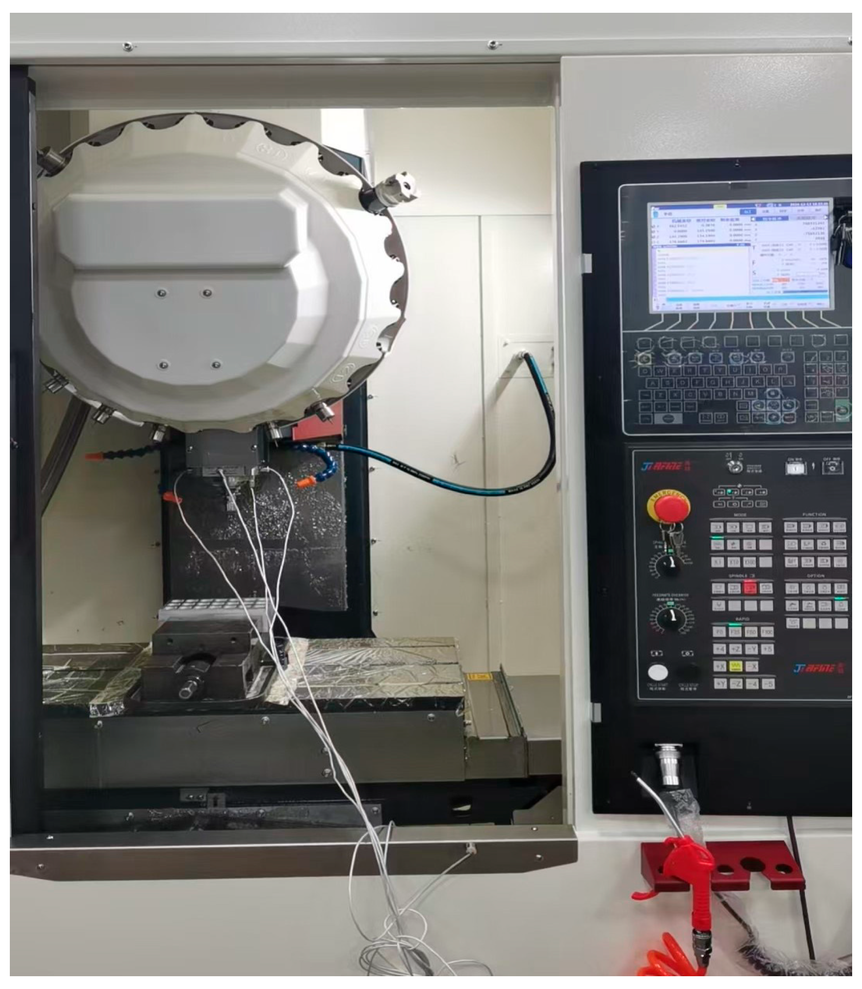
Thermal error data was measured using a laser displacement sensor to monitor the Z-direction displacement of the spindle end face in real time, with a sampling frequency of 1 Hz. Temperature and displacement data were synchronously collected through the machine tool system, forming a timestamp-aligned dataset.

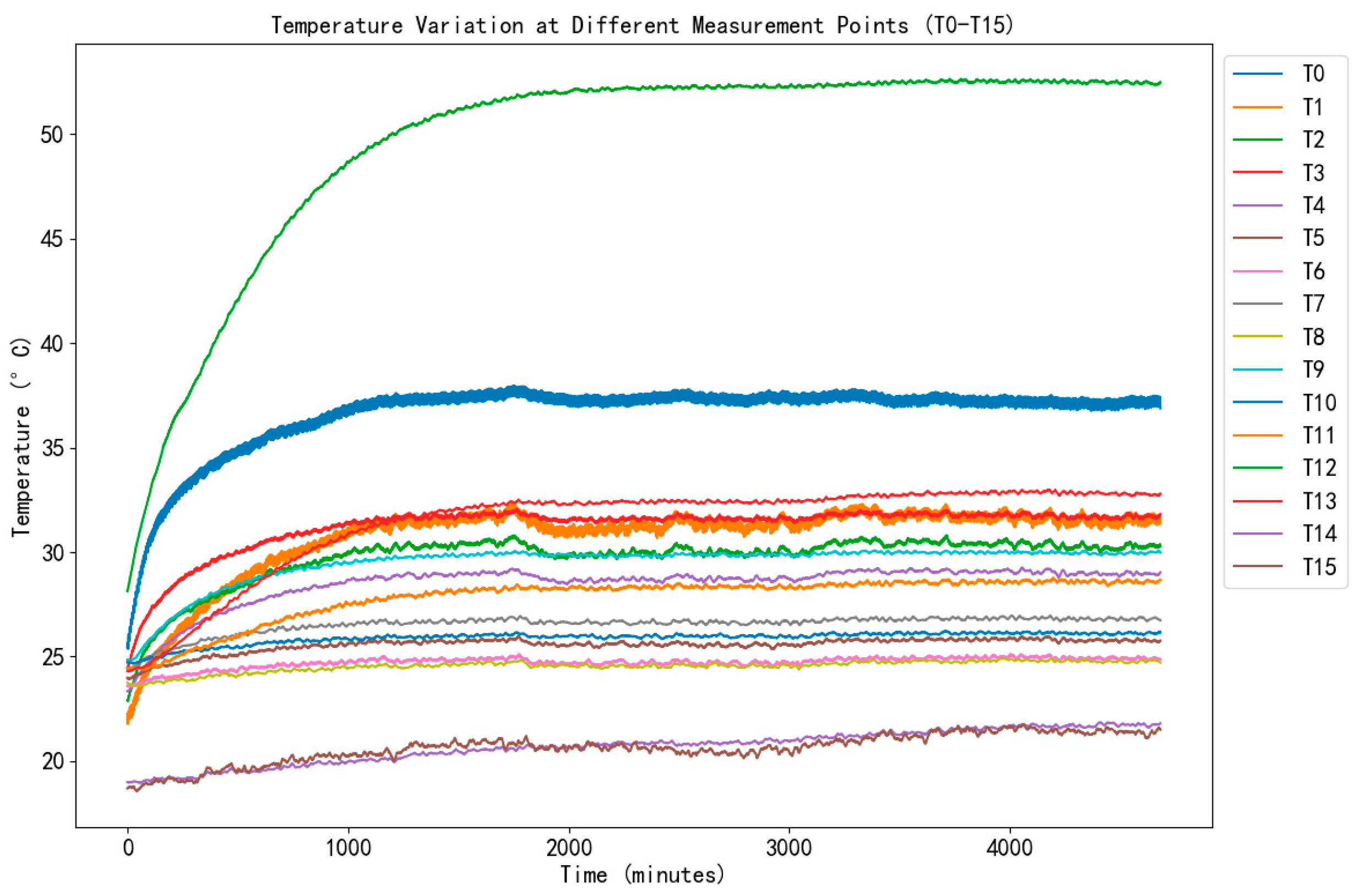
We collected 4682 sets of synchronised spindle thermal error and temperature data at one-minute intervals, capturing minute-wise error changes under different conditions. To ensure the consistency and applicability of the data, all data were normalized and randomly divided into training, validation, and test sets in an 8:1:1 ratio. Each temperature point reflects the temperature variation at different locations. The PSO-HDBSCAN algorithm is used to select the temperature points highly correlated with spindle thermal errors. These selected temperature points will be used as input features for the RBMO-X-DLTK model, for subsequent model training and prediction. The collected temperature data vary with the measurement time, as shown in Figure 6, and the spindle thermal error data change with the measurement time, as shown in Figure 7:

5.2. Analysis of Temperature Point Selection Effectiveness

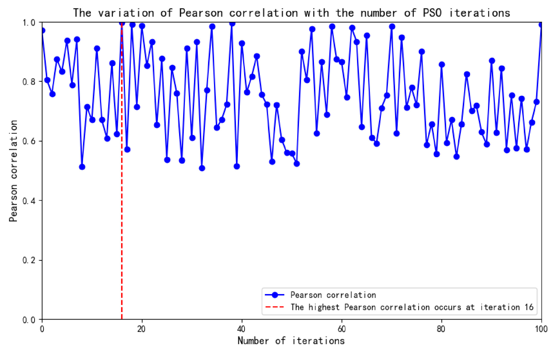
To verify the clustering performance of the PSO-HDBSCAN algorithm, the PSO optimization algorithm was first used to optimize the parameters based on the experimental setup. The Pearson correlation coefficient was calculated, and the optimal parameters were determined based on its magnitude. Figure 8 shows the trend of the Pearson correlation coefficient over 100 iterations.

In Figure 8, the highest Pearson correlation of 0.99697 occurs at the 16th iteration, with the optimized HDBSCAN algorithm parameters shown in

Table 6. Optimized HDBSCAN parameters.

Parameter	Value
Minimum Samples	5
Minimum Cluster Size	13
Density Propagation Parameter	0.8
Cluster Separation Precision	0.4

.

Using these optimized parameters, the HDBSCAN clustering algorithm can automatically identify clusters of varying densities and then evaluate the clustering results using metrics such as the Davies-Bouldin index, Silhouette Score, and BWP. The evaluation results are shown in

Table 7. Comparison of clustering performance.

Method	DB	Silhouette	BWP
HDBSCAN	1.98	0.71	2.081
PSO-HDBSCAN	1.72	0.94	3.104

.

The experimental results show that the DB index of the PSO-HDBSCAN algorithm decreased by 13.13%, the Silhouette index increased by 32.39%, and the BWP index increased by 49.16%, significantly outperforming the unoptimized HDBSCAN algorithm, indicating that the PSO-HDBSCAN algorithm significantly improves clustering performance.

To validate the effectiveness of the PSO-HDBSCAN optimization algorithm in selecting temperature points, clustering was first performed on the temperature points T0–T15 in the dataset, using Pearson, Spearman, and Kendall correlation coefficients to select the temperature clusters most correlated with thermal error. Based on the three metrics, the top three clusters most correlated with thermal error were selected through the above steps, as shown in

Table 8. Cluster Correlation.

Temperature Cluster	Pearson	Kendall	Spearman
Cluster 1	0.93656	0.94565	0.96128
Cluster 3	0.90645	0.93469	0.95327
Cluster 4	0.85103	0.92291	0.94259

.

The PSO-HDBSCAN algorithm was designed to converge to a stable solution. In our experiments, multiple runs with different initializations consistently identified the same optimal cluster (Cluster 1). The observed correlation coefficients for this cluster across runs showed negligible variation, confirming the high repeatability of the selection process. Therefore, based on the correlation coefficients in Table 8, the cluster with the highest overall correlation is selected as the optimal choice. Therefore, the temperature points in this cluster are considered the best thermal-sensitive points: the internal temperature of the front bearing (T0), the temperature at the end face of the front bearing housing (T1), the temperatures on both sides of the front bearing housing (T2 and T3), the temperature on the outer surface of the front bearing housing (T4), the temperature inside the rear bearing (T12), and the surrounding environment temperature (T15).

The inclusion of the ambient temperature (T15) in the optimal cluster is not merely a statistical correlation but is well supported by thermal dynamics. As a critical boundary condition, the ambient temperature directly influences the initial thermal state and heat dissipation efficiency of the entire machine tool structure. Changes in the ambient environment alter the thermal gradient between the spindle assembly and its surroundings, thereby modulating the system’s thermal equilibrium point and the dynamic response to internal heat sources. Consequently, T15 provides essential contextual information for predicting the spindle’s net thermal displacement under varying workshop conditions. Its selection by the PSO-HDBSCAN algorithm underscores that a robust thermal error model must account for this external thermal load to achieve high accuracy and generalizability across different operating environments. Next, RMSE, MSE, and MAE are used as performance metrics. The best thermal-sensitive points are used as input features for the model, and performance comparisons are made with models using seven randomly selected temperature points and all temperature points as features, with a training cycle of 100 epochs. For fairness, the unoptimized DLTK model ensures that the results are not influenced by hyperparameters. The experimental results are shown in

Table 9. Comparison of Temperature Point Selection Effectiveness.

Model	RMSE (μm)	MSE (μm)	MAE (μm)
DLTK (Random Seven Temperature Points)	0.301	0.091	0.228
DLTK (All Temperature Points)	0.271	0.073	0.208
DLTK (Best Sensitive Points)	0.205	0.042	0.161

.

As shown in Table 9, using the best sensitive points selected by the PSO-HDBSCAN clustering algorithm as input features significantly outperforms models using seven randomly selected temperature points and all temperature points. Specifically, compared to the randomly selected seven temperature points, RMSE decreased by 31.89%, MSE by 53.85%, and MAE by 29.39%. Compared to using all temperature points, RMSE decreased by 24.35%, MSE by 42.47%, and MAE by 22.6%. The results effectively demonstrate the validity of the temperature points selected by the PSO-HDBSCAN clustering algorithm, providing a more reliable basis for subsequent modeling and optimization.

5.3. Analysis of RBMO-X Optimization Effectiveness

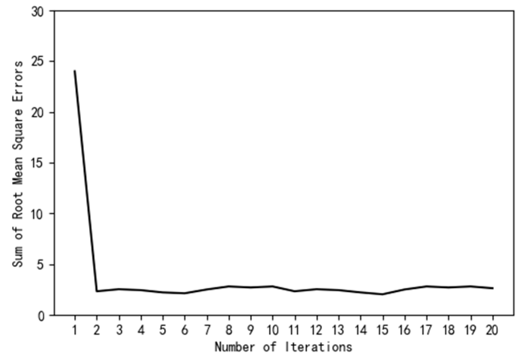
To validate the effectiveness of the hyperparameters optimized by the RBMO-X algorithm, hyperparameter tuning was performed based on the hyperparameter range defined in the experimental setup. The optimization effect was evaluated using the sum of the root mean square errors of spindle thermal errors, as shown in Figure 9.

It is evident from Figure 9 that the sum of the root mean square errors is minimized at the 15th iteration, indicating the lowest prediction loss. Therefore, the parameters from the 15th iteration are selected as the optimal parameters, as shown in

Table 10. Optimized DLTK Parameters.

Parameter	Value
Learning Rate	0.001
LSTM Hidden Layer Dimensions	64
Dropout Rate	0.1
Transformer Attention Heads	8
Fully Connected Layer Nodes	256
Batch Size	64
LSTM Layers	3
Loss Function	MAE

.

Using the best sensitive temperature points as input, the RBMO-X optimized DLTK model was used to predict spindle thermal errors. The model’s prediction performance was evaluated using metrics such as RMSE, MSE, MAE, R² Score, and EV Score. The model’s performance metrics are shown in

Table 11. Performance of RBMO-X-DLTK.

Model	RMSE	MSE	MAE	R2 Score	EV Score	VAF
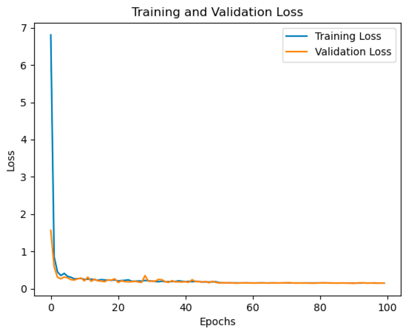
RBMO-X-DLTK	0.181	0.032	0.128	0.9978	0.9978	99.8%

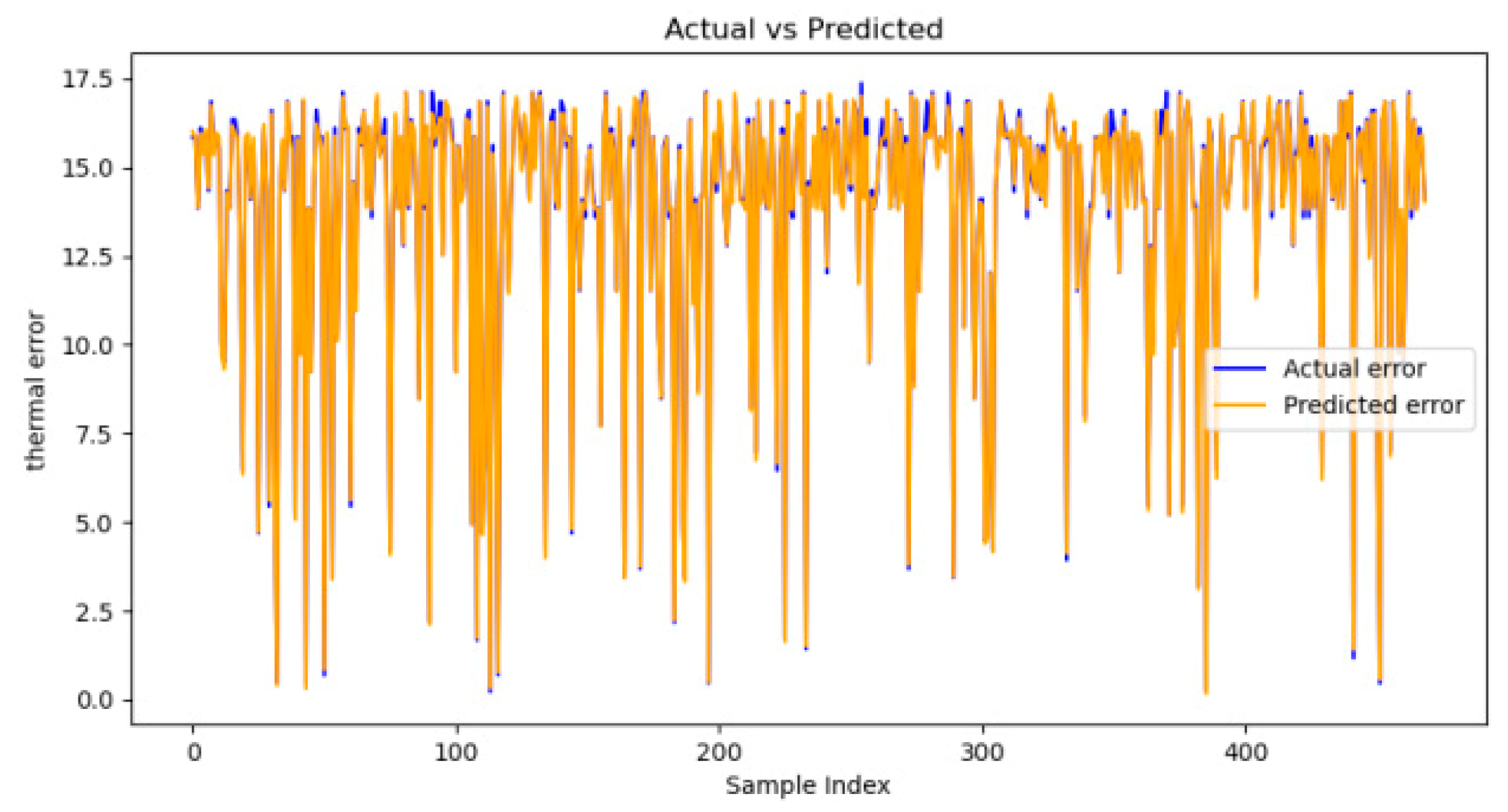
, with a training cycle of 100 epochs. The loss curve for each training iteration is shown in Figure 10, and the predicted errors from the RBMO-X-DLTK network model are compared with the actual values in Figure 11.

Figure 10 shows the change in training and validation loss over epochs. As the training epochs increase, both the training and validation losses decrease rapidly and stabilize, indicating continuous improvement and eventual convergence of the model’s performance on both the training and validation sets. Furthermore, the proximity of the training and validation loss curves suggests that the model does not suffer from overfitting or underfitting, demonstrating good generalization ability.

In Figure 11, the model’s predictive performance is visualized by comparing the actual error and prediction residuals. The figure shows that the difference between the actual error (blue) and the prediction error (orange) is small, and both display a consistent trend in most samples, indicating good prediction accuracy. The 98.83% prediction accuracy obtained in the experiment further demonstrates the model’s strong capability in predicting thermal errors.

The performance comparison between the optimized and unoptimized models is shown in

Table 12. Performance Comparison of DLTK and RBMO-X-DLTK.

Model	RMSE	MSE	MAE	R2 Score	EV Score	VAF
DLTK	0.205	0.042	0.161	0.9971	0.9974	99.7%
RBMO-X-DLTK	0.181	0.032	0.128	0.9978	0.9978	99.8%

:

These metrics show that the model optimized by the RBMO-X algorithm performs better across all key evaluation indicators. The improvement in RMSE and MAE, in particular, indicates that the optimized model not only reduces overall error but also enhances the model’s robustness and accuracy. This demonstrates the effectiveness of the RBMO-X algorithm in optimizing DLTK hyperparameters, allowing the model to better adapt to tasks such as spindle thermal error prediction in time-series forecasting.

5.4. Comparative Experiment

To validate the superiority of the RBMO-X-DLTK model, we compare it with seven established and state-of-the-art benchmark models for thermal error prediction: BP neural network [55], LSTM [56], and recent popular deep learning models such as the CNN-LSTM model and MA-CNN, the CNN-LSTM-Transformer model proposed by Al-Ali et al. [57] for solar power prediction, the TCN-LSTM hybrid model proposed by Li et al. [58] for predicting the health status and remaining useful life of lithium-ion batteries, and the SHO-LSTM model proposed by Chen et al. [59] for spindle thermal error modeling.

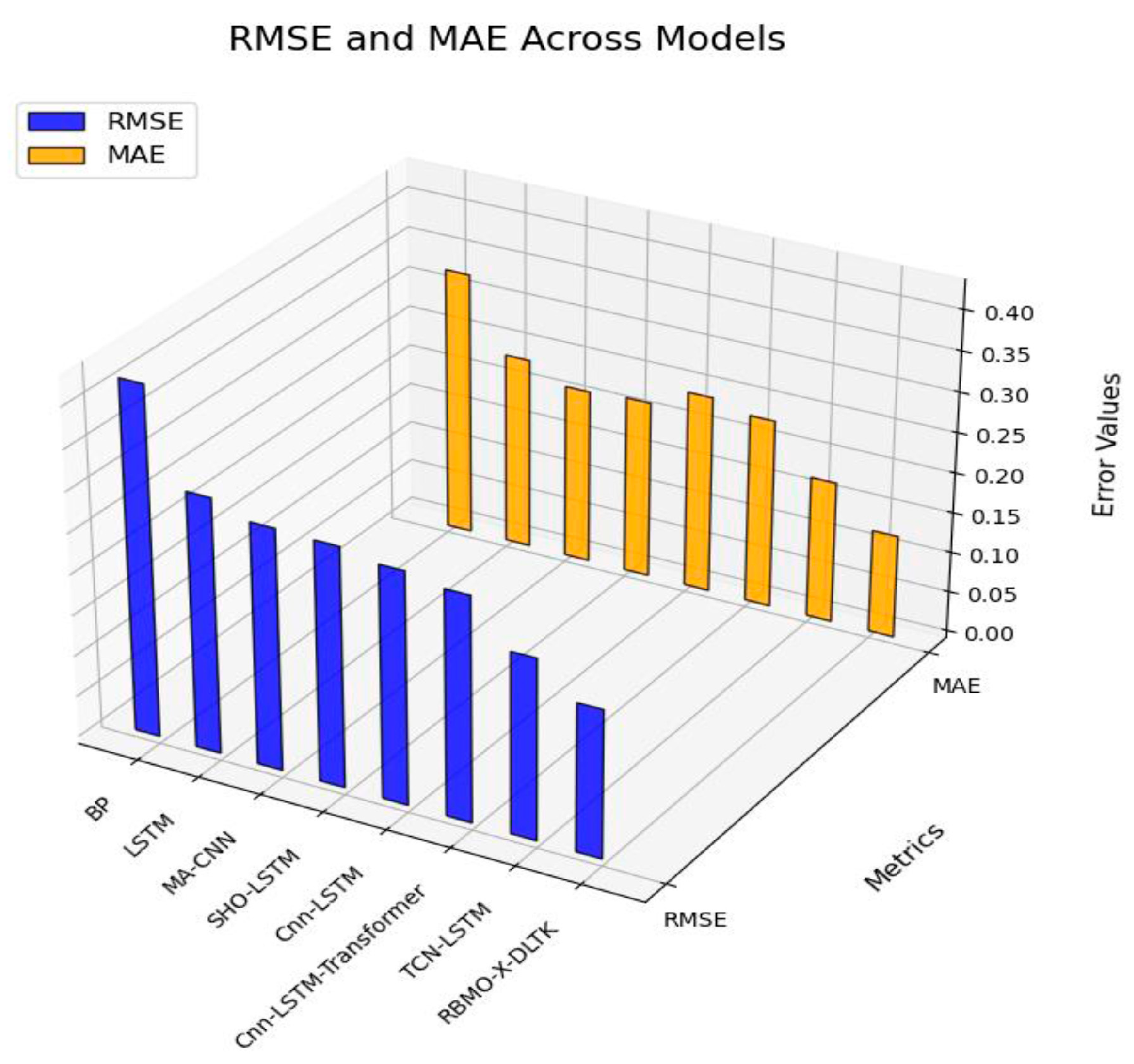
All models were trained and tested under identical conditions (same hardware, data split, input features, and 100 training epochs) to ensure a fair comparison. Their performance is comprehensively evaluated using RMSE, MAE, R², and other metrics, with results summarized in

Table 13. Comparison of Performance Metrics Across Models.

Model	RMSE	MSE	MAE	R2 Score	EV Score	VAF
BP	0.427	0.182	0.329	0.9866	0.9869	98.7%
LSTM	0.312	0.097	0.239	0.9934	0.9936	99.4%
MA-CNN	0.295	0.087	0.217	0.9941	0.9945	99.5%
SHO-LSTM	0.293	0.086	0.221	0.9942	0.9942	99.4%
CNN-LSTM	0.284	0.081	0.246	0.9945	0.9975	99.8%
CNN-LSTM-Transformer	0.275	0.076	0.235	0.9949	0.9976	99.8%
TCN-LSTM	0.221	0.049	0.176	0.9967	0.9977	99.8%
RBMO-X-DLTK	0.181	0.032	0.128	0.9978	0.9978	99.8%

and visually compared in Figure 12 and Figure 13.

As shown in Table 13, the RBMO-X-DLTK model achieves the lowest prediction error, with an RMSE of 0.181 and an MSE of 0.032. This represents a substantial improvement over all benchmarks. Specifically, it reduces RMSE by 57.6% compared to the BP model and by 42.0% compared to the LSTM model. Moreover, it maintains a clear advantage over recent advanced hybrids, achieving an 18.1% lower RMSE than TCN-LSTM and 34.2% lower than CNN-LSTM-Transformer. Similarly, the proposed model attains the lowest MAE of 0.128 μm, which is 61.1% and 46.4% lower than that of the BP and LSTM models, respectively. It also surpasses the best-performing baseline, TCN-LSTM (MAE = 0.176 μm), by a margin of 27.3%.

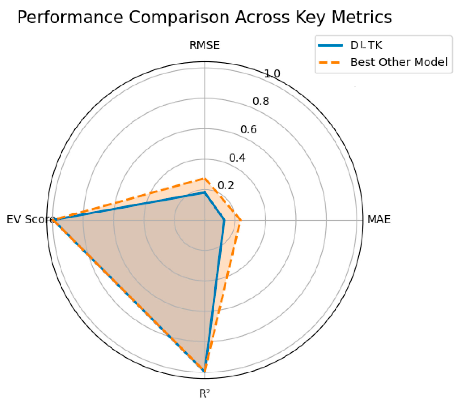
In terms of R² and EV Score, as shown in Figure 13, the DLTK model also performs exceptionally well, achieving values of 0.9978 for both, indicating its superior ability to explain data variance and capture the trend of thermal error changes. In comparison, the BP model has an R² of 0.9866 and an EV Score of 0.9869, while the LSTM model achieves 0.9934 and 0.9936, respectively, suggesting weaker explanatory power and generalization ability in these traditional models. Although the MA-CNN (R² = 0.9941, EV Score = 0.9945) and SHO-LSTM (R² = 0.9942, EV Score = 0.9942) models show some improvement in explaining thermal error, they still do not perform as well as DLTK. The CNN-LSTM-Transformer model and the TCN-LSTM model, which integrate LSTM and Transformer mechanisms, show slight improvements, with R² and EV Score reaching 0.9967 and 0.9977, respectively, demonstrating good explanatory power, but still fall short of DLTK. This hierarchy of model performance is consistently reflected in the Variance Accounted For (VAF) metric, with our RBMO-X-DLTK achieving the highest VAF score (see Table 13).

The validity of these comparative results is underscored by the deterministic experimental design. The substantial and consistent performance gains of RBMO-X-DLTK over all baseline models are observed under a tightly controlled framework (fixed data split and seeds). The large-margin superiority across every metric (e.g., >18% RMSE reduction versus the strongest baseline) provides compelling evidence that the improvement is inherent to the proposed methodology, not an artifact of random variation. In the context of architectural innovation, such conclusive empirical evidence establishes the practical efficacy of the framework.

Therefore, the experimental evidence confirms that the RBMO-X-DLTK framework establishes a new state-of-the-art for spindle thermal error prediction on the tested platform, significantly outperforming both traditional and state-of-the-art deep learning models.

Beyond prediction accuracy, computational efficiency is critical for industrial deployment.

Table 14. Computational efficiency and model complexity.

Model	Training Time (s)	Inference Time (ms/Sample)	Parameters (M)
BP	84.1	0.083	0.25
LSTM	103.6	0.096	0.74
MA-CNN	136.5	0.127	1.37
SHO-LSTM	127.6	0.119	1.23
CNN-LSTM	209.2	0.125	2.38
CNN-LSTM-Transformer	255.6	0.131	3.94
TCN-LSTM	130.4	0.116	1.25
RBMO-X-DLTK	116.9	0.114	1.31

benchmarks the training time, inference latency, and model complexity of all compared models under identical experimental conditions.

The results reveal two key insights for deployment:

(1)

Inference Efficiency: The inference latency of all deep learning models, including ours, is on the order of ~0.1 ms per sample. This is negligible compared to the thermal time constants of the spindle (minutes) and is fully compatible with the real-time control cycle of CNC systems.

(2)

Favorable Training Cost-Complexity Trade-off: While simpler models (BP, LSTM) have the lowest training times, the proposed RBMO-X-DLTK achieves significantly faster training (116.9 s) and lower complexity (1.31 M parameters) than other advanced hybrid architectures of comparable accuracy (e.g., CNN-LSTM, CNN-LSTM-Transformer). This demonstrates that the superior predictive accuracy of RBMO-X-DLTK (established in Table 13) is achieved with a competitive and often more efficient computational profile, striking a practical balance between performance and overhead for real-world deployment.

Comparison with Lightweight Models and Real-Time Deployment Considerations. It is noteworthy that our comparative study already includes two classic, lightweight models: the BP neural network and the LSTM network, which are widely adopted in embedded and real-time systems due to their structural simplicity and low computational demand. As shown in Table 13, while these models exhibit low inference latency (Table 14), their prediction errors are significantly higher than that of RBMO-X-DLTK. This indicates a clear trade-off between model complexity and accuracy. The proposed RBMO-X-DLTK model achieves state-of-the-art accuracy while maintaining an inference latency of 0.114 ms, which is orders of magnitude faster than the thermal dynamics of the spindle and thus fully compatible with real-time control cycles. Therefore, for high-precision thermal error compensation, the substantial accuracy gain afforded by RBMO-X-DLTK justifies its moderately increased complexity, as the real-time constraint is unequivocally met.

5.5. Ablation Study

To further validate the effectiveness of each module in the proposed RBMO-X-DLTK model, a series of ablation experiments were designed, systematically removing key modules to observe their impact on overall performance. The ablation models include:

(1)

LSTM-Transformer-KAN: Removes the 1D-DC module, using only the LSTM, Transformer, and Fourier KAN modules.

(2)

1D-DC-Transformer-KAN: Removes the LSTM module, retaining only the 1D-DC, Transformer, and Fourier KAN modules.

(3)

1D-DC-LSTM-KAN: Removes the Transformer module, retaining only the 1D-DC, LSTM, and Fourier KAN modules.

(4)

1D-DC-LSTM-Transformer: Removes the Fourier KAN module, retaining only the 1D-DC, LSTM, and Transformer modules.

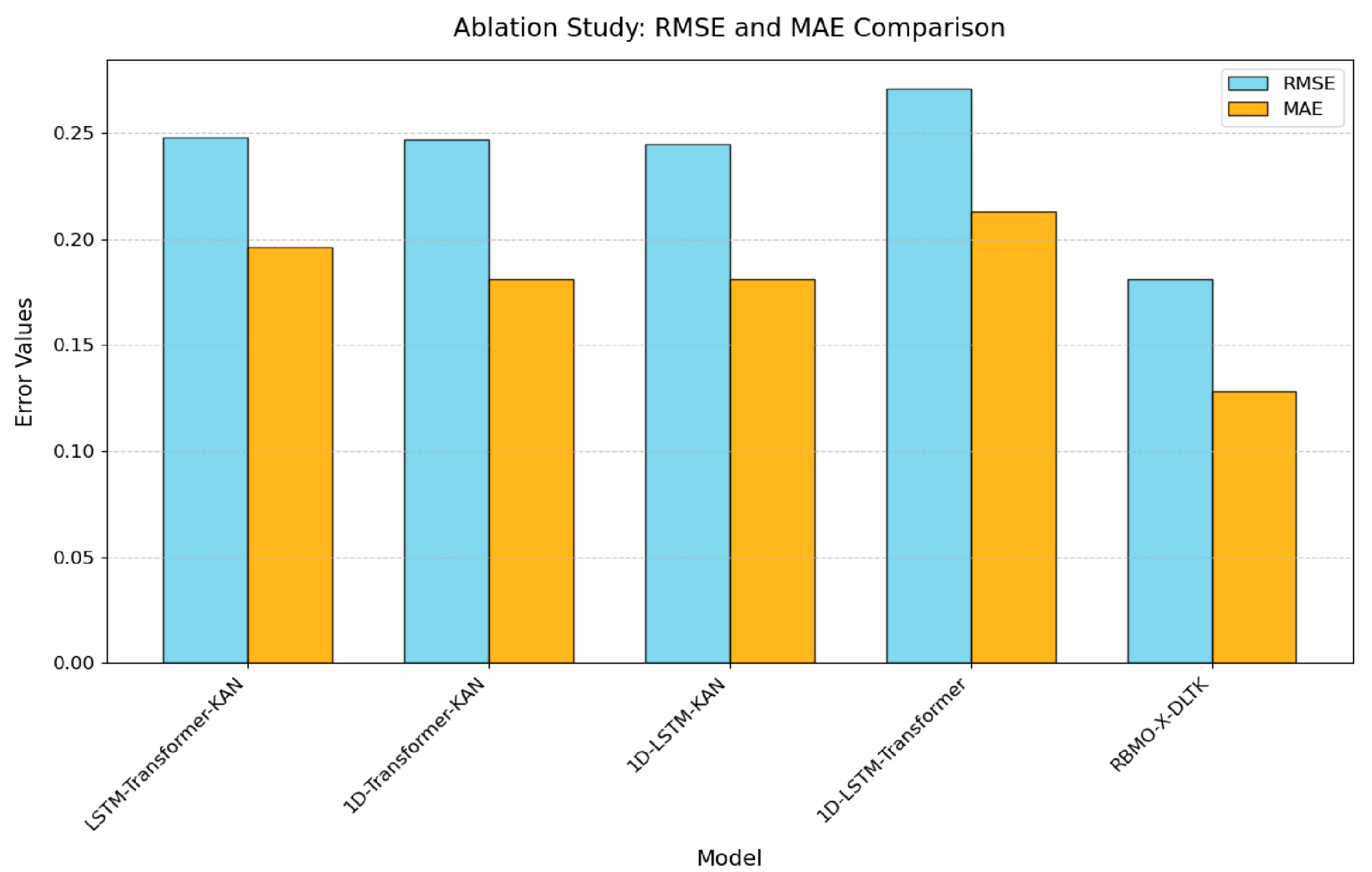
These ablation models are used to assess the contribution of each module to the overall model performance. The experimental setup is consistent with the main experiment, with the same dataset split, training, and testing conditions applied to all ablation experiments. The experimental results are shown in

Table 15. Ablation Experiment Performance Comparison.

Model	RMSE	MSE	MAE	R2 Score	EV Score	VAF
LSTM-Transformer-KAN	0.248	0.062	0.196	0.9958	0.9961	99.6%
1D-DC-Transformer-KAN	0.247	0.061	0.181	0.9958	0.9960	99.6%
1D-DC-LSTM-KAN	0.245	0.060	0.181	0.9959	0.9959	99.6%
1D-DC -LSTM-Transformer	0.271	0.073	0.213	0.9950	0.9955	99.5%
RBMO-X-DLTK	0.181	0.032	0.128	0.9978	0.9978	99.8%

and Figure 14.

As shown in Table 15 and Figure 14, the complete DLTK model outperforms all other configurations across all metrics, particularly achieving RMSE and MAE values of 0.181 and 0.128, respectively, which are significantly better than any ablation experiment. The ablation study further demonstrates that the model’s predictive performance relies on the synergy of all modules, with the removal of any module leading to a marked decline in performance.

As shown in Table 9 and Table 15, the model without the 1D-DC module (LSTM-Transformer-KAN) exhibits higher RMSE (0.248) and MAE (0.196), significantly worse than the models that include this module. This indicates that 1D-DC plays a crucial role in feature extraction and capturing local variations. Moreover, compared to the CNN-LSTM combination, the inclusion of 1D-DC better adapts to the nonlinear characteristics of the machine tool temperature signals, significantly enhancing feature extraction capability and model robustness. The experimental results validate the importance of this module in improving prediction accuracy.

The model without the Fourier KAN module performs worse in all error metrics compared to those with it. For instance, the 1D-LSTM-Transformer model without Fourier KAN has an RMSE of 0.271 and MAE of 0.213, significantly higher than the 1D-Transformer-KAN and 1D-LSTM-KAN models with Fourier KAN (RMSE of 0.245–0.247, MAE of 0.181). This indicates that the Fourier KAN module plays a crucial role in extracting and analyzing frequency-domain features, which improves the model’s thermal error prediction accuracy. Specifically, in reducing RMSE and MAE, the Fourier KAN module effectively reduces prediction errors and enhances the overall performance of the model. Therefore, the ablation experiment results confirm the importance of the Fourier KAN module in enhancing the model’s prediction accuracy and robustness.

Removing either the LSTM module or the Transformer encoder leads to a decrease in performance, but the impact is less significant than removing the Fourier KAN module. This indicates that the LSTM and Transformer modules play crucial roles in modeling temporal dependencies and extracting global features, respectively, and their combined effect further improves the prediction accuracy.

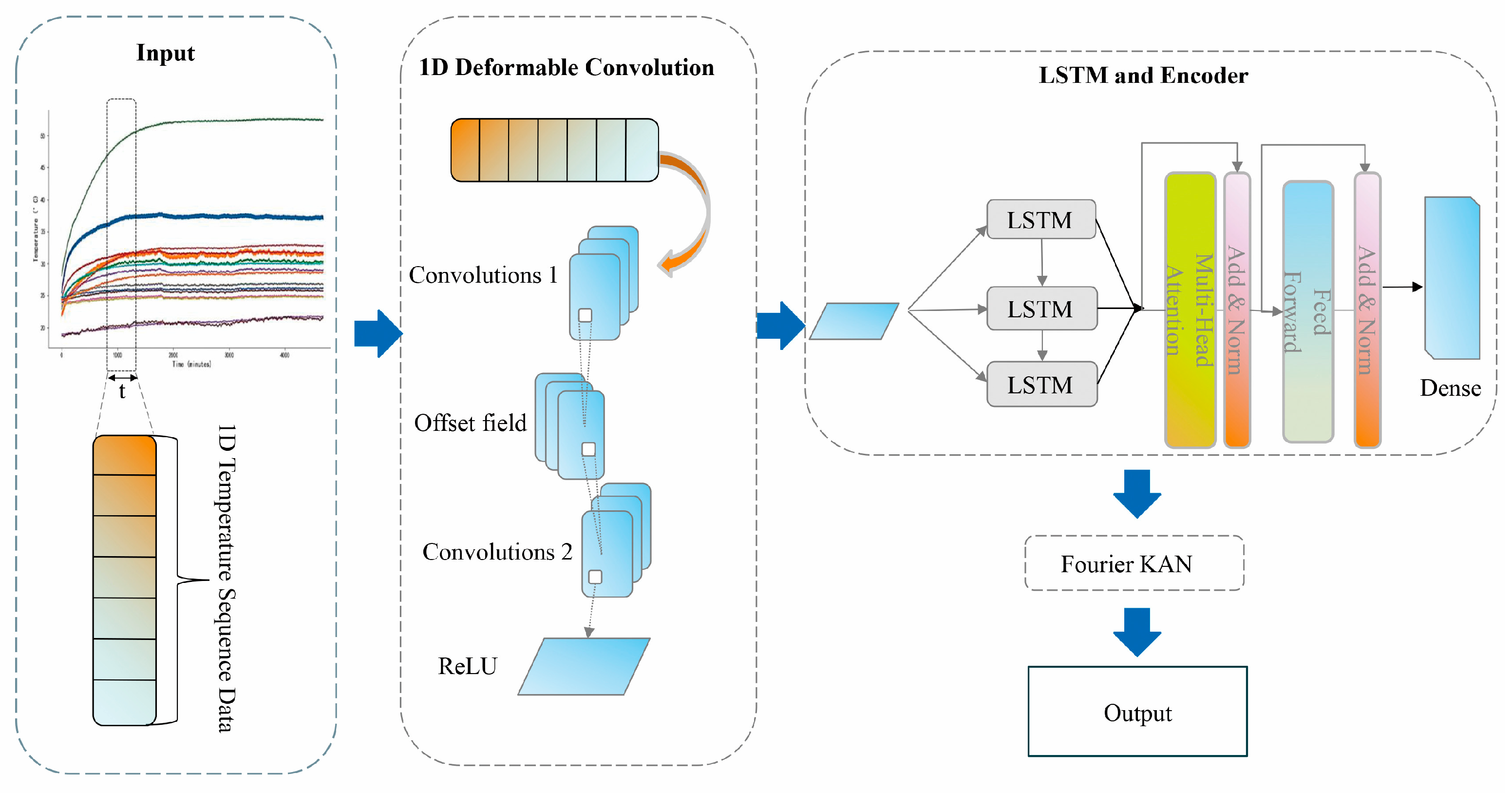
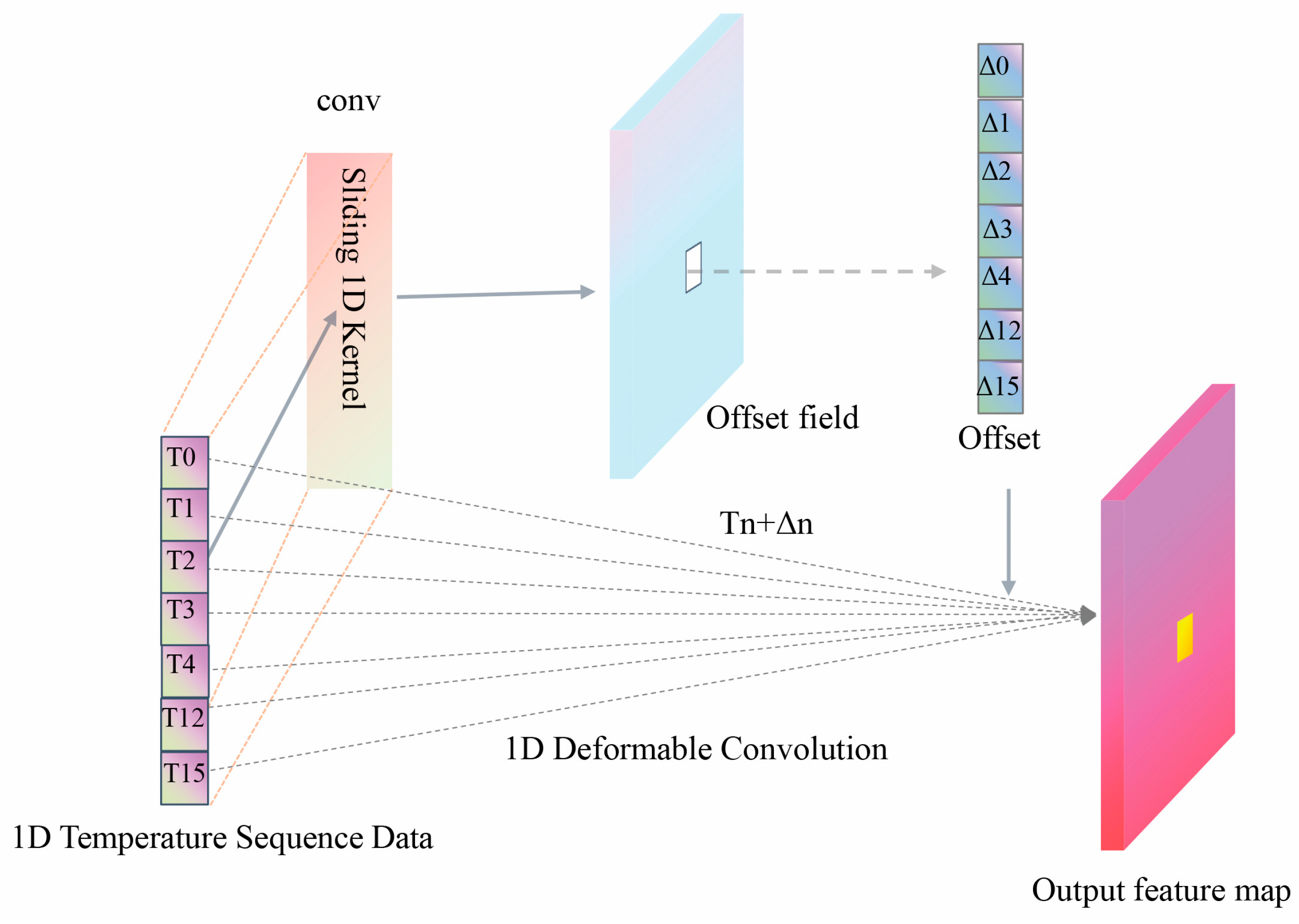
Overall, the complete DLTK model performs best in key metrics such as RMSE and MAE. Removing any of the LSTM, Transformer, or Fourier KAN modules leads to a significant decline in model performance. The experimental results further demonstrate that the collaboration of the 1D deformable convolution, LSTM, Transformer, and Fourier KAN modules is crucial for enhancing feature extraction capabilities and prediction accuracy. The 1D deformable convolution enhances local feature extraction, LSTM captures long-term dependencies in the time series, the Transformer explores global features through the self-attention mechanism, and the Fourier KAN module improves prediction accuracy and stability through frequency domain analysis.

5.6. Evaluation Metrics

The root mean square error (RMSE) and mean absolute error (MAE) are employed as primary metrics because they provide interpretable, scale-dependent measures of the average prediction error in micrometers (μm), which directly relates to the magnitude of thermal displacement critical for machining accuracy [60,61]. RMSE penalizes larger errors more heavily, making it sensitive to undesirable large deviations, while MAE offers a robust measure of average error magnitude. The coefficient of determination (R²), explained variance score (EV Score) and the variance accounted for (VAF) complement these by quantifying the proportion of variance in the thermal error that is captured by the model, thus assessing its overall fitting capability. While application-specific error thresholds (e.g., a maximum allowable thermal error) are ultimately crucial for acceptance, these standard metrics provide a comprehensive, granular, and widely comparable assessment of model performance across its entire operating range, forming the necessary foundation for evaluating whether a model can meet such thresholds.

Accordingly, in this study, the evaluation framework comprises two categories of metrics: the first measures clustering effectiveness for temperature point selection, and the second evaluates the regression performance of the thermal error prediction models. The specific metrics are defined as follows:

Pearson correlation is used to assess the linear correlation between two variables, with values closer to ±1 indicating a stronger correlation. Kendall and Spearman are used to evaluate the nonlinear correlation between two variables, with values ranging from [−1, 1], as shown in Equations (7)–(9).

$$r={\displaystyle \frac{\sum \left(x_i-\overline{x}\right)\left(y_i-\overline{y}\right)}{\sqrt{\sum {\left(x_i-\overline{x}\right)}^2\sum {\left(y_i-\overline{y}\right)}^2}}}$$

(7)

$$K={\displaystyle \frac{\left(C-D\right)}{\frac{1}{2}n\left(n-1\right)}}$$

(8)

$$\rho =1-{\displaystyle \frac{6\sum d_i^2}{n\left(n^2-1\right)}}$$

(9)

where $x_i$ and $y_i$ represent the observed values of two variables, while $\overline{x}$ and $\overline{y}$ are the mean values of $x$ and $y$ respectively. $r$ is the Pearson correlation coefficient, which ranges from −1 to 1. $K$ is the Kendall index, where $C$ is the number of concordant pairs, $D$ is the number of discordant pairs, and $n$ is the total number of temperature points. $\rho$ is the Spearman index, and $d_i$ represents the rank difference.

Davies-Bouldin, Silhouette, and BWP are metrics used to evaluate clustering performance. The lower the DB value, the better the clustering result. The Silhouette score ranges from −1 to 1, with higher values indicating better clustering. A higher BWP value indicates better separation between clusters and greater cohesion within clusters. The formulas are shown in Equations (10)–(14).

$$DB={\displaystyle \frac{1}{N}}\sum _{i=1}^N \underset{j\ne i}{max} \left({\displaystyle \frac{s_i+s_j}{d_{i,j}}}\right)$$

(10)

$$s\left(i\right)={\displaystyle \frac{b\left(i\right)-a\left(i\right)}{\mathit{max}\left(a\left(i\right),b\left(i\right)\right)}}$$

(11)

$$BWP={\displaystyle \frac{SSB}{SSW}}$$

(12)

$$SSB=\sum _{i=1}^N \sum _{j=1}^N \parallel c_i-c_j{\parallel }^2$$

(13)

$$SSW=\sum _{i=1}^N \sum _{x\in C_i} \parallel x-c_i{\parallel }^2$$

(14)

where $N$ represents the number of clusters, $s_i$ and $s_j$ indicate the intra-cluster average distance of clusters $i$ and $j$, and $d_{i,j}$ is the distance between clusters $i$ and $j$. $s_i$ is the Silhouette score, where $a\left(i\right)$ is the average distance from sample $i$ to other samples in its cluster, and $b\left(i\right)$ is the average distance from sample $i$ to the nearest cluster. $SSB$ is the sum of squares between clusters (the squared distance between cluster centroids), where $c_i$ and $c_j$ are the centroids of clusters $i$ and $j$, and $SSW$ is the sum of squares within clusters (the squared distance between points and the centroid within each cluster), with $x$ representing the sample points in cluster $i$.

Root Mean Squared Error (RMSE), Mean Squared Error (MSE), Mean Absolute Error (MAE), R² Score (Coefficient of Determination), and Explained Variance Score (EV Score) are commonly used to assess the performance of regression models. The smaller the RMSE, MSE, and MAE, and the higher the R² Score and EV Score (closer to 1), and VAF (closer to 100%), the higher the model’s prediction accuracy. The formulas are shown in Equations (15)–(20).

$$RMSE=\sqrt{{\displaystyle \frac{1}{n}}\sum _{i=1}^n (y_i-{\hat{y}}_i{)}^2}$$

(15)

$$MSE={\displaystyle \frac{1}{n}}\sum _{i=1}^n (y_i-{\hat{y}}_i{)}^2$$

(16)

$$MAE={\displaystyle \frac{1}{n}}\sum _{i=1}^n \left|y_i-{\widehat{y}}_i\right|$$

(17)

$$R^2=1-{\displaystyle \frac{\sum (y_i-{\widehat{y}}_i{)}^2}{\sum (y_i-\overline{y}{)}^2}}$$

(18)

$$EV=1-{\displaystyle \frac{Var\left(y-\widehat{y}\right)}{Var\left(y\right)}}$$

(19)

$$EV=[1-{\displaystyle \frac{Var\left(y-\widehat{y}\right)}{Var\left(y\right)}}]\times 100\%$$

(20)

where $y_i$ represents the true values, ${\widehat{y}}_i$ represents the predicted values, $n$ is the number of samples, $\overline{y}$ is the mean of the true values, and $Var\left(y\right)$ is the variance of $y$.

6. Real-Machine Compensation Validation

To verify the prediction accuracy and compensation capability of the RBMO-X-DLTK model for spindle thermal errors in practical industrial applications, a series of machining experiments were designed. The experiments used the T-5C and T-7C CNC machines from Qiaofeng [62] as experimental equipment, as shown in Figure 15. The experiments were divided into uncompensated and compensated testing, according to the practical requirements for machine tool thermal error compensation. In the uncompensated tests, workpieces were machined separately, and the thermal error variation curve for each machining operation was recorded. The maximum thermal elongation was measured within 1 h after machine startup, and the stable error value after continuous machining was recorded. The compensated tests included real-time prediction and compensation of thermal errors based on the RBMO-X-DLTK model, and the change in dimensional accuracy after compensation was recorded.

Tests occurred in a temperature-controlled environment (28 °C) to eliminate external thermal interference. The workpiece surfaces were kept level, and the top and side surfaces of the workpieces were aligned. A total of two workpieces were processed, each consisting of 21 parts. Each part contains a large rounded rectangular hole and a small runway circular hole, forming two steps. In the experiment, the depth of the rounded rectangular holes was 5 mm and the depth of the runway circular holes was 7 mm (symmetrical on all four sides, with the top surface as the reference plane, and the top and side surfaces of the two workpieces aligned). Machining followed the sequence shown in Figure 16, steps 1–42. Roughing and finishing speeds were set to 7000 r/min, with rough feed rates of 3000 mm/min for the rounded rectangular holes and 2500 mm/min for the runway circular holes. Finishing feed rates were set to 600 mm/min. The three-coordinate measurement was used with the top surface as the reference plane (zero plane) to measure the step heights. The heights of the steps labeled as 1 were used as the initial thermal elongation values, and the thermal elongation changes and steady-state values in the Z-direction were recorded. The experiment aimed to verify the model’s effect on improving machining accuracy and evaluate its stability and robustness under multiple operating conditions.

Verification Results

As shown in Figure 17 and Figure 18, after the machine tool has been idle for 1 h, the maximum Z-axis thermal expansion for the 5 mm workpiece is 0.0438 mm, and for the 7 mm workpiece, it is 0.0488 mm. The thermal error increases rapidly in the initial stage after machine startup but gradually stabilizes, indicating that the machine tool is approaching a steady state during the thermal stabilization process. However, this level of thermal error still has a significant impact on high-precision machining. After applying real-time compensation using the RBMO-X-DLTK model, the thermal error is significantly reduced. During continuous machining, the thermal error for the 5 mm workpiece stabilizes around 0.003 mm, while for the 7 mm workpiece, it decreases and stabilizes around 0.0024 mm. The average compensation rate reached 89%. The model accurately predicted the thermal error variation during 1 h of machining, effectively improving machining accuracy. Under continuous machining conditions, after compensation by the model, the Z-axis thermal error fluctuations stabilized. From machine startup to the stabilization of the machining state, although some over-compensation occurred, the overall compensation effect remained stable. This indicates that the RBMO-X-DLTK model has good robustness and generalization ability under complex conditions and can effectively handle thermal error variations under different machining conditions.

The above real-world validation successfully demonstrates the compensation effectiveness of the RBMO-X-DLTK model for the specified step-feature geometry under the tested machining conditions. Its generalization to a significantly broader spectrum of workpiece geometries (e.g., free-form surfaces, thin-walled parts) and more extreme machining operations (e.g., high-interruption cutting, different material types) requires further investigation, which is outlined as future work. Furthermore, the validation in this study is conducted on specific machine models (T-5C and T-7C). Generalizing the framework to different machine tools or spindle configurations would involve re-applying the proposed PSO-HDBSCAN methodology to identify temperature-sensitive points and may require model re-tuning based on the new thermal characteristics, which also constitutes an important direction for future validation and application.

7. Discussion

The experimental results show that the RBMO-X-DLTK model achieves a comprehensive improvement in prediction error and fit indicators compared to other models. This performance enhancement is largely attributed to the advantages of the PSO-HDBSCAN algorithm in selecting temperature points. PSO-HDBSCAN significantly reduces the redundancy of input features and ensures that the selected temperature points achieve optimal correlation with thermal errors. Compared to randomly selecting 7 temperature points or using all temperature points, the selected temperature points as input features reduced RMSE by 31.89%, MSE by 53.85%, and MAE by 29.39%. However, PSO-HDBSCAN still faces challenges in real-time applications, such as the potential impact on the algorithm’s iteration efficiency in high-dimensional feature scenarios. Moreover, the clustering parameter optimization required by this method may need further adjustment under dynamic working conditions to adapt to more complex thermal environments. In the future, it may be considered to introduce an adaptive parameter adjustment mechanism to further enhance the algorithm’s generalization ability under various operating conditions.

Beyond these algorithmic considerations, the framework’s robustness to imperfections in the input data itself—such as sensor noise or intermittent missing values—is another critical aspect for practical deployment. It is noteworthy that the PSO-HDBSCAN feature selection stage offers inherent resilience against sporadic, uncorrelated noise by design, as the HDBSCAN algorithm filters out points identified as outliers. This addresses a common class of data quality issues. For sustained systematic noise or extended data loss, which could impact the cluster structure, the integration of complementary signal processing or imputation techniques would be necessary. Enhancing robustness under these challenging data conditions is a clear direction for future work aimed at industrial hardening.

Interpretability and Physical Insights. Our framework directly addresses model interpretability through its PSO-HDBSCAN feature selection stage, which acts as a data-driven sensor importance analyzer. By consistently identifying the optimal temperature cluster (e.g., front/rear bearings and ambient temperature, as detailed in Section 5.2), it provides clear, physically grounded insight into the primary thermal influences on spindle error. This offers actionable guidance beyond mere black-box prediction, effectively bridging data-driven modeling with practical thermal management understanding.

Compared to DLTK, the RBMO-X-DLTK model reduces the overall error by about 13%, and this improvement is mainly attributed to the significant advantages of the RBMO-X algorithm in hyperparameter optimization. By combining SGDR and gradient clipping, RBMO-X significantly improves the model’s convergence speed and stability. Specifically, SGDR dynamically adjusts the learning rate, effectively avoiding getting stuck in local optima during training, allowing the model to better fit high-dimensional and complex feature data. On the other hand, gradient clipping limits the L2 norm of the gradient, eliminating the risk of gradient explosion and ensuring the stability of the DLTK model in multi-level feature extraction. In addition, RBMO-X’s collaborative global and local search mechanism enables hyperparameter optimization to quickly find the best configuration suited for complex working conditions. Although RBMO-X performs excellently in hyperparameter optimization, there is still a certain computational overhead in high-dimensional and complex feature scenarios. In the future, distributed optimization techniques could be combined to further improve its efficiency in large-scale data, and RBMO-X’s response speed for parameter adjustment under real-time dynamic conditions also has room for further optimization.

To substantiate the choice of the PSO algorithm for optimizing HDBSCAN parameters, a direct comparison with two other prevalent metaheuristic optimizers—the Grey Wolf Optimizer (GWO) [63] and the Firefly Algorithm (FA) [64]—was conducted. The comparison utilized the identical experimental setup: the same HDBSCAN parameter search bounds (Table 3), population size (20), maximum iterations (100), and objective function (maximizing the Pearson correlation between temperature clusters and thermal error). Standard parameter settings from the literature were used for GWO and FA to ensure a fair comparison. The performance metrics, summarized in

Table 16. Performance comparison of PSO with other optimizers for HDBSCAN parameter tuning.

Optimizer	Best Pearson Correlation	Iteration of Best Solution
Firefly Algorithm (FA)	0.98215	41
Grey Wolf Optimizer (GWO)	0.98742	34
PSO (Proposed)	0.99697	16

Note: All algorithms were run for a maximum of 100 iterations. The “Iteration of Best Solution” indicates the iteration at which the highest fitness value was first attained and remained unchanged.

, clearly demonstrate the advantage of PSO for this specific continuous parameter optimization problem. PSO not only achieved the highest Pearson correlation (0.99697) but also converged to this optimal solution in the fewest iterations (16). This empirical result validates the theoretical rationale provided in Section 3, confirming that PSO offers superior efficiency and convergence reliability in tuning HDBSCAN, thereby enhancing the robustness of the feature selection stage.

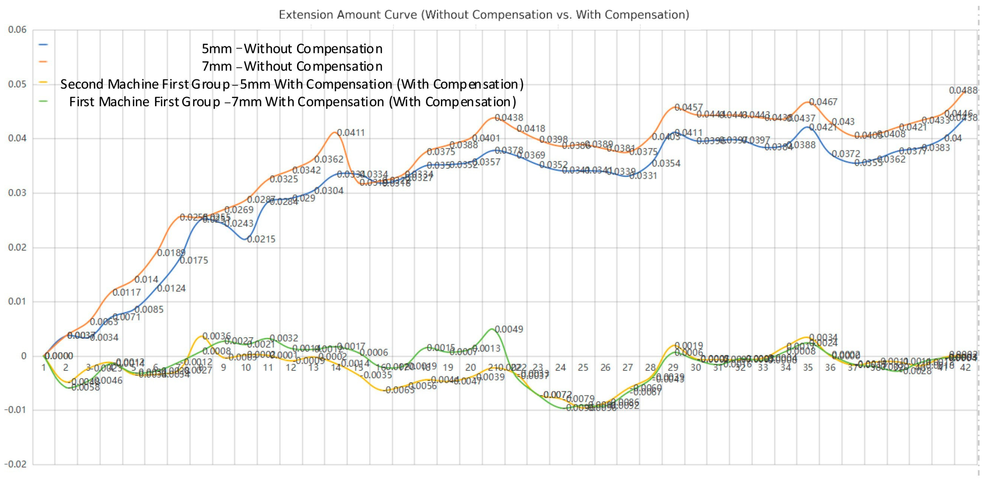
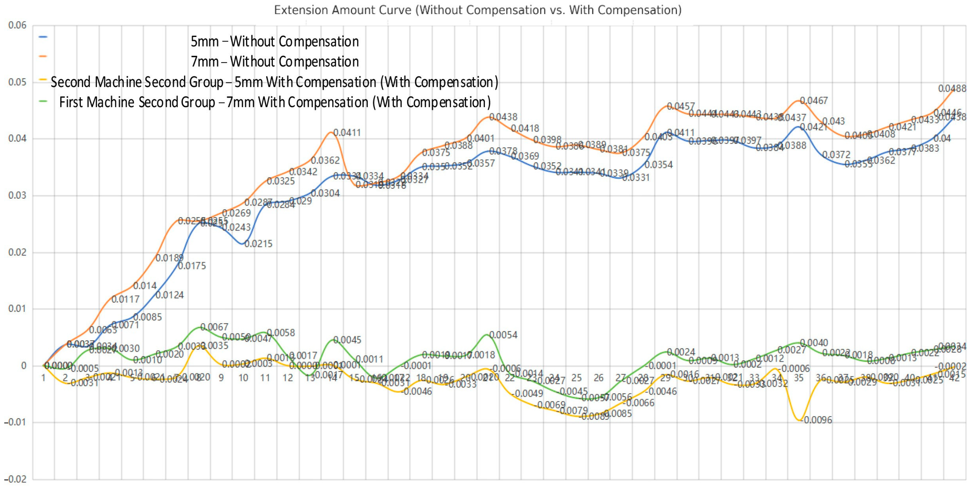
The observed discrepancy between the high prediction accuracy (98.83%) and the realized compensation rate (89%) underscores the transition from a data-driven predictive model to a physical compensation system. This gap can be attributed to several intertwined practical and dynamic limitations inherent in real-time machining environments:

(1)

Dynamic Response Lag of the Physical System: The RBMO-X-DLTK model predicts thermal error based on temperature history. However, the actual compensation system—comprising the CNC controller, servo drives, and mechanical axes—has inherent response delays (e.g., servo response time, communication latency). This finite response speed means the compensation command is always applied to a system state that is slightly ahead of the state on which the prediction was based, especially during periods of rapid thermal change.

(2)

Nonlinearities and Hysteresis in the Actuation Chain: The model assumes a perfect mapping from predicted error to compensated axis movement. In reality, the ball screw, guideways, and bearings exhibit nonlinear friction, backlash, and hysteresis. These effects introduce small, uncompensated errors between the command position and the actual tool tip position, which are not captured by the purely thermal-error-focused prediction model.

(3)

Unmodeled External Disturbances: The experimental validation involved actual cutting operations. Dynamic cutting forces, vibrations, and coolant effects introduce additional, non-thermal mechanical deformations that perturb the spindle position. Our model, trained primarily on thermally induced errors under idle or warm-up conditions, does not account for these coupled thermo-mechanical effects, leading to a predictable performance gap during real machining.

(4)

Synchronization and Sampling Limitations: While temperature and error data were synchronized during model training, the real-time compensation loop operates under strict sampling and execution cycles. Any jitter or minor asynchrony between temperature acquisition, model inference, and compensation command issuance can result in sub-optimal correction.

These factors collectively explain why a portion of the predicted error cannot be perfectly canceled in practice. The achieved 89% compensation rate, therefore, reflects the practically attainable performance of the integrated “sensor-model-controller” system, demonstrating significant improvement over the uncompensated case while highlighting areas for future work in co-modeling and adaptive control.

Given the complexity of the DLTK architecture, proactive measures were taken to ensure generalization and mitigate overfitting. First, architectural regularization was implemented through Dropout layers (with the rate optimized by RBMO-X, see Table 10). Second, and most critically, the model’s generalization capability is empirically validated by our rigorous evaluation protocol:

(1)

The 8:1:1 train/validation/test split ensured an unbiased assessment.

(2)

The close alignment between training and validation loss curves (Figure 10) indicates no significant overfitting during training;

(3)

Most importantly, the model maintained superior performance on the completely held-out test set (Table 13), demonstrating its ability to generalize to unseen data.

Finally, its successful application in the real-world machining validation (Section 6), a distinctly different environment, provides strong external evidence of its robustness beyond the original dataset.

Beyond the internal technical validation and comparison, it is instructive to position the overall performance of our proposed framework within the current landscape of research dedicated to spindle thermal error prediction.

Table 17. Comparison of prediction accuracy with recent studies on spindle thermal error.

Model [Reference]	RMSE	MAE
BO-DCNN [65]	0.236	0.177
C-LSTMN [66]	0.214	0.161
IMTS-Crossformer [67]	0.326	0.241
RBMO-X-DLTK	0.181	0.128

provides a comparative overview of the final prediction accuracy achieved by our integrated RBMO-X-DLTK pipeline against several recent, peer-reviewed studies that address the same core problem.

As shown in Table 17, our RBMO-X-DLTK model achieves competitive and often superior prediction accuracy (RMSE = 0.181 µm, MAE = 0.128 µm) compared to other recent, dedicated studies. This advantage is attributed to our integrated two-stage design, which explicitly addresses input feature redundancy through PSO-HDBSCAN, providing the DLTK network with highly relevant input. While direct comparisons are qualitative due to differing experimental conditions, this positions our co-optimization framework as a robust and effective approach.

In summary, the integrated PSO-HDBSCAN and RBMO-X-DLTK framework provides an accurate and efficient solution for spindle thermal error prediction, effectively addressing feature redundancy and model optimization. Future work will focus on enhancing algorithmic and hardware efficiency for real-time compensation.

8. Conclusions

This paper proposes a novel two-stage framework for spindle thermal error prediction, which integrates a PSO-HDBSCAN temperature point optimizer with an RBMO-X-DLTK hybrid neural network. This synergistic co-design—where optimized feature selection informs a specifically tailored deep architecture—effectively addresses the dual challenges of input feature redundancy and model over-complexity. Experimentally, the framework establishes a new state-of-the-art, reducing RMSE by an average of 37.71% against benchmarks while maintaining sub-millisecond inference latency, thereby achieving an optimal accuracy-efficiency trade-off for real-time compensation.

The contributions of this work are accompanied by inherent limitations concerning generalizability across machine platforms, robustness to sustained data anomalies, and computational optimization for edge scenarios. To translate these insights into broader application. Future work will directly address the limitations identified in this study. First, the development of a dynamic compensation mechanism with adaptive time-delay estimation is crucial to mitigate the impact of system response lag and improve real-time synchronization. Second, integrating force and vibration sensors into the modeling framework could enable a coupled thermo-mechanical model, accounting for external disturbances during actual cutting operations and further closing the gap between prediction and compensation. Third, exploring lightweight or distributed versions of the RBMO-X-DLTK model would be valuable for deployment in resource-constrained industrial edge-computing environments. Finally, implementing and validating the proposed compensation strategy on a broader range of workpiece geometries, machine tools (with diverse spindle configurations and structural designs), and complex machining processes will be essential to fully assess its generalizability and industrial robustness.